Integrating Macroeconomic and Technical Indicators into Forecasting the Stock Market: A Data-Driven Approach

Abstract

Forecasting stock markets is challenging due to the influence of various internal and external factors compounded by the effects of globalization. This study introduces a data-driven approach to forecast S&P 500 returns by incorporating macroeconomic indicators including gold and oil prices, the volatility index, economic policy uncertainty, the financial stress index, geopolitical risk, and shadow short rate, with ten technical indicators. We propose three hybrid deep learning models that sequentially combine convolutional and recurrent neural networks for improved feature extraction and predictive accuracy. These models include the deep belief network with gated recurrent units, the LeNet architecture with gated recurrent units, and the LeNet architecture combined with highway networks. The results demonstrate that the proposed hybrid models achieve higher forecasting accuracy than the single deep learning models. This outcome is attributed to the complementary strengths of convolutional networks in feature extraction and recurrent networks in pattern recognition. Additionally, an analysis using the Shapley method identifies the volatility index, financial stress index, and economic policy uncertainty as the most significant predictors, underscoring the effectiveness of our data-driven approach. These findings highlight the substantial impact of contemporary uncertainty factors on stock markets, emphasizing their importance in studies analyzing market behaviour.

1. Introduction

Estimating stock returns is crucial for informed decision-making in financial markets, as it enables investors to understand and anticipate market trends. However, forecasting stock returns is challenging due to the influence of numerous internal factors, such as historical prices, market structures, and investor sentiments, as well as external factors such as macroeconomic indicators, political stability, international agreements, and unforeseen events (Celebi & Hönig, 2019; Mahajan et al., 2022). Internal market dynamics are often shaped by external influences, especially macroeconomic factors, which ultimately affect stock prices (Yao et al., 2023). Recent advancements in Deep Learning (DL) have shown promising performance in learning complex data patterns by leveraging their sophisticated feature extraction and prediction capabilities (Sonkavde et al., 2023). The predictability of stock returns has critical implications for algorithmic trading, the development of investment strategies, and risk management. Ultimately, the goal of forecasting stock returns is to maximize returns on equity investments (Ivanyuk, 2022). Moreover, accurate market forecasts serve as Early Warning System (EWS) for potential market downturns and subsequent recoveries (Gajamannage et al., 2023; Liu & Long, 2020).

This study proposes a novel data-driven approach to forecasting S&P 500 returns by integrating macroeconomic indicators, such as market volatility, financial stress, economic policy uncertainty, monetary policy, and ten Technical Indicators (TIs). The contemporary uncertainty features of economic policy, geopolitical risk, financial stress and monetary policy are represented by the proxies of Economic Policy Uncertainty of America (US EPU), Geopolitical Risk (GPRD), Financial Stress Index (FSI) and Shadow Short Rate (SSR) respectively. Besides, we examine the impact of the international prices of gold and oil and the US stock market Volatility Index (VIX) on market forecasts.

Our proposed hybrid models are the sequential combinations of Convolutional Neural Networks (CNNs) and Recurrent Neural Networks (RNNs). In the first layer, CNN variants Deep Belief Network (DBN) and LeNet are applied for features’ extraction. Then, in the second layer, RNN variants—Gated Recurrent Unit (GRU) and highway networks—are used for predictions. Hence, the proposed hybrid models are DBN–GRU, LeNet–GRU and LeNet–Highway for forecasting S&P 500 returns. The prediction performance of these hybrid models has been compared with that of the benchmark single models GRU, Highway Networks, LeNet and DBN in terms of Root Mean Square Error (RMSE), Mean Absolute Error (MAE) and Mean Absolute Percentage Error (MAPE). Our results suggest that the three proposed hybrid models outperform the benchmark component models for all evaluation measures. Moreover, the US market is predictable, and LeNet–Highway hybrid model is the best prediction model for the proposed data-driven approach.

The primary objective of this study is to enhance the predictive accuracy of stock market returns, specifically for the S&P 500 index, by integrating diverse macroeconomic indicators and TIs into advanced DL frameworks. The research aims to address the challenges posed by the complex interplay of internal and external market factors by proposing novel hybrid models. In doing so, this study identifies the key drivers of market returns—such as market volatility, financial stress, and economic policy uncertainty—and demonstrates the superiority of the hybrid models over single-model methods. The results of the best prediction method have also been validated using the Time Series Cross-Validation (TSCV) technique.

The approach of this study aligns with the increasing need for reliable forecasting in finance, offering a valuable framework that combines critical economic signals with advanced analytics to anticipate market movements effectively. The significance of this research lies in its potential to support investors, financial analysts, and policymakers by providing robust forecasting tools, facilitating informed decision-making, and enabling the development of effective trading strategies and risk management practices in real-time financial markets.

The rest of this paper is structured in six other sections. Section 2 is of Related Work that also includes problem statement. Section 3 presents Proposed Data-Driven Approach for Forecasting Stock Market which covers the details of the data and methodology along with the proposed hybrid deep models. This is followed by Section 4 of Results and Discussion, Section 5 of Time Series Cross Validation, and Section 6 of SHAP for Explaining Model’s Predictions. Lastly, Conclusions and Future Work are presented in Section 7.

2. Related Work

Forecasting financial time series through DL techniques is one of the lucrative research topics in the field of finance, as the majority of investment decisions in financial markets are based on Machine Learning (ML) algorithms and not human subjectivity. DL models are widely used for stock market forecasts and attain good prediction performance. The existing literature provides many studies offering empirical evidence that the DL models have superior forecasting performance than the traditional ML models (Ma & Yan, 2022). Artificial Neural Networks (ANNs), Long Short-Term Memory (LSTM) and CNNs are the main DL models used for predicting financial time series (Rezaei et al., 2021). Our focus is on the predictive abilities of some variants of RNNs and CNNs in the presence of a set of various macroeconomic and TIs influencing stock markets. Hence, the following subsections present state-of-the-art studies in this regard.

2.1. Forecasting Stock Markets with Convolutional and Recurrent Neural Networks

In recent literature, DL models as data-driven approaches, are sensitive to overfitting, particularly when insufficient data representing the original population is available. To address this problem, the prediction of the stock index is performed with the StockNet GRU model consisting of a new data augmentation approach (Gupta et al., 2022). The proposed model has two modules, namely investigation and injection modules. There has been a considerable decrease in the model’s error when compared with the modular approach of Baek and Kim (2018). In another study (Gao et al., 2022), the overnight (close-to-open) returns’ direction of a target stock market is predicted with a hybrid model multiple branch CNN based on genetic algorithm MBCNN-GA. Their proposed model shows better performance than the benchmark models. However, this study does not consider other factors, such as economic and geopolitical uncertainties, social media, etc., as important features for determining market forecasts.

CNNs do not efficiently utilize contextual relational information while processing time series data, resulting in compromised performance (Li et al., 2023). LSTM can overcome this limitation of CNNs and has been effective in modeling financial time series. Then there is GRU which combines the forget and input gates into a single update gate thus reducing the computational complexity of LSTM (Gupta et al., 2022). It has fewer parameters and faster training than the LSTM. The fundamental structure of CNN-GRU embedded into AE is designed to extract the significant temporal features from the stock market data (Li et al., 2023). The weights of irrelevant information are reduced and important features are captured with the introduction of the attention layer in the model’s architecture. The basic principle of the attention mechanism is emphasizing the crucial information only and not focusing on the entire output. Thus, an encoding-decoding structure based on skip connections and the attention mechanism is put forward for efficient utilization of stock markets’ information. Three Chinese composite indices along with NASDAQ and DAX and four individual stocks of the NASDAQ are studied, and the proposed model shows high prediction performance.

2.2. Importance of Contemporary Macroeconomic Indicators for Equity Markets

The global economies are facing unprecedented uncertainty, particularly after the Global Financial Crisis (GFC) and COVID-19. The resulting financial turmoil led to high inflation worldwide, which has been countered by stricter monetary policies in most countries. The Russian invasion of Ukraine further accentuated the problem (World Bank, 2023). Global growth was projected to be sluggish during 2023-2024. Moreover, the development of free trade zones has increased financial globalization that strengthens financial integration but also weakens the isolation of international markets for the infiltration of economic shocks. Thus, financial markets’ uncertainties are inevitable with global economic development. This has drawn the growing attention of investors and policymakers worldwide (Bali et al., 2022; Ludvigson et al., 2021). Moreover, the dramatic increase in international capital flows of equity and bond markets is also associated with global financial integration (Evans & Hnatkovska, 2014). Another implication of globalization is the increasingly significant role of media (social, electronic, and print) on the performance of financial markets. Researchers have been interested in the development of various global and country-specific uncertainty indices using information from the media tiers. For instance, Baker et al. (2016) constructed the US EPU index from the weighted sum of three indices–the Economic Forecaster Disagreement, News and Tax Expiration. Likewise, researchers from other countries developed their country-specific EPU index either considering the three composite indices or the news index, as is the case for Europe and China. The growing financial uncertainties increase volatility and reduce returns, while the declining uncertainties reduce stock market variance (Gupta et al., 2020). The response of financial markets toward uncertainty shocks has been time-dependent. The impact of elevating financial uncertainties has been stronger than that of the declining ones of the same magnitude. In this article, Table 1 entails some recent studies predicting stock markets with contemporary external factors.

Table 1. Literature Summary of Macroeconomic Indicators Impacting Stock Markets.

Indicator(s)	Research Studies	Objective	Key Findings
US EPU, non-US EPUs	Huang et al. (2023)	Can non-US EPUs predict US stock returns?	Non-US EPUs have better predictive power for the US equity market than the US EPU.
EPUs for Global and G7 markets	Chiang (2019)	To examine the impact of EPU on stock returns	Returns decline due to increasing EPU.
US EPU	Arouri et al. (2016)	To study the effect of EPU on US market	Stronger negative impact during recessions.
EPUs US, UK, China and Pakistan	Ghani and Ghani (2023)	What is the impact of EPUs on Pakistan’s stock market?	Strong impact of US EPU but no impact of EPUs of China and Pakistan.
EPU, GPR, FSI	Das et al. (2019)	Do US EPU, GPR and FSI affect emerging stock markets alike?	Heterogeneous impact of all and is restricted in extreme upper tails, EPU has stronger impact.
GPR	Segnon et al. (2023)	What is the impact of GPR and macroeconomic variables on stock market?	GPR has no impact on stock market.
FSI, EPU, Oil	Ftiti and Hadhri (2019)	How FSI, EPU and oil price impact stock returns?	No impact of FSI, EPU and Oil on stock returns.
US EPU and GEPU	Alqahtani and Martinez (2020)	To examine the impact of US and global EPUs on the GCC stock markets	Both EPUs have significant negative associations with stock markets, and the US EPU has a stronger effect.
Emerging markets’ FSI (EFSI) and Global FSI (GFSI)	Ilgın (2024)	To study the effect of EFSI and GFSI on the stock markets of Mexico, Indonesia, Nigeria and Turkey	Both EFSI and GFSI negatively impact all markets in the short term.
GFSI, VIX, US EPU, GEPU, GPR	Liang et al. (2023)	To examine the indicators’ long- term predictive role on the equity market volatility	GFSI is the most significant predictor, and VIX’s long-term predictive ability is superior to that of US EPU’s.
SSR	Tokmakcioglu and Ozcelebi (2020)	To examine the impact of SSR on stock returns	Contractionary monetary policy decreases stock returns.
SSR	Aslam et al. (2023)	What is association of changes in SSR with stock markets?	There exists a non-linear association between SSR and stock markets.
SSR, gold price	Claus et al. (2014) and Claus et al. (2018)	To examine the impact of SSR on asset markets	No significant impact of SSR on the US equity market.
Conventional and Unconventional Shadow Rates (CSR and USR)	Salisu et al. (2024)	How monthly US stock returns react to CSR and USR?	Both CSR and USR have a negative long-term impact on the stock market.

2.2.1. Economic Policy Uncertainty (EPU)

Economic policy uncertainty refers to uncertain and undefined economic policies of the government. The EPU index for the US economy was developed in 2016 (Baker et al., 2016) based on the coverage of economic events by major US newspapers, the reports of Congressional Budget office regarding tax revisions and the survey by professionals at the Federal Reserve Bank of Philadelphia. Later, other researchers developed the EPU index for other countries as well. The spillover effect from the economic uncertainty of the larger economies, such as the US and Europe, has been an attentive area of research for scholars. The US being the largest equity market has a dominating effect on the worldwide equity markets as market participants tend to infer information from the larger markets. Thus, smaller equity markets are prone to the shocks from larger markets (Das et al., 2019; Hu et al., 2018).

Foreign investors remain vigilant to the US financial and economic conditions. The economic variables of various countries outside the US have lower predictive power for the stock returns in their markets than the lagged US stock market returns (Rapach et al., 2010). In particular, the US market uncertainty and investors’ attention largely impact the global financial markets (Andrei & Hasler, 2015). The dominant effect of US market forms the basis of the concept of information frictions suggested by Hong et al. (2007). The information friction theory and the literature generally agree that the US EPU index is a significant indicator in predicting global stock market returns (Hu et al., 2018). However, there are also a few contradicting studies. For instance, the impact of economic information from other countries (outside US) on the US stock market is examined in (Huang et al., 2023). It is observed that non-US EPUs outperform US EPU in predicting excess market returns in the US market. This finding challenges the common belief that significant market signals are primarily transmitted from the US to other markets.

2.2.2. Geopolitical Risk (GPR)

The geopolitical risk index developed by Caldara and Iacoviello (2017), refers to the uncertain economic conditions in specific regions induced by events like wars, imbalances of nuclear power, terrorism, etc. The index is based on eight categories, with the benchmark starting in 1985 using the data from a set of 10 global newspapers. It is a source of systematic risk that is associated with the adverse events influencing “the peaceful course of international relations” (Caldara & Iacoviello, 2022). It encompasses the prospective political, economic, security, and social risks emerging from the involvement of a country in international affairs.

Most of the studies in existing literature investigate the role of GPR for determining volatility and returns of the equity markets. For instance, Antonakakis et al. (2017) investigate the relationship of oil price and categorical GPRs with stock markets. The authors find a statistically significant negative relationship of GPRs with markets’ return and volatility. Besides, Bouras et al. (2019) show that categorical GPRs have a statistically significant impact on markets’ volatility but not on returns. Moreover, the stock markets of emerging economies are more influenced by the global geopolitical shocks than the domestic ones. In a recent study, the autoregressive Markov-switching GARCH-MIDAS is employed to forecast the stock market volatility using geopolitical risks (Segnon et al., 2023). A large dataset of 22 years having daily DJIA returns and monthly GPRs and macroeconomic variables has been used for the analysis. The results show that there has been no significant impact of the GPR index on the US stock market. Another investigation into the impact of various categories of the GPR on stock market volatility reveals that risks arising from war-like situations are particularly significant for predicting the realized volatility of the US stock market (Niu et al., 2023).

The impact of GPR on stock markets’ volatility is multidimensional. A rise in the GPR elevates the risk of investing in financial markets. It delays the decision-making process of investors, thus decelerating the trading activity in stock markets (Salisu et al., 2022). It is one of the key determinants of investment decisions by investors (Chalmers et al., 2023). The GPR is also positively related to the volatility of stock markets (Zhang et al., 2023), and the global GPR significantly impacts the stock market volatility (Christou et al., 2017). Besides, the GPR makes the capital flow from the emerging markets to the developed markets.

2.2.3. Financial Stress Index (FSI)

The Office of Financial Research (OFR) quantifies systematic financial stress as FSI that refers to the disruptions in the normal functioning of financial markets (Index, 2023). It is a composite index with five main categorical variables including credit, equity valuation, funding, safe assets, and volatility. The daily FSI is the weighted average levels of these variables as observed in the market on that particular day. This index may identify potential vulnerabilities in the financial system that may trigger stress.

In literature, the impact of FSI on stock markets has been examined in combination with other variables, while some study this index in terms of its categorical variables (Das et al., 2022). For instance, the impact of US EPU, GPR, and FSI on the emerging stock markets is investigated in (Das et al., 2019). Their findings establish that the emerging markets are influenced by the economic, geopolitical, and financial uncertainties of the US propagated through various channels like trade, foreign investments, and bilateral agreements. However, they do not study the possible determinants of this impact and the level of sensitivity of the equity markets to these channels. The authors have extended this study by analyzing the impact of EPU and GPR on the Asian emerging equity markets using a non-parametric causality-in-quantiles valuation (Kannadhasan & Das, 2020). They found that there is an asymmetric dependence of stock returns with EPU and GPR varying across different quantiles. Hence, the effect of EPU is more profound on the emerging stock markets than GPR and FSI.

2.2.4. Shadow Short Rate (SSR)

The shadow rate, initially created by Black (1995), is an interest rate used to measure the economy when nominal interest rates come closer to the zero lower bound. This rate is a synthetic summary measure reflecting the degree to which the interest rates of intermediate and longer maturity assets become lower than would be expected in case a zero policy rate prevails with no unconventional policy measures. However, the shadow rate models did not become popular in the financial literature earlier than the GFC of 2007–2008, when the short-term interest rate reached the zero lower bound in many countries, including the US, because central banks aggressively eased their monetary policies in reaction to the financial crisis. The Federal Reserve reduced its federal funds rate to near zero and introduced unconventional policy measures. It is derived from the yield curve data and can be used as a proxy for the impact of conventional and unconventional monetary policy shocks (Claus et al., 2014). We use the SSR by Krippner (2013, 2015) in this study because its high frequency is important for validity of results as suggested by the literature (Aslam et al., 2023).

There have been mixed results in the literature about the impact of SSR on stock markets. Claus et al. (2014) calculated the impact of monetary policy shocks on asset markets by using SSR as a measure of changes in conventional and unconventional monetary policies. They found a significant impact of SSR for prices of gold and corporate bonds and the exchange rate, but an insignificant impact for equity prices. In a similar study by Claus et al. (2018), the responses of interest rates, asset returns, and exchange rates are found to be larger and more significant to unconventional monetary policy shocks than the conventional ones. Stock price index S&P 500 represented equity markets in this study, and the authors found an insignificant negative impact of SSR on S&P 500 index. In another work, the cross-correlation of international monetary policies with stock markets is examined by Aslam et al. (2023) by applying Multifractal Detrended Cross Correlation Analysis (MD-DXA) for the data set of stock indices of eight countries and their corresponding SSR. The study concluded that there exists a non-linear interaction and multifractality among stock market returns and SSR, implying that the changes in SSR can be important for articulating portfolio management strategies involving SSR.

2.3. Forecasting Stock Markets with Technical Indicators

Technical indicators provide useful information about the internal trading activities of the market and are helpful for stock predictions. A set of 27 TIs along with the five fundamental features Open, High, Low, Close and Volume (OHLCV) is used to predict Chinese stocks with CNN model (Ma & Yan, 2022). Their results show that CNN achieved prediction accuracy of around 69% for both composite index and individual stocks. Moreover, the post-COVID forecasting accuracy of the model is lower than the pre-COVID period.

Another seminal work of Stein (2022), examines the predictability of the S&P 500 equity premium using the frequency-decomposed components of various TIs as features. The main idea is to benefit from the potential predictive power of high-frequency noise or low-frequency trend. Moreover, while including the investor sentiments as features, it is found that the medium-frequency components of the decomposed indicators predict the discount rate news impacting equity premium. Besides, a hybrid boosting model attention based AB-CNN and contextual bidirectional CB-LSTM with MLP are used to forecast the two stocks of NYSE using TIs (Kamara et al., 2022). Moreover, the study constructs short-term trading signals using various TIs based on the proposed model, whose performance is evaluated using annual return, volatility, and sharpe ratio. The proposed model proves to be efficient in capturing stable and profitable trading signals.

2.4. Research Gap

This study systematically identifies critical research gaps and conducts a comprehensive analysis to address key challenges in stock market forecasting. First, contemporary macroeconomic indicators such as EPU, GPR, FSI, and SSR are recognized for their influence on stock returns. Yet, most existing research examines these factors in isolation, leaving a gap in understanding their interactions and collective effects. Second, linear models like Autoregressive Moving Average (ARMA) and Autoregressive Integrated Moving Average (ARIMA) are inadequate for capturing non-linearities and latent dynamics of financial data, and traditional ML methods also struggle with long-term dependencies and autocorrelations. Third, advanced memory-based models such as RNNs, LSTMs, and GRUs offer improvements but are limited by gradient problems, computational complexity, and poor generalizability. In addition, the black-box nature of DL models emphasizes the need for interpretability and robust validation techniques. This study seeks to address these gaps by proposing integrated and interpretable models to improve the accuracy and reliability of stock market forecasts.

2.5. Problem Statement

Stock market forecasting remains a challenging task due to the highly volatile, noisy, and chaotic nature of financial data, compounded by the issue of non-stationarity in stock prices (Mahajan et al., 2022; Salemi Mottaghi & Haghir Chehreghani, 2023; Salles et al., 2022). The global integration of equity markets has further amplified their sensitivity to various factors, including changes in the global economy, geopolitical tensions, monetary policies, and commodity prices such as oil and gold (Chiang, 2019; Ftiti & Hadhri, 2019). The conventional linear models like ARMA and ARIMA are inadequate for capturing the non-linearities and latent dynamics of such complex financial data (Selvin et al., 2017). While many ML methods can model non-linear structures, they often fail to address long-term dependencies, which are critical for reliable stock market predictions (Li et al., 2022). Although DL models have emerged as promising solutions for handling these complexities, they still face challenges such as vanishing gradients, computational inefficiency, and lack of interpretability, particularly in memory-based models such as RNNs, LSTMs, and GRUs (Gajamannage et al., 2023; Li et al., 2023).

Problem Formulation

Assume our target variable S&P index return $y_t$ ∈ ${\mathbb{R}}^D$ represents the observed values at time t and $x_t$ ∈ ${\mathbb{R}}^n$ represent the features (explanatory variables) at time t and that these features have an impact on the target variable $y_t$. The objective is to predict future values ${\widehat{y}}_T$ for a current time T based on the percentage change values of the input features $x_1$, $x_2$, $x_3$, ..., $x_T$. In summary, our objective is to learn a non-linear mapping M(.) such that:

$$\begin{array}{c}\hfill {\widehat{y}}_T=\mathit{M}(x_1,x_2,x_3,...,x_T)\end{array}$$

(1)

3. Proposed Data-Driven Approach for Forecasting Stock Market

This section presents details of the data and its preprocessing, the CNN and RNN variants employed in the study, and the proposed hybrid deep models. The forecasting process begins with data collection and culminates in interpretability testing and cross-validation of the best prediction model. Figure 1 graphically represents the data-driven approach for forecasting S&P 500 returns in this study. Moreover, Algorithm 1 represents its workflow.

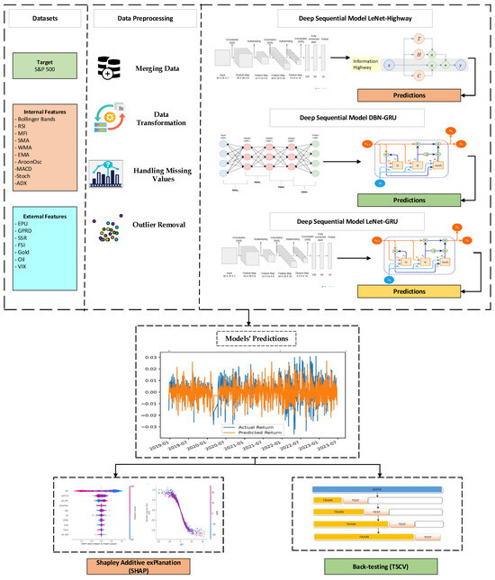
Figure 1. Data-Driven Approach for Forecasting S&P 500 Returns.

3.1. Dataset

The dataset includes S&P 500 stock index as the target variable and a set of internal and external factors as features. The internal factors include values of ten TIs—Bollinger Bands (Boll_ub and Boll_lb), Relative Strength Index (RSI), Aroon Oscillator (AroonOsc), stochastic oscillator (stoch), Average Directional Index (ADX), Money Flow Index (MFI), Moving Average Convergence Divergence (MACD), Simple Moving Average (SMA), Weighted Moving Average (WMA), and Exponential Moving Average (EMA)—calculated from the open, high, low and close prices and volume data of S&P 500 index. Besides, the set of external factors comprises macroeconomic indicators including GPRD, FSI, US EPU, US SSR, gold and oil prices, and VIX. Here, the EPU and SSR are country-specific, and FSI and GPRD are global factors. While VIX is a volatility index measuring the implied volatility of S&P 500 index and is often referred to as the fear index (Sarwar, 2012). The expected volatility of the US stock market in the near future is based on this index. The purpose of selecting these features is to study the influence of both external and internal dynamics on the US stock market in terms of its prediction. Hence, the predictive ability of technical and macroeconomic indicators has been analyzed. The data for all features is of daily frequency for a period of 22.5 years ranging from 1 January 2001 to 26 June 2023. It is a long time period inhibiting the effect of major global events like 9/11 in 2001, GFC 2008, and the COVID-19 pandemic in 2020. The dataset spanning over two decades provides ample data points for training DL models, ensuring the models can capture both short-term and long-term dependencies. Moreover, the start of 2001 marks the period where consistent, high-quality daily data for the selected features became widely available.

Algorithm 1 Algorithm of the Data-Driven Approach Forecasting S&P 500 Returns.

1: Data Collection and Preprocessing:  2: Download S&P 500 index data using YahooFinance API in Python  3: Download data of macroeconomic indicators from their respective sources  4: Calculation of TIs using TA library  5: Merging datasets of external macroeconomic indicators with S&P 500 and TIs  6: Calculate returns taking percentage changes of all variables  7: Remove missing values  8: Remove outliers with 3$\sigma$ rule  9: Data Splitting: 10: Input variables →$X_{\mathrm{train}}$, $X_{\mathrm{test}}$ 11: Target variable →$y_{\mathrm{train}}$, $y_{\mathrm{test}}$ 12: Input: 13: Sequence of input data $X=\{x_1,x_2,...,x_T\}$ 14: Corresponding target outputs $y=\{y_1,y_2,...,y_T\}$ 15: Hyperparameters of the Proposed Models 16: Implementation of the Proposed DL Models: 17: Initialize the parameters (weights and bias vectors) of the proposed model 18: Fit the model ←$X_{train}$, $y_{train}$ 19: Predict stock returns with the trained model ←$X_{test}$ 20: return predictions ${\widehat{y}}_t$ 21: Calculate Evaluation Metrics: 22: RMSE, MAE, MAPE 23: Compare the prediction performance of the proposed models 24: Backtesting: 25: Apply time series cross validation 26: Interpretability of the model: 27: Apply SHAP algorithm

3.2. Data Preprocessing

The daily data of all variables have been accessed from four sources. The S&P 500 index values are extracted using the Python Yahoo Finance API. While the EPU and GPR data have been obtained from a common source1 and the data for SSR2 and FSI3 have been accessed from their respective sources. The data for S&P 500 stock index, Gold, Oil, VIX, and FSI is available for working days only, whereas the data for US EPU, US SSR, and GPRD is inclusive of holidays (including weekends). Therefore, these features have been merged with respect to the dates of S&P 500 index using the Pandas Dataframe.merge function in Python. Please refer to Figure 2 for the merged data.

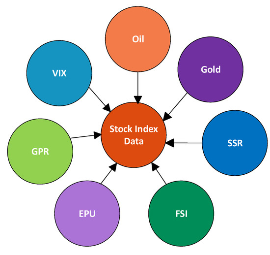
Figure 2. Merging Data.

We have considered the returns (percentage changes) of all variables and removed the outliers (values beyond $\pm 3$ standard deviations) of the resultant dataset using the three sigma rule. The scale of the data has been reduced by taking returns and removing outliers. The final dataset has 4850 samples after deleting those with the missing values. The descriptive statistics of the returns are given in Table 2.

Table 2. Descriptive Statistics of Returns.

	Mean	Std	Min	Max	Skew	Kurt	Range
S&P 500 Return	0.0337	0.9021	−3.6285	3.6499	−0.1889	1.3584	7.2784
GPRD	5.1522	38.1454	−80.5363	167.868	1.0139	1.5556	248.405
US SSR	−0.0596	10.6378	−148.911	144.17	−0.7519	75.3694	293.081
US EPU	10.7329	58.3753	−95.7076	272.3	1.3817	2.4596	368.008
FSI	−1.7076	62.7624	−1121.78	1093.75	−3.9145	135.052	2215.53
Gold	0.0552	0.9388	−3.262	3.3326	−0.1487	0.8682	6.5946
Oil	0.0721	2.2264	−12.2478	14.6764	−0.017	3.3951	26.9242
VIX	−0.0455	5.9211	−21.3836	22.4806	0.4294	1.0353	43.8643
Boll_ub	0.0415	0.2634	−0.9978	0.9773	−0.4255	1.7946	1.9751
Boll_lb	0.0486	0.3205	−1.2966	1.3361	−0.1012	2.6408	2.6327
RSI	0.4435	11.7848	−35.0696	46.1167	0.4028	1.0524	81.1864
Stoch	83.8473	706.68	−100	16978.2	15.9393	300.354	17078.2
ADX	0.3862	15.7659	−28.5681	53.9779	0.3562	0.0578	82.5459
SMA	0.0518	0.279	−1.6113	1.4671	−0.3772	1.891	3.0784
WMA	0.053	0.3105	−1.2611	1.2884	−0.4694	1.1434	2.5494
EMA	0.0506	0.2727	−0.9966	0.9451	−0.5971	0.9829	1.9417
AroonOsc	−8.6186	55.9545	−275	250	−1.7865	7.294	525
MFI	0.7898	15.4275	−51.0437	53.9094	0.3677	0.4529	104.953
MACD	−2.3159	192.607	−3885.21	5973.72	2.144	297.799	9858.92

3.3. Convolutional and Recurrent Neural Networks Applied in the Study

We consider two convolutional neural networks—LeNet and DBN—and two recurrent neural networks—GRU and Highway—to propose our hybrid DL models for forecasting S&P 500 returns. Moreover, these are the benchmark models to compare the performance of our proposed models in this study. A brief introduction of these single models and the details of their proposed combinations are given in the following subsections.

3.3.1. Gated Recurrent Unit (GRU)

A gated recurrent unit, being a simplification of LSTM, is a special type of RNN introduced by Chung et al. (2014). It has been developed to reduce the computational complexity of LSTM to process sequential data like speech, text, and time series. GRU has two gates—the reset gate and the update gate—in contrast to the three gates of LSTM (forget, input, and output gates). The reset gate of GRU has the same function as the forget gate in LSTM, which is to determine the chunk of information coming from the hidden state to be forgotten, whereas the update gate updates the hidden state with the selective input information. This way, there is control over the flow of information passing through a GRU unit. The underlying purpose is to update the hidden state and calculate the output at every time step. The structure of a GRU cell is shown in Figure 3 (Su & Kuo, 2019).

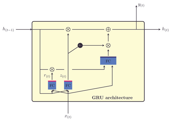
Figure 3. Architecture of a GRU Cell.

Assume that $x_t$ is the input at a given time step t, $h_{t-1}$ is the hidden state at the previous time step $t-1$, $W_z$ and $b_z$ are the weights and biases for the update gate and $W_r$ and $b_r$ are the weights and biases for the reset gate, the respective outputs of the update and reset gates as $z_t$ and $r_t$ take the form as:

$$\begin{array}{c}\hfill z_t=\sigma (W_z·[h_{t-1},x_t]+b_z)\end{array}$$

(2)

$$\begin{array}{c}\hfill r_t=\sigma (W_r·[h_{t-1},x_t]+b_r)\end{array}$$

(3)

Moreover, the candidate hidden state ${\tilde{h}}_t$ of the GRU cell with $W_h$ and $b_h$ as its weights and biases is updated as:

$$\begin{array}{c}\hfill {\tilde{h}}_t=\tan \mathrm{h}(W_h·[r_t\odot h_{t-1},x_t]+b_h)\end{array}$$

(4)

With ⊙ as the hadamard product, the final output of the GRU cell is the updated hidden state $h_t$ calculated as:

$$\begin{array}{c}\hfill h_t=(1-z_t)\odot h_{t-1}+z_t\odot {\tilde{h}}_t\end{array}$$

(5)

3.3.2. Recurrent Highway Networks (RHNs)

A highway network is a deep feed-forward NN having hundreds of layers with skip connections that regulate the flow of information. These networks have been designed and introduced by Srivastava et al. (2015) with the main purpose of resolving the issues of gradient-based training of very deep networks. These are inspired by the LSTM architecture. The depth of NNs is crucial for solving complex research problems and large datasets. However, this depth poses challenges to the training of such networks (Sonkavde et al., 2023). The highway networks have been introduced as a solution to this problem. They enable gradient-based training of hundreds of layers using multiple activation functions. The equations for the basic unit of a highway network are:

$$\begin{array}{c}\hfill T\left(x\right)=\sigma (W_T·x+b_T)\end{array}$$

(6)

$$\begin{array}{c}\hfill C\left(x\right)=1-T\left(x\right)\end{array}$$

(7)

$$\begin{array}{c}\hfill H\left(x\right)=\mathrm{ReLU}(W_H·x+b_H)\end{array}$$

(8)

$$\begin{array}{c}\hfill Y\left(x\right)=T\left(x\right)·H\left(x\right)+C\left(x\right)·x\end{array}$$

(9)

Here x is the input to the network; $T\left(x\right)$ is the transform gate and $C\left(x\right)$ is the carry gate; $H\left(x\right)$ is the transformed output; $W_T$ and $b_T$ are the weights and bias terms for the transformation gate; $W_H$ and $b_H$ are the weights and bias terms for the transformation; $sigma$ is the sigmoid activation function and $ReLU$ is the rectified linear unit activation function; and lastly, $Y\left(x\right)$ is the final output.

We are predicting stock returns by incorporating the linear activation function in the final output layer of the highway network. The basic architecture of a highway network is shown in Figure 4, (Tao et al., 2018).

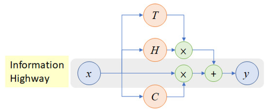
Figure 4. Architecture of Recurrent Highway Network.

3.3.3. LeNet

LeNet is one of the initial CNNs proposed by LeCun et al. (1998). It has been primarily designed for recognition of images of handwritten digits and laid the foundation for further advancements in deep learning. The basic structure of LeNet, as shown in Figure 5, comprises seven layers, including two 5 × 5 convolutional layers, 2 average pooling layers and three dense layers with non-linear activation functions (Wang et al., 2017). LeNet bascially refers to LeNet-5, which is the fifth iteration of the LeNet CNN model. It has unique convolutional filters or kernels that identify the inherent patterns of the data. It has been widely used for object recognition and natural language processing. Moreover, it has been used to predict the direction of S&P 500 using data of per minute frequency (Sim et al., 2019). The empirical results show that CNNs can better predict S&P 500 than ANN and SVM. In another work, an optimized CNN has been used by Chung and Shin (2020) to predict the Korean stock index KOSPI movement using TIs as features. The optimized CNN outperformed simple CNN and ANN in terms of prediction performance.

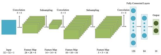
Figure 5. Architecture of LeNet.

3.3.4. Deep Belief Networks (DBNs)

A deep belief network is an unsupervised learning algorithm comprising of two different NNs—Restricted Boltzman Machines (RBMs) and belief networks. RBMs are similar to the regular Boltzman machines, with the exception that they are not fully connected and therefore they are named as ’restricted’. The RBMs are used for pre-training and the back propagation NN is employed for reverse fine-tuning in a DBN.

DBN involves multiple layers with conditional dependencies; therefore, it has an extensive set of equations. However, a simplified set of equations for its building block are represented here (Zhang & Ci, 2020). There are $N_h$ nodes in the hidden layers and $N_v$ nodes in the visible layer. Assume the binary states of the visible node i and hidden node j as $v_i$ and $h_j$, the weight between them as $w_{i}j$ and the biases as $a_i$ and $b_j$. The equations for RBM layers will be:

The visible layer consists of observable variables:

$$\begin{array}{c}\hfill P(v_i=1)=\sigma \left(\sum _{j=1}^{N_h}{W}_{ij}{h}_j+b_i\right)\end{array}$$

(10)

The hidden layer consists of latent variables:

$$\begin{array}{c}\hfill P(h_j=1)=\sigma \left(\sum _{i=1}^{N_v}{W}_{ij}{v}_i+c_j\right)\end{array}$$

(11)

The joint energy of the RBM is given by:

$$\begin{array}{c}\hfill E(v,h)=-\sum _{i=1}^{N_v}\sum _{j=1}^{N_h}{W}_{ij}{v}_i{h}_j-\sum _{i=1}^{N_v}{b}_i{v}_i-\sum _{j=1}^{N_h}{c}_j{h}_j\end{array}$$

(12)

The conditional probabilities are given by the sigmoid function:

$$\begin{array}{c}\hfill P(h_j=1|v)=\sigma \left(\sum _{i=1}^{N_v}{W}_{ij}{v}_i+c_j\right)\end{array}$$

(13)

A DBN is composed of multiple RBMs stacked on top of each other. The hidden layer of one RBM becomes the visible layer of the next RBM, such that:

$$\begin{array}{c}\hfill P(v_i^{\left(k\right)}=1|h^{\left(k\right)})=\sigma \left(\sum _{j=1}^{N^{(k-1)}}{W}_{ij}^{\left(k\right)}{h}_j^{(k-1)}+b_i^{\left(k\right)}\right)\end{array}$$

(14)

$$\begin{array}{c}\hfill P(h_j^{\left(k\right)}=1|v^{\left(k\right)})=\sigma \left(\sum _{i=1}^{N^{\left(k\right)}}{W}_{ij}^{\left(k\right)}{v}_i^{\left(k\right)}+c_j^{\left(k\right)}\right)\end{array}$$

(15)

However, the output layer of a DBN for regression can be modified as:

$$\begin{array}{c}\hfill {\widehat{y}}_i=\sum _{j=1}^{N^{\left(k\right)}}{W}_{ij}^{\left(k\right)}{h}_j^{(k-1)}+b_i^{\left(k\right)}\end{array}$$

(16)

Here ${\widehat{y}}_i$ is the predicted stock return for the $ith$ sample, and $h_j^{(k-1)}$ is the activation from the hidden layer of the previous RBM. The linear activation function will be used instead of the sigma function. The framework of the DBN regression model is depicted in Figure 6 (Boesch, 2024).

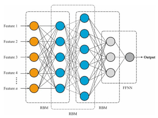
Figure 6. Architecture of DBN.

3.4. Proposed Hybrid Deep Learning Models

In our data-driven approach, the hybrid DL models are combined on the idea of an encoder-decoder framework. The encoder is first applied to filter the original inputs for feature extraction, and then the decoder makes predictions using the extracted features as input. The hybrid NNs have been extensively worked upon for stock market prediction (Jia et al., 2023; Sonkavde et al., 2023). This study also employs hybrid NNs for predicting stock returns of S&P 500. Specifically, we employ a CNN variant to extract features and then a recurrent architecture for predictions. Though RNNs are more acknowledged for doing well with the sequential data, CNNs can also be applied successfully for sequential modeling (Jerez & Kristjanpoller, 2020). They also have the advantages of avoiding gradient and memory problems. In some studies, CNNs outperform LSTMs (Bai et al., 2018). Hence, convolutional neural networks LeNet and DBN are used for features’ extraction at the first tier, and recurrent neural networks GRU and Highway are used for prediction at the second tier. The proposed three hybrid sequential models are DBN-GRU, LeNet-GRU, and LeNet-Highway. The topologies of the proposed DBN-GRU, LeNet-GRU, and LeNet-Highway models are given in Table 3, Table 4 and Table 5.

Table 3. Topology of the Proposed Model 1: DBN-GRU.

Models	Topology
DBN	Input (X)
	Hidden Layer 1 (Units = 128)
	Hidden Layer 2 (Units = 64)
	Hidden Layer 3 (Units = 32)
	Flatten Layer ()
GRU	Input (Flatten layer output of DBN)
	GRU (Units = 32, Activation = tanh)
	Dense Layer (Units = 1, Activation = linear)

Table 4. Topology of the Proposed Model 2: LeNet-GRU.

Models	Topology
LeNet	Input (X)
	Conv 1D Layer (Units = 6, kernel_size = 3, padding = same, Activation = tanh)
	Average Pooling (pool_size = 2, padding = same)
	Conv 1D Layer (Units = 64, kernel_size = 3, padding = same, Activation = tanh)
	Average Pooling (pool_size = 2, padding = same)
	Flatten Layer ()
	Dense Layer (Units = 32, Activation = tanh)
	Dense layer (Units = 16, Activation = tanh)
GRU	Input (Dense layer output of LeNet)
	GRU(Units = 32, Activation = tanh)
	Dense Layer(Units = 1, Activation = linear)

Table 5. Topology of the Proposed Model 3: LeNet-Highway.

Models	Topology
LeNet	Input (X)
	Conv 1D Layer (Units = 6, kernel_size = 3, padding = same, Activation = tanh)
	Average Pooling (pool_size = 2, padding = same)
	Conv 1D Layer (Units = 64, kernel_size = 3, padding = same, Activation = tanh)
	Average Pooling (pool_size = 2, padding = same)
	Flatten Layer ()
	Dense Layer (Units = 32, Activation = tanh)
	Dense layer (Units = 16, Activation = tanh)
Highway	Input (Dense Layer output of LeNet)
	Transform Gate with Activation = sigmoid
	Carry Gate
	Transformation with Activation = sigmoid
	Highway Output is the combination of outputs of transform gate and carry gate
	Hidden Layer1 (Units = 64, Activation = tanh)
	Hidden Layer2 (Units = 64, Activation = tanh)
	Hidden Layer3 Dense (Units = 32, Activation = tanh)
	Hidden Layer4 Dense (Units = 32, Activation = tanh)
	Output (Units = 1 and Activation = linear)

The choice of DL models to forecast S&P 500 returns is justified by their ability to capture complex, non-linear relationships of the uncertainty factors US EPU, FSI, GPR, and SSR with stock returns and volatility. Literature highlights that these risk factors often lack linear relationships with market dynamics, making non-linear models like DL more suitable for forecasting (Aye et al., 2018; Balcilar et al., 2019). Besides, hybrid models are known to leverage the strengths of different neural network architectures, enabling enhanced predictive performance for complex financial time series data. Existing literature underscores that hybrid architectures outperform standalone DL models by addressing their limitations, such as overfitting and weak generalization in dynamic systems (Hajirahimi & Khashei, 2019; Pradeepkumar & Ravi, 2018).

4. Results and Discussion

The accuracy of the applied prediction models has been gauged using three evaluation metrics: RMSE, MAE, and MAPE. Among these, RMSE and MAE are scale-dependent. These can be used for comparing different models on the same data, as is the case in this study. Besides, MAPE is independent of the scale of the data and is a percentage measure of the model’s accuracy (Mahajan et al., 2022). However, it needs a meaningful zero and can be undefined for the actual values closer to zero. Our study evaluates the prediction performance of the benchmark and the proposed models by calculating both scale-dependent RMSE and MAE and scale-independent MAPE.

The evaluation metrics of our applied models are reported in Table 6. This table presents deep models in order of descending RMSE. It is evident that the three proposed models, DBN-GRU, LeNet-GRU and LeNet-Highway, outperform their component models (DBN, GRU, LeNet and Highway) for the three evaluation metrics. Hence, the prediction performance of the proposed hybrid models is better than the single deep models. The result aligns with the previous studies that suggest that combined models are more viable for time series modeling and can enhance the forecasting accuracy in contrast to single models used separately (Hajirahimi & Khashei, 2019; Liang et al., 2019; Pradeepkumar & Ravi, 2018).

Table 6. Evaluation of Prediction Performance.

Model	Performance Metrics
	RMSE	MAE	MAPE
DBN	0.0076	0.0046	2.29%
GRU	0.0075	0.0059	3.01%
Highway	0.0067	0.0037	1.48%
LeNet	0.0049	0.0038	1.24%
DBN, GRU Hybrid	0.0045	0.0031	1.26%
LeNet, GRU Hybrid	0.0045	0.0031	1.07%
LeNet, Highway Hybrid	0.0040	0.0028	0.97%

To further verify the prediction performance of the proposed hybrid models, the forecasted returns of the S&P 500 were plotted against the actual returns for the out-of-sample values in Figure 7, Figure 8 and Figure 9. These plots show that the proposed models have a better predictive ability for forecasting S&P returns over the testing period. Moreover, these plots present varying but reasonable degrees of randomness in their forecasts. Similar results were also plotted for the prediction performance of the single benchmark models.

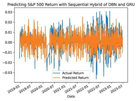
Figure 7. S&P500 Return Prediction with Hybrid DBN-GRU Model.

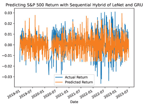
Figure 8. S&P500 Return Prediction with Hybrid LeNet-GRU Model.

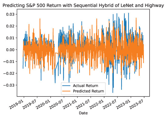
Figure 9. S&P500 Return Prediction with Hybrid LeNet-Highway Model.

Notably, the hybrid LeNet–Highway model outperforms all other models with the lowest RMSE, MAE and MAPE values, as shown in Figure 10, Figure 11 and Figure 12, respectively. Additionally, the prediction performance of DBN–GRU and LeNet–GRU is almost similar. This result can be due to using the GRU for final predictions in both models. It also suggests that DBN and LeNet perform equally well for feature extraction. However, LeNet is the best-performing solo model among DBN, GRU, and Highway. A CNN variant outperforming sequential RNNs is supported in the literature (Bai et al., 2018; Jerez & Kristjanpoller, 2020).

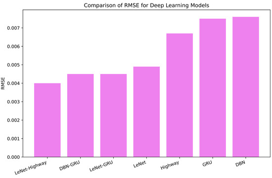
Figure 10. RMSE of the Applied Deep Models.

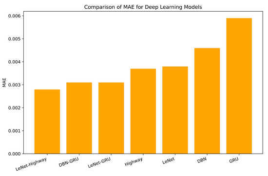
Figure 11. MAE of the Applied Deep Models.

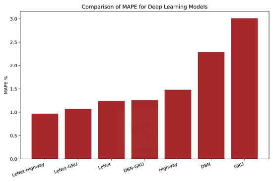
Figure 12. MAPE of the Applied Deep Models.

When we compare the prediction performance of the proposed hybrid models with that of their component models, we find that the DBN-GRU hybrid has approximately 41%, 33%, and 45% lower RMSE, MAE, and MAPE values respectively, than those of DBN, which is performing better than GRU. This can be verified by examining the bar chart comparing errors in Figure 13. Similarly, LeNet performs better than GRU for all metrics. Their hybrid LeNet-GRU outperforms LeNet with around 8%, 18%, and 14% lower RMSE, MAE, and MAPE, respectively, as shown in Figure 14. Lastly, our best-performing LeNet-Highway hybrid model beats LeNet with lower RMSE, MAE, and MAPE of around 11%, 10%, and 23% respectively, as shown in Figure 15.

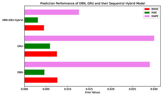
Figure 13. Comparison of Error Values of DBN, GRU and their Hybrid Model.

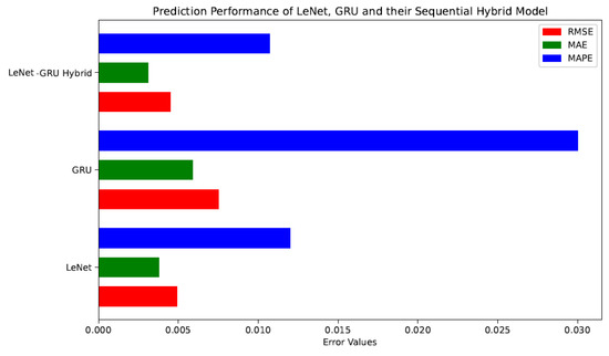
Figure 14. Comparison of Error Values of LeNet, GRU and their Hybrid Model.

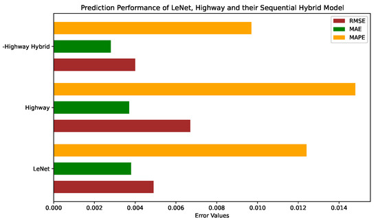
Figure 15. Comparison of Error Values of LeNet, Highway Network and their Hybrid Model.

While our results demonstrate the superior forecasting performance of the proposed hybrid DL models, we acknowledge that combining different architectures may lead to higher computational costs, potentially limiting their real-time application. This challenge can be addressed by leveraging techniques such as model optimization and parallel processing to reduce computational overhead without significantly compromising performance. However, there must be a trade-off between the model’s complexity and forecasting performance. Given these considerations, the primary focus of this study is to enhance forecasting accuracy, ensuring that the models effectively capture the complex, non-linear dynamics of financial markets.

5. Time Series Cross Validation

Cross validation is a method to assess the generalizability of a model’s learning to a new dataset. For prediction models, it is applied to estimate that how accurately the forecasting model is going to predict in real time (Donate et al., 2013). Time Series Cross Validation (TSCV) is used in ML to assess the generalizability of a prediction model for new or unseen data. It is different from the k-fold cross validation in terms of data splitting. The k-fold method is not suitable for time series validation as it randomly splits the data into testing and training sets without maintaining order of the training and testing subsets (Zhou, 2021). However, the order of data samples matters for sequential data as is the case for stock data. Test samples must be preceded by consecutive training samples and this order is to be maintained for all folds of the validation technique. The prediction model is trained on the training samples and tested on the validation samples and the process is repeated for a given number of folds and sizes of the validation data. This way, the predictive performance of the model is assessed across time.

In this study, we have used TSCV for analyzing the predictive ability of our best prediction model, LeNet-Highway. The model has been cross validated by comparing the results in terms of RMSE, MAE, and MAPE for different mixes of number of folds (k = 10, 20) and size of validation data (100, 10, 1) (Zhou, 2021). We get the results of cross validation comparable with the prediction performance of the LeNet-Highway and its component models, LeNet and Highway, for 10 folds and 100 validation samples. The results of this combination are presented in Table 7 and its results confirm the generalizability of our proposed model LeNet-Highway. The cross validation of our proposed model also postulates that future returns can be predicted based on their previous values. Historical data of the stock market provides patterns for the predictability of future performance of the market as established by many studies in the existing literature (Gajamannage et al., 2023; Gupta et al., 2022; Huang et al., 2023; Ma & Yan, 2022; Rezaei et al., 2021). However, this is in contradiction to the hypotheses of efficient markets (Fama, 1970) and random walk (Godfrey et al., 1964).

Table 7. Results of Time Series Cross Validation for k = 10 and validation_samples = 100.

Models	RMSE	MAE	MAPE
LeNet	0.0049	0.0038	1.24%
Highway	0.0067	0.0037	1.48%
LeNet-Highway	0.004	0.0028	0.97%
TSCV for 10 folds	0.0039 0.0051 0.0064 0.0099 0.0032 0.0021 0.0037 0.0049 0.0053 0.0026	0.0027 0.0044 0.0059 0.0090 0.0023 0.0014 0.0028 0.0036 0.0041 0.0021	1.35% 3.77% 4.83% 2.58% 0.71% 0.33% 0.76% 0.52% 0.59% 3.00%
Average across all folds	0.0047	0.0038	1.84%

6. SHapley Additive exPlanation (SHAP) for Explaining the Model’s Predictions

DL models are also referred to as ’black-box’ models as they cannot explain how they produce certain forecasts. Their predictions are not explainable unless they have been verified with some customized tools. Such tools offer interpretability that helps build trust in the model’s predictions. Moreover, it helps in detecting biases, if any, in the data or the model. SHAP is one such tool, based on Shapley values, which use game theory to credit each variable for the predictions of the model.

SHapley Additive exPlanation (SHAP) is an Explainable Artificial Intelligence (XAI) technique for understanding the intricate choices made by deep models. It has been proposed by Lundberg and Lee (2017) that explains individual predictions. By giving each variable an interpretable value and providing information on how each contributes to the model’s predictions individually, SHAP overcomes the opacity that deep models have by design. It provides a thorough and easy to understand analysis of the significance of every input variable for forecasting the target variable. Practitioners and researchers can better understand the significant variables influencing a model’s output with the aid of this factor-wise attribution.

In this research, we have implemented SHAP to explain the forecasts of our best prediction model LeNet-Highway. First, a background summary is produced by applying K-means clustering to the training dataset. We use 25 clusters of our data samples using K-means. The model’s predictions and a background summary derived from k-mean clustering are used in the design of a SHAP explainer known as ‘Kernel Explainer’, which measures the SHAP values for each variable. These values provide information about the role that variable plays in the model’s ability to predict outcomes based on a particular sample. We generate a force plot and a summary plot using these shap values to know the contribution of variables in the model’s predictions. For a variable and a sample, each point on the summary plot represents a shapley value. The feature determines the position on the y-axis, while the shapley value determines the position on the x-axis. The variable’s value is represented by color, ranging from low to high. In the summary plot, the y-axis direction of the jittered overlapped points helps us understand the distribution of the Shapley values for each variable. The variables are listed in descending order of significance.

As shown in Figure 16, the summary plot orders variables based on their importance in predicting the S&P 500 return. This plot summarizes the top ten important variables for predicting the S&P 500 using our proposed LeNet-Highway hybrid model. The most significant variables of our dataset include seven macroeconomic indicators and three TIs. It shows that VIX is our prediction model’s most important input variable. Indeed, the higher percentage change values in VIX result in lower stock return values. Thus, a significant negative relationship exists between VIX and S&P 500 returns (Campisi et al., 2023; Sarwar, 2012). This finding aligns with previous studies, such as Adeloye et al. (2024); Campisi et al. (2023); Sarwar (2012), which suggest that stock market volatility and market performance are negatively associated, and increased volatility significantly diminishes market outcomes in the long run. The change in volatility is followed by the contemporary factors of FSI and US EPU, the second and third most important predictors of S&P 500 returns. This is well-supported by the literature, which establishes the significant predictive power of contemporaneous uncertainty factors like EPU for market returns and volatility (Aye et al., 2018; Brogaard & Detzel, 2015). Interestingly, EPU, as a risk factor, has been shown to predict future returns in financial markets and may be compensated with a risk premium (Pastor & Veronesi, 2013; Phan et al., 2018). It is important to note that the four contemporary macroeconomic indicators—percentage changes in US EPU, FSI, GPRD and US SSR—are important variables for predicting the S&P 500 return. Similarly, the global FSI has been identified as the most significant predictor in equity markets by Liang et al. (2023), while contractionary monetary policy, as reflected in SSR, has been found to decrease stock returns (Tokmakcioglu & Ozcelebi, 2020). However, there are also some contradictions, and the impact of uncertainty factors such as EPU is not significant for some equity markets (Li et al., 2016; Mensi et al., 2014). In addition, the direction and strength of the association between EPU and stock markets appear to depend on market conditions, like credit constraints (Carrière-Swallow & Céspedes, 2013). These mixed findings underline the complex and heterogeneous role of contemporary uncertainty factors in predicting stock market returns across different regions and economic conditions. Besides, oil and gold returns are also included in the list of important explanatory variables. Moreover, the summary plot shows that aroonOsc, ADX, and MACD returns are significant TIs for US market forecasts. We find support for many studies that establish the importance of these indicators in capturing market trends and momentum (Kamara et al., 2022; Ma & Yan, 2022; Stein, 2022).

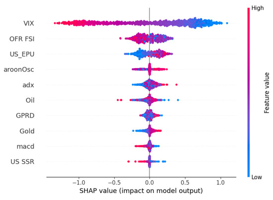
Figure 16. SHAP Summary Plot for LeNet-Highway.

In addition, a force plot visually shows how each variable in a model influences an individual forecast. It highlights the contribution of each variable, pushing the prediction higher (positive value) or lower (negative value) relative to the baseline prediction. At the point where the data sample is actually predicted, these forces balance each other. In the force plot shown in Figure 17, the baseline value is set to be 0.35, and the most important variable is VIX that is in line with the results of the summary plot. Higher values of variables (in red) force the predicted return to lower side while the lower values of variables (in blue) force it to the higher side. For instance, higher values of change in VIX lower the expected return, and lower values of change in oil increase the expected return (Aye et al., 2018; Brogaard & Detzel, 2015). It is important to note that these values are given for a specific sample.

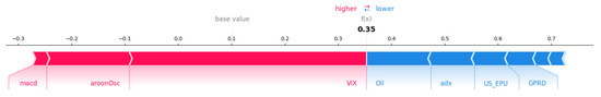
Figure 17. Force Plot for LeNet-Highway.

7. Conclusions and Future Work

In this study, we adopted a data-driven approach to forecast the stock market by integrating several macroeconomic and TIs as predictors. We combined convolutional and recurrent neural networks to develop three novel deep hybrid models: DBN-GRU, LeNet-GRU, and LeNet-Highway. Using CNN variants (LeNet and DBN) for feature extraction and recurrent NNs (GRU and Highway) for prediction, we sequentially combined these deep models to examine the predictive power of macroeconomic and technical indicators for the US stock market. Our findings reveal that the US stock market is indeed predictable, with the LeNet-Highway hybrid model emerging as the most accurate prediction model of S&P 500 returns, delivering the lowest RMSE, MAE, and MAPE values among all models tested. This model outperforms the second-best LeNet model by 11%, 10%, and 23% in RMSE, MAE, and MAPE, respectively.

Significantly, our analysis indicates that both LeNet and DBN are effective at extracting relevant features, confirming the superior feature extraction capability of CNNs in this context. Importantly, all three hybrid models demonstrated lower prediction errors than their component models, underscoring the enhanced predictive power of combining CNNs with recurrent networks. This synergy leverages the feature extraction strength of CNNs alongside the sequential pattern-capturing ability of RNNs, leading to improved forecasts of S&P 500 returns. Furthermore, SHAP values provided insight into the model’s interpretability, identifying VIX, FSI, and US EPU as the most influential factors in predicting S&P 500 returns.

These findings emphasize the predictive importance of macroeconomic indicators over TIs in forecasting stock returns. The robustness of our best-performing model was confirmed through time series cross-validation, affirming its generalizability on unseen datasets. This study highlights the critical role of advanced DL frameworks in enhancing stock market prediction accuracy. Accurate market predictions are crucial for stock market stakeholders, as they enable more informed investment decisions, effective risk management, and strategic asset allocation. Enhanced predictive accuracy provides financial analysts, portfolio managers, and institutional investors with insights that can optimize returns, anticipate market shifts, and maintain a competitive edge in the dynamic financial landscape.

Our study has several limitations that present opportunities for future research. While this study focuses on the US stock market, it can be extended to other countries’ markets to enable cross-market comparisons. However, data for country-specific EPUs is often available only at a monthly frequency, which may impact prediction granularity. Future studies could also incorporate additional factors, such as foreign exchange rates, cryptocurrency prices, and other relevant variables, to assess their influence on stock market prediction accuracy. Moreover, indicators like the Twitter-based Economic Uncertainty (TEU) could be examined for their predictive potential. Besides, testing alternative DL models beyond GRU, Highway Networks, DBN, and LeNet may offer further insights into the stock market’s data learning capabilities and predictive performance. However, it should be pointed out that the proposed hybrid models do not address Unobserved Heterogeneity (UH), which refers to variations in data caused by unobserved factors. These unmeasured factors may impact the accuracy and reliability of predictions (Hamed et al., 2022). Thus, future research could explore methods like latent variable models or hybrid approaches combining statistical techniques with DL to better account for UH.

References

- Adeloye, F. C., Olawoyin, O., & Chinaemerem, D. (2024). Economic policy uncertainty and financial markets in the united state. International Journal of Research and Innovation in Social Science, 8(6), 998–1016. [Google Scholar] [CrossRef]
- Alqahtani, A., & Martinez, M. (2020). Us economic policy uncertainty and gcc stock market. Asia-Pacific Financial Markets, 27(3), 415–425. [Google Scholar] [CrossRef]
- Andrei, D., & Hasler, M. (2015). Investor attention and stock market volatility. The Review of Financial Studies, 28(1), 33–72. [Google Scholar] [CrossRef]
- Antonakakis, N., Chatziantoniou, I., & Filis, G. (2017). Oil shocks and stock markets: Dynamic connectedness under the prism of recent geopolitical and economic unrest. International Review of Financial Analysis, 50, 1–26. [Google Scholar] [CrossRef]
- Arouri, M., Estay, C., Rault, C., & Roubaud, D. (2016). Economic policy uncertainty and stock markets: Long-run evidence from the us. Finance Research Letters, 18, 136–141. [Google Scholar] [CrossRef]
- Aslam, F., Mohti, W., Ali, H., & Ferreira, P. (2023). Interplay of multifractal dynamics between shadow policy rates and stock markets. Heliyon, 9, e18114. [Google Scholar] [CrossRef] [PubMed]
- Aye, G. C., Balcilar, M., Demirer, R., & Gupta, R. (2018). Firm-level political risk and asymmetric volatility. The Journal of Economic Asymmetries, 18, e00110. [Google Scholar] [CrossRef]
- Baek, Y., & Kim, H. Y. (2018). Modaugnet: A new forecasting framework for stock market index value with an overfitting prevention lstm module and a prediction lstm module. Expert Systems with Applications, 113, 457–480. [Google Scholar] [CrossRef]
- Bai, S., Kolter, J. Z., & Koltun, V. (2018). An empirical evaluation of generic convolutional and recurrent networks for sequence modeling. arXiv, arXiv:1803.01271. [Google Scholar]
- Baker, S. R., Bloom, N., & Davis, S. J. (2016). Measuring economic policy uncertainty. The Quarterly Journal of Economics, 131(4), 1593–1636. [Google Scholar] [CrossRef]
- Balcilar, M., Gupta, R., Kim, W. Y., & Kyei, C. (2019). The role of economic policy uncertainties in predicting stock returns and their volatility for hong kong, malaysia and south korea. International Review of Economics & Finance, 59, 150–163. [Google Scholar]
- Bali, T. G., Brown, S. J., & Tang, Y. (2022). Disagreement in economic forecasts and equity returns: Risk or mispricing? China Finance Review International. ahead-of-print. [Google Scholar]
- Black, F. (1995). Interest rates as options. The Journal of Finance, 50(5), 1371–1376. [Google Scholar] [CrossRef]
- Boesch, G. (2024, February 8). Deep belief networks: A comprehensive overview. Available online: https://viso.ai/deep-learning/deep-belief-networks/ (accessed on 28 October 2024).
- Bouras, C., Christou, C., Gupta, R., & Suleman, T. (2019). Geopolitical risks, returns, and volatility in emerging stock markets: Evidence from a panel garch model. Emerging Markets Finance and Trade, 55(8), 1841–1856. [Google Scholar] [CrossRef]
- Brogaard, J., & Detzel, A. (2015). The asset-pricing implications of government economic policy uncertainty. Management Science, 61(1), 3–18. [Google Scholar] [CrossRef]
- Caldara, D., & Iacoviello, M. (2017). Measuring geopolitical risk. Technical report. Board of Governors of the Federal Reserve System. [Google Scholar]
- Caldara, D., & Iacoviello, M. (2022). Measuring geopolitical risk. American Economic Review, 112(4), 1194–1225. [Google Scholar] [CrossRef]
- Campisi, G., Muzzioli, S., & Baets, B. D. (2023). A comparison of machine learning methods for predicting the direction of the us stock market on the basis of volatility indices. International Journal of Forecasting, 40, 869–880. [Google Scholar] [CrossRef]
- Carrière-Swallow, Y., & Céspedes, L. F. (2013). The impact of uncertainty shocks in emerging economies. Journal of International Economics, 90(2), 316–325. [Google Scholar] [CrossRef]
- Celebi, K., & Hönig, M. (2019). The impact of macroeconomic factors on the german stock market: Evidence for the crisis, pre-and post-crisis periods. International Journal of Financial Studies, 7(2), 18. [Google Scholar] [CrossRef]
- Chalmers, J., Picard, N., & Eastman, H. (2023, January 18). Pwc’s global investor survey 2022, Harvard Law School Forum on Corporate Governance.
- Chiang, T. C. (2019). Economic policy uncertainty, risk and stock returns: Evidence from g7 stock markets. Finance Research Letters, 29, 41–49. [Google Scholar] [CrossRef]
- Christou, C., Cunado, J., Gupta, R., & Hassapis, C. (2017). Economic policy uncertainty and stock market returns in pacific rim countries: Evidence based on a bayesian panel var model. Journal of Multinational Financial Management, 40, 92–102. [Google Scholar] [CrossRef]
- Chung, H., & Shin, K. S. (2020). Genetic algorithm-optimized multi-channel convolutional neural network for stock market prediction. Neural Computing and Applications, 32, 7897–7914. [Google Scholar] [CrossRef]
- Chung, J., Gulcehre, C., Cho, K., & Bengio, Y. (2014). Empirical evaluation of gated recurrent neural networks on sequence modeling. arXiv, arXiv:1412.3555. [Google Scholar]
- Claus, E., Claus, I., & Krippner, L. (2014). Asset markets and monetary policy shocks at the zero lower bound. Reserve Bank of New Zealand. [Google Scholar]
- Claus, E., Claus, I., & Krippner, L. (2018). Asset market responses to conventional and unconventional monetary policy shocks in the united states. Journal of Banking & Finance, 97, 270–282. [Google Scholar]
- Das, D., Kannadhasan, M., & Bhattacharyya, M. (2019). Do the emerging stock markets react to international economic policy uncertainty, geopolitical risk and financial stress alike? The North American Journal of Economics and Finance, 48, 1–19. [Google Scholar] [CrossRef]
- Das, D., Maitra, D., Dutta, A., & Basu, S. (2022). Financial stress and crude oil implied volatility: New evidence from continuous wavelet transformation framework. Energy Economics, 115, 106388. [Google Scholar] [CrossRef]
- Donate, J. P., Cortez, P., Sánchez, G. G., & De Miguel, A. S. (2013). Time series forecasting using a weighted cross-validation evolutionary artificial neural network ensemble. Neurocomputing, 109, 27–32. [Google Scholar] [CrossRef]
- Evans, M. D., & Hnatkovska, V. V. (2014). International capital flows, returns and world financial integration. Journal of International Economics, 92(1), 14–33. [Google Scholar] [CrossRef]
- Fama, E. F. (1970). Efficient capital markets: A review of theory and empirical work. The Journal of Finance, 25(2), 383–417. [Google Scholar] [CrossRef]
- Ftiti, Z., & Hadhri, S. (2019). Can economic policy uncertainty, oil prices, and investor sentiment predict islamic stock returns? A multi-scale perspective. Pacific-Basin Finance Journal, 53, 40–55. [Google Scholar] [CrossRef]
- Gajamannage, K., Park, Y., & Jayathilake, D. I. (2023). Real-time forecasting of time series in financial markets using sequentially trained dual-lstms. Expert Systems with Applications, 223, 119879. [Google Scholar] [CrossRef]
- Gao, R., Zhang, X., Zhang, H., Zhao, Q., & Wang, Y. (2022). Forecasting the overnight return direction of stock market index combining global market indices: A multiple-branch deep learning approach. Expert Systems with Applications, 194, 116506. [Google Scholar] [CrossRef]
- Ghani, M., & Ghani, U. (2023). Economic policy uncertainty and emerging stock market volatility. Asia-Pacific Financial Markets, 1–17. [Google Scholar] [CrossRef]
- Godfrey, M. D., Granger, C. W., & Morgenstern, O. (1964). The random-walk hypothesis of stock market behavior. Kyklos, 17(1), 1–30. [Google Scholar] [CrossRef]
- Gupta, R., Marfatia, H. A., & Olson, E. (2020). Effect of uncertainty on us stock returns and volatility: Evidence from over eighty years of high-frequency data. Applied Economics Letters, 27(16), 1305–1311. [Google Scholar] [CrossRef]
- Gupta, U., Bhattacharjee, V., & Bishnu, P. S. (2022). Stocknet—gru based stock index prediction. Expert Systems with Applications, 207, 117986. [Google Scholar] [CrossRef]
- Hajirahimi, Z., & Khashei, M. (2019). Hybrid structures in time series modeling and forecasting: A review. Engineering Applications of Artificial Intelligence, 86, 83–106. [Google Scholar] [CrossRef]
- Hamed, M. M., Ali, H., & Abdelal, Q. (2022). Forecasting annual electric power consumption using a random parameters model with heterogeneity in means and variances. Energy, 255, 124510. [Google Scholar] [CrossRef]
- Hong, H., Torous, W., & Valkanov, R. (2007). Do industries lead stock markets? Journal of Financial Economics, 83(2), 367–396. [Google Scholar] [CrossRef]
- Hu, Z., Kutan, A. M., & Sun, P. W. (2018). Is us economic policy uncertainty priced in china’s a-shares market? evidence from market, industry, and individual stocks. International Review of Financial Analysis, 57, 207–220. [Google Scholar] [CrossRef]
- Huang, Y., Ma, F., Bouri, E., & Huang, D. (2023). A comprehensive investigation on the predictive power of economic policy uncertainty from non-us countries for us stock market returns. International Review of Financial Analysis, 87, 102656. [Google Scholar] [CrossRef]
- Ilgın, K. (2024). The effect of financial stress on stock markets: An example of mint economies. Marmara Üniversitesi İktisadi ve İdari Bilimler Dergisi, 46(2), 452–467. [Google Scholar] [CrossRef]
- Index, OFR Financial Stress. (2023, December 15). Financial stress index. Available online: https://www.financialresearch.gov/financial-stress-index/ (accessed on 15 December 2023).
- Ivanyuk, V. (2022). Methodology for constructing an experimental investment strategy formed in crisis conditions. Economies, 10(12), 325. [Google Scholar] [CrossRef]
- Jerez, T., & Kristjanpoller, W. (2020). Effects of the validation set on stock returns forecasting. Expert Systems with Applications, 150, 113271. [Google Scholar] [CrossRef]
- Jia, Y., Anaissi, A., & Suleiman, B. (2023). Resnls: An improved model for stock price forecasting. Computational Intelligence, 40, e12608. [Google Scholar] [CrossRef]
- Kamara, A. F., Chen, E., & Pan, Z. (2022). An ensemble of a boosted hybrid of deep learning models and technical analysis for forecasting stock prices. Information Sciences, 594, 1–19. [Google Scholar] [CrossRef]
- Kannadhasan, M., & Das, D. (2020). Do asian emerging stock markets react to international economic policy uncertainty and geopolitical risk alike? A quantile regression approach. Finance Research Letters, 34, 101276. [Google Scholar] [CrossRef]
- Krippner, L. (2013). Measuring the stance of monetary policy in zero lower bound environments. Economics Letters, 118(1), 135–138. [Google Scholar] [CrossRef]
- Krippner, L. (2015). A comment on wu and xia (2015), and the case for two-factor shadow short rates. [Google Scholar]
- LeCun, Y., Bottou, L., Bengio, Y., & Haffner, P. (1998). Gradient-based learning applied to document recognition. Proceedings of the IEEE, 86(11), 2278–2324. [Google Scholar] [CrossRef]
- Li, R., Han, T., & Song, X. (2022). Stock price index forecasting using a multiscale modelling strategy based on frequency components analysis and intelligent optimization. Applied Soft Computing, 124, 109089. [Google Scholar] [CrossRef]
- Li, S., Huang, X., Cheng, Z., Zou, W., & Yi, Y. (2023). AE-ACG: A novel deep learning-based method for stock price movement prediction. Finance Research Letters, 58, 104304. [Google Scholar] [CrossRef]
- Li, X. -L., Balcilar, M., Gupta, R., & Chang, T. (2016). The causal relationship between economic policy uncertainty and stock returns in china and india: Evidence from a bootstrap rolling window approach. Emerging Markets Finance and Trade, 52(3), 674–689. [Google Scholar] [CrossRef]
- Liang, C., Luo, Q., Li, Y., & Huynh, L. D. T. (2023). Global financial stress index and long-term volatility forecast for international stock markets. Journal of International Financial Markets, Institutions and Money, 88, 101825. [Google Scholar] [CrossRef]
- Liang, Y., Niu, D., & Hong, W. C. (2019). Short term load forecasting based on feature extraction and improved general regression neural network model. Energy, 166, 653–663. [Google Scholar] [CrossRef]
- Liu, H., & Long, Z. (2020). An improved deep learning model for predicting stock market price time series. Digital Signal Processing, 102, 102741. [Google Scholar] [CrossRef]
- Ludvigson, S. C., Ma, S., & Ng, S. (2021). Uncertainty and business cycles: Exogenous impulse or endogenous response? American Economic Journal: Macroeconomics, 13(4), 369–410. [Google Scholar] [CrossRef]
- Lundberg, S. M., & Lee, S. I. (2017). A unified approach to interpreting model predictions. In Advances in Neural Information Processing Systems (Vol. 30, pp. 4765–4774). Curran Associates, Inc. [Google Scholar]
- Ma, C., & Yan, S. (2022). Deep learning in the chinese stock market: The role of technical indicators. Finance Research Letters, 49, 103025. [Google Scholar] [CrossRef]
- Mahajan, V., Thakan, S., & Malik, A. (2022). Modeling and forecasting the volatility of nifty 50 using garch and rnn models. Economies, 10(5), 102. [Google Scholar] [CrossRef]
- Mensi, W., Hammoudeh, S., Reboredo, J. C., & Nguyen, D. K. (2014). Do global factors impact brics stock markets? A quantile regression approach. Emerging Markets Review, 19, 1–17. [Google Scholar] [CrossRef]
- Niu, Z., Wang, C., & Zhang, H. (2023). Forecasting stock market volatility with various geopolitical risks categories: New evidence from machine learning models. International Review of Financial Analysis, 89, 102738. [Google Scholar] [CrossRef]
- Pastor, L., & Veronesi, P. (2013). Political uncertainty and risk premia. Journal of financial Economics, 110(3), 520–545. [Google Scholar] [CrossRef]
- Phan, D. H. B., Sharma, S. S., & Tran, V. T. (2018). Can economic policy uncertainty predict stock returns? Global evidence. Journal of International Financial Markets, Institutions and Money, 55, 134–150. [Google Scholar] [CrossRef]
- Pradeepkumar, D., & Ravi, V. (2018). Soft computing hybrids for forex rate prediction: A comprehensive review. Computers & Operations Research, 99, 262–284. [Google Scholar]
- Rapach, D. E., Strauss, J. K., & Zhou, G. (2010). Out-of-sample equity premium prediction: Combination forecasts and links to the real economy. The Review of Financial Studies, 23(2), 821–862. [Google Scholar] [CrossRef]
- Rezaei, H., Faaljou, H., & Mansourfar, G. (2021). Stock price prediction using deep learning and frequency decomposition. Expert Systems with Applications, 169, 114332. [Google Scholar] [CrossRef]
- Salemi Mottaghi, M., & Haghir Chehreghani, M. (2023). A deep comprehensive model for stock price prediction. Journal of Ambient Intelligence and Humanized Computing, 14, 11385–11395. [Google Scholar] [CrossRef]
- Salisu, A. A., Isah, K. O., & Cepni, O. (2024). Conventional and unconventional shadow rates and the us state-level stock returns: Evidence from non-stationary heterogeneous panels. The Quarterly Review of Economics and Finance, 97, 101890. [Google Scholar] [CrossRef]
- Salisu, A. A., Ogbonna, A. E., Lasisi, L., & Olaniran, A. (2022). Geopolitical risk and stock market volatility in emerging markets: A garch–midas approach. The North American Journal of Economics and Finance, 62, 101755. [Google Scholar] [CrossRef]
- Salles, R., Pacitti, E., Bezerra, E., Porto, F., & Ogasawara, E. (2022). Tspred: A framework for nonstationary time series prediction. Neurocomputing, 467, 197–202. [Google Scholar] [CrossRef]
- Sarwar, G. (2012). Intertemporal relations between the market volatility index and stock index returns. Applied Financial Economics, 22(11), 899–909. [Google Scholar] [CrossRef]
- Segnon, M., Gupta, R., & Wilfling, B. (2023). Forecasting stock market volatility with regime-switching garch-midas: The role of geopolitical risks. International Journal of Forecasting, 40, 29–43. [Google Scholar] [CrossRef]
- Selvin, S., Vinayakumar, R., Gopalakrishnan, E. A., Menon, V. K., & Soman, K. P. (2017, September 13–16). Stock price prediction using lstm, rnn and cnn-sliding window model [Conference session]. International Conference on Advances in Computing, Communications and Informatics (ICACCI) (pp. 1643–1647), Udupi, India. [Google Scholar]
- Sim, H. S., Kim, H. I., & Ahn, J. J. (2019). Is deep learning for image recognition applicable to stock market prediction? Complexity, 2019, 4324878. [Google Scholar] [CrossRef]
- Sonkavde, G., Dharrao, D. S., Bongale, A. M., Deokate, S. T., Doreswamy, D., & Bhat, S. K. (2023). Forecasting stock market prices using machine learning and deep learning models: A systematic review, performance analysis and discussion of implications. International Journal of Financial Studies, 11(3), 94. [Google Scholar] [CrossRef]
- Srivastava, R. K., Greff, K., & Schmidhuber, J. (2015). Highway networks. arXiv, arXiv:1505.00387. [Google Scholar]
- Stein, T. (2022). Forecasting the equity premium with frequency-decomposed technical indicators. International Journal of Forecasting, 40, 6–28. [Google Scholar] [CrossRef]
- Su, Y., & Kuo, C. C. J. (2019). On extended long short-term memory and dependent bidirectional recurrent neural network. Neurocomputing, 356, 151–161. [Google Scholar] [CrossRef]
- Tao, Y., Ma, L., Zhang, W., Liu, J., Liu, W., & Du, Q. (2018). Hierarchical attention-based recurrent highway networks for time series prediction. arXiv, arXiv:1806.00685. [Google Scholar]
- Tokmakcioglu, K., & Ozcelebi, O. (2020). Impacts of the shadow short rates on the ted spread and stock returns: Empirical evidence from developed markets. Ekonomicky Casopis, 68(3), 269–288. [Google Scholar]
- Wang, J., Qian, Y., Ye, Q., & Wang, B. (2017). Image retrieval method based on metric learning for convolutional neural network. IOP Conference Series: Materials Science and Engineering, 231, 012002. [Google Scholar]
- World Bank. (2023, August 10). Global economic prospects. Available online: https://www.worldbank.org/en/publication/global-economic-prospects (accessed on 10 August 2024).
- Yao, Y., Zhang, Z. Y., & Zhao, Y. (2023). Stock index forecasting based on multivariate empirical mode decomposition and temporal convolutional networks. Applied Soft Computing, 142, 110356. [Google Scholar] [CrossRef]
- Zhang, P., & Ci, B. (2020). Deep belief network for gold price forecasting. Resources Policy, 69, 101806. [Google Scholar] [CrossRef]
- Zhang, Y., He, J., He, M., & Li, S. (2023). Geopolitical risk and stock market volatility: A global perspective. Finance Research Letters, 53, 103620. [Google Scholar] [CrossRef]
- Zhou, F. (2021). Cross-validation research based on rbf-svr model for stock index prediction. Data Science, Finance and Economics, 1(1), 1–20. [Google Scholar] [CrossRef]
Disclaimer/Publisher’s Note: The statements, opinions and data contained in all publications are solely those of the individual author(s) and contributor(s) and not of MDPI and/or the editor(s). MDPI and/or the editor(s) disclaim responsibility for any injury to people or property resulting from any ideas, methods, instructions or products referred to in the content. |
© 2024 by the authors. Licensee MDPI, Basel, Switzerland. This article is an open access article distributed under the terms and conditions of the Creative Commons Attribution (CC BY) license (https://creativecommons.org/licenses/by/4.0/).