Natural Cubic Spline Approximation of Risk-Neutral Density

Abstract

The risk-neutral density is a fundamental concept in pricing financial derivatives, risk management, and assessing financial markets’ perceptions over significant political or economic events. In this paper, we propose a new nonparametric method for estimating the risk-neutral density using natural cubic splines (NCS). The estimated density is twice continuously differentiable with linear tails at both ends. Our method targets the logarithm of the underlying asset price, releasing the restriction to the positive domain. We theoretically prove the consistency of our NCS method. We conduct a comprehensive empirical study comparing the proposed NCS method with a piecewise constant method, a uniform quartic B-spline method, and a cubic spline method from the literature using 20 years of S&P 500 index option data. The empirical results show that our NCS method is more robust than the piecewise constant method, which can only produce a discontinuous density, especially for options with maturities longer than six months. Moreover, our NCS method outperforms other historical continuous methods in terms of optimization feasibility and option price estimation.

1. Introduction

Risk is a fundamental factor in asset pricing. Suppose a certain asset has an expected payoff in the future. To determine the current value of this asset, we need to adjust its expected payoff based on investor risk preferences. For example, a risk-averse investor would price the asset lower than its expected future payoff. Nevertheless, adjusted rates can vary among investors due to differing risk preferences. A risk-neutral distribution encapsulates all investors’ risk sentiments into the probability of future outcomes of the asset. To price the asset, we can take the expectation of the future payoff with respect to the risk-neutral distribution, and then discount the expected payoff at a risk-free rate for all investors. As a fundamental theorem of asset pricing in both financial economics and mathematical finance, a risk-neutral distribution exists under the assumption of no arbitrage (Pascucci 2011) or no free lunch with vanishing risk (Björk 2009).

Risk-neutral distributions have many applications. Inspired by Lee (2008), we list the applications as follows: First, it can be used to price complex derivatives (Grünbichler and Longstaff 1996; Rosenberg 1998). A derivative is a contract between two or more parties whose value depends on the performance of the agreed underlying asset. The fair price of a derivative can be calculated given its pay-off function, the risk-neutral density (RND) of the underlying asset at maturity, and the risk-free rate. In practice, the risk-free rate is typically replaced by the interest rate of zero-coupon Treasury bills. Second, risk-neutral distributions can be utilized in risk management to calculate Value-at-Risk (VaR), a commonly used metric for measuring the potential risk within a portfolio over a specific time frame (Aït-Sahalia and Lo 2000). Third, it allows us to assess market perceptions of significant political and economic events, which can greatly impact financial markets. For example, Melick and Thomas (1997) examined market expectations during the Persian Gulf Crisis, while Söderlin (2000) investigated perceptions of the European Exchange Rate Mechanism (ERM) Crisis.

There is rich literature on determining risk-neutral distribution through option pricing. European options are contingent claims whose values reflect the market’s anticipation of the underlying asset’s future prices. As first mentioned by Cox and Ross (1976), under the assumption of no arbitrage, the fair prices of European call and put options priced at time t with maturity on T can be expressed as

$$\begin{array}{ccc}\hfill C(t,T,K)& =& e^{-r_{t,T}(T-t)}{\int }_K^{\infty }f\left(S_T\right)(S_T-K)d{S}_T,\hfill \end{array}$$

(1)

$$\begin{array}{ccc}\hfill P(t,T,K)& =& e^{-r_{t,T}(T-t)}{\int }_0^{K}f\left(S_T\right)(K-S_T)d{S}_T,\hfill \end{array}$$

(2)

respectively, where K denotes the strike price of the option, $r_{t,T}$ is the risk-free rate for the time period $[t,T]$, and $f\left(S_T\right)$ denotes the risk-neutral density of the underlying asset price $S_T$ at the expiry time T. As shown in Breeden and Litzenberger (1978), the second derivative of a European call price over the strikes can be used to infer the risk-neutral density through

$$f\left(S_T\right)=e^{r_{t,T}(T-t)}{\displaystyle \frac{{\partial }^{2}C(t,T,K)}{\partial K^2}}{|}_{K=S_T}.$$

(3)

In the literature, option-implied approaches to restore risk-neutral distributions can be categorized into two classes: parametric methods and nonparametric methods. Parametric methods assume an explicit form of the risk-neutral density $f\left(x\right)$, and then leverage (1) and (2) to fit the option prices and estimate the parameters in $f\left(x\right)$. Nonparametric methods allow more flexibility in the representation of $f\left(x\right)$ and largely rely on data to decide the form of $f\left(x\right)$. Jackwerth (1999) and  Bondarenko (2003) reviewed the approaches in both categories. More surveys over existing methods can be found in Bliss and Panigirtzoglou (2002), Markose and Alentorn (2005), Figlewski (2018), and Li et al. (2024).

Black and Scholes (1973) suggested that assuming the stock price process is governed by a generic Brownian motion, the stock price can be explicitly represented by

$$S_t=S_{0}exp\left\{\sigma W_t+(r-{\displaystyle \frac{1}{2}}{\sigma }^2)t\right\},$$

(4)

where $W_t$ denotes the standard Brownian motion, $\sigma$ denotes the volatility of the stock price $S_t$, and r denotes the risk-free rate. Equation (4) actually indicates that $S_t$ follows a two-parameter log-normal distribution with constant volatility, which conflicts with the well-known “volatility smile” (Hull 2022). This lack of flexibility leads to the problem of under-fitting when estimating the risk-neutral density using observed option prices. To address this issue, more flexible models have been developed (see, e.g., Kumar et al. (2023) and references therein).

Parametric methods have the advantage of parsimony, as they typically rely on only a few parameters to characterize the distribution law, including lognormal distribution (Jarrow and Rudd 1982), a mixture of lognormals (Melick and Thomas 1997; Ritchey 1990), normal inverse Gaussian distribution (Eriksson et al. 2009), generalized extreme value distribution (Markose and Alentorn 2011), and a finite lognormal-Weibull mixture distribution (Li et al. 2024). However, the success of parametric methods largely depends on the accuracy of the assumed parametric model. Additionally, the flexibility of a parametric method is limited by its underlying model (Figlewski 2018; Jiang et al. 2021). For example, one major issue with the parametric approach based on normal inverse Gaussian (NIG) distributions (Eriksson et al. 2009) is that the estimated skewness and kurtosis pairs often fall outside the feasible domain as time-to-maturity increases (Ghysels and Wang 2014; Jiang et al. 2021).

Nonparametric methods impose fewer restrictions on the functional form of the risk-neutral density compared to parametric methods. Being primarily data-driven, they can be categorized into three classes: kernel methods, maximum entropy methods, and curve-fitting methods.

Kernel methods are nonparametric regression approaches that fit the target function using a weighted average. As shown in Aït-Sahalia and Lo (1998), kernel methods are used to estimate the option pricing formula as follows:

$$f_i=f\left({\mathit{X}}_i\right)+{ϵ}_i,i=1,\cdots ,n,$$

where $f_i$ is the observed option price at ${\mathit{X}}_i$, which is a five-dimensional vector describing the option’s characteristics including stock price, strike price, time to expiration, interest rate, and dividend yield, and $ϵ$ is a white noise. Given the smoothness assumption of $f(·)$, the estimated $\widehat{f}(·)$ is

$$\widehat{f}\left(\mathit{X}\right)={\displaystyle \frac{{\sum }_{i=1}^{n}K((\mathit{X}-{\mathit{X}}_i)/h)f_i}{{\sum }_{i=1}^{n}K((\mathit{X}-{\mathit{X}}_i)/h)}}$$

where $K(·)$ is the kernel function, and h is the bandwidth, both of which determine the size of the neighborhood around $\mathit{X}$ included in computing the function average. Related studies can also be found in  Aït-Sahalia and Lo (2000).

Maximum Entropy methods follow the Bayesian framework by treating the risk-neutral distribution as a posterior density with some predetermined prior. Buchen and Kelly (1996) utilized uniform and lognormal distributions as prior distributions, while Stutzer (1996) selected historical risk-neutral distributions of the underlying asset as priors.

Curve-fitting methods refer to fitting a non-parametric function, such as polynomials and splines, to the risk-neutral density itself or the implied volatility. There are many variants in this category. Shimko (1993) first fitted the implied volatility curve with a quadratic polynomial with the strike price as its variable. The fitted implied volatility can be used to calculate the option prices and then (3) from Breeden and Litzenberger (1978) can be readily applied to derive the corresponding risk-neutral density. Malz (1997) updated Shimko’s method by fitting the implied volatility against option deltas with a same-order polynomial.  Campa et al. (1998) used a smoothing spline to fit the implied volatility against strike price to allow more control over the smoothness of the resulting density. Bliss and Panigirtzoglou (2002) followed the methods from Malz (1997) and Campa et al. (1998) and examined the stability of the resulting risk-neutral density. Since there are no direct constraints on the implied risk-neutral density, one needs to check its unity integration and non-negativity. Besides fitting the implied volatility first, one can fit the risk-neutral density itself. Monteiro et al. (2008) used cubic splines to fit the risk-neutral distribution directly. They placed the knots as a superset of the option strikes to achieve the desired fitting flexibility. Lee (2014) proposed a uniform quartic B-spline method with power tails to model the risk-neutral density (RND). A feasibility issue raised by their filtering procedures (Lee 2014; Monteiro et al. 2008) is that fewer options are available for estimating the RND as time-to-maturity increases (Jiang et al. 2021). To address this issue, Jiang et al. (2021) proposed a more robust nonparametric approach that uses all the available options to fit a piece-wise constant function as the estimated RND.

There are other nonparametric methods, such as implied binomial trees developed by  Rubinstein (1994) and Jackwerth and Rubinstein (1996), which focus on modeling the price evolution of the underlying asset. Overall, non-parametric methods are data-driven and should be controlled by over-fitting.

In this paper, we propose a nonparametric natural cubic spline (NCS) approach to model the risk-neutral density directly. It falls into the category of using spline functions to fit the risk-neutral density itself. The estimated risk-neutral density is twice continuously differentiable with stable linear tails at both ends. Compared with commonly used parametric and nonparametric models that also produce continuous risk-neutral densities, the NCS method demonstrates superior performances in terms of optimization feasibility. In contrast to the recent piece-wise constant approach (Jiang et al. 2021), which yields discontinuous implied densities, NCS can generate more robust risk-neutral densities, especially for options with expirations longer than six months.

2. Materials and Methods

In this section, we first examine relevant historical approaches in depth, including the cubic spline approach in Monteiro et al. (2008), the uniform quartic B-spline approach in  Lee (2014), and the piece-wise constant approach in  Jiang et al. (2021). We then introduce our natural cubic spline (NCS) approach.

We consider a cross-section of European options priced at t with maturity T and strike price $K\in [a,b]$. We let the range $[a,b]$ be divided into continuous sub-intervals by a set of points with $a=x_1<x_2<\cdots <x_N=b$, where $x_1,\dots ,x_N$ are known as the knots. A spline function $f\left(x\right)$ defined on $[a,b]$ can be represented by order-m polynomials on the sub-intervals, respectively. Based on the order of the piecewise polynomials, the spline functions can be categorized into piecewise constant splines ($m=0$), piecewise linear splines ($m=1$), cubic splines ($m=3$), etc.

2.1. A Cubic Spline Approach

A cubic spline approach has been proposed by Monteiro et al. (2008) for capturing the risk-neutral density using a set of N equidistant knots $x_1<x_2<\cdots <x_N$, such that $x_1<a<b<x_N$. The cubic polynomial component defined on interval $[x_s,x_{s+1}]$ is

$$f_s\left(x\right)={\alpha }_s{x}^3+{\beta }_s{x}^2+{\gamma }_{s}x+{\sigma }_s,s=1,\cdots ,N-1.$$

By letting $\mathit{c}$ denote the collection of parameters $({\alpha }_s,{\beta }_s,{\gamma }_s,{\sigma }_s)$ and $f\left(x\right)$ be the cubic spline defined on $x\in [a,b]$, there are a total of $4(N-1)$ parameters to be determined. As suggested by Monteiro et al. (2008), the spline knots are placed as a superset of existing strike prices to achieve fitting flexibility. To remove the options that may violate the non-arbitrage assumption, they first generate call options from the observed put options through the put-call parity. If a call option with the same strike already exists, they retain the one with a higher volume and discard the options that violate monotonicity and strict convexity, which may lead to fewer options, especially with a longer expiration.

The estimated price of a call option with a strike price $K\in [x_l,x_{l+1})$ is

$$\begin{array}{cc}\hfill C(K,\mathit{c})& =e^{-r_{t,T}(T-t)}\left[{\int }_K^{x_{l+1}}({\alpha }_l{\omega }^3+{\beta }_l{\omega }^2+{\gamma }_l\omega +{\sigma }_l)(\omega -K)d\omega \right.\hfill \\ \hfill & +\left.\sum _{s=l+1}^{N-1}{\int }_{x_s}^{x_{s+1}}({\alpha }_s{\omega }^3+{\beta }_s{\omega }^2+{\gamma }_s\omega +{\sigma }_s)(\omega -K)d\omega \right],\hfill \end{array}$$

which shows that the estimated call option price is a linear combination of the parameters. A similar formula for put option prices can be derived. To determine the parameters, one may minimize the following least squares loss function

$$E\left(\mathit{c}\right)=\sum _i{[C\left(K_i\right)-C(K_i,\mathit{c})]}^2+\sum _i{[P\left(K_i\right)-P(K_i,\mathit{c})]}^2$$

under the constraints that ensure the resulting density is non-negative, twice continuously differentiable, and integrates to 1, where $C\left(K_i\right)$ and $P\left(K_i\right)$ denote the observed market prices of call and put options, respectively, with strike price $K_i$.

Monteiro et al. (2008) assert that more knots than existing strike prices are needed to ensure fitting flexibility with observed market option prices. They also suggest using “artificial” call options generated from the put-call parity to eliminate arbitrage opportunities that may cause any market information loss. We demonstrate later that our proposed natural cubic spline method achieves better fitting results using fewer knots.

2.2. Uniform Quartic B-Spline Approach

Lee (2014) utilized quartic B-spline functions defined on equidistant knots for estimating risk-neutral distribution functions, called the uniform quartic B-spline method. A quartic B-spline refers to a spline where the highest polynomial degree is $m=4$ and the first three derivatives of spline functions are continuous within the boundary knots. The format of the uniform quartic B-spline basis functions can be expressed as follows:

$$\begin{array}{cc}\hfill B_{i,4}\left(x\right)& ={\displaystyle \frac{z_i^4}{24}}·I_{[x_i,x_{i+1})}\left(x\right)+{\displaystyle \frac{-4z_i^4+20z_i^3-30z_i^2+20z_i-5}{24}}·I_{[x_{i+1},x_{i+2})}\left(x\right)\hfill \\ \hfill & +{\displaystyle \frac{6z_i^4-60z_i^3+210z_i^2-300z_i+155}{24}}·I_{[x_{i+2},x_{i+3})}\left(x\right)\hfill \\ \hfill & +{\displaystyle \frac{-4z_i^4+60z_i^3-330z_i^2+780z_i-655}{24}}·I_{[x_{i+3},x_{i+4})}\left(x\right)+{\displaystyle \frac{{(5-z_i)}^4}{24}}·I_{[x_{i+4},x_{i+5})}\left(x\right),\hfill \end{array}$$

where $z_i=(x-x_i)/h$, $h=x_{i+1}-x_i$, and $I_{[x_i,x_{i+1})}(·)$ is the indicator function of $[x_i,x_{i+1})$.

For European options priced at t with maturity T and strike price $K\in [K_1,K_N]$, the risk-neutral cumulative distribution function (CDF) within the range $[K_1,K_N]$ can be represented by the linear combinations of $B_{i,4}\left(x\right)$. The parts of the CDF beyond the range of strike prices, as suggested by Lee (2014), can be represented by power tails. The resulting risk-neutral CDF is represented by

$$\begin{array}{cc}\hfill R\left(x\right)& =R(x;c_1,\dots ,c_{n-5},{\rho }_1,{\rho }_2,{\lambda }_1,{\lambda }_2)\hfill \\ \hfill & ={\rho }_1{x}^{{\lambda }_1}{I}_{[0,K_1)}\left(x\right)+\sum _{i=1}^{n-5}{c}_i{B}_{i,4}\left(x\right)I_{[K_1,K_N]}\left(x\right)+(1-{\rho }_2{x}^{-{\lambda }_2})I_{(K_N,\infty )}\left(x\right),\hfill \end{array}$$

and the estimated price of a call option with a strike price K can be expressed as

$$\begin{array}{cc}\hfill & C(K,t,T;\mathit{c},\mathit{\theta })\hfill \\ \hfill & =e^{-r_{t,T}(T-t)}\left[\sum _{i=1}^{n-5}{c}_i{\int }_K^{K_N}x{B}_{i,4}^{\left(1\right)}\left(x\right)dx+{\displaystyle \frac{{\rho }_1{\lambda }_1}{{\lambda }_1+1}}{K}_1^{{\lambda }_1+1}+{\displaystyle \frac{{\rho }_2{\lambda }_2}{{\lambda }_2-1}}{K}_N^{-{\lambda }_2+1}\right.\hfill \\ \hfill & +\left.{\displaystyle \frac{{\rho }_1}{{\lambda }_1+1}}{K}^{{\lambda }_1+1}-K\right]I_{[0,K_1)}\left(K\right)+e^{-r_{t,T}(T-t)}\left[\sum _{i=1}^{n-5}{c}_i\left(K{B}_{i,4}\left(K\right)+{\int }_K^{K_N}x{B}_{i,4}^{\left(1\right)}\left(x\right)dx\right)\right.\hfill \\ \hfill & +\left.{\displaystyle \frac{{\rho }_2{\lambda }_2}{{\lambda }_2-1}}{K}_N^{-{\lambda }_2+1}-K\right]I_{[K_1,K_N]}\left(K\right)+e^{-r_{t,T}(T-t)}{\displaystyle \frac{{\rho }_2}{{\lambda }_2-1}}{K}^{-{\lambda }_2+1}{I}_{(K_N,\infty )}\left(K\right),\hfill \end{array}$$

(5)

where $\mathit{c}={(c_1,\dots ,c_{n-5})}^{\top }$, $\mathit{\theta }={({\rho }_1,{\rho }_2,{\lambda }_1,{\lambda }_2)}^{\top }$, and $r_{t,T}$ is the annualized risk-free interest rate for period $[t,T]$. Equation (5) is linear in the basis function coefficients $\mathit{c}$ but non-linear in the power tail parameters $\mathit{\theta }$, which requires extra computational efforts to find the optimal parameters. A pricing formula for put options can be derived similarly.

As suggested by Lee (2014), only the out-of-the-money (OTM) options are used to estimate the parameters, since OTM options are more liquid than in-the-money (ITM) options. The least square loss combined with a penalty of smoothness is used as the objective function as follows:

$$L_{\omega }(\mathit{c},\mathit{\theta })=\sum _{i=1}^N{[V\left(K_i\right)-V(K_i;\mathit{c},\mathit{\theta })]}^2+\omega {\int }_{K_1}^{K_N}{\left[R^{‴}(x;\mathit{c},\mathit{\theta })\right]}^{2}dx,$$

where $V\left(K\right)$ denotes the observed OTM option price with strike price K, and $V(K;\mathit{c},\mathit{\theta })$ denotes the estimated OTM option price with strike price K. Then $L_{\omega }$ is minimized with the constraints that ensure the resulting implied density is non-negative, twice continuously differentiable, and integrating to 1.

Since $L_{\omega }$ is highly nonlinear, it is difficult to determine the tail parameter $\mathit{\theta }$ and the B-spline basis function coefficients $\mathit{c}$ at the same time. On the other hand, the uniform B-splines are defined on a set of equidistant knots, which do not necessarily coincide with the existing strike prices. Lee (2014) proposed to select the minimum number of knots, such that all OTM option prices estimated from the fitted B-spline model fall between their bid and ask quotes. This procedure is computationally intensive since it iteratively fits the B-spline model till the optimal number of knots is achieved. In cases where no estimated OTM option prices fall between their bid and ask quotes, this uniform B-spline approach is infeasible.

2.3. A Piece-Wise Constant Approach

Recently, Jiang et al. (2021) proposed a piecewise constant (PC) approach to fit the risk-neutral density (RND). If we denote $K_1<K_2<\cdots <K_q$ as the distinct strike prices available in the market, the PC risk-neutral density function $f_{\Delta }$ takes the forms of

$$f_{\Delta }\left(y\right)=a_l \mathrm{for} log{K}_{l-1}<y\le log{K}_l,l=1,2,\dots ,q+1$$

and zero elsewhere, where $K_0=K_1/c_K$ and $K_{q+1}=c_K{K}_q$ , with some predetermined constant $c_K>1$. By choosing all available distinct strike prices as knots and fitting a constant line segment between each pair of adjacent knots, this approach is computationally simple and can provide fairly accurate estimates of option prices given the strike prices. Nevertheless, its main drawback is that the resulting density is discontinuous at knots, whereas continuity is a desired property of risk-neutral densities.

2.4. The Proposed Natural Cubic Spline Approach

In this section, we propose a new natural cubic spline approach for estimating the risk-neutral density.

We let $S_t$ denote the underlying asset or security price at time t, and assume that the logarithm of the future security price at time T (denoted by $S_T$) follows a risk-neutral distribution whose density can be characterized by a natural cubic spline function (see, e.g., Hastie et al. (2009)). Two desired properties of natural cubic splines are that they are twice continuous differentiability across the support and exhibit linear tails beyond the boundary knots. The first property guarantees the desired smoothness of the resulting risk-neutral density. Given that we only have option information within the strike range, we follow the original natural cubic spline method and assume linear tails beyond the boundaries to reduce the variance in the estimated cubic splines near the boundaries (Hastie et al. 2009).

More specifically, we adopt the following natural cubic spline basis functions as suggested by Hastie et al. (2009) to represent the risk-neutral density:

$$N_1\left(x\right)\equiv 1,N_2\left(x\right)=x,N_{k+2}\left(x\right)=d_k\left(x\right)-d_{K-1}\left(x\right),$$

where K denotes the number of knots, $k=1,\dots ,K-2$,

$$d_k\left(x\right)={\displaystyle \frac{{(x-{\xi }_k)}_{+}^3-{(x-{\xi }_K)}_{+}^3}{{\xi }_K-{\xi }_k}},$$

and ${\xi }_1<{\xi }_2<\cdots <{\xi }_K$ are the K knots.

Assume that there are p traded European call options and q traded European put options in the market at time t with maturity T. We extract all the distinct strike prices and sort them as $K_1<K_2<\cdots <K_M$. Since for a given strike price, there usually exists a pair of put and call options, then $M\le p+q$, we take the logarithm of those strike prices and denote them as ${\nu }_1<{\nu }_2<\cdots <{\nu }_M$ with ${\nu }_i=log{K}_i$, $i=1,\dots ,M$. We deliberately set those M distinct log strike prices as the knots of the natural cubic splines. The risk-neutral density of $log{S}_T$ given all the information at time t can be written as

$$R\left(x\right)=R(x;{\beta }_1,{\beta }_2,\dots ,{\beta }_M)={\beta }_1+{\beta }_{2}x+{\beta }_3{N}_3\left(x\right)+\cdots +{\beta }_M{N}_M\left(x\right),$$

(6)

where $R\left(x\right)$ is twice differentiable within $[K_1,K_M]$ and linear outside. There are three possible outcomes of the slopes of the linear tails, for example, the left tail:

• If the left tail has a negative slope, the density will not shrink to 0 as the value of $log{S}_T$ goes to $-\infty$. This conflicts with the fact that the integral of a risk-neutral density is 1.
• If the left tail has a positive slope, we should restrict it to the nonnegative region; otherwise, the resulting density may take negative values.
• If the left tail has a zero slope, we must ensure the tails remain nonnegative.

To ensure that the tail parts of the density function are nonnegative and converge to zero with extreme strike prices, we extend the support of $R\left(x\right)$ to $[log{K}_1-b_1,log{K}_M+b_2]$, where $b_1$ and $b_2$ are some predetermined positive values. That is, we add the following constraints:

$$R(log{K}_1-b_1)=R(log{K}_M+b_2)=0.$$

(7)

As long as $R(log{K}_1)\ge 0$ and $R(log{K}_M)\ge 0$, (7) restricts the slope of the left tail (or right tail) to nonnegative (or nonpositive) values. For cases where the slope of the left tail (or right tail) is positive (or negative), it ensures the tail parts of the density are nonnegative as well.

We add further restrictions to ensure the non-negativity of $R\left(x\right)$ within the boundary strike prices. We let $R\left(x\right)\ge 0$ at each knot value:

$$\left[\begin{array}{c}R\left(K_1\right)\\ R\left(K_2\right)\\ ⋮\\ R\left(K_M\right)\end{array}\right]=\left[\begin{array}{cccc}1& K_1& \cdots & N_M\left(K_1\right)\\ 1& K_2& \cdots & N_M\left(K_2\right)\\ ⋮& ⋮& \ddots & ⋮\\ 1& K_M& \cdots & N_M\left(K_M\right)\end{array}\right]\left[\begin{array}{c}{\beta }_1\\ {\beta }_2\\ ⋮\\ {\beta }_M\end{array}\right]\ge \left[\begin{array}{c}0\\ 0\\ ⋮\\ 0\end{array}\right].$$

(8)

Since $R\left(x\right)$ represents a density, the integration of $R\left(x\right)$ over its support must be 1. We let $[a,b]$ denote the support of $R\left(x\right)$ with $a=log{K}_1-b_1$ and $b=log{K}_M+b_2$. Then,

$$\begin{array}{cc}\hfill 1& ={\int }_a^{b}R\left(x\right)dx={\beta }_1{\int }_a^{b}1dx+{\beta }_2{\int }_a^{b}xdx+\cdots +{\beta }_M{\int }_a^b{N}_M\left(x\right)dx\hfill \\ \hfill & ={\beta }_1(b-a)+{\beta }_2·{\displaystyle \frac{1}{2}}(b^2-a^2)\hfill \\ \hfill & +\sum _{m=3}^M{\displaystyle \frac{{\beta }_m}{4}}\left[{\displaystyle \frac{{({\nu }_{m-2}-b)}^4}{{\nu }_M-{\nu }_{m-2}}}+{\displaystyle \frac{{({\nu }_{M-1}-b)}^4}{{\nu }_{M-1}-{\nu }_M}}+{\displaystyle \frac{({\nu }_{M-1}-{\nu }_{m-2}){({\nu }_M-b)}^4}{({\nu }_M-{\nu }_{M-1})({\nu }_M-{\nu }_{m-2})}}\right].\hfill \end{array}$$

(9)

Using (6), the estimated call and put option prices can be explicitly written as

$$\begin{array}{cc}\hfill \widehat{C}(K_i,t,T;\mathit{\beta })& =e^{-r_{t,T}(T-t)}{\int }_{log{K}_i}^b(e^x-K_i)R(x;{\beta }_1,{\beta }_2,\dots ,{\beta }_M)dx\hfill \\ \hfill & =e^{-r_{t,T}(T-t)}\sum _{m=1}^M{\beta }_m{\int }_{log{K}_i}^b(e^x-K_i)N_m\left(x\right)dx,\hfill \end{array}$$

(10)

$$\begin{array}{cc}\hfill \widehat{P}(K_i,t,T;\mathit{\beta })& =e^{-r_{t,T}(T-t)}{\int }_a^{log{K}_i}(K_i-e^x)R(x;{\beta }_1,{\beta }_2,\dots ,{\beta }_M)dx\hfill \\ \hfill & =e^{-r_{t,T}(T-t)}\sum _{m=1}^M{\beta }_m{\int }_a^{log{K}_i}(K_i-e^x)N_m\left(x\right)dx,\hfill \end{array}$$

(11)

where $i=1,\dots ,M$, and $\mathit{\beta }={({\beta }_1,\dots ,{\beta }_M)}^{\top }$ are the basis function coefficients. Equations (10) and (11) indicate that the estimated option prices are linear in $\mathit{\beta }$.

To solve for $\mathit{\beta }$, we minimize the following least square loss function

$${(\mathit{y}-\mathbf{A}\mathit{\beta })}^{\top }(\mathit{y}-\mathbf{A}\mathit{\beta })$$

(12)

subject to constraints (7) to (9), where

$$\mathit{y}=e^{r_{t,T}(T-t)}{\left(P(K_1^p,t,T),\dots ,P(K_q^p,t,T),C(K_1^c,t,T),\dots ,C(K_p^c,t,T)\right)}^{\top }$$

is the vector of non-discounted market option prices, $K_1^p<\cdots <K_q^p$ are strike prices of market put options, $K_1^c<\cdots <K_p^c$ are strike prices of market call options, and

$$\mathbf{A}=\left[\begin{array}{cccc}{\int }_a^{log{K}_1^p}(K_1^p-e^x)dx,& {\int }_a^{log{K}_1^p}(K_1^p-e^x)xdx,& \cdots & {\int }_a^{log{K}_1^p}(K_1^p-e^x)N_M\left(x\right)dx\\ {\int }_a^{log{K}_2^p}(K_2^p-e^x)dx,& {\int }_a^{log{K}_2^p}(K_2^p-e^x)xdx,& \cdots & {\int }_a^{log{K}_2^p}(K_2^p-e^x)N_M\left(x\right)dx\\ ⋮& ⋮& \ddots & ⋮\\ {\int }_a^{log{K}_q^p}(K_q^p-e^x)dx,& {\int }_a^{log{K}_q^p}(K_q^p-e^x)xdx,& \cdots & {\int }_a^{log{K}_q^p}(K_q^p-e^x)N_M\left(x\right)dx\\ {\int }_{log{K}_1^c}^b(e^x-K_1^c)dx,& {\int }_{log{K}_1^c}^b(e^x-K_1^c)xdx,& \cdots & {\int }_{log{K}_1^c}^b(e^x-K_1^c)N_M\left(x\right)dx\\ {\int }_{log{K}_2^c}^b(e^x-K_2^c)dx,& {\int }_{log{K}_2^c}^b(e^x-K_2^c)xdx,& \cdots & {\int }_{log{K}_2^c}^b(e^x-K_2^c)N_M\left(x\right)dx\\ ⋮& ⋮& \ddots & ⋮\\ {\int }_{log{K}_p^c}^b(e^x-K_p^c)dx,& {\int }_{log{K}_p^c}^b(e^x-K_p^c)xdx,& \cdots & {\int }_{log{K}_p^c}^b(e^x-K_p^c)N_M\left(x\right)dx\end{array}\right]$$

is the optimization matrix of dimension $(p+q)\times M$. Each integration of the natural cubic spline basis functions can be written in the following explicit form. Firstly, we rewrite $\mathbf{A}$ as

$$\mathbf{A}=\left[\begin{array}{cccc}{p}_{11}& p_{12}& \cdots & p_{1M}\\ p_{21}& p_{22}& \cdots & p_{2M}\\ ⋮& ⋮& \ddots & ⋮\\ p_{q1}& p_{q2}& \cdots & p_{qM}\\ c_{11}& c_{12}& \cdots & c_{1M}\\ c_{21}& c_{22}& \cdots & c_{2M}\\ ⋮& ⋮& \ddots & ⋮\\ c_{p1}& c_{p2}& \cdots & c_{pM}\end{array}\right].$$

For the elements in the first two columns of $\mathbf{A}$, we have

$$\begin{array}{ccc}\hfill p_{i1}\left(K_i^p\right)& =& K_i^p(-a+log{K}_i^p-1)+e^a,\hfill \\ \hfill p_{i2}\left(K_i^p\right)& =& {\displaystyle \frac{1}{2}}{K}_i^p[-a^2+{(log{K}_i^p)}^2-2log{K}_i^p+2]+e^a(a-1),\hfill \\ \hfill c_{j1}\left(K_j^c\right)& =& K_j^c(-b+log{K}_j^c-1)+e^b,\hfill \\ \hfill c_{j2}\left(K_j^c\right)& =& {\displaystyle \frac{1}{2}}{K}_j^c[-b^2+{(log{K}_j^c)}^2-2log{K}_j^c+2]+e^b(b-1),\hfill \end{array}$$

where $i=1,\dots ,q$, and $j=1,\dots ,p$. For the elements in the third column and beyond,

$$p_{im}\left(K_i^p\right)=\left\{\begin{array}{cc}0,& \mathrm{if} log{K}_i^p\le {\nu }_{m-2}\hfill \\ f_{eq:M1}\left(K_i^p\right),& \mathrm{if} {\nu }_{m-2}<log{K}_i^p\le {\nu }_{M-1}\hfill \\ f_{m2}\left(K_i^p\right),& \mathrm{if} {\nu }_{M-1}<log{K}_i^p\le {\nu }_M\hfill \\ f_{m3}\left(K_i^p\right),& \mathrm{if} {\nu }_M<log{K}_i^p\hfill \end{array}\right.,$$

where $i=1,\dots ,q$, $m=3,\dots ,M$, and

$$\begin{array}{cc}\hfill f_{eq:M1}\left(K_i^p\right)=& {\displaystyle \frac{1}{{\nu }_M-{\nu }_{m-2}}}\left\{{\displaystyle \frac{1}{4}}{K}_i^p{({\nu }_{m-2}-log{K}_i^p)}^4-K_i^p[-{\nu }_{m-2}^3+3{\nu }_{m-2}^2(log{K}_j-1)-\right.\hfill \\ \hfill & \left.3{\nu }_{m-2}({log}^2{K}_j-2log{K}_j+2)+{log}^3{K}_j-3{log}^2{K}_j+6log{K}_j-6]-6e^{{\nu }_{m-2}}\right\},\hfill \end{array}$$

$$\begin{array}{cc}\hfill f_{m2}\left(K_i^p\right)=& {\displaystyle \frac{1}{{\nu }_M-{\nu }_{m-2}}}\left\{{\displaystyle \frac{1}{4}}{K}_i^p{({\nu }_{m-2}-log{K}_i^p)}^4-K_i^p[-{\nu }_{m-2}^3+3{\nu }_{m-2}^2(log{K}_j-1)-\right.\hfill \\ \hfill & \left.3{\nu }_{m-2}({log}^2{K}_j-2log{K}_j+2)+{log}^3{K}_j-3{log}^2{K}_j+6log{K}_j-6]-6e^{{\nu }_{m-2}}\right\}-\hfill \\ \hfill & {\displaystyle \frac{1}{{\nu }_M-{\nu }_{M-1}}}\left\{{\displaystyle \frac{1}{4}}{K}_i^p{({\nu }_{M-1}-log{K}_i^p)}^4-K_i^p[-{\nu }_{M-1}^3+3{\nu }_{M-1}^2(log{K}_j-1)-\right.\hfill \\ \hfill & \left.3{\nu }_{M-1}({log}^2{K}_j-2log{K}_j+2)+{log}^3{K}_j-3{log}^2{K}_j+6log{K}_j-6]-6e^{{\nu }_{M-1}}\right\},\hfill \end{array}$$

$$\begin{array}{cc}\hfill f_{m3}\left(K_i^p\right)=& {\displaystyle \frac{1}{{\nu }_M-{\nu }_{m-2}}}\left\{{\displaystyle \frac{1}{4}}{K}_i^p{({\nu }_{m-2}-log{K}_i^p)}^4-K_i^p[-{\nu }_{m-2}^3+3{\nu }_{m-2}^2(log{K}_j-1)-\right.\hfill \\ \hfill & \left.3{\nu }_{m-2}({log}^2{K}_j-2log{K}_j+2)+{log}^3{K}_j-3{log}^2{K}_j+6log{K}_j-6]-6e^{{\nu }_{m-2}}\right\}-\hfill \\ \hfill & {\displaystyle \frac{1}{{\nu }_M-{\nu }_{M-1}}}\left\{{\displaystyle \frac{1}{4}}{K}_i^p{({\nu }_{M-1}-log{K}_i^p)}^4-K_i^p[-{\nu }_{M-1}^3+3{\nu }_{M-1}^2(log{K}_j-1)-\right.\hfill \\ \hfill & \left.3{\nu }_{M-1}({log}^2{K}_j-2log{K}_j+2)+{log}^3{K}_j-3{log}^2{K}_j+6log{K}_j-6]-6e^{{\nu }_{M-1}}\right\}+\hfill \\ \hfill & {\displaystyle \frac{{\nu }_{M-1}-{\nu }_{m-2}}{({\nu }_M-{\nu }_{M-1})({\nu }_M-{\nu }_{m-2})}}\left\{{\displaystyle \frac{1}{4}}{K}_i^p{({\nu }_M-log{K}_i^p)}^4-K_i^p[-{\nu }_M^3+3{\nu }_M^2(log{K}_j-1)-\right.\hfill \\ \hfill & \left.3{\nu }_M({log}^2{K}_j-2log{K}_j+2)+{log}^3{K}_j-3{log}^2{K}_j+6log{K}_j-6]-6e^{{\nu }_M}\right\}.\hfill \end{array}$$

Similarly, we have

$$c_{jm}\left(K_j^c\right)=\left\{\begin{array}{cc}{g}_{eq:M1}\left(K_j^c\right),& \mathrm{if} log{K}_j^c\le {\nu }_{m-2}\hfill \\ g_{m2}\left(K_j^c\right),& \mathrm{if} {\nu }_{m-2}<log{K}_j^c\le {\nu }_{M-1}\hfill \\ g_{m3}\left(K_j^c\right),& \mathrm{if} {\nu }_{M-1}<log{K}_j^c\le {\nu }_M\hfill \\ g_{m4}\left(K_j^c\right),& \mathrm{if} {\nu }_M<log{K}_j^c\hfill \end{array}\right.,$$

where $j=1,\dots ,p$, $m=3,\dots ,M$, and

$$\begin{array}{cc}\hfill g_{eq:M1}\left(K_j^c\right)=& {\displaystyle \frac{1}{{\nu }_{m-2}-{\nu }_M}}\left[{\displaystyle \frac{1}{4}}{K}_j^c{({\nu }_{m-2}-b)}^4-e^b{(b-{\nu }_{m-2})}^3+3e^b{({\nu }_{m-2}-b)}^2-\right.\hfill \\ \hfill & \left.6e^b(b-{\nu }_{m-2})-6e^{{\nu }_{m-2}}+6e^b\right]-{\displaystyle \frac{1}{{\nu }_{M-1}-{\nu }_M}}\left[{\displaystyle \frac{1}{4}}{K}_j^c{({\nu }_{M-1}-b)}^4-\right.\hfill \\ \hfill & \left.e^b{(b-{\nu }_{M-1})}^3+3e^b{({\nu }_{M-1}-b)}^2-6e^b(b-{\nu }_{M-1})-6e^{{\nu }_{M-1}}+6e^b\right]+\hfill \\ \hfill & {\displaystyle \frac{{\nu }_{M-1}-{\nu }_{m-2}}{({\nu }_M-{\nu }_{M-1})({\nu }_M-{\nu }_{m-2})}}\left[{\displaystyle \frac{1}{4}}{K}_j^c{({\nu }_M-b)}^4-e^b{(b-{\nu }_M)}^3+\right.\hfill \\ \hfill & \left.3e^b{({\nu }_M-b)}^2-6e^b(b-{\nu }_M)-6e^{{\nu }_M}+6e^b\right],\hfill \end{array}$$

$$\begin{array}{cc}\hfill g_{m2}\left(K_j^c\right)=& {\displaystyle \frac{1}{{\nu }_{m-2}-{\nu }_M}}\left[{\displaystyle \frac{1}{4}}{K}_j^c{({\nu }_{m-2}-b)}^4-{\displaystyle \frac{1}{4}}{K}_j^c{({\nu }_{m-2}-log{K}_j^c)}^4+K_j^c{(log{K}_j^c-{\nu }_{m-2})}^3-\right.\hfill \\ \hfill & 3K_j^c{({\nu }_{m-2}-log{K}_j^c)}^2+6K(log{K}_j^c-{\nu }_{m-2})-e^b{(b-{\nu }_{m-2})}^3+3e^b{({\nu }_{m-2}-b)}^2-\hfill \\ \hfill & \left.6e^b(b-{\nu }_{m-2})-6K_j^c+6e^b\right]-{\displaystyle \frac{1}{{\nu }_{M-1}-{\nu }_M}}\left[{\displaystyle \frac{1}{4}}{K}_j^c{({\nu }_{M-1}-b)}^4-\right.\hfill \\ \hfill & e^b{(b-{\nu }_{M-1})}^3+\left.3e^b{({\nu }_{M-1}-b)}^2-6e^b(b-{\nu }_{M-1})-6e^{{\nu }_{M-1}}+6e^b\right]+\hfill \\ \hfill & {\displaystyle \frac{{\nu }_{M-1}-{\nu }_{m-2}}{({\nu }_M-{\nu }_{M-1})({\nu }_M-{\nu }_{m-2})}}\left[{\displaystyle \frac{1}{4}}{K}_j^c{({\nu }_M-b)}^4-e^b{(b-{\nu }_M)}^3+\right.\hfill \\ \hfill & \left.3e^b{({\nu }_M-b)}^2-6e^b(b-{\nu }_M)-6e^{{\nu }_M}+6e^b\right],\hfill \end{array}$$

$$\begin{array}{cc}\hfill g_{m3}\left(K_j^c\right)=& {\displaystyle \frac{1}{{\nu }_{m-2}-{\nu }_M}}\left[{\displaystyle \frac{1}{4}}{K}_j^c{({\nu }_{m-2}-b)}^4-{\displaystyle \frac{1}{4}}{K}_j^c{({\nu }_{m-2}-log{K}_j^c)}^4+K_j^c{(log{K}_j^c-{\nu }_{m-2})}^3-\right.\hfill \\ \hfill & 3K_j^c{({\nu }_{m-2}-log{K}_j^c)}^2+6K(log{K}_j^c-{\nu }_{m-2})-e^b{(b-{\nu }_{m-2})}^3+3e^b{({\nu }_{m-2}-b)}^2-\hfill \\ \hfill & \left.6e^b(b-{\nu }_{m-2})-6K_j^c+6e^b\right]-{\displaystyle \frac{1}{{\nu }_{M-1}-{\nu }_M}}\left[{\displaystyle \frac{1}{4}}{K}_j^c{({\nu }_{M-1}-b)}^4-\right.\hfill \\ \hfill & {\displaystyle \frac{1}{4}}{K}_j^c{({\nu }_{M-1}-log{K}_j^c)}^4+K_j^c{(log{K}_j^c-{\nu }_{M-1})}^3-3K_j^c{({\nu }_{M-1}-log{K}_j^c)}^2+\hfill \\ \hfill & 6K(log{K}_j^c-{\nu }_{M-1})-e^b{(b-{\nu }_{M-1})}^3+3e^b{({\nu }_{M-1}-b)}^2-6e^b(b-{\nu }_{M-1})-\hfill \\ \hfill & \left.6K_j^c+6e^b\right]+{\displaystyle \frac{{\nu }_{M-1}-{\nu }_{m-2}}{({\nu }_M-{\nu }_{M-1})({\nu }_M-{\nu }_{m-2})}}\left[{\displaystyle \frac{1}{4}}{K}_j^c{({\nu }_M-b)}^4-e^b{(b-{\nu }_M)}^3+\right.\hfill \\ \hfill & \left.3e^b{({\nu }_M-b)}^2-6e^b(b-{\nu }_M)-6e^{{\nu }_M}+6e^b\right],\hfill \end{array}$$

$$\begin{array}{cc}\hfill g_{m4}\left(K_j^c\right)=& {\displaystyle \frac{1}{{\nu }_{m-2}-{\nu }_M}}\left[{\displaystyle \frac{1}{4}}{K}_j^c{({\nu }_{m-2}-b)}^4-{\displaystyle \frac{1}{4}}{K}_j^c{({\nu }_{m-2}-log{K}_j^c)}^4+\right.\hfill \\ \hfill & K_j^c{(log{K}_j^c-{\nu }_{m-2})}^3-3K_j^c{({\nu }_{m-2}-log{K}_j^c)}^2+6K(log{K}_j^c-{\nu }_{m-2})-\hfill \\ \hfill & \left.e^b{(b-{\nu }_{m-2})}^3+3e^b{({\nu }_{m-2}-b)}^2-6e^b(b-{\nu }_{m-2})-6K_j^c+6e^b\right]-\hfill \\ \hfill & {\displaystyle \frac{1}{{\nu }_{M-1}-{\nu }_M}}\left[{\displaystyle \frac{1}{4}}{K}_j^c{({\nu }_{M-1}-b)}^4-{\displaystyle \frac{1}{4}}{K}_j^c{({\nu }_{M-1}-log{K}_j^c)}^4+\right.\hfill \\ \hfill & K_j^c{(log{K}_j^c-{\nu }_{M-1})}^3-3K_j^c{({\nu }_{M-1}-log{K}_j^c)}^2+6K(log{K}_j^c-{\nu }_{M-1})-\hfill \\ \hfill & \left.e^b{(b-{\nu }_{M-1})}^3+3e^b{({\nu }_{M-1}-b)}^2-6e^b(b-{\nu }_{M-1})-6K_j^c+6e^b\right]+\hfill \\ \hfill & {\displaystyle \frac{{\nu }_{M-1}-{\nu }_{m-2}}{({\nu }_M-{\nu }_{M-1})({\nu }_M-{\nu }_{m-2})}}\left[{\displaystyle \frac{1}{4}}{K}_j^c{({\nu }_M-b)}^4-{\displaystyle \frac{1}{4}}{K}_j^c{({\nu }_M-log{K}_j^c)}^4+\right.\hfill \\ \hfill & K_j^c{(log{K}_j^c-{\nu }_M)}^3-3K_j^c{({\nu }_M-log{K}_j^c)}^2+6K(log{K}_j^c-{\nu }_M)-\hfill \\ \hfill & \left.e^b{(b-{\nu }_M)}^3+3e^b{({\nu }_M-b)}^2-6e^b(b-{\nu }_M)-6K_j^c+6e^b\right].\hfill \end{array}$$

The least square loss function (12) is essentially the sum of squared differences between the estimated option prices and the market prices. Since ITM options are more expensive than OTM options, the least square loss tends to favor more accurate estimates of ITM option prices. However, OTM options typically contain more market information due to their high liquidity, making them critical for characterizing the risk-neutral density. Therefore, it is beneficial to have a loss function that focuses more on accurately pricing OTM options.

Following Jiang et al. (2021), we define the weighted least square loss function as follows:

$${(\mathit{y}-\mathbf{A}\mathit{\beta })}^{\top }{\mathbf{W}}^{\top }\mathbf{W}(\mathit{y}-\mathbf{A}\mathit{\beta })$$

(13)

where $\mathbf{W}=\mathrm{diag}(1/\mathit{y})$ is called the weight matrix. The weighted least square loss function is essentially the sum of squared relative differences between the estimated option prices and their market prices. Since OTM options are typically cheaper, their squared relative differences are usually larger. Thus, the loss function (13) focuses more on accurately pricing OTM options. The constrained optimization problems of (12) and (13) can readily be solved by using numerical optimization software, such as R, a free software environment for statistical computing and graphics (https://www.r-project.org/). In this study, we utilize the R package lsei (Wang et al. 2020).

3. Consistency of the Natural Cubic Spline Approach

In this section, we demonstrate the consistency property of our proposed natural cubic spline method under certain assumptions, which is a desired property of a risk-neutral density estimator.

3.1. Consistency Property of the Cubic Spline Function of Interpolation

In this section, we follow Ahlberg et al. (1967) and introduce the consistency property of the cubic spline function of interpolation.

Given a and b such that $-\infty <a<b<\infty$, we consider a set of mesh points

$$\Delta :a=x_0<x_1<x_2<\cdots <x_m=b$$

with $h_i=x_i-x_{i-1}$, $i=1,\dots ,m$. Suppose a set of corresponding values $y_0,y_1,\dots ,y_m$ is provided. The goal is to find a cubic spline $S_{\Delta }\left(x\right)$ defined on $[a,b]$ with knots $x_0,x_1,\cdots ,x_m$, such that, $S_{\Delta }\left(x_i\right)=y_i$, $i=0,1,\dots ,m$.

We let $M_j$ denote the second-order derivative of $S_{\Delta }\left(x\right)$ at knot $x_j$, that is, $S_{\Delta }^{″}\left(x_j\right)=M_j$. Since $S_{\Delta }^{″}\left(x\right)$ is linear between every two adjacent knots, we have

$$S_{\Delta }^{″}\left(x\right)=M_{j-1}{\displaystyle \frac{x_j-x}{h_j}}+M_j{\displaystyle \frac{x-x_{j-1}}{h_j}},x\in [x_{j-1},x_j].$$

(14)

By integrating (14) twice, we obtain for $x\in [x_{j-1},x_j]$,

$$S_{\Delta }^{\prime }\left(x\right)=-M_{j-1}{\displaystyle \frac{{(x_j-x)}^2}{2h_j}}+M_j{\displaystyle \frac{{(x-x_{j-1})}^2}{2h_j}}+{\displaystyle \frac{y_j-y_{j-1}}{h_j}}-{\displaystyle \frac{M_j-M_{j-1}}{6}}{h}_j,$$

$$\begin{array}{cc}\hfill S_{\Delta }\left(x\right)& =M_{j-1}{\displaystyle \frac{{(x_j-x)}^3}{6h_j}}+M_j{\displaystyle \frac{{(x-x_{j-1})}^3}{6h_j}}+\left(y_{j-1}-{\displaystyle \frac{M_{j-1}{h}_j^2}{6}}\right){\displaystyle \frac{x_j-x}{h_j}}\hfill \\ \hfill & +\left(y_j-{\displaystyle \frac{M_j{h}_j^2}{6}}\right){\displaystyle \frac{x-x_{j-1}}{h_j}}.\hfill \end{array}$$

(15)

Equation (15) shows that the cubic spline $S_{\Delta }\left(x\right)$ can be characterized by $M_0,\dots ,M_m$. To determine $M_0,\dots ,M_m$, we show in detail how the fact that a cubic spline has the first two derivatives on every interior knot can be leveraged and what conditions need to be added.

It can be readily verified that (14) and (15) are continuous through the interval $[a,b]$. Nevertheless, additional conditions need to be imposed to ensure the knot-continuity of $S_{\Delta }^{\prime }\left(x\right)$. At any given interior knot $x_j$ , we have

$$S_{\Delta }^{\prime }(x_j-)={\displaystyle \frac{h_j}{6}}{M}_{j-1}+{\displaystyle \frac{h_j}{3}}{M}_j+{\displaystyle \frac{y_j-y_{j-1}}{h_j}},$$

(16)

$$S_{\Delta }^{\prime }(x_j+)=-{\displaystyle \frac{h_{j+1}}{3}}{M}_j-{\displaystyle \frac{h_{j+1}}{6}}{M}_{j+1}+{\displaystyle \frac{y_{j+1}-y_j}{h_{j+1}}}.$$

(17)

By letting (16) be equal to (17) for each interior knot, we obtain

$${\displaystyle \frac{h_j}{6}}{M}_{j-1}+{\displaystyle \frac{h_j+h_{j+1}}{3}}{M}_j+{\displaystyle \frac{h_{j+1}}{6}}{M}_{j+1}={\displaystyle \frac{y_{j+1}-y_j}{h_{j+1}}}-{\displaystyle \frac{y_j-y_{j-1}}{h_j}}$$

(18)

where $j=1,\dots ,m-1$. So far we have $m-1$ equations but $m+1$ quantities to solve. We need two more end conditions to determine $M_0,M_1,\dots ,M_m$. We classify three kinds of end conditions as follows:

At the left boundary $x_0=a$,

$$\begin{array}{cccc}\hfill & \left(\mathrm{i}\right)\hfill & \hfill 2M_0+M_1& ={\displaystyle \frac{6}{h_1}}\left({\displaystyle \frac{y_1-y_0}{h_1}}-y_0^{\prime }\right),\hfill \\ \hfill & \left(\mathrm{i}\mathrm{i}\right)\hfill & \hfill 2M_0& =2y_0^{″},\hfill \\ \hfill & \left(\mathrm{i}\mathrm{i}\mathrm{i}\right)\hfill & \hfill 2M_0+{\lambda }_0{M}_1& =d_0;\hfill \end{array}$$

(19)

and at the right boundary $x_m=b$,

$$\begin{array}{cccc}\hfill & \left(\mathrm{i}\right)\hfill & \hfill M_{m-1}+2M_m& ={\displaystyle \frac{6}{h_m}}\left(y_m^{\prime }-{\displaystyle \frac{y_m-y_{m-1}}{h_m}}\right),\hfill \\ \hfill & \left(\mathrm{i}\mathrm{i}\right)\hfill & \hfill 2M_m& =2y_m^{″},\hfill \\ \hfill & \left(\mathrm{i}\mathrm{i}\mathrm{i}\right)\hfill & \hfill {\mu }_m{M}_{m-1}+2M_m& =d_m,\hfill \end{array}$$

(20)

where $y_0^{\prime }$, $y_0^{″}$, $y_m^{\prime }$, $y_m^{″}$ denote the prescribed first and second-order derivatives of the cubic spline function at the boundary knots, and (i), and (ii) are special cases of (iii), respectively.

We rewrite (18) in the similar form of (19) (iii) and (20) (iii) as

$${\mu }_j{M}_{j-1}+2M_j+{\lambda }_j{M}_{j+1}=d_j,j=1,2,\dots ,m-1,$$

(21)

where ${\mu }_j=1-{\lambda }_j$ , ${\lambda }_j={\displaystyle \frac{h_{j+1}}{h_j+h_{j+1}}}$ , and $d_j=6{\displaystyle \frac{[(y_{j+1}-y_j)/h_{j+1}]-[(y_j-y_{j-1})/h_j]}{h_j+h_{j+1}}}$. Then, we combine (21), (19) (iii), and (20) (iii) into the following system of linear equations,

$$\left[\begin{array}{ccccccc}2& {\lambda }_0& 0& \cdots & 0& 0& 0\\ {\mu }_1& 2& {\lambda }_1& \cdots & 0& 0& 0\\ 0& {\mu }_2& 2& \cdots & 0& 0& 0\\ ⋮& ⋮& ⋮& \ddots & ⋮& ⋮& ⋮\\ 0& 0& 0& \cdots & 2& {\lambda }_{m-2}& 0\\ 0& 0& 0& \cdots & {\mu }_{m-1}& 2& {\lambda }_{m-1}\\ 0& 0& 0& \cdots & 0& {\mu }_m& 2\end{array}\right]\left[\begin{array}{c}{M}_0\\ M_1\\ M_2\\ ⋮\\ M_{m-2}\\ M_{m-1}\\ M_m\end{array}\right]=\left[\begin{array}{c}{d}_0\\ d_1\\ d_2\\ ⋮\\ d_{m-2}\\ d_{m-1}\\ d_m\end{array}\right].$$

(22)

Then, the cubic spline function $S_{\Delta }\left(x\right)$ can be characterized by solving (22).

Now we consider a continuous function $f\left(x\right)$ on $[a,b]$ and a sequence of mesh points

$${\Delta }_k:a=x_{k,0}<x_{k,1}<\cdots <x_{k,m_k}=b$$

with $h_{k,j}=x_{k,j}-x_{k,j-1}$ , $j=1,\dots ,m_k$ , ${\lambda }_{k,j}={\displaystyle \frac{h_{k,j+1}}{h_{k,j}+h_{k,j+1}}}$ , ${\mu }_{k,j}=1-{\lambda }_{k,j}$ , $y_{k,j}=f\left(x_{k,j}\right)$, and $d_{k,j}=6{\displaystyle \frac{[(y_{k,j+1}-y_{k,j})/h_{k,j+1}]-[(y_{k,j}-y_{k,j-1})/h_{k,j}]}{h_{k,j}+h_{k,j+1}}}$. Ahlberg et al. (1967) proved the consistency property of the cubic spline $S_{{\Delta }_k}$ under the following restriction on ${\Delta }_k$ :

$$R_{{\Delta }_k}\equiv \underset{1\le j\le m_k}{max}{\displaystyle \frac{\left|\right|{\Delta }_k\left|\right|}{h_{k,j}}}\le \beta <\infty ,$$

(23)

where $\left|\right|{\Delta }_k\left|\right|={max}_{1\le j\le m_k}\left\{h_{k,j}\right\}$, and $\beta$ is some finite positive number. We quote Theorem 2.3.1 of Ahlberg et al. (1967) as follows:

Theorem 1 

(Ahlberg et al. (1967)). Let $f\left(x\right)$ be a continuous function on $[a,b]$ with $-\infty <a<b<\infty$. Let $\left\{{\Delta }_k\right\}$ be a sequence of meshes on $[a,b]$ satisfying ${lim}_{k\to \infty }\left|\right|{\Delta }_k\left|\right|=0$ and (23). If $S_{{\Delta }_k}\left(x\right)$ is the non-periodic cubic spline of interpolation satisfying (19) (iii) and (20) (iii) with ${sup}_{k}max\left\{\right|{\lambda }_{k,0}|,|{\mu }_{k,m_k}\left|\right\}<2$, and $\left|\right|{\Delta }_k{\left|\right|}^2\left(\right|d_{k,0}|+|d_{k,m_k}\left|\right)\to 0$ as $k\to \infty$, then

$$\underset{x\in [a,b]}{max}|f\left(x\right)-S_{{\Delta }_k}\left(x\right)|\to 0,as k\to \infty .$$

3.2. Consistency Property of the Proposed Natural Cubic Spline Approach

Following the results in Theorem 1, we derive our own lemma as follows, whose proof, as well as other proofs, are relegated to Appendix A.

Lemma 1. 

Let $f\left(x\right)$ be a probability density function, which is continuous and bounded on $(-\infty ,\infty )$. Given any $-\infty <a<b<\infty$, let ${\Delta }_k$ be a sequence of equidistant meshes defined on $[a,b]$ with ${lim}_{k\to \infty }\left|\right|{\Delta }_k\left|\right|=0$. Then, given any $\delta >0$ and $\gamma >0$, there exists an $ϵ>0$, such that for any ${\Delta }_k$ with $\left|\right|{\Delta }_k\left|\right|<ϵ$, there exists a natural cubic spline $f_{{\Delta }_k}\left(x\right)$ defined on $(-\infty ,\infty )$, satisfying that

(i) 

$f_{{\Delta }_k}$ qualifies the conditions for $S_{{\Delta }_k}\left(x\right)$ in Theorem 1 and thus ${max}_{x\in [a,b]}|f_{{\Delta }_k}\left(x\right)-f\left(x\right)|<\delta$;

(ii) 

$f_{{\Delta }_k}$ is bounded by some value $M>0$, which does not depend on ϵ and

(iii) 

$f_{{\Delta }_k}\left(x\right)=0$ for all $x\notin (a-\gamma ,b+\gamma )$.

In the rest of this section, we will show the consistency property of the proposed natural cubic spline (NCS) method when the true risk-neutral density (tRND) is defined on $(-\infty ,\infty )$.

We let $f\left(x\right)$ denote the tRND of $log{S}_T$ conditioned on the information available at time t. To explore the consistency property theoretically, we make the following two assumptions:

(i)

$f\left(x\right)$ is continuous and bounded on $(-\infty ,\infty )$, and satisfies ${\int }_{-\infty }^{\infty }{e}^{x}f\left(x\right)dx<\infty$.

(ii)

The strike prices of put options available in the market are bounded by $K_{\max }>0$.

To justify Assumption (i), continuity is a desired property of risk-neutral densities. Based on the pricing formula of call options with strike price K, we have

$$\begin{array}{cc}\hfill C\left(K\right)& =e^{-r_{t,T}(T-t)}{\int }_{logK}^{\infty }(e^x-K)f\left(x\right)dx\hfill \\ \hfill & =e^{-r_{t,T}(T-t)}\left[{\int }_0^{\infty }{e}^{x}f\left(x\right)dx-{\int }_0^{logK}{e}^{x}f\left(x\right)dx-K{\int }_{logK}^{\infty }f\left(x\right)dx\right]\hfill \\ \hfill & =e^{-r_{t,T}(T-t)}{\int }_0^{\infty }{e}^{x}f\left(x\right)dx+ \mathrm{a} \mathrm{f}\mathrm{i}\mathrm{n}\mathrm{i}\mathrm{t}\mathrm{e} \mathrm{t}\mathrm{e}\mathrm{r}\mathrm{m}.\hfill \end{array}$$

Since the call option price $C\left(K\right)$ should not be infinite given a finite K, we infer that ${\int }_0^{\infty }{e}^{x}f\left(x\right)dx<\infty$. On the other hand, ${\int }_{-\infty }^0{e}^{x}f\left(x\right)dx\le {\int }_{-\infty }^{0}f\left(x\right)dx\le 1$. Therefore, ${\int }_{-\infty }^{\infty }{e}^{x}f\left(x\right)dx={\int }_0^{\infty }{e}^{x}f\left(x\right)dx+{\int }_{-\infty }^0{e}^{x}f\left(x\right)dx<\infty$.

Although a probability density function does not have to be bounded, such as a beta distribution with both parameters less than one, an unbounded probability density function can always be approximated by a sequence of bounded density functions. Therefore, it is reasonable to assume that the risk-neutral density is bounded in practice.

As for Assumption (ii), to see why strike prices of put options should be bounded, we first check the limit of the price of a put option as its strike $K\to \infty$:  

$$\begin{array}{cc}\hfill P\left(K\right)& =e^{-r_{t,T}(T-t)}{\int }_{-\infty }^{logK}(K-e^x)f\left(x\right)dx\hfill \\ \hfill & =e^{-r_{t,T}(T-t)}\left[K{\int }_{-\infty }^{logK}f\left(x\right)dx-{\int }_{-\infty }^{logK}{e}^{x}f\left(x\right)dx\right]\hfill \\ \hfill & \to \infty .\hfill \end{array}$$

A put option grants its owner the right to sell the underlying asset at the strike price K. If the strike price approaches infinity, the put option premium would also become infinite, implying that the owner would need to buy the option with an infinite amount of money and execute it for an infinite amount, which is not practical in financial markets. It is reasonable in practice to assume that the strike prices of put options available in the market are bounded by some positive number $K_{\max }$.

To show the consistency property of our NCS method in restoring the risk-neutral density, we consider a set of M distinct strike prices available in the market such as

$$\Delta :log{K}_1<log{K}_2<\cdots <log{K}_{M-1}<log{K}_M.$$

(24)

We assume that as $M\to \infty$, we have both $log{K}_1\to -\infty$ and $log{K}_M\to \infty$. For simplicity of notations, we assume that the log strike prices are added equidistantly, and the distance between adjacent log strike prices shrinks to zero as $M\to \infty$. Nevertheless, a similar conclusion holds as long as the maximum distance between adjacent log strike prices shrinks to zero.

We let $f_{\Delta }$ denote a natural cubic spline with knots $\Delta$ for estimating $f\left(x\right)$. Under the no-arbitrage assumption, the estimated put and call option prices with strike price $K_i$ are as follows:

$$\begin{array}{cc}\hfill P_{f_{\Delta }}\left(K_i\right)& =e^{-r_{t,T}(T-t)}{\int }_{-\infty }^{log{K}_i}(K_i-e^x)f_{\Delta }\left(x\right)dx,\hfill \\ \hfill C_{f_{\Delta }}\left(K_i\right)& =e^{-r_{t,T}(T-t)}{\int }_{log{K}_i}^{\infty }(e^x-K_i)f_{\Delta }\left(x\right)dx.\hfill \end{array}$$

We define the following least square loss function

$$F_{\Delta }\left(f_{\Delta }\right)={\displaystyle \frac{1}{M+N_p}}\left\{\sum _{i=1}^{N_p}{\left[P_{f_{\Delta }}\left(K_i\right)-P\left(K_i\right)\right]}^2+\sum _{i=1}^M{\left[C_{f_{\Delta }}\left(K_i\right)-C\left(K_i\right)\right]}^2\right\},$$

where $N_p$ denotes the total number of distinct strike prices of put options bounded by $K_{\max }$ , and $P\left(K_i\right)$ and $C\left(K_i\right)$ are fair prices of put and call options with strike price $K_i$ based on the true risk-neutral density $f\left(x\right)$, respectively. We assume that $N_P$ increases as M increases but $N_P<M$. Then, the optimal natural cubic spline estimate of $f\left(x\right)$ is defined as follows:

$$f_{\Delta }^{★}=arg \underset{f_{\Delta }}{min}{F}_{\Delta }\left(f_{\Delta }\right).$$

(25)

In Theorem 2 below we show the consistency property of our NCS method when the tRND $f\left(x\right)$ is defined on $(-\infty ,\infty )$.

Theorem 2. 

Suppose that the true risk-neutral density $f\left(x\right)$ defined on $(-\infty ,\infty )$ is continuous, bounded, and satisfies ${\int }_{-\infty }^{\infty }{e}^{x}f\left(x\right)dx<\infty$. Let Δ denote the set of M equidistant log strike prices as defined in (24), such that, $log{K}_1\to -\infty$, $log{K}_M\to \infty$, and $\left|\right|\Delta \left|\right|\to 0$, as $M\to \infty$. Let $f_{\Delta }^{★}$ denote the optimal natural cubic spline estimate of $f\left(x\right)$ as defined in (25). Then, as M goes to infinity, we have $F_{\Delta }\left(f_{\Delta }^{*}\right)\to 0$.

Note that at the beginning of this section, we ignore the constraints of non-negativity and unity integration when we set $f_{\Delta }^{*}=arg{min}_{f_{\Delta }}{F}_{\Delta }\left(f_{\Delta }\right)$ as in (25), where $f_{\Delta }$ can be any natural cubic spline estimate of the risk-neutral density. Nevertheless, it can be verified that the natural cubic spline function $f_{\Delta }$ constructed from Lemma 1 is non-negative and integrated to 1 asymptotically as $\left|\right|\Delta \left|\right|\to 0$. Actually, according to Lemma 1, for any fixed a and b, ${max}_{a\le x\le b}|f_{\Delta }\left(x\right)-f\left(x\right)|\to 0$ as $\left|\right|\Delta \left|\right|\to 0$. Therefore, $f_{\Delta }\left(x\right)\ge 0$ asymptotically for any $x\in [a,b]$. On the other hand, since a can be arbitrarily small and b can be arbitrarily large, ${\int }_{-\infty }^{\infty }{f}_{\Delta }\left(x\right)dx={\int }_{a-\delta }^{b+\delta }{f}_{\Delta }\left(x\right)dx\approx {\int }_a^b{f}_{\Delta }\left(x\right)dx\approx {\int }_a^{b}f\left(x\right)dx\approx 1$. In conclusion, there at least exists a natural cubic spline estimate of the tRND which is convergent and satisfies the constraints of non-negativity and unity integration asymptotically (see Section 4.3 for a relevant simulation study).

4. Results

4.1. Data Preparation

Following Jiang et al. (2021), this study considers European options written on the S&P 500 indices and continuously compounded zero-coupon interest rates for the period from 2 January 1996 to 31 August 2015 in the United States. We employ an interpolation method to calculate the risk-free rates for the time periods matching the observations and expiration dates of the options.

The data-cleaning procedure is as follows: We first filter out the options with less than a week to maturity. We then eliminate those options whose trading volume and bid prices are zero. Options expiring in less than a week usually contain too much noise in their listing prices and can hardly be used to capture the true risk-neutral density. We will explain the motivation behind the second filtration in the next paragraphs.

We favor liquid options when fitting the risk-neutral density due to the fact that they usually contain more market information. Options with higher trading volume are generally considered more liquid. We draw the relation between trading volume and strike prices in Figure 1.

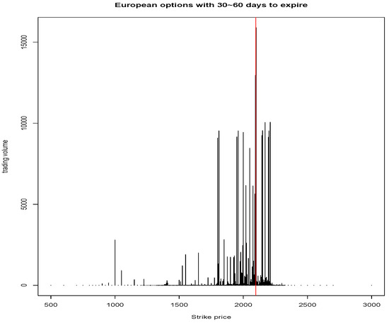
Figure 1. Trading volume vs. strike price for options traded on 18 August 2015 and expired between 18 September 2015 and 18 October 2015 (the S&P 500 index price traded on 18 August 2015 was $2096.92).

It is clear that options with strike prices close to the S&P 500 index price have a higher trading volume, while options whose strike prices are far from the index price have little or even zero trading volume. In Jiang et al. (2021), only options with a positive volume were kept and 70% of the raw data were discarded. In this study, we want our implied risk-neutral densities to reflect extreme market events and the options with extreme strike prices are sufficiently important in estimating the tail behaviors of the implied densities. Therefore, in this study, we keep the options with zero trading volume and only eliminate the options whose trading volume and bid price are zero.

There are 7,385,062 options in our raw data; after the trading volume and bid price filtration, there are 6,854,864 options left. By keeping options that have more than seven days to maturity, we have 6,500,692 options in our cleaned dataset.

4.2. Empirical Study Regarding NCS and Other Relevant Approaches in the Literature

In this section, we use the European option prices on the S&P 500 index described in Section 4.1 to compare the performance of different methods for estimating the RND. We primarily focus on the nonparametric methods described in Section 2. For comparison, following Jiang et al. (2021), we also include one parametric approach, namely the normal inverse Gaussian (NIG) model. According to the simulation studies by Eriksson et al. (2009), if the stock price and its volatility are generated via a Heston model (Heston 1993), a commonly used stochastic volatility model for stock price (Hainaut 2022), the NIG model performs well in approximating the RND.

We follow the idea of Lee (2014) by using only OTM options to fit our NCS model since they are more liquid and thus more informative. However, if the purpose of the implied density is to price complex derivatives, it makes more sense to use all available options to fit the model. This strategy allows the resulting density to incorporate more information about the investors’ expectations of the underlying asset in the market.

As suggested by Lee (2014), OTM options are generally more liquid than ITM options and, therefore, are more commonly used for estimating the RND. Following Lee (2014) and Jiang et al. (2021), we treat the observed OTM option prices as the training data to estimate the RND and use the ITM option prices as the testing data to evaluate the performance of the estimated RND. Since the training and testing data are different in nature (due to moneyness), this type of partition is known as a natural partition (see, e.g., Li and Yang (2022)). The corresponding cross-validation procedure also tests the robustness of the implied density. It should be noted that another type of partition, namely random partitions for K-fold cross-validation, is more commonly used for estimating the prediction errors of methods in many other applications (see, e.g., Hastie et al. (2009)).

When fitting the NCS model with OTM options, we need to take care of the boundary conditions. For example, suppose there are five distinct strike prices $K_1,K_2,K_3,K_4,K_5$ and the distinct OTM option strike prices are $K_2,K_3,K_4$. When deciding the support of the implied density, we use $[log{K}_1-log{b}_1,log{K}_5+log{b}_2]$ instead of $[log{K}_2-log{b}_1,log{K}_4+log{b}_2]$. The values of $b_1$ and $b_2$ are determined by numerical validations.

We numerically examine the performance of the proposed natural cubic spline method (NCS), as well as the normal inverse Gaussian (NIG, Eriksson et al. (2009)), piece-wise constant (PC, Jiang et al. (2021)), uniform quartic B-spline (UQB, Lee (2014)), and cubic spline (CS, Monteiro et al. (2008)) methods in the literature. Following Jiang et al. (2021), we select and sort all available market options into seven categories based on their expiration time, namely, $7\sim 14$ days, $17\sim 31$ days, $81\sim 94$ days, $171\sim 199$ days, $337\sim 393$ days, $502\sim 592$ days, and $670\sim 790$ days. We randomly select 200 cross-sections of options from each expiry category, use the same cross-sections of the data to fit the corresponding model, and then compare their performance in option pricing.

We follow Ghysels and Wang (2014) and define the absolute pricing error $L_a$ and the relative pricing error $L_r$ as follows:

$$\begin{array}{ccc}\hfill L_a& =& \sqrt{{\displaystyle \frac{1}{n}}\sum _{i=1}^n{(V_i^{est}-V_i^{obs})}^2},\hfill \\ \hfill L_r& =& \sqrt{{\displaystyle \frac{1}{n}}\sum _{i=1}^n{\left({\displaystyle \frac{V_i^{est}-V_i^{obs}}{V_i^{obs}}}\right)}^2},\hfill \end{array}$$

where $V^{est}$ denotes the estimated price of the option, and $V^{obs}$ denotes the observed market price of the option. From the investment point of view, both the absolute error and the relative error are important when pricing options.

The results are listed in Table 1 and Table 2. For example, “PC (all+ls)”in “Method” indicates that the PC model is fitted using all the available options and the least square loss function (12), while “NCS (otm+wls)” means that the NCS model is fitted with OTM options only and the weighted least square loss function (13). Columns labeled by $L_a$ or $L_r$ are average pricing errors across 200 randomly selected cross-sections in the corresponding expiry category, and column “200” provides the number out of 200 cross-sections where a risk-neutral density is successfully estimated. Rows labeled by “ITM” (or “OTM”) indicate that the predictions are applied to ITM (or OTM) options only. From Table 1 and Table 2, we can draw the following conclusions:

Table 1. Comparison of five approaches—part 1.

Method		7∼14			17∼31			81∼94			171∼199
		${\mathit{L}}_{\mathit{a}}$	${\mathit{L}}_{\mathit{r}}$	200	${\mathit{L}}_{\mathit{a}}$	${\mathit{L}}_{\mathit{r}}$	200	${\mathit{L}}_{\mathit{a}}$	${\mathit{L}}_{\mathit{r}}$	200	${\mathit{L}}_{\mathit{a}}$	${\mathit{L}}_{\mathit{r}}$	200
NIG	ITM	1.719	0.037	171	2.268	0.037	122	6.128	0.068	38	11.933	0.057	10
	OTM	0.784	1.419	171	1.015	1.212	122	3.477	0.495	38	4.567	0.635	10
UQB	ITM	70.988	0.154	138	69.735	0.155	151	56.973	0.120	113	49.838	0.168	39
	OTM	11.006	374.596	138	16.746	404.313	151	13.086	57.352	113	15.631	14.193	39
CS (ls)	ITM	3.965	0.218	46	1.714	0.043	27	3.235	0.036	39	8.302	0.062	23
	OTM	4.422	13.619	46	1.451	2.164	27	1.292	0.803	39	2.723	0.694	23
CS (wls)	ITM	7.949	0.387	46	3.962	0.123	27	3.665	0.042	39	7.738	0.060	23
	OTM	8.506	22.405	46	3.914	4.243	27	1.205	0.461	39	2.602	0.798	23
PC (all+ls)	ITM	0.253	0.005	198	0.217	0.005	199	0.304	0.002	200	0.288	0.001	197
	OTM	0.251	2.383	198	0.125	0.363	199	0.256	0.290	200	0.204	0.206	197
PC (all+wls)	ITM	0.307	0.006	198	0.307	0.006	197	0.574	0.003	200	0.486	0.002	196
	OTM	0.243	2.321	198	0.090	0.130	197	0.175	0.149	200	0.126	0.045	196
PC (otm+ls)	ITM	0.542	0.013	200	0.591	0.010	200	7.070	0.050	200	8.934	0.050	198
	OTM	0.049	0.211	200	0.067	0.151	200	0.077	0.076	200	0.108	0.073	198
PC (otm+wls)	ITM	1.064	0.019	199	0.761	0.012	200	7.593	0.053	199	9.204	0.051	198
	OTM	0.114	0.128	199	0.097	0.099	200	0.123	0.049	199	0.159	0.048	198
NCS (all+ls)	ITM	0.456	0.022	200	0.224	0.006	200	0.336	0.003	200	0.425	0.003	198
	OTM	0.512	1.133	200	0.135	0.359	200	0.288	0.278	200	0.388	0.220	200
NCS (all+wls)	ITM	3.965	0.056	200	1.895	0.021	200	0.587	0.005	200	0.660	0.006	200
	OTM	0.728	0.239	200	0.235	0.112	200	0.256	0.070	200	0.456	0.075	200
NCS (otm+ls)	ITM	0.950	0.023	200	0.612	0.010	200	5.360	0.039	200	11.979	0.058	200
	OTM	0.413	0.496	200	0.093	0.194	200	0.208	0.157	200	2.594	0.135	200
NCS (otm+wls)	ITM	1.443	0.030	200	0.817	0.012	200	7.074	0.054	200	8.863	0.045	198
	OTM	0.464	0.176	200	0.134	0.117	200	0.352	0.080	200	1.961	0.090	200

Table 2. Comparison of five approaches—part 2.

Method		337∼393			502∼592			670∼790
		${\mathit{L}}_{\mathit{a}}$	${\mathit{L}}_{\mathit{r}}$	200	${\mathit{L}}_{\mathit{a}}$	${\mathit{L}}_{\mathit{r}}$	200	${\mathit{L}}_{\mathit{a}}$	${\mathit{L}}_{\mathit{r}}$	200
NIG	ITM	NA	NA	0	35.179	0.092	4	43.585	0.112	4
	OTM	NA	NA	0	11.802	1.424	4	16.178	0.784	4
UQB	ITM	21.509	0.170	10	37.955	0.134	3	34.048	0.103	5
	OTM	20.676	0.777	10	5.648	0.074	3	7.564	0.061	5
CS (ls)	ITM	19.146	0.129	25	30.889	0.186	23	33.534	0.245	26
	OTM	9.484	0.825	25	14.695	0.448	23	18.586	0.400	26
CS (wls)	ITM	22.294	0.160	24	30.101	0.181	23	33.484	0.277	24
	OTM	13.831	0.881	24	13.297	0.570	23	15.849	0.420	24
PC (all+ls)	ITM	1.003	0.003	199	0.665	0.003	200	0.710	0.003	200
	OTM	0.425	0.198	199	0.588	0.256	200	0.589	0.265	200
PC (all+wls)	ITM	1.281	0.003	199	1.182	0.004	200	1.191	0.003	200
	OTM	0.253	0.033	199	0.356	0.045	200	0.362	0.033	200
PC (otm+ls)	ITM	15.653	0.085	199	20.805	0.086	200	31.661	0.132	200
	OTM	0.273	0.039	199	0.353	0.109	200	0.445	0.034	200
PC (otm+wls)	ITM	15.401	0.084	199	20.277	0.084	200	31.461	0.131	200
	OTM	0.320	0.029	199	0.419	0.036	200	0.510	0.023	200
NCS (all+ls)	ITM	1.361	0.006	200	1.033	0.004	200	2.515	0.010	200
	OTM	1.217	0.207	200	0.948	0.237	200	2.777	0.242	200
NCS (all+wls)	ITM	1.825	0.009	200	1.534	0.006	200	3.910	0.015	200
	OTM	1.285	0.076	200	0.963	0.087	200	2.665	0.098	200
NCS (otm+ls)	ITM	4.056	0.015	200	26.813	0.084	200	5.396	0.015	200
	OTM	1.110	0.119	200	2.454	0.135	200	2.912	0.134	200
NCS (otm+wls)	ITM	8.028	0.034	200	8.604	0.029	200	4.689	0.017	200
	OTM	1.386	0.079	200	1.637	0.084	200	2.150	0.085	200

Note: “NA” appears when the RND is not successfully estimated for any cross-section.

(i)

PC and NCS outperform other methods in terms of computational feasibility. PC and NCS can recover risk-neutral densities for more than 99% of cross-sections from each expiry range. NIG can recover risk-neutral densities for at most 86% of cross-sections. As the expiry time becomes longer than six months, less than 10% of the cross-sections can be used to obtain a feasible NIG model. The reason is that the NIG model has an issue of feasible domain coverage, which becomes more severe as the expiry time increases. UQB and CS have a similar problem when recovering risk-neutral densities, especially for cross-sections longer than six months. UQB becomes infeasible when we cannot find the optimal number of knots that satisfy the condition that all the estimated OTM option prices fall into their bid-ask quotes. The reason for CS becoming infeasible is the lsei package (Wang et al. 2020) used in R software is not capable of finding the solutions for some constrained quadratic programming problems.

(ii)

When comparing our NCS method with the continuous historical methods, the NCS model fitted with OTM options outperforms its competitors in the average pricing accuracy of both OTM and ITM options, especially for the expiry range where the optimization feasibility is comparable.

(iii)

For comparison between PC and NCS in terms of option pricing accuracy, when we use OTM options to fit the risk-neutral density and evaluate the model with weighted least square loss function, that is, OTM+wls, NCS does a much better job in pricing the ITM options for cross-sections with an expiration longer than six months. In other words, for cross-sections longer than six months, the risk-neutral densities restored by NCS are more robust than PC’s.

(iv)

PC fits a constant line segment between every two adjacent knots, and the resulting density is discontinuous throughout the entire domain. On the contrary, NCS can construct implied densities that are desirably twice continuously differentiable. We further illustrate this difference by plotting the risk-neutral densities produced by NCS and PC in Figure 2 and Figure 3 using all the OTM options priced on 25 September 2009 with 187 days to expire.

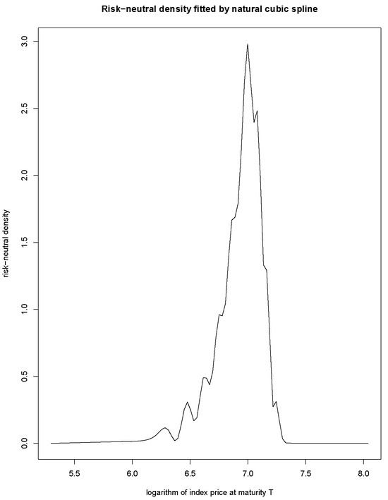Figure 2. RND with NCS method.

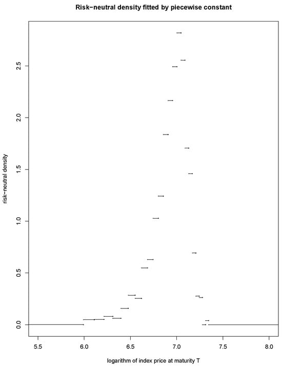Figure 3. RND with PC method.

4.3. Numerical Justification on Consistency of NCS

In this section, we run a simulation study to verify the consistency property of the NCS method, assuming that the true RND follows a normal inverse Gaussian distribution. First, we use options observed on 3 December 2014 with maturity on 2 January 2015 to fit the normal inverse Gaussian model. Next, we generate logarithmically equidistant strike prices and their corresponding put and call option prices. Then, we apply our NCS method and calculate the value of the loss function $F_{\Delta }$. As we increase the number of distinct strike prices and decrease the distance between adjacent log strike prices, we expect to see a decrease in the loss function.

Table 3 shows that as the number of distinct strike prices increases and the distance between adjacent log strikes decreases, the value of the loss function $F_{\Delta }$ decreases to zero.

Table 3. Simulation results for different sets of strike prices.

Run	Number of Distinct Strikes	Distance Between Adjacent Log Strikes	${\mathit{F}}_{\Delta }$
1	8	0.0777	426.74
2	18	0.0388	7.38
3	40	0.0194	0.01
4	88	0.0097	1.33 $\times {10}^{-5}$

For the four different sets of strike prices in Table 3, we plot the fitted NCS model against the true risk-neutral density (“org”) in Figure 4. The results show that the fitted natural cubic spline density converges to the true density as the number of distinct strikes increases, achieving non-negativity and unity integration asymptotically.

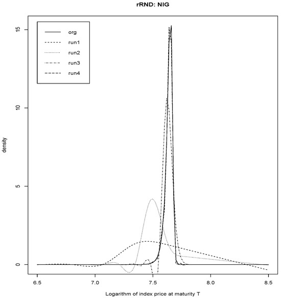
Figure 4. Simulated risk-neutral density plot.

5. Discussion

Risk-neutral density can be characterized using market options. In Section 2.4, we propose a nonparametric natural cubic spline (NCS) approach to model the risk-neutral density through available market options. Unlike the piece-wise constant approach, the implied density from the natural cubic spline is twice continuously differentiable with stable linear tails at both ends (see Figure 2).

According to our empirical study conducted in Section 4.2, when comparing the NCS method with the normal inverse Gaussian method, uniform quartic B-spline method, and cubic spline method, which also generate continuous risk-neutral densities, the NCS method demonstrates superior optimization feasibility. Actually, the NCS approach can recover risk-neutral densities from more than 99% of the cross-sections of options regardless of their expiry time, while the other approaches can recover risk-neutral densities from at most 86% of the cross-sections of options (see Table 1 and Table 2). Additionally, when fitted with OTM options, the NCS method outperforms its competitors in pricing both OTM and ITM options, especially for the expiry range where the optimization feasibility is comparable.

When comparing the NCS method with the piece-wise constant approach which can only produce discontinuous implied densities (see Figure 3), the NCS method can generate more robust risk-neutral densities for options with an expiration longer than six months.

In Section 3, we prove the consistency of the NCS approach. Under reasonable assumptions about the true risk-neutral distribution, we show that as the range of option strike prices approaches $(0,\infty )$ and the difference between adjacent log strike prices shrinks to 0, the fair prices of options based on the estimated risk-neutral density converge to their market values on average. For simplifying the notation, we utilize equidistant log strike prices, while the key property of meshes is actually $\left|\right|\Delta \left|\right|\to 0$. The consistency property is also verified numerically in Section 4.3.

As another important application in practice, the estimated RND can be used to detect potential arbitrage opportunities arising from market prices of options that temporarily violate put-call parity, monotonicity, or strict convexity (Monteiro et al. 2008). As illustrated in Jiang et al. (2021), one can use leave-one-out cross-validation to check if any market prices of options are significantly higher or lower than the fair price provided by the estimated RND, which may indicate profitable opportunities. To capture such opportunities in real-time, one needs high-speed internet, efficient algorithms, and high-performance computers (Kumar and Kumar 2023; Monteiro and Santos 2023).

The proposed method for estimating the RND is applicable only for a given option expiry date. In the literature, many efforts have been made to estimate option price surfaces and state-price densities under no-arbitrage constraints across both strikes and expiry dates. We refer readers to Fengler and Hin (2015), Kundu et al. (2024), and references therein.

References

- Ahlberg, J. Harold, Edwin N. Nilson, and Joseph L. Walsh. 1967. The Theory of Splines and Their Applications. New York and London: Academic Press. [Google Scholar]
- Aït-Sahalia, Yacine, and Andrew W. Lo. 1998. Nonparametric estimation of state-price densities implicit in financial asset prices. Journal of Finance 53: 499–547. [Google Scholar] [CrossRef]
- Aït-Sahalia, Yacine, and Andrew W. Lo. 2000. Nonparametric risk management and implied risk aversion. Journal of Econometrics 94: 9–51. [Google Scholar] [CrossRef]
- Björk, Tomas. 2009. Arbitrage Theory in Continuous Time. New York: Oxford University Press. [Google Scholar]
- Black, Fischer, and Myron Scholes. 1973. The pricing of options and corporate liabilities. Journal of Political Economy 81: 637–54. [Google Scholar] [CrossRef]
- Bliss, Robert R., and Nikolaos Panigirtzoglou. 2002. Testing the stability of implied probability density functions. Journal of Banking & Finance 26: 381–422. [Google Scholar]
- Bondarenko, Oleg. 2003. Estimation of risk-neutral densities using positive convolution approximation. Journal of Econometrics 116: 85–112. [Google Scholar] [CrossRef]
- Breeden, Douglas T., and Robert H. Litzenberger. 1978. Prices of state-contingent claims implicit in option prices. Journal of Business 51: 621–51. [Google Scholar] [CrossRef]
- Buchen, Peter W., and Michael Kelly. 1996. The maximum entropy distribution of an asset inferred from option prices. Journal of Financial and Quantitative Analysis 31: 143–59. [Google Scholar] [CrossRef]
- Campa, José M., P. H. Kevin Chang, and Robert L. Reider. 1998. Implied exchange rate distributions: Evidence from otc option markets. Journal of International Money and Finance 17: 117–60. [Google Scholar] [CrossRef]
- Cox, John C., and Stephen A. Ross. 1976. The valuation of options for alternative stochastic processes. Journal of Financial Economics 3: 145–66. [Google Scholar] [CrossRef]
- Eriksson, Anders, Eric Ghysels, and Fangfang Wang. 2009. The normal inverse gaussian distribution and the pricing of derivatives. Journal of Derivatives 16: 23. [Google Scholar] [CrossRef]
- Fengler, Matthias R., and Lin-Yee Hin. 2015. Semi-nonparametric estimation of the call-option price surface under strike and time-to-expiry no-arbitrage constraints. Journal of Econometrics 184: 242–61. [Google Scholar] [CrossRef]
- Figlewski, Stephen. 2018. Risk-neutral densities: A review. Annual Review of Financial Economics 10: 329–59. [Google Scholar] [CrossRef]
- Ghysels, Eric, and Fangfang Wang. 2014. Moment-implied densities: Properties and applications. Journal of Business & Economic Statistics 32: 88–111. [Google Scholar]
- Grünbichler, Andreas, and Francis A. Longstaff. 1996. Valuing futures and options on volatility. Journal of Banking & Finance 20: 985–1001. [Google Scholar]
- Hainaut, Donatien. 2022. Continuous Time Processes for Finance: Switching, Self-Exciting, Fractional and Other Recent Dynamics. Cham: Springer Nature. [Google Scholar]
- Hastie, Trevor, Robert Tibshirani, and Jerome H. Friedman. 2009. The Elements of Statistical Learning: Data Mining, Inference, and Prediction, 2nd ed. New York: Springer. [Google Scholar]
- Heston, Steven L. 1993. A closed-form solution for options with stochastic volatility with applications to bond and currency options. The Review of Financial Studies 6: 327–43. [Google Scholar] [CrossRef]
- Hull, John C. 2022. Options, Futures, and Other Derivatives, 11th ed. New York: Pearson Education. [Google Scholar]
- Jackwerth, Jens Carsten. 1999. Option implied risk-neutral distributions and implied binomial trees: A literature review. Journal of Derivatives 7: 66–82. [Google Scholar] [CrossRef]
- Jackwerth, Jens Carsten, and Mark Rubinstein. 1996. Recovering probability distributions from option prices. The Journal of Finance 51: 1611–31. [Google Scholar] [CrossRef]
- Jarrow, Robert, and Andrew Rudd. 1982. Approximate option valuation for arbitrary stochastic processes. Journal of Financial Economics 10: 347–69. [Google Scholar] [CrossRef]
- Jiang, Liyuan, Shuang Zhou, Keren Li, Fangfang Wang, and Jie Yang. 2021. A new nonparametric estimate of the risk-neutral density with applications to variance swaps. Frontiers in Applied Mathematics and Statistics 6: 611878. [Google Scholar] [CrossRef]
- Kumar, Abhimanyu, and Sumit Kumar. 2023. Novel computational technique for the direct estimation of risk-neutral density using call price data quotes. Computational and Applied Mathematics 42: 270. [Google Scholar] [CrossRef]
- Kumar, Sudarshan, Sobhesh Kumar Agarwalla, Jayanth R. Varma, and Vineet Virmani. 2023. Harvesting the volatility smile in a large emerging market: A dynamic nelson-siegel approach. Journal of Futures Markets 43: 1615–44. [Google Scholar] [CrossRef]
- Kundu, Arindam, Sumit Kumar, and Nutan Kumar Tomar. 2024. A semi-closed form approximation of arbitrage-free call option price surface. Computational Economics 63: 1431–57. [Google Scholar] [CrossRef]
- Lee, Seung Hwan. 2008. Three Essays on Estimation of Risk Neutral Measures Using Option Pricing Models. Ph.D. thesis, The Ohio State University, Columbus, OH, USA. [Google Scholar]
- Lee, Seung Hwan. 2014. Estimation of risk-neutral measures using quartic b-spline cumulative distribution functions with power tails. Quantitative Finance 14: 1857–79. [Google Scholar] [CrossRef]
- Li, Keren, and Jie Yang. 2022. Score-matching representative approach for big data analysis with generalized linear models. Electronic Journal of Statistics 16: 592–635. [Google Scholar] [CrossRef]
- Li, Yifan, Ingmar Nolte, and Manh Cuong Pham. 2024. Parametric risk-neutral density estimation via finite lognormal-weibull mixtures. Journal of Econometrics 241: 105748. [Google Scholar] [CrossRef]
- Malz, Allan M. 1997. Estimating the probability distribution of the future exchange rate from option prices. Journal of Derivatives 5: 18–36. [Google Scholar] [CrossRef]
- Markose, Sheri, and Amadeo Alentorn. 2005. Option pricing and the implied tail index with the generalized extreme value (gev) distribution. In Computing in Economics and Finance. Cham: Springer Nature, pp. 1–29. [Google Scholar]
- Markose, Sheri, and Amadeo Alentorn. 2011. The generalized extreme value distribution, implied tail index, and option pricing. Journal of Derivatives 18: 35–60. [Google Scholar] [CrossRef]
- Melick, William R., and Charles P. Thomas. 1997. Recovering an asset’s implied pdf from option prices: An application to crude oil during the gulf crisis. Journal of Financial and Quantitative Analysis 32: 91–115. [Google Scholar] [CrossRef]
- Monteiro, Ana M., and António A. F. Santos. 2023. Parallel computing in finance for estimating risk-neutral densities through option prices. Journal of Parallel and Distributed Computing 173: 61–69. [Google Scholar] [CrossRef]
- Monteiro, Ana Margarida, Reha H. Tütüncü, and Luís N. Vicente. 2008. Recovering risk-neutral probability density functions from options prices using cubic splines and ensuring nonnegativity. European Journal of Operational Research 187: 525–42. [Google Scholar] [CrossRef][Green Version]
- Pascucci, Andrea. 2011. PDE and Martingale Methods in Option Pricing. New York: Springer. [Google Scholar]
- Ritchey, Robert J. 1990. Call option valuation for discrete normal mixtures. Journal of Financial Research 13: 285–96. [Google Scholar] [CrossRef]
- Rosenberg, Joshua V. 1998. Pricing multivariate contingent claims using estimated risk–neutral density functions. Journal of International Money and Finance 17: 229–47. [Google Scholar] [CrossRef]
- Rubinstein, Mark. 1994. Implied binomial trees. The Journal of Finance 49: 771–818. [Google Scholar] [CrossRef]
- Shimko, David. 1993. Bounds of probability. Risk 6: 33–37. [Google Scholar]
- Söderlin, Paul. 2000. Market expectations in the uk before and after the erm crisis. Economica 67: 1–18. [Google Scholar] [CrossRef][Green Version]
- Stutzer, Michael. 1996. A simple nonparametric approach to derivative security valuation. Journal of Finance 51: 1633–52. [Google Scholar] [CrossRef]
- Wang, Yong, Charles L. Lawson, and Richard J. Hanson. 2020. lsei: Solving Least Squares or Quadratic Programming Problems Under Equality/Inequality Constraints. R Package Version 1.3-0. Vienna: R Foundation for Statistical Computing. [Google Scholar]
Disclaimer/Publisher’s Note: The statements, opinions and data contained in all publications are solely those of the individual author(s) and contributor(s) and not of MDPI and/or the editor(s). MDPI and/or the editor(s) disclaim responsibility for any injury to people or property resulting from any ideas, methods, instructions or products referred to in the content. |
© 2024 by the authors. Licensee MDPI, Basel, Switzerland. This article is an open access article distributed under the terms and conditions of the Creative Commons Attribution (CC BY) license (https://creativecommons.org/licenses/by/4.0/).