Conditioned Sequence Models for Warm-Starting Sequential Convex Trajectory Optimization in Space Robots

Abstract

Future in-orbit servicing missions, such as spacecraft capture, repair, and assembly, demand robotic systems capable of autonomously computing dynamically feasible, constrained trajectories in real time. Sequential Convex Programming (SCP) has emerged as an effective method for online trajectory optimization in these resource-constrained settings, addressing nonconvex problems through iterative refinement while maintaining the formal guarantees essential for safety-critical applications. While emerging machine learning (ML) methods offer potential enhancements to trajectory generation, they often lack these rigorous guarantees. To address this, we propose a hybrid trajectory optimization framework for robotic servicers, using autoregressive trajectory-generator networks to produce high-quality initial guesses and warm-start an SCP module, enabling the system to produce optimal trajectories quickly and reliably. A key advantage of this approach is the elimination of inverse-kinematics optimization for redundant manipulators during both guess generation and subsequent refinement. By conditioning on exogenous inputs shared with the SCP solver, the networks are inherently task- and obstacle-aware, yielding a tightly integrated architecture that minimizes on-board computational requirements. Results demonstrate that this network-based warm-starting strategy substantially accelerates trajectory generation, reducing both SCP computational time and iterations, while preserving the theoretical guarantees of convex optimization.

1. Introduction

Given the operational complexities of upcoming In-Orbit Servicing (IOS) activities, future missions envision the use of free-flying servicer spacecraft equipped with high-degree-of-freedom (DoF) redundant manipulators, indispensable for performing tasks that are beyond the reach of simpler architectures. These systems will provide the necessary autonomy, versatility, dexterity, and multi-mission capabilities, directly addressing the criticalities unique to such operations. Nevertheless, deploying high-DoF robotic systems for manipulation in confined spaces, while guaranteeing operational safety in dynamic and uncertain environments, remains a significant challenge. Such operations require the servicer to autonomously compute state and control trajectories in real time to complete its mission safely. Specifically, trajectory planning for manipulators with redundant degrees of freedom enables the satisfaction of secondary objectives and constraints, such as collision and singularity avoidance. Despite these advantages, generating feasible and efficient trajectories for redundant systems in space imposes a heavy computational burden. The highly coupled nature of the robotic system renders the inverse kinematics and trajectory optimization problems inherently nonlinear and high-dimensional, leading to nonconvex Optimal Control Problems (OCP) that are difficult to solve in real time on resource-constrained flight hardware. To address these complexities, the literature has applied two distinct approaches: classic trajectory optimization and, more recently, learning-based methods. On the one hand, local optimization methods such as Sequential Convex Programming (SCP) have emerged as effective tools for online trajectory generation. At each iteration, the original problem is convexified and solved efficiently using a convex solver, yielding a solution that is globally optimal for the resulting subproblem. Although these methods are local, meaning they do not guarantee global optimality for the original nonconvex problem, they do ensure convergence to a stationary point under suitable conditions, depending on the quality of the initial guess. For completeness, it should be noted that SCP does not guarantee convergence from an arbitrary initialization; consequently, generating high-quality warm starts for the sequence of convex subproblems is essential. Despite these theoretical limitations, SCP has demonstrated strong empirical reliability, even for highly constrained nonconvex optimal control problems. The global optimality of each convex subproblem, combined with polynomial-time solvability and the local validity of the linear approximations, enables consistent descent of the objective function and progressive satisfaction of the constraints, properties that are essential for applicability within safety-critical tasks. On the other hand, data-driven approaches employing Machine Learning (ML) have demonstrated the ability to generate solutions rapidly, with recent advancements in sequence modeling effectively allowing to predict and control the motion of complex systems. Yet, purely learning-based methods often lack rigorous guarantees with respect to dynamic consistency of the generated trajectories, constraint satisfaction, and optimality. Moreover, the integration of standalone ML methods within spacecraft guidance and control architectures is currently not feasible, primarily due to issues broadly referred to as network explainability. In particular, the absence of established certification processes for such systems, together with the lack of comprehensive verification and validation workflows for algorithms that are inherently difficult to interpret and largely black-box in nature, represents one of their main limitations. As a result, their application to safety-critical IOS tasks remains severely constrained. To address these challenges, state-of-the-art research is increasingly focused on recovering formal guarantees by adopting hybrid algorithms, in which established classical methodologies are employed to verify and refine the outputs produced by ML modules. This hybrid paradigm currently represents one of the most actively investigated directions in the field. Specifically within spacecraft trajectory generation, ML models are leveraged to rapidly generate pseudo-optimal trajectory guesses, which are then used to warm-start optimization solvers. The solvers subsequently apply only minor refinements, thereby significantly reducing the overall computational burden while recovering the safety guarantees for space applications.

1.1. Background on Trajectory Generation in Robotics

Path-planning algorithms in robotics typically compute collision-free geometric paths from a start to a goal configuration, often neglecting system dynamics and control constraints [1,2]. Classical graph-based search methods, such as A*, and sampling-based approaches, like Probabilistic Roadmap (PRM) and Rapidly-exploring Random Tree (RRT), suffer from poor scalability in high-dimensional spaces and generally fail to guarantee dynamic feasibility; moreover, sampling-based methods typically lack optimality guarantees. Since they require no initialization, these planners are frequently used to generate coarse, first-guess trajectories for downstream optimization. Although extensions such as RRT*, PRM*, and kinodynamic RRT* provide asymptotic optimality and account for dynamic constraints, they are generally too computationally demanding for online re-planning in dynamic environments. To address these limitations, motion planning frameworks aim to enforce kinodynamic consistency and retrieve time-parametrized trajectories, elements that are essential for space manipulation tasks. Optimization-based approaches such as CHOMP, STOMP, and TrajOpt [3,4,5] have emerged as strong solutions for high-DoF manipulators in cluttered environments. However, these methods remain sensitive to initialization and often lack hard constraint guarantees or strict dynamic feasibility.

Moving toward real-time control, Model Predictive Control (MPC) has established itself as a leading methodology for the constrained control of complex dynamical systems across varying domains [6,7]. In particular, MPC enables simultaneous planning and control by solving trajectory optimization problems online over a receding time horizon while enforcing constraints, thereby allowing systems to actively react to disturbances. While general Nonlinear Programming (NLP) techniques can be employed within MPC to handle the inherent nonlinearities of robotic systems, an approach falling under the umbrella of Nonlinear MPC (NMPC), their real-time deployment is hindered by substantial computational demands and the absence of strong convergence guarantees. These limitations pose significant risks for safety-critical and resource-constrained applications. To overcome these challenges, convex methods [8,9] have been developed to rapidly compute locally optimal solutions. Among these, SCP [10,11] stands out as one of the most promising methods for real-time applications: the nonconvex problem is successively approximated into a series of convex subproblems, enabling the use of state-of-the-art convex solvers to achieve fast and reliable convergence. This approach significantly enhances computational efficiency and optimization reliability, with proven guarantees of convergence to at least a stationary point. For instance, SCP is applied in [12] to a free-flying space robot to generate optimal, collision-free paths that satisfy manipulator joint constraints. In that work, an inverse kinematics solution is used to initialize the final joint configuration, which is then kept fixed during the optimization. However, the resulting convex problem is solved without explicit obstacle or terminal end-effector constraints. Similarly, SCP is used in [13] to optimize spacecraft-manipulator capture maneuvers, demonstrating real-time feasibility despite nonlinear dynamics. These works highlight the ability of SCP to retain key nonlinearities, while offering the reliable convergence properties suitable for safety-critical space applications, rendering it preferable to general NLP methods in real-time contexts.

Recently, ML techniques have demonstrated significant potential for real-time trajectory generation in ground and space-based manipulators. In this context, Deep Reinforcement Learning (DRL) provides a learning-from-experience framework [14] for developing task- and constraint-aware policies [15,16] in problems formulated as a Markov Decision Process (MDP). These policies effectively handle highly coupled systems and uncertain, unmodeled environments. A primary benefit of this approach is its ability to derive highly adaptive policies that can handle both nominal and off-nominal conditions such as joint failures [17], without re-training. Recent works have also reframed the sequential decision-making problem of an MDP as a conditional sequence modeling problem [18]. In this context, strategies such as offline Reinforcement Learning (RL) are applied to trajectory generation [19], where the agent learns solely from a fixed dataset of pre-computed trajectories (both optimal and suboptimal) without actively interacting with the environment. However, purely ML-based approaches face challenges, most notably the lack of hard guarantees on constraint satisfaction, which is essential for safety-critical applications.

To address these limitations, there is growing interest in hybrid frameworks that integrate data-driven methods with classical techniques [20]. These frameworks aim to achieve real-time performance in resource-constrained applications while preserving theoretical guarantees, which are fundamental in safety-critical operations. For instance, ref. [21] employ a generative model that learns near-optimal policies from offline data, significantly reducing solution time while maintaining constraint compliance. Similarly, ref. [22] use a neural network to warm-start GuSTO [23] for a free-floating robot on the ISS, reducing both the time and iterations required for convergence. Furthermore, ref. [24] propose a transformer-based architecture integrated into an MPC scheme, using a pre-trained network to generate initial trajectory estimates and adaptive terminal costs to ensure hard constraint satisfaction in quadrotor and spacecraft rendezvous tasks. While transformer models are at the forefront of the state-of-the-art, they are often computationally and memory intensive, which can hinder on-board deployment and motivates the study of lighter-weight alternatives.

1.2. Overview

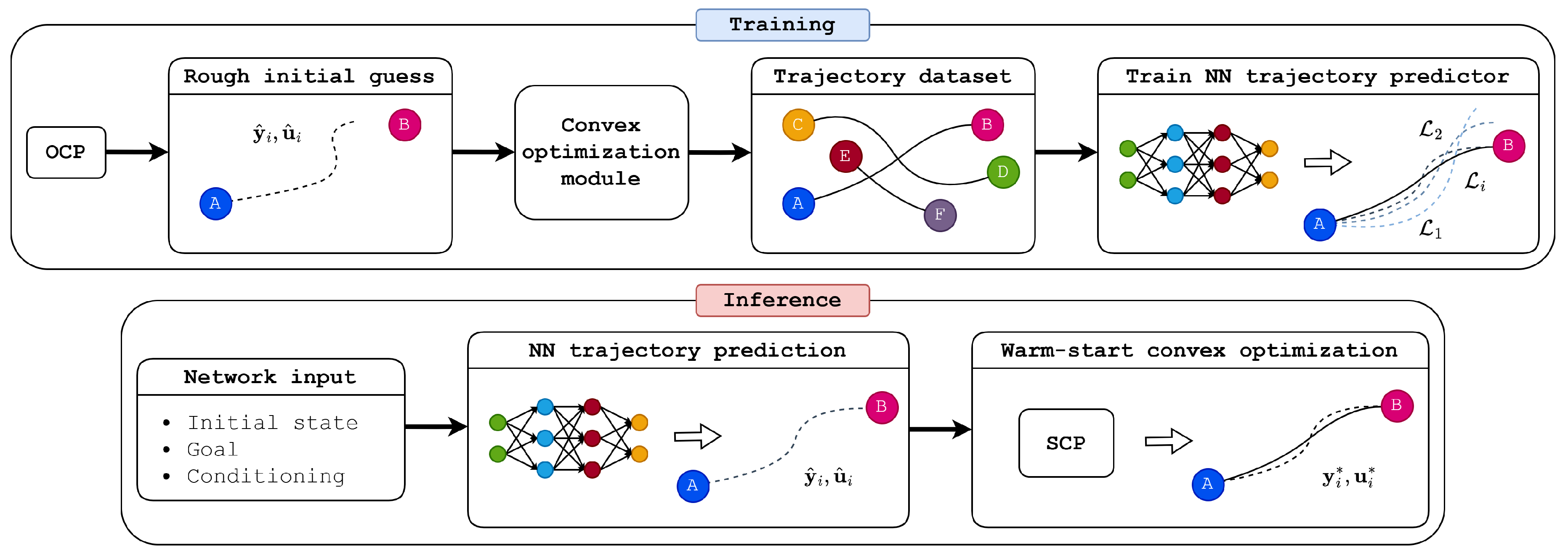
This study presents a hybrid trajectory optimization framework (Figure 1) for free-flying space robots with redundant manipulators. The proposed approach employs an ML-based initial-guess generator to warm-start a subsequent SCP refinement module, enabling fast online trajectory generation and re-planning. First, an SCP formulation tailored to space robot trajectory generation is developed, including an optimal control cost objective, goal-set constraints on the end-effector target pose, and obstacle avoidance constraints. This formulation accommodates systems with free-flying bases and redundant manipulators without requiring an explicit solution to the inverse kinematics problem. To address potential infeasibility of the convex subproblems, penalty terms are also introduced in the objective, allowing the solution to iteratively converge toward optimality even when initialized with low-quality guesses, such as trajectories that do not reach the desired target or that violate constraints. This property is exploited to generate a dataset of optimal trajectories starting from low-quality, often constraint-violating guesses generated via a simple computed-torque controller, with each convex subproblem solved through Gurobi [25]. Leveraging concepts from ML-based sequence modeling, a set of lightweight, conditional autoregressive networks is trained and compared firstly in an obstacle-free environment. By conditioning on inputs exogenous to the trajectory parametrization, such as the end-effector target pose and obstacle locations, the models achieve task- and constraint-aware trajectory generation. They provide high-quality initial guesses to the SCP module, which subsequently guarantees dynamic feasibility and hard constraint satisfaction. Finally, the best-performing network is trained for trajectory generation in the presence of obstacles, demonstrating its ability to incorporate environmental constraints into the generation. The proposed approach combines the adaptability and generative capabilities of data-driven models with the reliability of convex optimization, making it well-suited for on-board use in safety-critical applications like close-proximity manipulation.

The remainder of this paper is organized as follows: Section 2 formulates the Optimal Control Problem (OCP) tailored for space robots and details its convex relaxation into an SCP framework, concluding with the generation of the trajectory datasets. Section 3 describes the implementation of the autoregressive neural networks, specifically addressing the conditioning mechanism, network architectures, and the training strategy employed for the sequence models. Section 4 presents the main results, evaluating the trade-offs between different network variants and demonstrating the computational efficiency gains achieved through the proposed warm-starting strategy. Finally, Section 5 provides concluding remarks and directions for future work.

2. Optimal Control Problem Formulation

The considered scenario involves trajectory generation for a redundant space robot tasked with guiding its end-effector from an initial configuration to a target pose. Given the initial system state $\mathbf{y}\left(t_0\right)$, the desired end-effector pose ${\mathit{\varphi }}_{\mathrm{ee}}^{*}$, and a fixed final time $t_f$, the objective is to determine the optimal sequence of states $\mathbf{y}\left(t_i\right)\in {\mathbb{R}}^n$ and controls $\mathbf{u}\left(t_i\right)\in {\mathbb{R}}^m$ over the time horizon $T=[0,t_f]$. This horizon is divided into N discrete time instants $t_i$ with uniform spacing $\mathrm{\Delta }t$. To simplify notation for quantities evaluated at these instants, indices are used such that ${\mathit{y}}_i\triangleq \mathit{y}\left(t_i\right)$. The trajectory optimization problem is formulated generically in Equations (1a)–(1g) as a discrete-time OCP with a standard finite-horizon additive-cost optimal control objective [26].

$$\begin{array}{cc}\hfill \underset{\mathbf{y},\mathbf{u}}{min}& \mathcal{J}=l_f\left({\mathit{y}}_f\right)+\sum _{i=1}^{N-1}l({\mathit{y}}_i,{\mathit{u}}_i)\hfill \\ \hfill \mathrm{subject}\mathrm{to}\end{array}$$

(1a)

$$\begin{array}{ccc}\hfill & {\mathbf{y}}_{i+1}=\mathbf{f}({\mathbf{y}}_i,{\mathbf{u}}_i)\hfill & \hfill \forall i\in [0,\dots ,N-2]\end{array}$$

(1b)

$$\begin{array}{cc}\hfill & \mathbf{y}\left(t_0\right)={\mathbf{y}}_0\hfill \end{array}$$

(1c)

$$\begin{array}{cc}\hfill & |{\mathit{\varphi }}_{\mathrm{ee}}\left({\mathbf{y}}_f\right)-{\mathit{\varphi }}_{\mathrm{ee}}^{*}|\le {\epsilon }_{\mathrm{tol}}\hfill \end{array}$$

(1d)

$$\begin{array}{ccc}\hfill & d_{mji}\ge d_{\min }\hfill & \hfill \forall m,j,i\end{array}$$

(1e)

$$\begin{array}{ccc}\hfill & {\mathbf{y}}_{\min }\le {\mathbf{y}}_i\le {\mathbf{y}}_{\max }\hfill & \hfill \forall i\in [0,\dots ,N-1]\end{array}$$

(1f)

$$\begin{array}{ccc}\hfill & {\mathbf{u}}_{\min }\le {\mathbf{u}}_i\le {\mathbf{u}}_{\max }\hfill & \hfill \forall i\in [0,\dots ,N-1]\end{array}$$

(1g)

As will be detailed in the following sections, this OCP is both nonlinear and nonconvex, and is subjected to the following constraints: space robot dynamics (Equation (1b)), initial state (Equation (1c)), end-effector terminal pose (Equation (1d)), collision avoidance (Equation (1e)), and state and control bounds (Equations (1f) and (1g)). The constraint terms and objective cost are detailed in Section 2.1 and Section 2.2 together with their convex relaxation, and the complete convex subproblem solved at each SCP iteration is provided in Section 2.3.

2.1. Convex Relaxation for SCP

The nonconvex terms in the OCP, specifically Equations (1a), (1b), (1d) and (1e), must be reformulated to fit within the SCP framework. The core principle of SCP is to iteratively transform the original nonconvex problem into a sequence of locally valid and highly tractable convex subproblems, each of which can be efficiently solved to the globally optimal solution. It is emphasized that this notion of global optimality applies to the individual subproblems; the original nonconvex problem can, in general, be solved only up to a stationary point. At each iteration, the convex subproblem is constructed by forming affine approximations of the nonconvex components around the current trajectory estimate. To preserve the local validity of these approximations, a trust region centered at the latest solution is imposed as an additional constraint. This trust-region mechanism ensures the local validity of the approximation, thereby promoting consistent objective descent and progressive constraint satisfaction across iterations. Let ${\mathit{x}}^{\left(k\right)}$ denote the solution estimate at the k-th SCP iteration. A first-order Taylor expansion of the nonconvex terms around ${\mathit{x}}^{\left(k\right)}$ can be generically written as

$$\mathit{g}\left(\mathit{x}\right)\approx \mathit{g}\left({\mathit{x}}^{\left(k\right)}\right)+\nabla \mathit{g}{\left({\mathit{x}}^{\left(k\right)}\right)}^{⊺}(\mathit{x}-{\mathit{x}}^{\left(k\right)})$$

(2)

that is used to retrieve an affine approximation of the vector-valued multivariate function $\mathit{g}(\mathit{x})$. The gradients required for Equation (2) are computed accurately and efficiently through automatic differentiation, using CasADi [27]. This accuracy is crucial for ensuring valid linearizations and preserving the convergence properties of the SCP framework, particularly under highly nonlinear dynamics and constraints. Note that all quantities marked with $\left(k\right)$ in the following sections are pre-computed before the convex solver call to improve efficiency, as they depend solely on the current trajectory reference.

2.1.1. Dynamics Constraint

The system in Equation (1b) is implemented using the open-source SPART toolkit [28]. This toolkit supports Unified Robot Description Format (URDF) inputs, allowing for rapid modification of the underlying dynamics, and provides an accurate representation of a free-flying space robot assumed to be equipped with a single manipulator. For this system, the generalized coordinates are defined as $\mathit{x}=[{\mathit{q}}_0,{\mathit{q}}_m]$, where ${\mathit{q}}_0$ represents the pose of the spacecraft base and ${\mathit{q}}_m$ collects the manipulator joint angles. The corresponding equations of motion are given by $\mathit{H}\left(\mathit{x}\right)\ddot{\mathit{x}}+\mathit{C}(\mathit{x},\dot{\mathit{x}})\dot{\mathit{x}}=\mathit{u}$, where $\mathit{H}$ and $\mathit{C}$ denote the generalized inertia and convective inertia matrices, respectively. To demonstrate the approach, the algorithm is applied to a redundant planar space robot consisting of a 3-DoF actuated base and a 4-DoF manipulator. The physical characteristics of the space robot are provided in

Table 1. Space robot physical characteristics.

Body	Mass ($\mathbf{kg}$)	Type	Length/Offset ($\mathbf{cm}$)	Inertia ($\mathbf{kg}\mathit{·}{\mathbf{m}}^2$)	Axis
Base 0	250	-	$50\times 50$	10.42
Joint 1	-	Revolute	25	-	$Z[0,0,1]$
Link 1	5	-	50	0.11	-
Joint 2	-	Revolute	25	-	$Z[0,0,1]$
Link 2	5	-	50	0.11	-
Joint 3	-	Revolute	25	-	$Z[0,0,1]$
Link 3	5	-	50	0.11	-
Joint 4	-	Revolute	25	-	$Z[0,0,1]$
Link 4	5	-	50	0.11	-
End effector	1	-	-	0.001	-

, where the numbering of elements is sequential from base to end-effector. Regarding the joints, the offset parameter represents the distance with respect to the center of the previous link, while for links the value is representative of dimensions.

Because the dynamics are neither discrete nor convex, they must be adapted for the convex framework. First, the dynamics are reformulated as a first-order ODE system $\dot{\mathit{y}}\left(t\right)=\mathit{f}(\mathit{y},\mathit{u})$. The state vector is defined as $\mathit{y}=[{\theta }_0,{\mathit{r}}_0,{\omega }_0,{\mathit{v}}_0,{\mathit{q}}_m,{\dot{\mathit{q}}}_m]\in {\mathbb{R}}^{14}$. Here, ${\theta }_0$ and ${\omega }_0$ represent the base attitude and angular rate relative to the horizontal axis (positive counter-clockwise), ${\mathit{r}}_0$ and ${\mathit{v}}_0$ denote the base position and velocity, ${\mathit{q}}_m$ and ${\dot{\mathit{q}}}_m$ are the manipulator joint angles and rates, and $\mathit{u}=[{\mathit{u}}_0,{\mathit{u}}_m]\in {\mathbb{R}}^7$ represents the actuation applied to the base and manipulator. The continuous-time space robot dynamics require convexification and discretization to align with the original OCP. By defining $\mathrm{\Delta }t=t_f/(N-1)$ and assuming a zero-order hold control policy, such that $\mathit{u}\left(t\right)=\mathit{u}\left(t_i\right)$$\forall t\in [t_i,t_{i+1})$, the application of a trapezoidal integration scheme yields the resulting affine dynamics directly compatible with SCP:

$${\mathbf{A}}_{i+1}^{\left(k\right)}{\mathbf{y}}_{i+1}-{\mathbf{A}}_i^{\left(k\right)}{\mathbf{y}}_i+{\mathbf{B}}_{i+1}^{\left(k\right)}{\mathbf{u}}_{i+1}+{\mathbf{B}}_i^{\left(k\right)}{\mathbf{u}}_i={\mathbf{d}}_{i+1}^{\left(k\right)}+{\mathbf{d}}_i^{\left(k\right)}\forall i\in [0,\dots ,N-2]$$

(3)

where k is the current iterate of the SCP solution. To avoid cluttered computations, the procedure to retrieve the terms in Equation (3) is presented in Appendix A.1.

2.1.2. End-Effector Terminal Constraint

For redundant manipulators, the inverse kinematics problem is inherently ill-posed and typically lacks closed-form solutions, as a specific end-effector pose can be reached through infinitely many combinations of joint angles [29]. While this introduces complexity for trajectory generation, such redundancy is advantageous in IOS applications, where the redundant DoFs can be exploited to achieve secondary objectives, such as enforcing trajectory constraints. Rather than solving the inverse kinematics problem to enforce a specific joint configuration at the final time, which limits the solution space during optimization of the trajectory, this work employs a more generic terminal constraint. To grant the solver greater flexibility in finding optimal trajectories for the manipulator, the terminal end-effector pose is enforced as a goal-set constraint (Equation (1d)). This allows the solver to freely select the final joint angles, provided the end-effector lies within an acceptable tolerance ${\mathit{\epsilon }}_{\mathrm{tol}}$ of the target pose. For the planar space robot, the end-effector state is defined as ${\mathit{\varphi }}_{\mathrm{ee}}\left(t_i\right)=[\theta ,x,y]=\mathrm{FK}\left({\mathit{y}}_i\right)$, where $\theta$ denotes the orientation relative to the x-axis, and $x,y$ represent the position relative to the origin. Additionally, the function $FK\left(·\right)$ generically represents a forward kinematics solution to compute the end-effector pose from the current configuration. To relax the original nonconvex constraint (Equation (1d)) for compatibility with convex solvers, an affine approximation of the inner term ${\mathit{\varphi }}_{\mathrm{ee}}\left({\mathit{y}}_f\right)$ is sufficient and leads to Equation (4), where all terms are detailed in Appendix A.2.

$$|{\mathbf{A}}_{{\mathit{\varphi }}_{\mathrm{ee}}}^{\left(k\right)}{\mathbf{y}}_f+{\mathbf{C}}_{{\mathit{\varphi }}_{\mathrm{ee}}}^{\left(k\right)}-{\mathit{\varphi }}_{\mathrm{ee}}^{*}|\le {\mathit{\epsilon }}_{\mathrm{tol}}$$

(4)

2.1.3. Collision Avoidance Constraint

The collision avoidance constraint (Equation (1e)) ensures that, at each timestep i, the minimum distance between every point m on the manipulator mesh (including links and joints) and obstacle j, satisfies Equation (5).

$$d_{mji}=\left|\right|{\mathit{P}}_{mi}-{\mathit{P}}_j\left|\right|\ge d_{\min }$$

(5)

This constraint is concave, defining the region outside a sphere, and requires convex relaxation for compatibility with SCP. The obstacles in this work are approximated as spheres, a conservative yet computationally efficient approach for collision checking [5]. 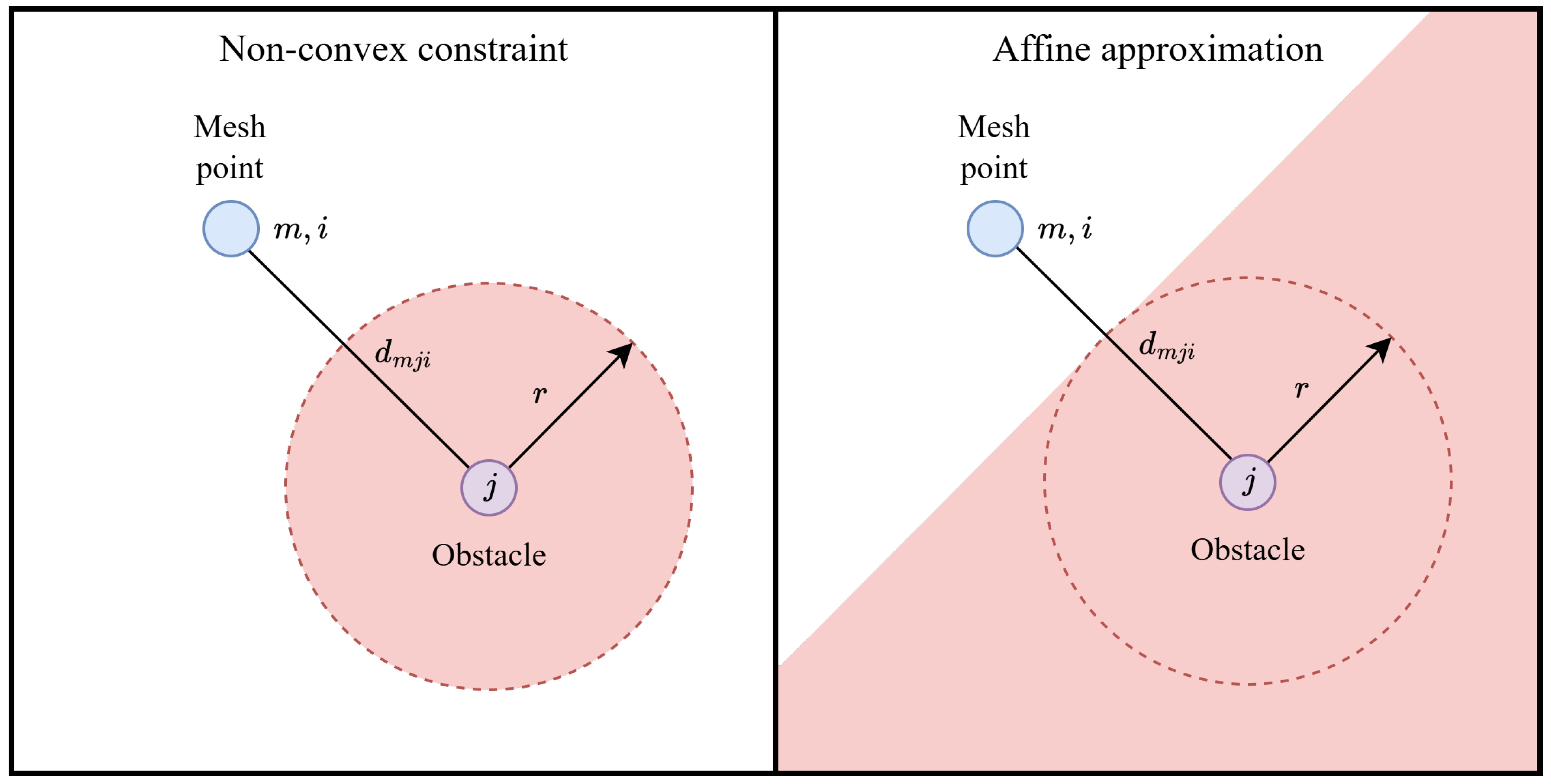Numerous methods [8] have been developed to convexify such constraints, which are common in collision avoidance scenarios ranging from spacecraft keep-out zones and drone swarm coordination to robotic obstacle avoidance [5,30,31]. A standard technique for handling these constraints is the supporting hyperplane method: the obstacle boundary is approximated by a plane tangent to the obstacle and perpendicular to the vector connecting the obstacle center to the point of interest, as shown in Figure 2. While this approach is demonstrated here for spherical obstacles, it readily extends to general nonconvex shapes by introducing an intermediate step that extracts their convex hull, and subsequently applies the supporting hyperplane method as in [5]. Alternative formulations for handling arbitrary obstacle geometries also exist in the literature, including methods based on local surface normals and signed distance fields to obtain the required gradients, as in [32]. The typical trade-offs among these approaches involve balancing computational complexity against the geometric complexity of the obstacles in the environment, as well as choosing an acceptable level of conservatism when approximating or decomposing the obstacles.

To reduce the computational load, a strategy from [5] is applied: constraints between mesh elements m and obstacles j are activated only when the distance in the reference trajectory falls below a specific activation threshold $d^{*}$. This significantly improves efficiency by limiting collision checks to points at highest risk of collision. The resulting affine constraint for the SCP formulation is given in Equation (6), with derivation details provided in Appendix A.3.

$$\begin{array}{ccc}\hfill {\widehat{\mathit{A}}}_{mji}^{\left(k\right)}{\mathit{y}}_i+{\widehat{C}}_{mji}^{\left(k\right)}\ge d_{\min }& \hfill & \hfill \forall m,j,i\mathrm{s}.\mathrm{t}.d_{mji}^{\left(k\right)}<d^{*}\end{array}$$

(6)

2.2. Objective Function

The cost function in Equation (1a), representing a generic finite-horizon optimal control objective [26], is expanded in Equation (7). The implemented objective includes a term for control minimization, along with penalties for end-effector terminal pose and collision violations, that will be detailed in this section.

$$\begin{array}{c}\hfill {\mathcal{J}}_{\mathrm{convex}}=J_{\mathrm{ee}}\left({\mathbf{y}}_f\right)+\sum _{i=1}^{N-1}\left[J_u\left({\mathit{u}}_i\right)+J_{\mathrm{Coll}}\left({\mathit{s}}_{coll,i}\right)\right]\end{array}$$

(7)

First, a smooth quadratic control effort term is defined as $J_u\left({\mathit{u}}_i\right)={\lambda }_u{\mathit{u}}_i^{⊺}{\mathit{u}}_i$. To prevent infeasibility in the convex subproblem when the initial guess is poor (specifically when the end-effector is far from its target), the hard terminal constraint (Equation (4)) is temporarily removed as in [13], in favor of a penalty term. This term is defined as $J_{\mathrm{ee}}={\lambda }_{\mathrm{ee}}{\mathit{s}}_{\mathrm{ee}}^{⊺}{\mathit{s}}_{\mathrm{ee}}$, where ${\mathit{s}}_{\mathrm{ee}}={\mathit{A}}_{{\mathit{\varphi }}_{\mathrm{ee}}}^{\left(k\right)}{\mathit{y}}_f+{\mathit{C}}_{{\mathit{\varphi }}_{\mathrm{ee}}}^{\left(k\right)}-{\mathit{\varphi }}_{\mathrm{ee}}^{*}$ represents a convex residual on the end-effector pose error, derived using the equations in Section 2.1.2. This strategy effectively balances feasibility and optimality within each convex subproblem, promoting faster convergence and allowing the solver to handle initially infeasible guesses. Note that ${\mathit{s}}_{\mathrm{ee}}$ represents solely a residual, not a slack variable, and is therefore not part of the decision vector. Finally, numerical stability is significantly improved by implementing the collision avoidance constraints with a slack variable ${\mathit{s}}_{\mathrm{coll}}$. This maintains problem feasibility by allowing temporary constraint violations, particularly during early iterations when the SCP is initialized with low-quality guesses that may involve collisions. To allow early iterations to progress while driving violations to zero over time, effectively acting as a continuation mechanism, the slack variable is penalized via $J_{\mathrm{coll}}={\lambda }_{\mathrm{coll}}{\mathit{s}}_{\mathrm{coll}}^{⊺}{\mathit{s}}_{\mathrm{coll}}$. Unlike ${\mathit{s}}_{\mathrm{ee}}$, ${\mathit{s}}_{\mathrm{coll}}$ is effectively an optimization variable, requiring a positivity constraint (${\mathit{s}}_{\mathrm{coll}}\ge 0$) to prevent artificial tightening of the collision limits. In this work, the weighting parameters are selected as ${\lambda }_{\mathrm{ee}}={10}^6$, ${\lambda }_{\mathrm{coll}}={10}^6$, and ${\lambda }_{\mathrm{u}}={10}^2$. While more precise tuning of these parameters is possible, the general rationale behind their selection is to overcome infeasible guesses and improve convergence speed. The weights are selected to achieve a two-step improvement of the objective, focusing first on the high-level tasks and then on secondary ones. The provided weights firstly push the guess trajectory towards feasibility and high-level task satisfaction (including the end-effector target and obstacle avoidance), which is why ${\lambda }_{\mathrm{ee}}$ and ${\lambda }_{\mathrm{coll}}$ are set at higher orders of magnitude than ${\lambda }_{\mathrm{u}}$. Once a feasible trajectory is found that can achieve these objectives, a more fine-grained trajectory optimization takes place to reduce the control effort required for its execution, an aspect that is also fundamental to reduce the disturbances experienced at the base of the servicer.

2.3. Complete SCP Algorithm Implementation

The complete formulation of the convexified subproblem, solved at the k-th SCP iteration, is provided in Equations (8a)–(8j). The decision variables comprise the space robot states ${\mathit{y}}_i$, control actions ${\mathit{u}}_i$, and the collision slack variables ${\mathit{s}}_{\mathrm{coll},\mathrm{i}}$. Additionally, to maintain the local validity of the convex approximation, trust region constraints are included as shown in Equations (8i) and (8j). Regarding Equations (8g) and (8h), it is important to note that manipulator joint limits have not been enforced in this work. While the optimization algorithm can easily handle such box constraints, they are omitted due to the inherent restrictiveness of the planar 2D assumption. It was found that enforcing joint limits in this simplified environment significantly constrains the workspace, especially under conditions where obstacles are present, often leading to problem infeasibility when the manipulator has to maneuver around obstacles between the start and goal. This is a structural limitation specific to the 2D case; joint limits will be incorporated in future extensions dealing with full 3D dynamics, and once a more realistic manipulator model or configuration is used, are highly dependent on the selected geometries. Given the effect of these constraints on the trajectories with obstacles, these constraints have also been removed in the trajectories without obstacles, to keep the formulation of the problem consistent under both conditions, for fair comparison in the results. The trust region radii, ${\mathit{\rho }}_y$ and ${\mathit{\rho }}_u$, are updated over the iterations following the adaptation logic described in [33].

$$\begin{array}{cc}\hfill \underset{\mathbf{y},\mathbf{u}}{min}& J_{\mathrm{ee}}\left({\mathit{y}}_f\right)+\sum _{i=1}^{N-1}\left[J_u\left({\mathit{u}}_i\right)+J_{\mathrm{Coll}}\left({\mathit{s}}_{coll,i}\right)\right]\hfill \\ \hfill \mathrm{subject}\mathrm{to}\end{array}$$

(8a)

$$\begin{array}{ccc}\hfill & {\mathbf{A}}_{i+1}^{\left(k\right)}{\mathbf{y}}_{i+1}-{\mathbf{A}}_i^{\left(k\right)}{\mathbf{y}}_i+{\mathbf{B}}_{i+1}^{\left(k\right)}{\mathbf{u}}_{i+1}+{\mathbf{B}}_i^{\left(k\right)}{\mathbf{u}}_i={\mathbf{d}}_{i+1}^{\left(k\right)}+{\mathbf{d}}_i^{\left(k\right)}\hfill & \hfill \forall i\in [0,\dots ,N-2]\end{array}$$

(8b)

$$\begin{array}{cc}\hfill & \mathbf{y}\left(t_0\right)={\mathbf{y}}_0\hfill \end{array}$$

(8c)

$$\begin{array}{cc}\hfill & |{\mathbf{A}}_{{\mathit{\varphi }}_{\mathrm{ee}}}^{\left(k\right)}{\mathbf{y}}_f+{\mathbf{C}}_{{\mathit{\varphi }}_{\mathrm{ee}}}^{\left(k\right)}-{\mathit{\varphi }}_{\mathrm{ee}}^{*}|\le {\mathit{\epsilon }}_{\mathrm{tol}}\hfill \end{array}$$

(8d)

$$\begin{array}{ccc}\hfill & {\widehat{\mathit{A}}}_{mji}^{\left(k\right)}{\mathit{y}}_i+{\widehat{C}}_{mji}^{\left(k\right)}+{\mathit{s}}_{\mathrm{coll}}\ge d_{\min }\hfill & \hfill \forall m,j,i\mathrm{s}.\mathrm{t}.d_{mji}^{\left(k\right)}<d^{*}\end{array}$$

(8e)

$$\begin{array}{cc}\hfill & {\mathit{s}}_{\mathrm{coll}}\ge 0\hfill \end{array}$$

(8f)

$$\begin{array}{ccc}\hfill & {\mathbf{y}}_{\min }\le {\mathbf{y}}_i\le {\mathbf{y}}_{\max }\hfill & \hfill \forall i\in [0,\dots ,N-1]\end{array}$$

(8g)

$$\begin{array}{ccc}\hfill & {\mathbf{u}}_{\min }\le {\mathbf{u}}_i\le {\mathbf{u}}_{\max }\hfill & \hfill \forall i\in [0,\dots ,N-1]\end{array}$$

(8h)

$$\begin{array}{cc}\hfill & |\mathbf{y}-{\mathbf{y}}^{\left(k\right)}|\le {\rho }_y\hfill \end{array}$$

(8i)

$$\begin{array}{cc}\hfill & |\mathbf{u}-{\mathbf{u}}^{\left(k\right)}|\le {\rho }_u\hfill \end{array}$$

(8j)

The convexity of the problem was verified using the CVX disciplined convex programming library [34], which explicitly requires convex expressions as inputs and validates their convexity. However, due to the significant overhead associated with the CVX parsing and problem reformulation routines, consuming approximately 80–85% of the total compute time per iteration, direct calls to Gurobi [25] were preferred for the final implementation. The continuation mechanisms described in Section 2.2, specifically the end-effector penalty and collision slack, guarantee that the convexified sub-problem remains feasible even when those constraints are not respected at the current iterate. This effectively isolates these constraints as the causes of potential solver failure. However, the solver may still report infeasibility, failure, or numerical issues. This section describes the fallback strategies implemented to handle such cases, which are applied to attempt recovery before reporting a final failure in the SCP. The primary mechanism addresses artificial infeasibility. To ensure a valid linear approximation and accelerate convergence of the nonlinear problem, the trust region is initially kept tight. However, if the initial guess is poor, the trust region may not intersect with the feasible region defined by other constraints. If the intersection of these is an empty set, the SCP sub-problem becomes infeasible even though the underlying nonconvex problem may still be feasible. Indeed, the cause of this failure is the formulation of the SCP sub-problem itself, rather than a true infeasibility of the nonconvex problem. To resolve this, the algorithm automatically expands the trust region until the feasible set is non-empty, up to a maximum value, and the problem is re-solved. This approach allows the solver to find a feasible solution at the expense of convergence speed. While this requires additional iterations and computational cost, it is a necessary tradeoff to avoid optimization failure. Crucially, regardless of the trust region value, the solution remains bounded and consistent with the robot’s dynamics, as these are strictly enforced as hard constraints. Simultaneously, the Gurobi NUMERIC_FOCUS parameter is increased for the re-solve attempt, instructing the solver to prioritize numerical stability again at the cost of computational expense. If these mechanisms successfully overcome the infeasibility, the solver parameter is reset, and the trust region adaptation is executed nominally. Note that infeasibility or failure from the Gurobi solver typically occurs only in the first few iterations of the SCP, that is when this recovery typically takes place. If no solution is found despite these fallback measures, the SCP solver returns a failure, indicating that the linear assumption has broken down or the underlying problem is truly infeasible.

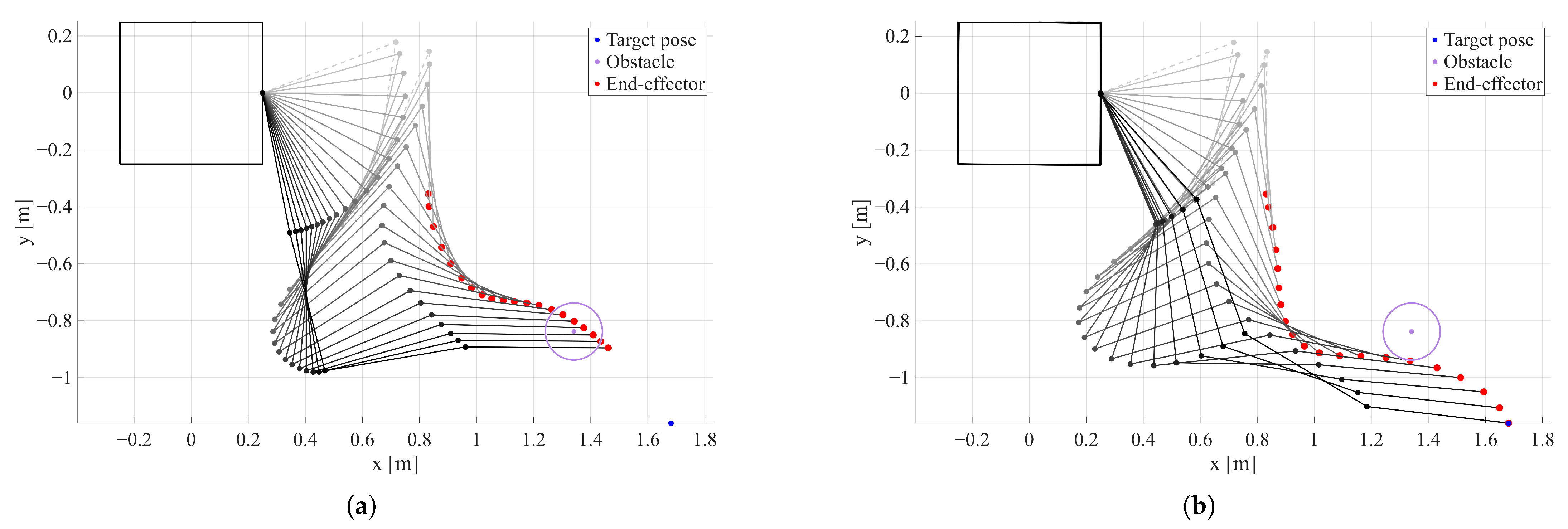
An example of an optimized trajectory is provided in Figure 3; starting from a low-quality initial guess that intersects the obstacle and fails to reach the end-effector target, the method achieves convergence in 12 iterations. On average, a single SCP iteration requires 0.128 s on an i7-11800H laptop CPU, with 0.106 s allocated to the solver and 0.022 s to linearization and matrix preparation. The solution performance, specifically the number of SCP iterations required, can be significantly improved by initializing with high-quality, pseudo-optimal guesses provided by autoregressive trajectory generator networks.

Using the proposed framework, two distinct datasets are generated: one representing an obstacle-free environment and another featuring a single obstacle positioned between the initial and target end-effector poses. For the optimization settings, the maximum number of SCP iterations was set to 30, with $\mathrm{\Delta }t=0.1\mathrm{s}$, $t_f=20\mathrm{s}$, and an obstacle radius of $10\mathrm{cm}$. Each trajectory in the dataset represents a distinct operating condition, generated by randomizing the initial manipulator state, end-effector target, and obstacle locations, and employing a computed-torque control approach to generate the initial guess. The end-effector targets are randomized on the right-hand side of the robot, with coordinates bounded by $x\in [1,2]$ m, $y\in [-1.2,1.2]$ m, and a desired orientation between $[-30,30]$ deg. Given that the base position is controlled to stay in its original location, the reachability of the randomized target is checked to make sure it falls within the workspace of the robot, avoiding trajectories that do not have a solution. The initial manipulator configuration is selected from a set of 38 pre-defined configurations representing various manipulator deployment stages that fall close to the robot; to maximize variability, each joint is further perturbed by a uniform random angle in $[-30,30]$ deg. Finally, obstacles are randomized in the vicinity of the line connecting the initial and final end-effector positions, with a randomized transversal offset. Note that the obstacle location is also checked such that the end-effector target remains valid and reachable (i.e., it the obstacle radius cannot contain the target). Each dataset is populated with 15,000 optimal trajectories; it is worth noting that this sample size is considerably smaller than in related works; for instance, ref. [21] utilizes a test set of 20,000 trajectories, which typically accounts for only about 10% of the full dataset.

3. Autoregressive Network Implementation and Training

The final component required to complete the hybrid trajectory generation approach is a framework for task- and constraint-aware autoregressive neural network architectures. These architectures are designed to rapidly generate pseudo-optimal trajectory guesses to warm-start the SCP optimization, thereby reducing the number of required iterations and lightening the overall computational load of the trajectory generation pipeline. Several variants utilizing stacked Multi-Layer Perceptron (MLP), Long Short-Term Memory (LSTM), Gated Recurrent Unit (GRU), and Transformer layers are compared to identify the most efficient architecture for guess generation, balancing generation accuracy with inference speed and memory requirements.

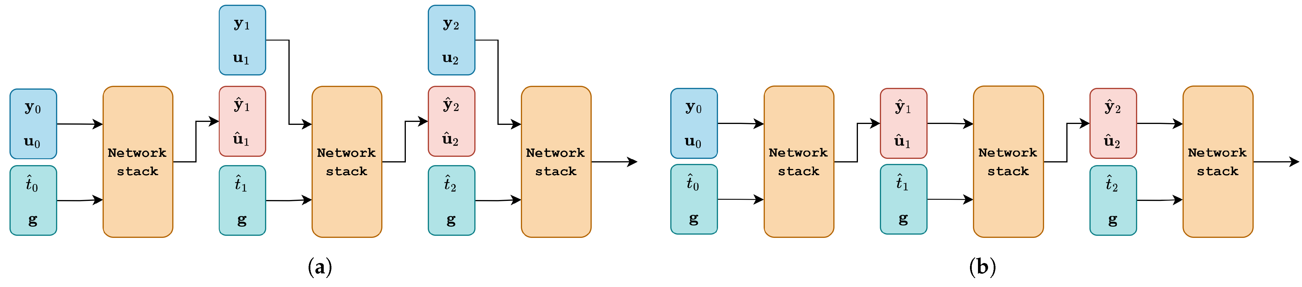
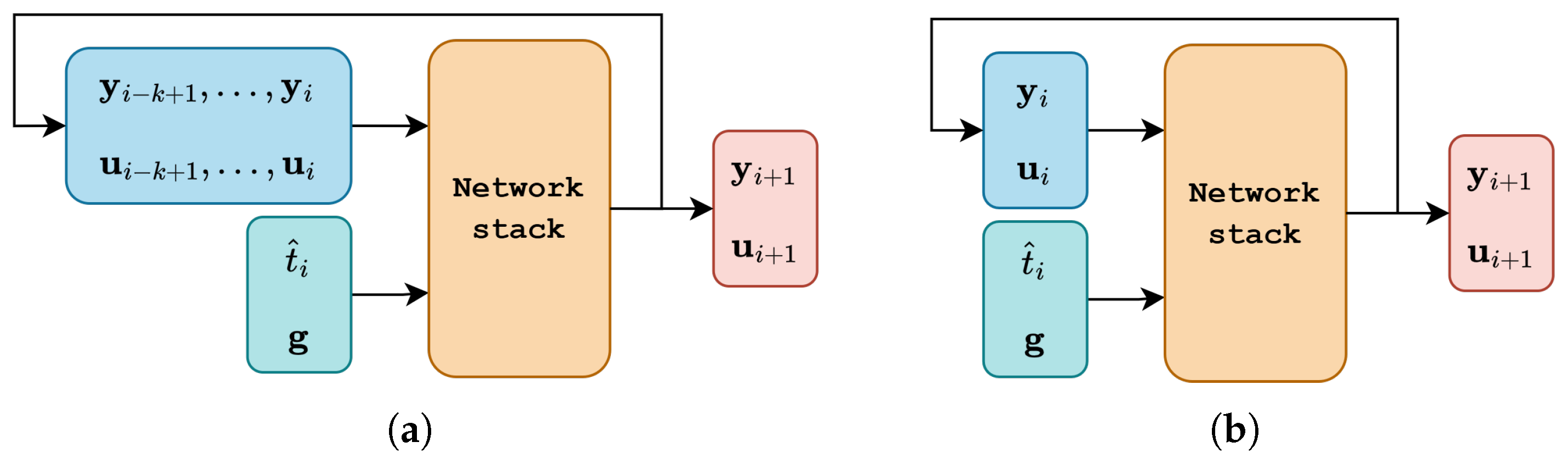
All models share a common input structure comprising three elements: (i) the current system state and control; (ii) a normalized timestep, ${\widehat{t}}_i$, relative to $t_f$; and (iii) a conditioning vector, $\mathit{g}$, that encodes the end-effector target pose and obstacle positions (when present). The generation process begins with the system’s initial conditions. At each autoregressive step i, the network predicts the state and control at time $i+1$ conditioned on $\mathit{g}$; this prediction is then fed back as input for the next step, as shown in Figure 4. This procedure continues until the entire trajectory is inferred, creating an efficient architecture that exploits parameter sharing across timesteps.

Non-recurrent networks do not inherently maintain context from previous timesteps during inference. To address this, the MLP and Transformer models employ a k-step autoregressive scheme [35,36,37], where the input consists of the preceding k timesteps, functioning as a sliding window. While increasing k generally improves generation accuracy due to the greater context provided to the networks, it also increases network size, memory footprint, and inference latency; therefore, this parameter must be carefully tuned. These factors are particularly critical for the Transformer architecture, especially when considering similar approaches for on-board implementation. In contrast, recurrent architectures such as the LSTM and GRU selectively retain long- and short-term context via hidden states and gating mechanisms, eliminating the need to explicitly feed multiple timesteps as input.

A central feature of all proposed architectures is the conditioning mechanism, which enables task and environmental awareness during generation. First, without the conditioning input, the networks would lack fundamental context regarding the OCP goal, biasing outputs toward the model’s statistical priors and yielding unsatisfactory results during generation. By incorporating a conditioning vector, the network instead produces intermediate states and controls consistent with the final OCP goal. This effectively constrains generation to trajectories that approach the prescribed target, even for scenarios unseen during training, a primary objective of the learning process. Second, the conditioning mechanism mitigates error compounding during autoregressive generation, which would otherwise cause rapid divergence of the trajectories. This enables the network to automatically compensate for its own prediction errors, ensuring an effective autoregression.

Autoregressive Network Training

Network and training hyperparameter tuning is initially conducted on the obstacle-free dataset due to the lower complexity of the environment. The networks are trained in PyTorch v2.7 using the AdamW optimizer and a squared-error loss function (Equation (9)) [21,24] for the trajectory generation task. Each model is trained for 6000 epochs with a batch size of 2048, utilizing a cosine-annealed learning rate decaying from ${10}^{-3}$ to ${10}^{-5}$ and a weight decay of ${10}^{-4}$. Consistent with literature on autoregressive and recurrent networks, the models exhibit a strong tendency toward exploding gradients; consequently, gradient clipping is employed across all architectures to ensure training stability.

$$\begin{array}{c}\hfill {\mathcal{L}}_{\mathrm{traj}}(\mathit{y},\mathit{u})=\sum _{i=1}^{N-1}\left(\left|\right|{\mathit{y}}_i-{\widehat{\mathit{y}}}_i{\left|\right|}_2^2+\left|\right|{\mathit{u}}_i-{\widehat{\mathit{u}}}_i{\left|\right|}_2^2\right)\end{array}$$

(9)

To train the autoregressive models, a teacher forcing approach is implemented. In this method, the autoregressive loop is broken during training, and the network is provided with ground truth values from the i-th timestep to infer the state at $i+1$, as shown in Figure 5. If this were not done, later timesteps would be affected by compounded inference errors from previous steps, rendering convergence extremely slow especially at early stages of training, until the conditioning mechanism starts to be used effectively. However, while teacher forcing significantly accelerates the early training stages, relying exclusively on it introduces exposure bias when the network is deployed in full autoregressive mode. This bias often leads to diverging trajectories that fail to reach the goal. To address this, a scheduled sampling approach is gradually introduced after the initial teacher forcing stage. This technique involves inferring an increasing percentage of random timesteps using the previous network output rather than the ground truth, until the model operates fully autoregressively. This gradual transition from teacher forcing to full autoregression during training, is a key element that enables the network to effectively learn to use the conditioning vector to correct compounding errors and drive trajectories to their goal.

4. Results and Discussion

The hyperparameters of each of the four network variants (MLP, LSTM, GRU, Transformer) were tuned through a combination of grid search and manual tuning to optimize the metrics detailed in this section and to identify the configurations offering the best tradeoff between accuracy, inference speed, and memory requirements. Only the optimal architecture found for each variant is presented (

Table 2. Network stack architecture variants.

Variant	Stacked Cells (#)	Architecture Info	LayerNorm Dropout	k-Step Autoreg.	Learnables
MLP	1	Hidden Units: [384, 384, 512, 512, 384, 256] GeLU activations	Yes 0	40	2.0 M
LSTM	4	Hidden state = 512 Output = Linear + GeLU	Yes 0.1	N/A	7.4 M
GRU	4	Hidden state = 512 Output = Linear + GeLU	Yes 0.1	N/A	5.5 M
Transformer	3	Embedding dim. = 128 Self-attention heads = 2 Causal mask, Output = Linear	Yes 0.1	20	601 K

), allowing for a comprehensive evaluation of their respective benefits and drawbacks. While evaluating the effects of increasing the history buffer size (k) for non-recurrent models, a fundamental bottleneck was identified for the Transformer: although larger k values improve trajectory prediction accuracy by providing more long-term context, they cause memory and computational demands to grow prohibitively. This is an inherent drawback of self-attention, which scales superlinearly as $\mathcal{O}\left(k^2\right)$ with the input sequence length. Consequently, to keep memory requirements within feasible limits for on-board applications while still providing sufficient past context, it was necessary to reduce the model’s capacity (number of learnable parameters), reason why it is significantly smaller than the other architectures in Table 2.

In this section, the performance of the networks is compared based on trajectory prediction accuracy, inference time, and the compliance of the predicted trajectory with the OCP terminal constraint. For the best architecture found, the reduction in SCP iterations between cold- and warm-started optimizations is demonstrated, highlighting this efficiency gain as the primary benefit of the proposed approach.

4.1. Trajectory Generation Accuracy and Initial Guess Generation Time

To assess trajectory generation accuracy on the test set, the relative trajectory error [22] is introduced as a performance metric (Equation (10)). This error is calculated for each of the l states and controls, by comparing the network inference ${\widehat{x}}_{l,i}$ to the ground truth $x_{l,i}$ at each timestep.

$$\begin{array}{c}\hfill \delta x_l\triangleq {\displaystyle \frac{{\sum }_{i=1}^{N-1}\left|\right|{\widehat{x}}_{l,i}-x_{l,i}\left|\right|}{{\sum }_{i=1}^{N-1}\left|\right|x_{l,i}\left|\right|}}\end{array}$$

(10)

The results for each state and control component are presented in

Table 3. Relative trajectory error $\delta x_l$ on test set (Values provided as Mean ± Std Dev).

Trajectory Component	MLP (%)	LSTM (%)	GRU (%)	Transformer (%)
Base position (${\mathbf{r}}_0$)	3.9 ± 6.5	3.1 ± 5.5	2.9 ± 6.0	9.9 ± 10.2
Base velocity (${\mathbf{v}}_0$)	5.2 ± 7.2	4.0 ± 6.4	3.7 ± 6.4	14.5 ± 9.3
Base attitude (${\theta }_0$)	5.4 ± 10.8	4.6 ± 11.5	4.2 ± 10.6	16.2 ± 13.1
Base rate (${\omega }_0$)	7.5 ± 9.9	6.4 ± 12.6	5.7 ± 11.9	23.2 ± 14.3
Joint angles (${\mathbf{q}}_m$)	1.4 ± 2.1	1.2 ± 1.6	1.0 ± 1.6	3.4 ± 2.7
Joint rates (${\dot{\mathbf{q}}}_m$)	4.8 ± 6.2	3.9 ± 5.7	3.4 ± 5.1	13.1 ± 9.4
Control ($\mathbf{u}$)	8.0 ± 9.7	6.7 ± 9.5	6.0 ± 8.6	22.7 ± 14.4

. Overall, the recurrent architectures yield the best performance; the GRU network achieves average errors below $6\%$ across all trajectory components, with the LSTM following closely despite possessing around 35% more parameters. Indeed, model capacity does not appear to be a limiting factor for any model except the Transformer-based variant, which exhibits a significant discrepancy between its inference and the ground truth, primarily due to the computational bottlenecks identified previously. Regarding the MLP, performance is largely dominated by the size of the input buffer (k). Since the physical time horizon covered by the buffer depends on the trajectory’s $\mathrm{\Delta }t$, any change in $\mathrm{\Delta }t$ (or the need for a longer temporal context) necessitates selecting a new buffer length and retraining the network from scratch. In contrast, the recurrent architectures offer greater adaptability to varying trajectory lengths and time steps by automatically updating their hidden states based on ${\widehat{t}}_i$. Consequently, considering potential extensions to more general trajectory datasets with varying final times, $\mathrm{\Delta }t$, or higher-dimensional non-planar systems, recurrent networks appear to be the most suitable choice for this trajectory generation task, as they effectively balance performance, compute, and adaptability.

Another performance metric of interest is the per-timestep inference time, as well as the time required to infer the complete trajectory, as shown in

Table 4. Network inference time (Values provided as Mean ± Std Dev).

Inference Time 1	MLP (ms)	LSTM (ms)	GRU (ms)	Transformer (ms)
Single timestep	$0.028\pm 0.002$	$0.045\pm 0.005$	$0.047\pm 0.001$	$0.137\pm 0.010$
Full trajectory	$11.1\pm 0.8$	$18.1\pm 1.9$	$18.8\pm 0.2$	$54.8\pm 4.0$

¹ Values computed on NVIDIA (Santa Clara, CA, USA) RTX 3050 Laptop GPU.

. The former metric plays a crucial role in evaluating the viability of similar hybrid trajectory generation approaches within frameworks like MPC, where the state and control are optimized over an N-step receding horizon. The latter metric instead provides an absolute comparison between the networks on this specific trajectory dataset. The results indicate that generating a full trajectory guess takes ~10–20 ms for the MLP, LSTM, and GRU. Considering the quality of this initial guess and the subsequent reduction in SCP iterations required for convergence (Section 4.3), this represents a promising result, demonstrating that the proposed approach effectively accelerates optimal trajectory generation. Conversely, the lower-capacity Transformer model, which also yields lower accuracy, requires considerably more time to generate the trajectory. Given these limitations, the Transformer architecture appears ill-suited for this autoregressive trajectory generation task, and the other architectures are again preferable.

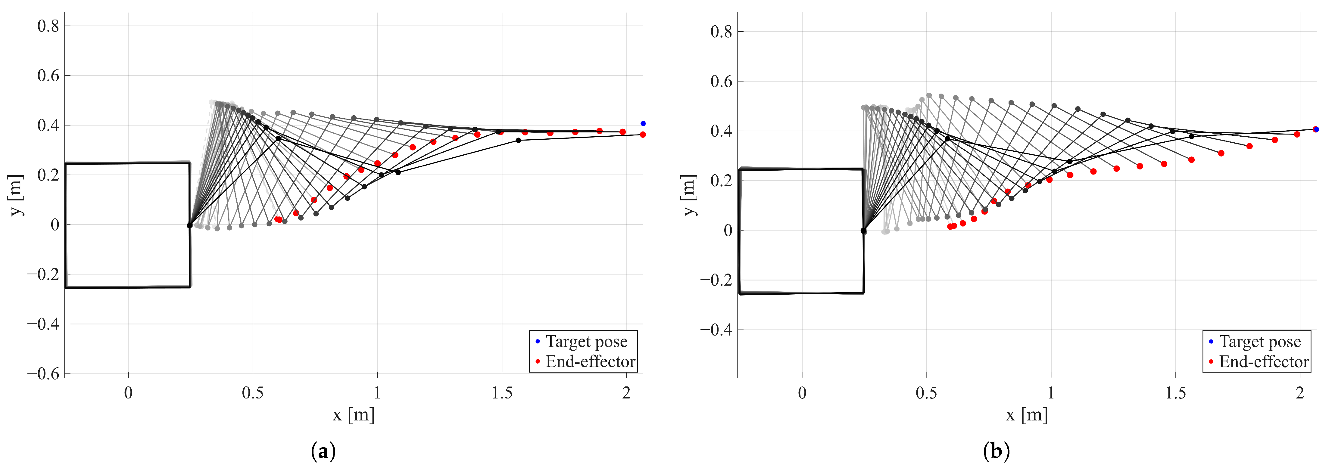
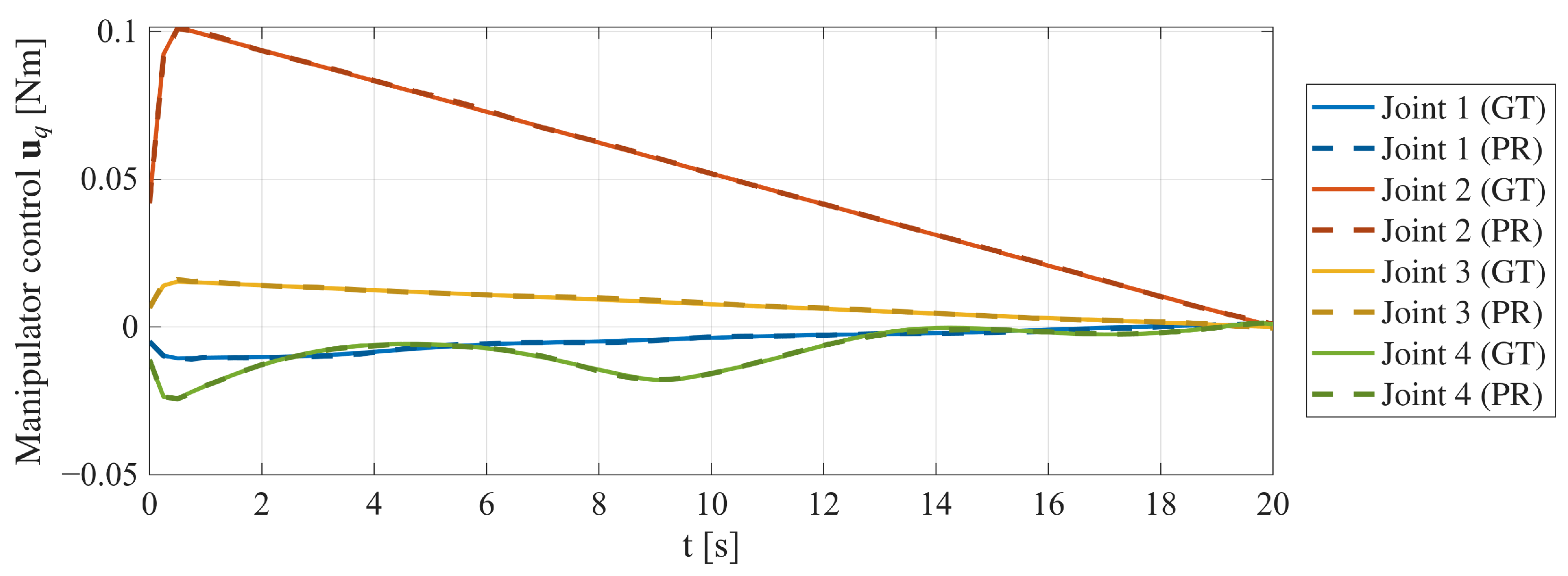
A comparison between the trajectory guess generated by the GRU network and the subsequently optimized trajectory via SCP is presented in Figure 6 for the obstacle-free dataset. Additionally, Figure 7 provides a comparison between the network-generated manipulator controls and the ground truth ones, where the similarity between the two reflects the small relative trajectory errors for the joint angle component in Table 3.

4.2. Network Conditioning and Terminal Constraint Satisfaction

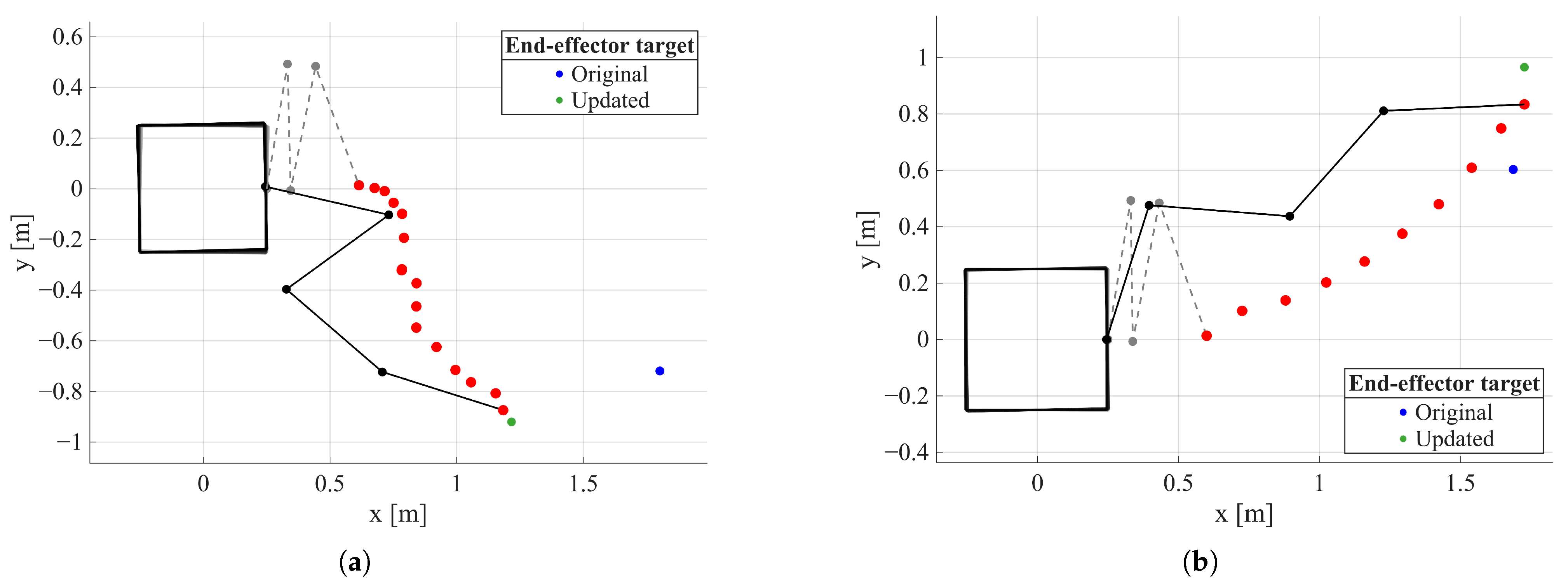
The goal of this section is to prove the effectiveness of the trajectory conditioning mechanism graphically, through a demonstrative test. The aim is to show that the vector $\mathit{g}$ actively influences the generation process, preventing the networks from simply memorizing the training dataset. To this end, at a random instant between 25–50% of the generation, the network is provided with a new end-effector pose target, requiring the trajectory to be adapted mid-generation. While this test does not yield optimal trajectory guesses due to the different nature of the problem, it verifies that the conditioning functions as expected. As seen in Figure 8, the network correctly adapts to the new goal, guiding the end-effector towards the updated target. Although visible errors in the final end-effector pose are present, these are expected since the network was not trained on this specific condition; the result remains a successful demonstration of the conditioning mechanism’s functionality.

Given the efficacy of the conditioning mechanism, an important metric to evaluate is the inferred end-effector pose error at the final timestep, relative to the target poses in the test dataset. A high-quality prediction should minimize this error to facilitate easier and faster satisfaction of the terminal constraint during optimization, further reducing the number of SCP iterations required for convergence after a warm-start. As previously mentioned, the network generates the full system state and control inputs but does not possess explicit knowledge of the end-effector pose evolution. This design allows trajectory generation to occur entirely in the joint space exploiting a task-space conditioning, eliminating the need for inverse kinematics during both the warm-start and subsequent optimization phases. The results, separated into position and attitude errors of the end-effector, are presented in

Table 5. End-effector terminal pose error between network guess and ground truth. (Values provided as Mean ± Std Dev).

Terminal Pose Error	MLP	LSTM	GRU	Transformer
Position (cm)	$4.0\pm 3.0$	$3.2\pm 2.5$	$3.3\pm 2.7$	$7.5\pm 5.7$
Attitude (deg)	$1.4\pm 1.2$	$1.1\pm 1.0$	$1.1\pm 1.0$	$2.5\pm 2.0$

. The average terminal end-effector pose errors are in the order of a few centimeters and degrees; this proximity to the target pose implies that the generated predictions are sufficiently accurate, often leaving the SCP module with only a final refinement task rather than large-scale updates to the trajectory.

Given the importance of minimizing the end-effector terminal pose error, several strategies could be explored in future works to further improve performance. First, rather than completely removing the teacher forcing phase at a fixed point during training, a small percentage of timesteps could always be inferred from the ground-truth, instead of the network’s own predictions. This partial teacher forcing throughout the whole training process would help stabilize long-horizon inference. In addition, data augmentation could be incorporated during the teacher forcing stage by injecting synthetic noise into the trajectories. This would strengthen the network’s ability to exploit the conditioning mechanism to correct its own prediction errors, particularly in the presence of trajectory drift. Finally, end-effector accuracy could be further improved by introducing an explicit terminal pose error penalty in the training loss function. This modification would naturally extend the current training framework and could be interpreted within an offline reinforcement learning context, potentially yielding additional performance gains.

4.3. SCP Iteration Improvement Through GRU Network Warm-Start

A fundamental indicator of the effectiveness of the proposed warm-starting approach is the reduction in SCP solver iterations compared to a low-quality, possibly constraint-violating initialization computed through a computed-torque controller. For this comparison, only GRU-generated guesses are considered, as this architecture emerged as the best performing in previous tests. The evaluation is conducted in both an obstacle-free environment and an environment containing a single obstacle; for the latter, the GRU was retrained using the method described in Section 3 with identical parameters, but with obstacle information appended to the conditioning vector. The quantitative results for both cases are summarized in

Table 6. GRU warm-start improvement over computed-torque cold-start (250 test trajectories).

Obstacle #	Avg. Iter. Decrease	Max Iter. Decrease
0	$8(71.7\%)$	$25(96.2\%)$
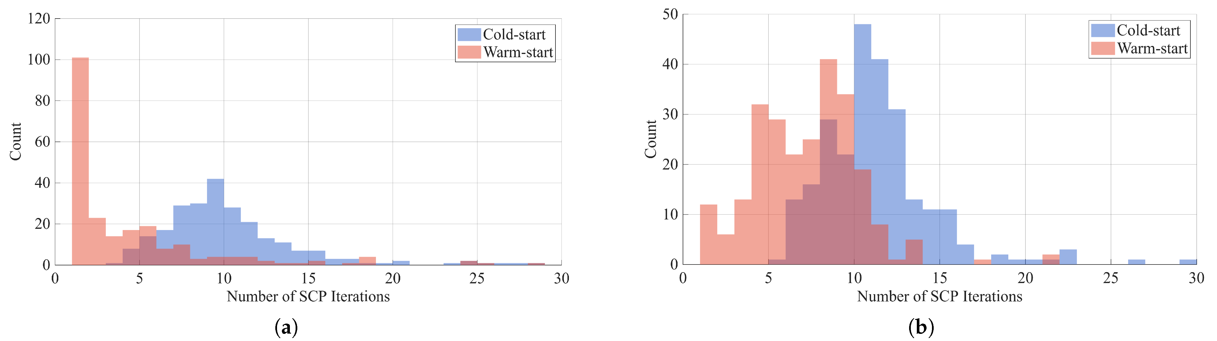
1	$5(33.5\%)$	$12(82.1\%)$

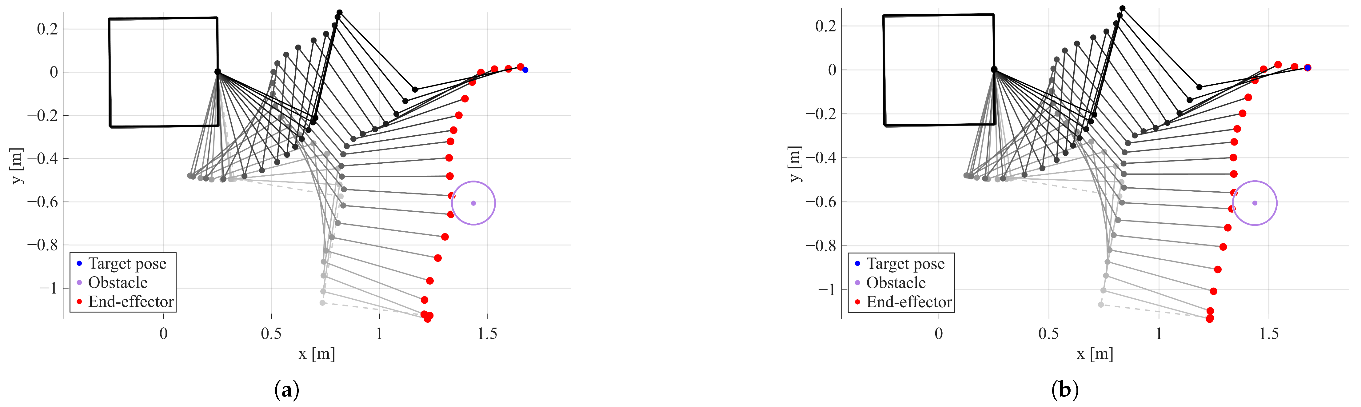
, while the respective histograms are shown in Figure 9. Warm-starting with a high-quality initial guess effectively reduces the iterations required to determine the optimal trajectory, substantially decreasing computational effort. As expected, the obstacle-free environment exhibits greater improvement due to its lower complexity, whereas the presence of obstacles requires additional iterations to guarantee collision avoidance objectives. Nonetheless, both distributions clearly shift toward lower iteration counts. Notably, when the network-generated guess is close to optimality, convergence is achieved in very few iterations; the optimizer’s role is thus to refine the predictions, ensuring dynamic feasibility and formal constraint satisfaction, as illustrated in Figure 10.

5. Conclusions

To date, the application of ML methods to spacecraft guidance and control has demonstrated enormous potential to improve performance in resource-constrained scenarios, yet it remains limited as a standalone solution due to the lack of rigorous mathematical backing for safety-critical tasks. Conversely, rigorous trajectory optimization methods often suffer from high on-board computational costs and significant sensitivity to initialization strategies. Leveraging the strengths of both approaches, this work presents a hybrid framework employing autoregressive trajectory generator networks to warm-start an SCP module for redundant space robotic systems. The networks deliver high-quality, pseudo-optimal predictions to initialize the solver, while the SCP module ensures dynamic feasibility and constraint satisfaction with formal mathematical guarantees. This integration significantly reduces the iterations needed for convergence and, consequently, the computational effort required to produce an optimal trajectory for the free-flying space robot. Notably, when high-quality guesses are generated, the role of the SCP solver is effectively reduced to a final refinement step on the predicted solution, ensuring formal constraint compliance and enabling convergence within very few iterations. Efficient solutions to such problems are poised to play a central role in future space missions, where robotic servicing agents will require fast, reliable trajectory generation methods suited to online re-planning.

Future Works

In future works, both the network prediction and SCP modules will be extended to cover a more generic set of space robot trajectory optimization problems. Incorporating physics-informed training and offline reinforcement learning strategies could significantly enhance trajectory generation quality, further improving task- and constraint-awareness of the networks; specifically, improving the dynamic feasibility of initial predictions would further simplify the downstream optimization task. While the current implementation supports any planar space robot model via URDF, extensions are planned to support generic non-planar models, thereby achieving a more flexible framework for space robot trajectory optimization. Additionally, the inclusion of time-varying obstacles and dynamic end-effector targets is foreseen, extending applicability to uncooperative and tumbling target scenarios. Having demonstrated the efficacy of the proposed OCP relaxation, the module could be adapted for compatibility with general SCP frameworks like GuSTO, providing more rigorous performance guarantees. This integration would provide access to well-established features, such as free-final-time formulations, which have already been proven across a variety of trajectory optimization tasks. Beyond simulation studies, the proposed trajectory generation methods require experimental verification. Future work will first focus on Processor-in-the-Loop and Hardware-in-the-Loop campaigns to quantify computational performance directly on space-relevant hardware. To the authors’ knowledge, autoregressive sequence models have not yet been deployed in space. While the successive inference required by these models is computationally intensive, this overhead is manageable; significantly larger neural networks are already deployed in space for on-board image processing tasks. Consequently, the initial computational cost to generate the guess is justified by the overall benefits to the optimization, as the subsequent computational effort is substantially reduced. Subsequent validation will target ground-based orbital robotics facilities, initially utilizing air-bearing testbeds like ESA’s Orbital Robotics Laboratory to assess robustness against the Sim-to-Real gap, simulating free-floating effects within a microgravity experiment. Maintaining the planar approximation in a 2D planar experiment would allow us to overcome the gravitational effects on ground, to test trajectory generation and replanning. While more representative of the planar free-floating dynamics in space, similar experiments would test the algorithm against dynamics slightly different from the modeled one, be it from the inexact model, or facility-dependent effects like small friction components or actuator dynamics with respect to the zero-order hold assumption. Once the algorithm is validated in a planar scenario, the natural extension to the 3D case could also be achieved. Utilizing robotics facilities that can recreate relative orbital dynamics motion would allow us to further strengthen the validity of the approach within a more realistic dynamic, measuring quantities like the minimum trajectory discretization needed to avoid drift and achieve end-effector tracking without violating convex approximations.

References

- LaValle, S.M. Planning Algorithms; Cambridge University Press: Cambridge, UK, 2006. [Google Scholar] [CrossRef] [Scilit]
- Mohanan, M.G.; Salgoankar, A. A survey of robotic motion planning in dynamic environments. Robot. Auton. Syst. 2018, 100, 171–185. [Google Scholar] [CrossRef] [Scilit]
- Zucker, M.; Ratliff, N.; Dragan, A.D.; Pivtoraiko, M.; Klingensmith, M.; Dellin, C.M.; Bagnell, J.A.; Srinivasa, S.S. CHOMP: Covariant Hamiltonian Optimization for Motion Planning. Int. J. Robot. Res. 2013, 32, 1164–1193. [Google Scholar] [CrossRef] [Scilit]
- Kalakrishnan, M.; Chitta, S.; Theodorou, E.; Pastor, P.; Schaal, S. STOMP: Stochastic trajectory optimization for motion planning. In Proceedings of the IEEE International Conference on Robotics and Automation, Shanghai, China, 9–13 May 2011; IEEE: New York, NY, USA, 2011; pp. 4569–4574. [Google Scholar] [CrossRef] [Scilit]
- Schulman, J.; Ho, J.; Lee, A.; Awwal, I.; Bradlow, H.; Abbeel, P. Finding Locally Optimal, Collision-Free Trajectories with Sequential Convex Optimization. In Proceedings of the Robotics: Science and Systems IX, Berlin, Germany, 24–28 June 2013. [Google Scholar] [CrossRef] [Scilit]
- Rawlings, J.B.; Mayne, D.Q.; Diehl, M.M.; Barbara, S. Model Predictive Control: Theory, Computation, and Design, 2nd ed.; Nob Hill Publishing: Santa Barbara, CA, USA, 2022. [Google Scholar]
- Pesce, V.; Colagrossi, A.; Silvestrini, S. Modern Spacecraft Guidance, Navigation, and Control; Elsevier: Amsterdam, The Netherlands, 2023. [Google Scholar] [CrossRef] [Scilit]
- Boyd, S.P.; Vandenberghe, L. Convex Optimization; Cambridge University Press: Cambridge, UK, 2004; p. 716. [Google Scholar] [CrossRef] [Scilit]
- Malyuta, D.; Reynolds, T.P.; Szmuk, M.; Lew, T.; Bonalli, R.; Pavone, M.; Acikmese, B. Convex Optimization for Trajectory Generation. IEEE Control Syst. 2022, 42, 40–113. [Google Scholar] [CrossRef] [Scilit]
- Liu, X.; Lu, P. Solving nonconvex optimal control problems by convex optimization. J. Guid. Control Dyn. 2014, 37, 750–765. [Google Scholar] [CrossRef] [Scilit]
- Mao, Y.; Szmuk, M.; Açıkmeşe, B.A. Successive Convexification of Non-Convex Optimal Control Problems and Its Convergence Properties. In Proceedings of the 2016 IEEE 55th Conference on Decision and Control (CDC), Las Vegas, NV, USA, 12–14 December 2016; IEEE: New York, NY, USA, 2016. [Google Scholar] [CrossRef] [Scilit]
- Misra, G.; Bai, X. Optimal path planning for free-flying space manipulators via sequential convex programming. J. Guid. Control Dyn. 2017, 40, 3019–3026. [Google Scholar] [CrossRef] [Scilit]
- Virgili-Llop, J.; Zagaris, C.; Zappulla, R.; Bradstreet, A.; Romano, M. A convex-programming-based guidance algorithm to capture a tumbling object on orbit using a spacecraft equipped with a robotic manipulator. Int. J. Robot. Res. 2019, 38, 40–72. [Google Scholar] [CrossRef] [Scilit]
- Sutton, R.S.; Barto, A.G. Reinforcement Learning: An Introduction; Westchester Publishing Services: Danbury, CT, USA, 2018; p. 526. [Google Scholar] [CrossRef] [Scilit]
- Ali, A.A.; Shi, J.F.; Zhu, Z.H. Path planning of 6-DOF free-floating space robotic manipulators using reinforcement learning. Acta Astronaut. 2024, 224, 367–378. [Google Scholar] [CrossRef] [Scilit]
- D’Ambrosio, M.; Capra, L.; Brandonisio, A.; Silvestrini, S.; Lavagna, M. Redundant Space Manipulator Autonomous Guidance for In-Orbit Servicing via Deep Reinforcement Learning. Aerospace 2024, 11, 341. [Google Scholar] [CrossRef] [Scilit]
- D’Ambrosio, M.; Lavagna, M. Enhancing Space Manipulator Fault Tolerance for In-Orbit Servicing through Meta-Reinforcement Learning. In Proceedings of the CEAS Conference 2025, Turin, Italy, 1–4 December 2025. [Google Scholar]
- Janner, M.; Li, Q.; Levine, S. Offline Reinforcement Learning as One Big Sequence Modeling Problem. arXiv 2021, arXiv:2106.02039. [Google Scholar] [CrossRef] [Scilit]
- Chen, L.; Lu, K.; Rajeswaran, A.; Lee, K.; Grover, A.; Laskin, M.; Abbeel, P.; Srinivas, A.; Mordatch, I. Decision Transformer: Reinforcement Learning via Sequence Modeling. arXiv 2021, arXiv:2106.01345. [Google Scholar] [CrossRef] [Scilit]
- Silvestrini, S.; Lavagna, M. Deep Learning and Artificial Neural Networks for Spacecraft Dynamics, Navigation and Control. Drones 2022, 6, 270. [Google Scholar] [CrossRef] [Scilit]
- Guffanti, T.; Gammelli, D.; D’Amico, S.; Pavone, M. Transformers for Trajectory Optimization with Application to Spacecraft Rendezvous. In Proceedings of the 2024 IEEE Aerospace Conference, Big Sky, MT, USA, 2–9 March 2024; IEEE: New York, NY, USA, 2024. [Google Scholar] [CrossRef] [Scilit]
- Banerjee, S.; Lew, T.; Bonalli, R.; Alfaadhel, A.; Alomar, I.A.; Shageer, H.M.; Pavone, M. Learning-based Warm-Starting for Fast Sequential Convex Programming and Trajectory Optimization. In Proceedings of the 2020 IEEE Aerospace Conference, Big Sky, MT, USA, 7–14 March 2020; IEEE: New York, NY, USA, 2020. [Google Scholar] [CrossRef] [Scilit]
- Bonalli, R.; Cauligi, A.; Bylard, A.; Pavone, M. GuSTO: Guaranteed Sequential Trajectory Optimization via Sequential Convex Programming. In Proceedings of the 2019 International Conference on Robotics and Automation (ICRA), Montreal, QC, Canada, 20–24 May 2019; IEEE: New York, NY, USA, 2019. [Google Scholar] [CrossRef] [Scilit]
- Celestini, D.; Gammelli, D.; Guffanti, T.; D’Amico, S.; Capello, E.; Pavone, M. Transformer-based Model Predictive Control: Trajectory Optimization via Sequence Modeling. IEEE Robot. Autom. Lett. 2024, 9, 9820–9827. [Google Scholar] [CrossRef] [Scilit]
- Gurobi Optimization, LLC. Gurobi Optimizer Reference Manual. 2024. Available online: https://www.gurobi.com (accessed on 1 May 2025).
- Tedrake, R. Underactuated Robotics. 2023. Available online: https://underactuated.csail.mit.edu (accessed on 20 July 2025).
- Andersson, J.A.; Gillis, J.; Horn, G.; Rawlings, J.B.; Diehl, M. CasADi: A software framework for nonlinear optimization and optimal control. Math. Program. Comput. 2019, 11, 1–36. [Google Scholar] [CrossRef] [Scilit]
- Virgili-Llop, J.; Drew, J.V., II; Romano, M. SPART SPAcecraft Robotics Toolkit: An Open-Source Simulator for Spacecraft Robotic Arm Dynamic Modeling And Control. In Proceedings of the 6th International Conference on Astrodynamics Tools and Techniques, Spacecraft Robotics Laboratory, Naval Postgraduate School, Darmstadt, Germany, 14–17 March 2016. [Google Scholar]
- Siciliano, B.; Oussama, K. Springer Handbook of Robotics; Springer: Berlin/Heidelberg, Germany, 2008; pp. 1031–1063. [Google Scholar] [CrossRef] [Scilit]
- Morgan, D.; Chung, S.J.; Hadaegh, F.Y. Model predictive control of swarms of spacecraft using sequential convex programming. J. Guid. Control Dyn. 2014, 37, 1725–1740. [Google Scholar] [CrossRef] [Scilit]
- Liu, X.; Li, Y.; Jiang, H.; Song, T. Exact Convex Relaxation Using Supporting Hyperplane for Trajectory Optimization of UAVs. J. Guid. Control Dyn. 2025, 48, 2512–2526. [Google Scholar] [CrossRef] [Scilit]
- Lew, T.; Bonalli, R.; Pavone, M. Chance-Constrained Sequential Convex Programming for Robust Trajectory Optimization. In Proceedings of the European Control Conference, St. Petersburg, Russia, 12–15 May 2020. [Google Scholar] [CrossRef] [Scilit]
- Mao, Y.; Szmuk, M.; Xu, X.; Acikmese, B. Successive Convexification: A Superlinearly Convergent Algorithm for Non-convex Optimal Control Problems. arXiv 2019, arXiv:1804.06539. [Google Scholar] [CrossRef] [Scilit]
- CVX Research, Inc. CVX: Matlab Software for Disciplined Convex Programming, Version 2.0. 2012. Available online: https://cvxr.com/cvx (accessed on 1 May 2024).
- Goodfellow, I.; Bengio, Y.; Courville, A. Deep Learning; MIT Press: Cambridge, MA, USA, 2016. [Google Scholar]
- Salinas, D.; Flunkert, V.; Gasthaus, J.; Januschowski, T. DeepAR: Probabilistic forecasting with autoregressive recurrent networks. Int. J. Forecast. 2020, 36, 1181–1191. [Google Scholar] [CrossRef] [Scilit]
- Triebe, O.; Laptev, N.; Rajagopal, R. AR-Net: A simple Auto-Regressive Neural Network for time-series. arXiv 2019, arXiv:1911.12436. [Google Scholar] [CrossRef] [Scilit]
Figure 1.
Hybrid trajectory optimization framework.
Figure 2.
Affine approximation of collision avoidance constraint.
Figure 3.
Representation of planar space robot trajectory evolution over time, maneuvering the manipulator from the initial configuration to achieve the final end-effector target pose: (a) Low-quality initial guess trajectory. (b) Optimized space robot trajectory.
Figure 4.
Autoregressive trajectory generation loop: (a) Models with non-recurrent core using k-step buffer (MLP, Transformer). (b) Models with recurrent core (LSTM, GRU).
Figure 5.
Network inference mode shown through unrolled autoregressive loop (Ground truth , Network inference ): (a) Teacher forcing mode. (b) Nominal autoregressive mode.
Figure 6.
(a) GRU-generated trajectory guess. (b) Trajectory after warm-started SCP optimization.
Figure 7.
Example GRU prediction (PR) vs. ground truth (GT): manipulator control torques.
Figure 8.
Demonstration of conditioning mechanism effectiveness (first and last timesteps only, with end-effector evolution in red). (a) Example 1. (b) Example 2.
Figure 9.
SCP iteration comparison: (a) Obstacle-free scenario. (b) Single-obstacle scenario.
Figure 10.
Trajectory example with obstacle: (a) GRU-generated guess. (b) Optimized trajectory.