Dynamics Modeling of a Rigid–Flexible Coupled Flapping-Wing Robot and Diffeomorphism-Based Disturbance Rejection Attitude-Constrained Control

Abstract

Lightweight flapping-wing robots are affected by structural flexibility, wind disturbances, and static friction in basal passive joints during perching and attitude-holding tasks. These coupled effects can make conventional PID and sliding mode control (SMC) produce error amplification, torque fluctuation, flexible-response excitation, and attitude-boundary violation. This study establishes an ADAMS–Simulink co-simulation platform for a rigid–flexible coupled flapping-wing robot and proposes a diffeomorphism-based attitude-constrained controller. The inverse hyperbolic tangent mapping transforms bounded physical errors into unbounded virtual errors, allowing smooth small-error regulation and stronger constraint enforcement near safety boundaries. Wind-free tracking, compound wind rejection, pulse wind scanning, mapping-parameter sensitivity, and a CBF-QP safety-filtered baseline are evaluated. In manuscript parameter-synchronized ADAMS 2024 reruns under a 2 m/s steady wind with a 1 m/s pulse, PID and SMC show runaway angular excursions of 1602.56° and 381,330.03°, whereas the proposed method remains bounded at 23.58° with an RMSE of 2.943° and no boundary violation. The CBF-QP baseline still violates the boundary at 1394°. The results show improved tracking accuracy, boundary protection, measured-channel flexible-excitation attenuation, and stable disturbance recovery.

1. Introduction

In recent years, flapping-wing aerial robots have shown considerable application potential in post-disaster exploration, industrial inspection, and ecological monitoring owing to their efficient aerodynamic characteristics and bio-inspired locomotion mechanisms. To extend their mission duration and overcome the limitations imposed by battery endurance, increasing attention has been paid to enabling flapping-wing robots with bird-like perching and grasping capabilities, which has become an active research topic in robotics [1,2,3,4]. In nature, birds can perch stably on branches by exploiting the static friction generated by their claws. After folding their wings, they can further interact with targets through body balancing and beak-assisted manipulation. When this biological mechanism is transferred to robotic systems, the perching system can be modeled as an underactuated multi-link manipulator with passive joints that represent the static-friction effect of avian claws [5,6,7,8,9,10,11]. However, because the output torque of lightweight aerial micro-motors is limited and the anti-overturning capability at the base of the system relies mainly on static friction, preventing slip-induced failure during large-angle motion remains a challenging attitude-constrained control problem.

Several studies have investigated underactuated systems with passive friction joints. For example, diffeomorphism-based mappings and control barrier functions have been employed to address trajectory-tracking problems with state constraints under idealized conditions [12,13]. Nevertheless, most existing studies are based on simplified assumptions and usually neglect the effects of structural flexibility and complex aerodynamic disturbances. In practical applications, the supporting limbs of robots, such as links mimicking avian legs, are often designed as slender structures, making them prone to significant elastic deformation during large-angle motion [14,15,16]. Unmodeled flexible dynamics may couple with conventional unconstrained controllers, such as PID controllers, leading to actuator saturation, flexible-mode excitation, or resonance in multibody structures. Moreover, outdoor environments are frequently accompanied by complex wind disturbances. Owing to their lack of boundary-awareness, conventional linear control strategies are generally unable to attenuate measured flexible-excitation effects effectively or respond in time to the critical condition of static-friction failure, which may eventually result in system instability.

To reduce the gap between theoretical modeling and practical operating conditions, this study introduces a diffeomorphism-based nonlinear attitude control strategy on the basis of rigid-body dynamic modeling. Furthermore, a multibody dynamics co-simulation platform incorporating structural flexibility and compound aerodynamic disturbances is developed to analyze the disturbance-rejection mechanism and robustness of the proposed control strategy under complex operating conditions. The main contributions of this study are summarized as follows:

• C1. A cross-domain co-simulation platform incorporating flexible links and compound wind disturbances is established. By integrating ADAMS and Simulink, the proposed platform overcomes the limitations of single-software simulation and enables the coupled analysis of large-deformation flexible links and compound gust disturbances, including a 2 m/s baseline wind, a 1 m/s transient pulse disturbance, and white noise.
• C2. The nonlinear regulation mechanism of diffeomorphic mapping for attenuating measured-channel flexible excitation is investigated. The results verify that the proposed method can reduce the influence of high-frequency components in the measured feedback and torque-response channels and improve the dynamic stability of the system.
• C3. It is demonstrated that, under transient pulse wind disturbances, the diffeomorphism-based nonlinear control strategy can prevent boundary loss through boundary-aware error reshaping. After the disturbance disappears, the proposed method enables stable attitude recovery, thereby achieving robust stabilization and pose restoration in transient gust environments.

Through these contributions, this study provides theoretical support and engineering reference for reliable perching and operation of flapping-wing robots under complex meteorological conditions.

2. Materials and Methods

This section defines the rigid–flexible multibody model, compound wind disturbance, attitude-constrained controller, and ADAMS–Simulink implementation used to evaluate tracking, disturbance rejection, measured-channel flexible-excitation attenuation, and boundary protection.

2.1. System Dynamics and Environmental Modeling

Real perching occurs under gusts and structural compliance, whereas many underactuated bio-inspired manipulator models assume rigid bodies and simplified environments [17,18]. The present model therefore uses ADAMS–Simulink co-simulation to represent a flexible multibody mechanism under wind disturbances [19,20].

2.1.1. Baseline Rigid-Body Configuration and Nominal Trajectory Definition

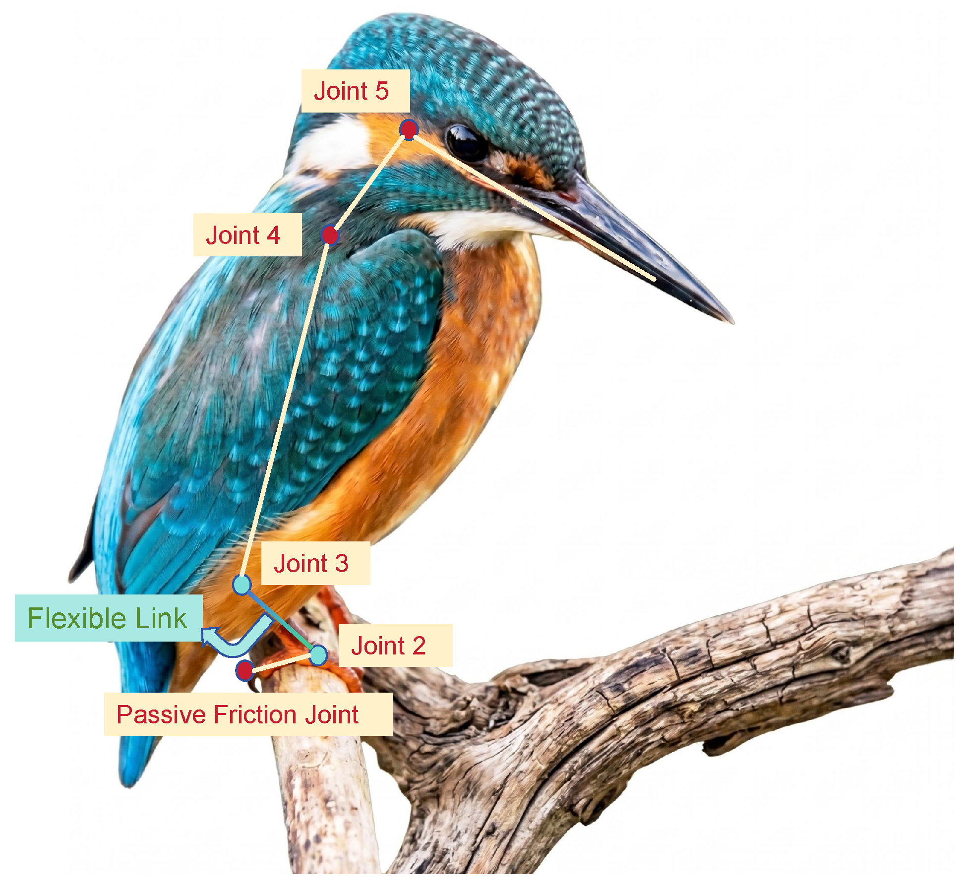
Referring to the anatomical characteristics of avian lower limbs [9,17], the basic structure of the proposed system is defined as a multi-link underactuated mechanism and simplified as five interconnected links, as shown in Figure 1. The first joint, which connects the bottom link to the perching surface, serves as the grasping support point of the claw. This joint is designed as a motor-free passive joint and relies entirely on static friction to maintain the balance of the system.

To clarify the physical parameters of the co-simulation model and improve its reproducibility, the main structural parameters, inertial parameters, and joint constraint parameters of the five links in the ADAMS 2024 rerun model are summarized in

Table 1. Main structural and constraint parameters of the rigid–flexible coupled system.

(a) Structural and inertial parameters
Link No.	ADAMS Part	Physical Meaning	$\mathit{L}$/mm	$\mathit{m}$/kg	$({\mathit{x}}_{\mathit{c}},{\mathit{y}}_{\mathit{c}},{\mathit{z}}_{\mathit{c}})$/mm	$({\mathit{I}}_{\mathit{xx}},{\mathit{I}}_{\mathit{yy}},{\mathit{I}}_{\mathit{zz}})$/kg·mm2
1	PART_2	Bottom support and perching-contact segment	30	0.0091609	$(0,15,0)$	$(0.8726,0.8726,0.3710)$
2	PART_3_flex	Flexible bio-inspired leg link	120	0.0286896	$(0,90,-1.38\times {10}^{-7})$	$(267.2359,0.7643,267.2360)$
3	PART_4	Intermediate attitude-regulation link	150	0.0747856	$(0,225,0)$	$(142.6956,142.6956,4.9452)$
4	PART_5	Upper attitude-regulation link	60	0.0299142	$(0,330,0)$	$(9.9633,9.9633,1.9781)$
5	PART_6	Distal attitude-regulation link	50	0.0092363	$(0,385,0)$	$(2.0374,2.0374,0.2263)$
(b) Joint and actuation/constraint parameters
Link No.	ADAMS Part	Joint Type	Actuation/Constraint Parameters
1	PART_2	Passive revolute joint; passive friction joint	FRICTION_1; ${\mu }_s=0.3$, ${\mu }_d=0.2$; friction arm: 1.0 mm; pin radius: 9.0 mm; friction preload torque: 150 N·mm.
2	PART_3_flex	Active revolute joint; JOINT_2	SFORCE_1; torque input: CTRL_T2.
3	PART_4	Active revolute joint; JOINT_3	SFORCE_1_2; torque input: CTRL_T3.
4	PART_5	Active revolute joint; JOINT_4	SFORCE_1_3; torque input: CTRL_T4.
5	PART_6	Active revolute joint; JOINT_5	SFORCE_1_4; torque input: CTRL_T5.

Note: “No explicit torque saturation limit” refers only to the ADAMS-side SFORCE actuator elements listed in Table 1. These elements are used as rotational torque interfaces, whereas the controller-side output constraints are implemented in Simulink and are described in the controller implementation section.

. The model adopts the MMKS unit system, in which the length, mass, force, time, and angular units are mm, kg, N, s, and deg, respectively. Therefore, the controller-command torques, measured joint torque responses, equivalent aerodynamic disturbance torques, and joint constraint torques in this study are uniformly expressed in N·mm. The five links correspond to PART_2, PART_3_flex, PART_4, PART_5, and PART_6 in the ADAMS model. Among them, PART_3_flex is the flexible link used to mimic the avian leg; it is imported through an MNF file and defined as a flexible body, whereas the remaining links are modeled as rigid bodies.

The parameters in Table 1 are taken from the ADAMS configuration. Link 2 is the MNF-based flexible body PART_3_flex, while the other links remain rigid. Simulink generates controller-command torques for joints 2–5, ADAMS applies them through SFORCE interfaces, and measured joint torque responses are extracted from ADAMS output channels. The basal JOINT_1 is an unactuated passive revolute joint with FRICTION_1 and an equivalent static-friction preload torque of 150 N·mm.

The nominal perching attitude sets the active-joint targets to ${40}^{\circ }$, $-{20}^{\circ }$, ${15}^{\circ }$, and $0^{\circ }$ for joints 2–5, respectively. This step task is used as the baseline for later controller comparisons.

2.1.2. Rigid–Flexible Coupled Dynamic Model of the Bio-Inspired Leg Link

Link 2 mimics a slender avian leg and is therefore modeled as the main compliant load-bearing component. During large-angle or abrupt motion, its deformation can excite high-frequency whip-like oscillations that conventional rigid-body PID feedback may misinterpret as tracking error, amplifying noise and destabilizing the loop.

Link 2 is reconstructed in ADAMS using the modal neutral file (MNF) method. As the component between the basal passive joint and the upper active joint, it bears bending loads and transmits dynamic impacts from step inputs, torque variations, and pulse wind disturbances. Treating this link as flexible allows the model to capture its influence on joint feedback, controller-command torque generation, measured joint torque response, and stability [21].

The flexible link uses the CFRP_Fiber material defined in ADAMS and is modeled as an isotropic material. Its main material parameters are assigned according to the ADAMS material settings and the typical property ranges of CFRP/FRP materials [22,23]:

$$\begin{array}{cc}\hfill \rho & =1.6\times {10}^{-6}\mathrm{kg}/{\mathrm{mm}}^3,\hfill \\ \hfill E& =7.0\times {10}^4\mathrm{N}/{\mathrm{mm}}^2,\hfill \\ \hfill \nu & =0.30,\hfill \end{array}$$

(1)

where $\rho$ denotes the material density, E is Young’s modulus, and $\nu$ is Poisson’s ratio.

These values represent a lightweight composite link with low density and high specific stiffness.

During flexible-body generation, the geometric model of link 2 is first discretized in the ADAMS/Flex environment, and attachment points are defined at the two joint-connection locations to ensure the kinematic constraint relationship between the flexible body and adjacent rigid links. Subsequently, the modal synthesis method is used to generate the modal neutral file [24], which is re-imported into the ADAMS multibody system to form the flexible body PART_3_flex. The MNF file used in this study is PART_3_0.mnf. The flexible body contains 1108 nodes and 24 modes in total. In the simulation, the 7th to 24th elastic modes are retained for calculation, whereas the first six modes mainly correspond to the overall rigid-body motion of the flexible body and are therefore not included as independent elastic modes for flexible-response interpretation.

Table 2. Representative elastic modal parameters of the flexible link PART_3_flex.

Mode Order	Circular Frequency $\mathit{\omega }$/rad·s−1	Natural Frequency f/Hz
7	5868.66	933.55
8	5882.65	936.25
9	15,220.68	2422.45
10	15,270.15	2430.32
11	19,838.21	3157.35
12	31,855.43	5069.95

lists representative elastic modal parameters of PART_3_flex. Although the low-order elastic modes are high frequency, step inputs, pulse wind, and rapid torque variation can still excite them and feed their effects into joint-angle feedback. This modal response is a key source of PID error amplification and measured torque-response oscillation.

The PART_3_flex damping coefficients are kept at their default values, with no additional damping file, damping function, or generalized damping option. Thus, the flexible response is mainly determined by the modal mass, modal stiffness, and retained 7th–24th elastic modes.

2.1.3. Modeling of Transient Pulse Compound Crosswind Disturbances

External airflow is included because perching or grasping near open edges can be destabilized by lateral gusts. In Simulink, the compound wind field is represented by a steady baseline, a transient pulse, and band-limited white noise [25]:

$$v_{\mathrm{wind}}\left(t\right)=v_{\mathrm{const}}+v_{\mathrm{pulse}}\left(t\right)+v_{\mathrm{noise}}\left(t\right).$$

(2)

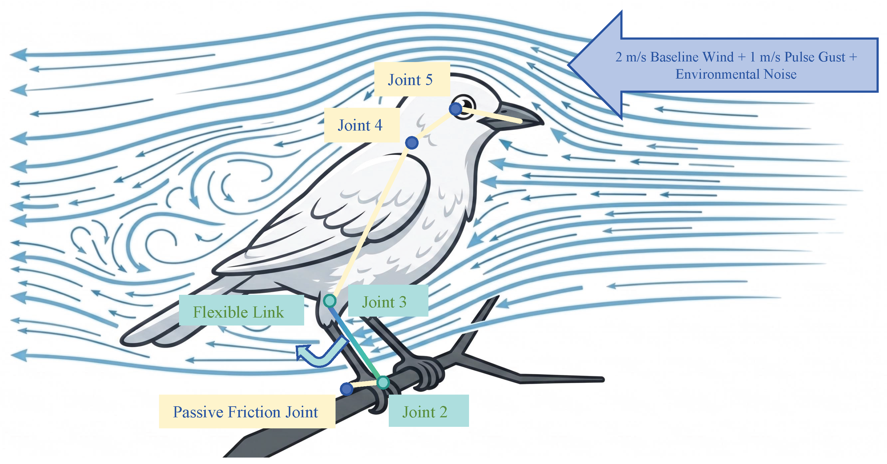
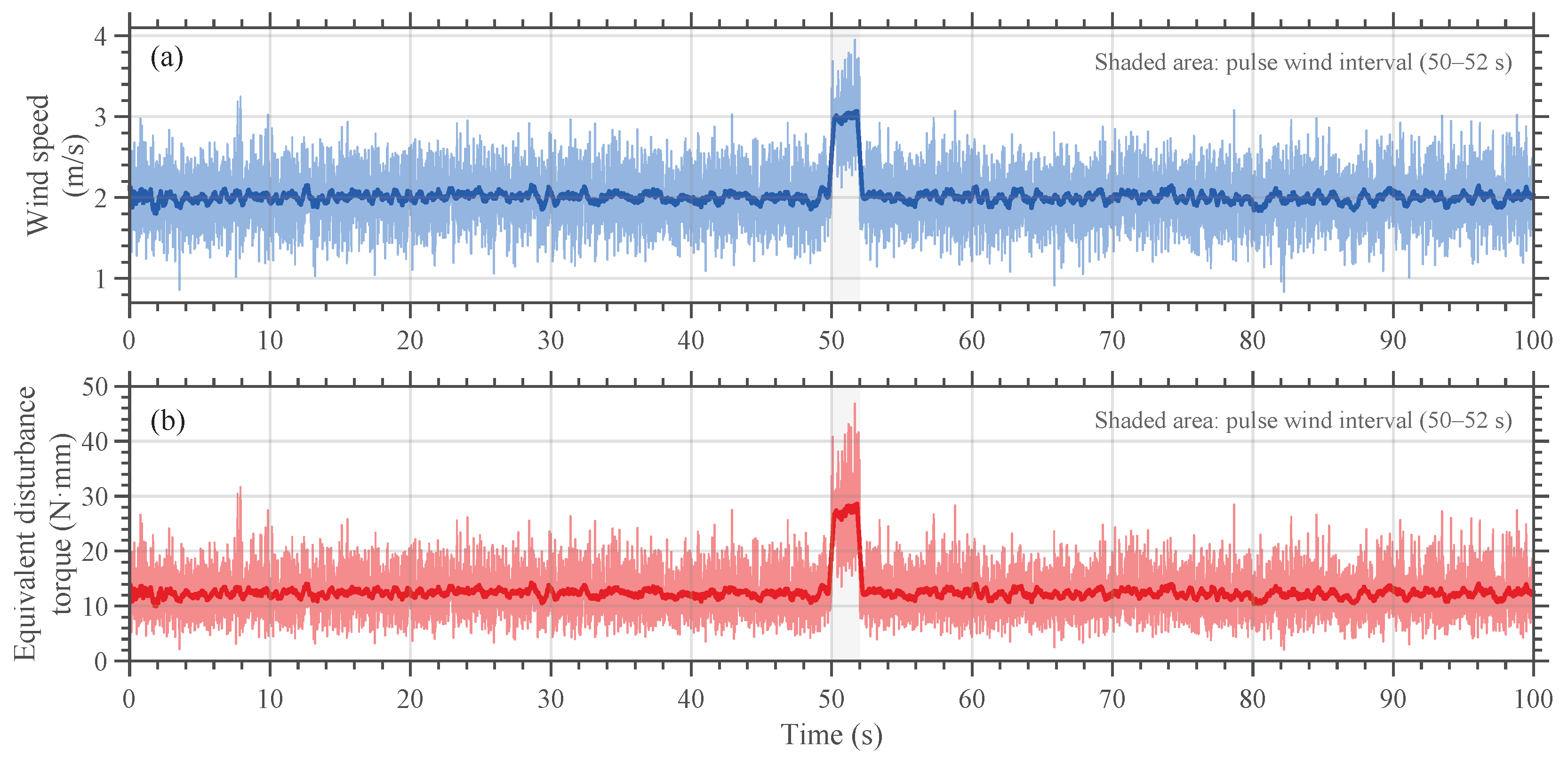
The baseline wind is $v_{\mathrm{const}}=2$ m/s. Band-limited white noise is added with a noise power of 0.1 and a sampling time of 0.01 s. A 1 m/s pulse gust is triggered at 50 s and lasts until 52 s, raising the instantaneous compound wind speed to approximately 3 m/s, as shown in Figure 2.

According to the empirical aerodynamic torque formula

$$M={\displaystyle \frac{1}{2}}\rho v^2{C}_{M}SL$$

(3)

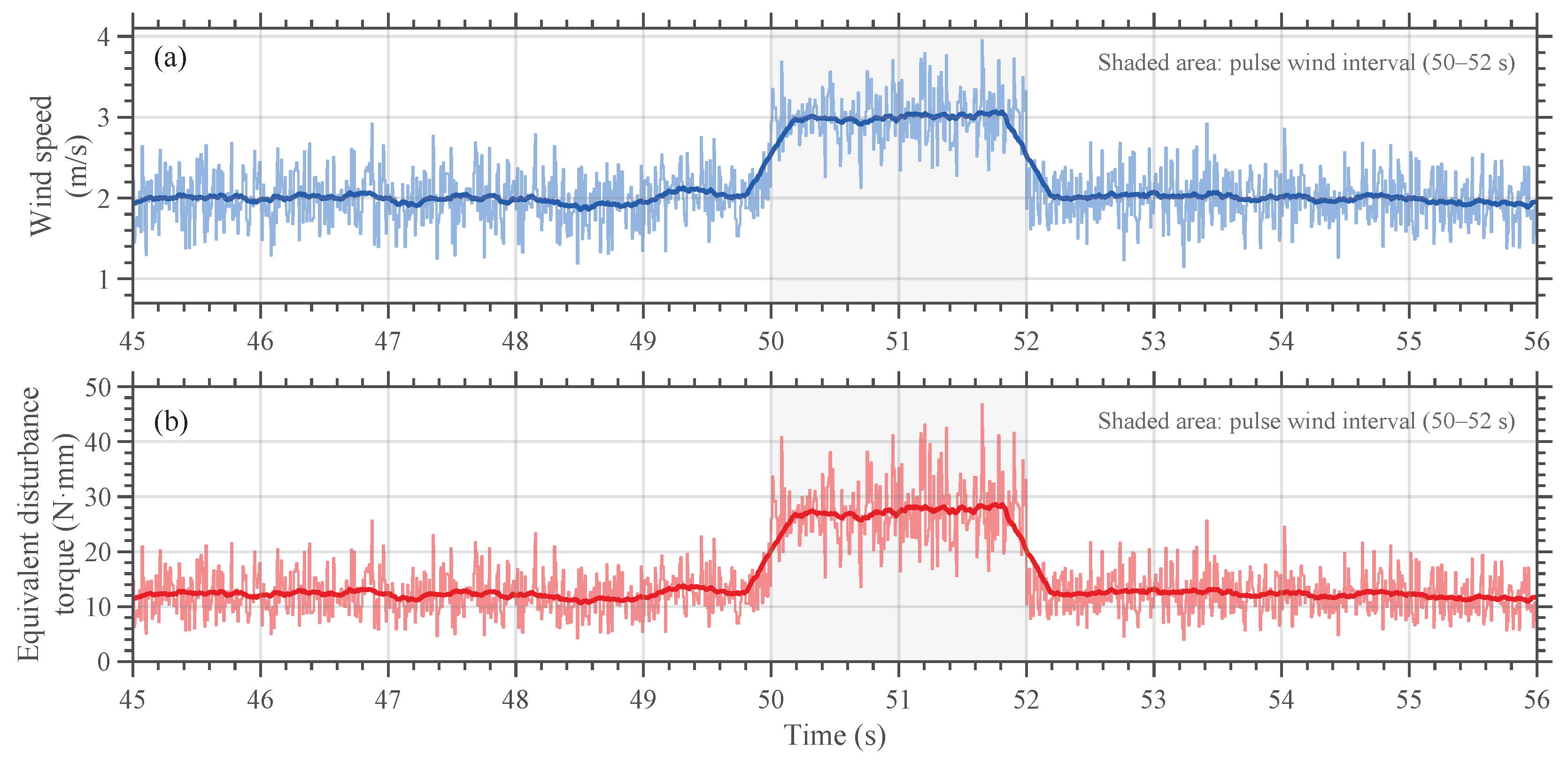
where $\rho$ is air density, $C_M$ is the moment coefficient, S is the reference windward area, and L is the characteristic length. Because $M\propto v^2$, increasing wind speed from 2.00 to 3.00 m/s raises the theoretical load by about 2.25 times. In Figure 3 and Figure 4, the equivalent disturbance torque increases from approximately 12.37 to 27.35 N·mm, with a pulse peak of 46.82 N·mm.

The full and enlarged time histories in Figure 3 and Figure 4 confirm the steady background wind, the abrupt 50–52 s pulse interval, and the synchronized increase in equivalent disturbance torque.

2.2. Problem Formulation and Control Strategy

The control objective is to maintain basal passive-joint safety while the upper multi-joint body tracks its target under flexible dynamics and pulse wind. A diffeomorphic mapping is used to transform constrained errors into an unconstrained space [12,13], consistent with the safety-set concept in constrained control and control barrier functions [26].

2.2.1. Static-Friction Failure Risk in Perching and Grasping

The first joint is an underactuated passive joint without motor actuation or rigid fixation. Its balance depends on the static-friction torque ${\tau }_c$.

During trajectory tracking, pulse gusts and flexible link whip-like vibration can increase the torque transmitted to the basal passive joint. Stability requires

$$|{\tau }_1|\le {\tau }_{c,l}.$$

(4)

To introduce an additional safety margin, a conservative attitude error safety set is defined as

$${\Omega }_a=[-a,a],$$

(5)

where a is the conservative attitude error safety boundary in deg. It is not a direct conversion of the static-friction torque limit ${\tau }_{c,l}$; rather, it represents a safety margin against center-of-mass shift, flexible link inertia, active-joint coupling, and wind disturbance. The nominal value is $a={45}^{\circ }$, and $a={35}^{\circ }$, ${45}^{\circ }$, and ${55}^{\circ }$ are later compared to evaluate the trade-off between boundary strength, recovery, measured torque response, and boundary violation.

Conventional PID control is boundary-blind: when the error approaches a, it increases output without recognizing that the passive-joint grip is approaching failure.

2.2.2. Physical Mechanism of the Diffeomorphism-Based “Nonlinear Air Wall” for Boundary-Aware Flexible-Excitation Attenuation

To make the controller boundary-aware, this study applies diffeomorphic mapping to the rigid–flexible coupled plant rather than to an ideal rigid-body model alone.

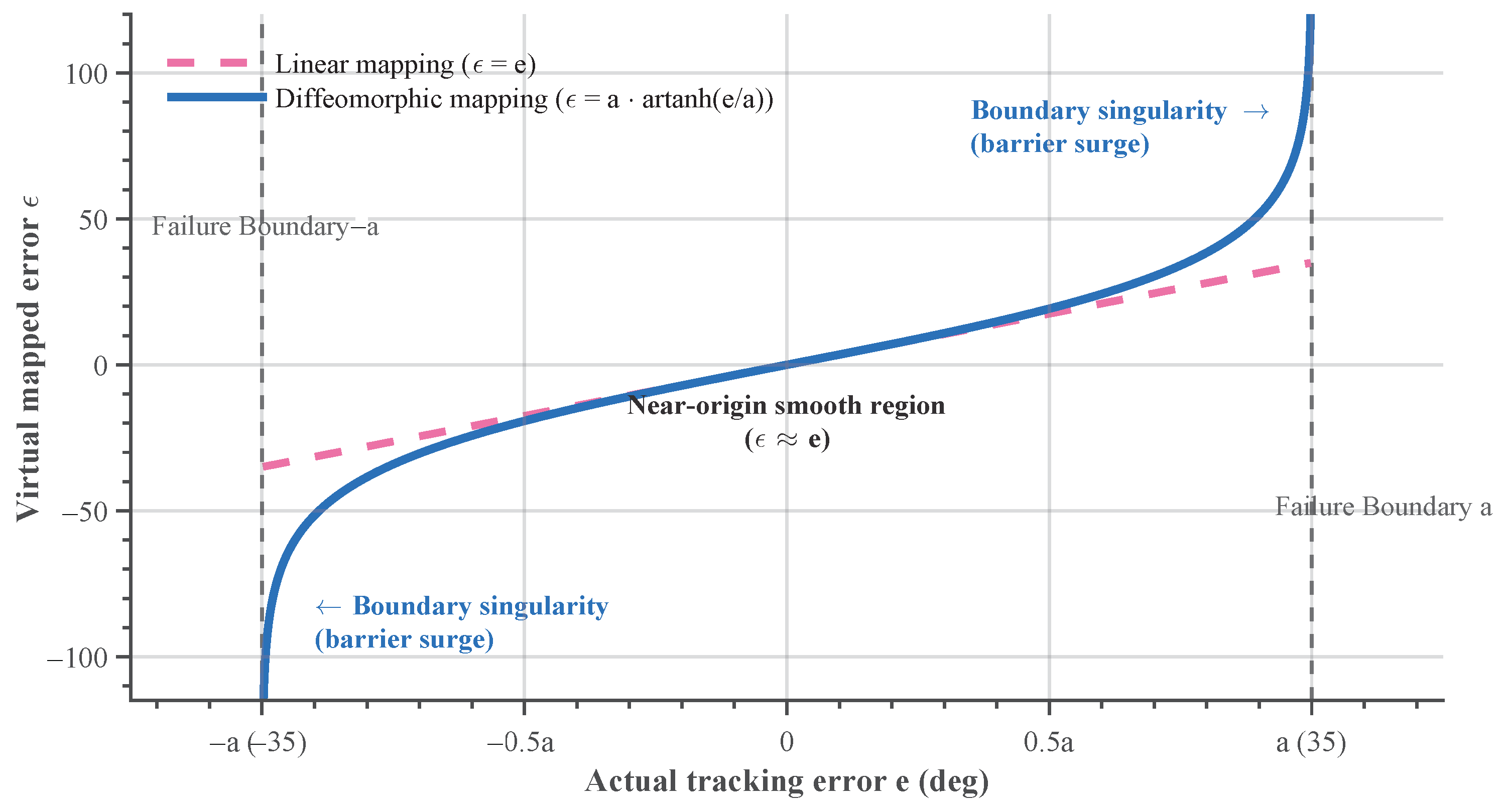
Assume that the actual tracking error of the system is e, and the safety boundary associated with the static-friction margin is a. In the control loop, an inverse hyperbolic tangent mapping is introduced to transform the physical error e into the virtual error $\epsilon$:

$$\epsilon =a\mathrm{arctanh}\left({\displaystyle \frac{e}{a}}\right),\left|e\right|<a.$$

(6)

This diffeomorphic transformation maps the finite physical-error interval into an unbounded virtual-error space [12,13]. As shown in Figure 5, it acts as a nonlinear air wall near the prescribed boundary.

Near steady state, small high-frequency fluctuations from link 2 produce small variations in e, and the mapping is approximately linear, $\epsilon \approx e$. This local smoothness prevents excessive controller response to measured flexible noise.

Under severe conditions such as a 3 m/s pulse crosswind, $|e/a|\to 1$ causes $\epsilon$ to increase rapidly. The controller therefore strengthens reverse compensation near the boundary, helping maintain stability and accelerate recovery after transient gusts.

2.2.3. Controller Implementation and Co-Simulation Input Form

To ensure comparability among different control methods, a unified joint attitude error definition is adopted for the PID, SMC, and diffeomorphism-based controllers. Let $q_{d,i}$ denote the desired angle of the ith active joint, and let $q_i$ denote the actual joint angle fed back from ADAMS. The joint attitude error is defined as

$$e_i=q_{d,i}-q_i,i=2,3,4,5.$$

(7)

Here, $e_i$ is expressed in deg. The error vector of the four active joints is written as

$$\mathbf{e}={[e_2,e_3,e_4,e_5]}^T.$$

(8)

For the PID and SMC controllers, the controller-command torque is directly calculated from the physical error $e_i$. By contrast, for the diffeomorphism-based controller, the constrained physical error $e_i$ is first mapped into the unbounded virtual error ${\epsilon }_i$, which is then used as the input of the subsequent PID-type feedback loop. The mapping relation is

$${\epsilon }_i=a\mathrm{arctanh}\left({\displaystyle \frac{e_i}{a}}\right),\left|e_i\right|<a.$$

(9)

For small $|e_i|$, ${\epsilon }_i$ is nearly linear and the controller remains smooth. As $|e_i|$ approaches a, the nonlinear gain of $\mathrm{arctanh}(·)$ increases, providing boundary-aware error reshaping without changing the physical joint angle.

Torque signals are distinguished at two levels. ADAMS SFORCE elements act only as rotational torque interfaces and do not impose independent hardware-like saturation. Simulink computes the controller-command torque, where PID uses output saturation, SMC is bounded by $\tanh (·)$ and $K_i$, and the proposed controller uses mapped-error PID-type feedback. By contrast, the measured joint torque response is extracted from ADAMS output channels and reflects the coupled plant response under controller action, rigid–flexible coupling, passive-joint friction, constraint reactions, and disturbances.

The PID controller is implemented using the continuous-time PID Controller block in Simulink. Its control law is expressed as

$${\tau }_i^{\mathrm{PID}}=K_{p,i}{e}_i+K_{i,i}\int e_{i}dt+K_{d,i}{\displaystyle \frac{N_{i}s}{s+N_i}}{e}_i,$$

(10)

where $K_{p,i}$, $K_{i,i}$, and $K_{d,i}$ are the PID gains, and $N_i$ is the derivative-filter coefficient. The parameter signs follow the ADAMS–Simulink interface convention and are listed in

Table 3. PID controller parameters.

Control Channel	ADAMS Input	Active Joint	${\mathit{K}}_{\mathit{p}}$	${\mathit{K}}_{\mathit{i}}$	${\mathit{K}}_{\mathit{d}}$	Filter Coefficient N
PID Controller 1	CTRL_T2	Joint 2	−2	−0.05	−0.05	10
PID Controller 2	CTRL_T3	Joint 3	−2	−0.50	−0.05	5
PID Controller 3	CTRL_T4	Joint 4	−3	−0.50	−0.01	1
PID Controller 4	CTRL_T5	Joint 5	−2	−0.50	−0.01	5

.

A torque saturation limit is imposed at the output of the PID controller. The output range of the four active-joint control channels is

$$-45\mathrm{N}·\mathrm{mm}\le {\tau }_i\le 45\mathrm{N}·\mathrm{mm}.$$

(11)

The Simulink-side clamping strategy prevents integral accumulation under output saturation before the command is transmitted to ADAMS.

The SMC controller is implemented using a MATLAB Function block. For the ith active joint, the tracking error and its derivative are defined as

$$e_i=q_{d,i}-q_i,{\dot{e}}_i={\dot{q}}_{d,i}-{\dot{q}}_i.$$

(12)

An integral sliding surface is then introduced as

$$s_i=c_i{e}_i+{\dot{e}}_i+k_{I,i}\int e_{i}dt.$$

(13)

To avoid excessive integral accumulation, the integral term is updated only when $|e_i|<5^{\circ }$; otherwise, it is reset to zero and bounded within $[-20,20]$. The SMC command is smoothed and bounded by

$${\tau }_i^{\mathrm{SMC}}=K_i\tanh \left({\displaystyle \frac{s_i}{{\varphi }_i^{\mathrm{SMC}}}}\right),$$

(14)

where $c_i$ is the sliding-surface slope, $K_i$ is the switching gain, ${\varphi }_i^{\mathrm{SMC}}$ is the boundary-layer parameter, and $k_{I,i}$ is the integral gain. The $\tanh (·)$ function reduces switching chattering and bounds the command. The SMC parameters are listed in

Table 4. SMC controller parameters.

Controller	Joint	${\mathit{c}}_{\mathit{i}}$	${\mathit{K}}_{\mathit{i}}$	${\mathit{\varphi }}_{\mathit{i}}^{\mathbf{SMC}}$	${\mathit{k}}_{\mathit{I},\mathit{i}}$	Step	Limit
SMC Controller 1	Joint 2	2.0	40	10	15	0.01	$[-20,20]$
SMC Controller 2	Joint 3	2.0	40	10	10	0.01	$[-20,20]$
SMC Controller 3	Joint 4	2.0	40	10	10	0.01	$[-20,20]$
SMC Controller 4	Joint 5	2.5	5	15	6	0.01	$[-20,20]$

.

No additional Saturation block is applied to the SMC output because its command amplitude is already bounded by the hyperbolic tangent function and switching gain.

The diffeomorphism-based controller adopts a PID-type feedback structure, but its input is no longer the physical error $e_i$. Instead, the mapped virtual error ${\epsilon }_i$ is used:

$${\tau }_i^{\mathrm{Diff}}=K_{p,i}^{\mathrm{Diff}}{\epsilon }_i+K_{i,i}^{\mathrm{Diff}}\int {\epsilon }_{i}dt+K_{d,i}^{\mathrm{Diff}}{\displaystyle \frac{N_i^{\mathrm{Diff}}s}{s+N_i^{\mathrm{Diff}}}}{\epsilon }_i,$$

(15)

where $K_{p,i}^{\mathrm{Diff}}$, $K_{i,i}^{\mathrm{Diff}}$, $K_{d,i}^{\mathrm{Diff}}$, and $N_i^{\mathrm{Diff}}$ are the mapped-error PID gains and derivative-filter coefficient. The nonlinear amplification of ${\epsilon }_i$ strengthens control near the boundary while maintaining small-error convergence. The parameters are listed in

Table 5. Diffeomorphism-based PID controller parameters.

Controller	Input	Joint	${\mathit{K}}_{\mathit{p}}^{\mathit{d}}$	${\mathit{K}}_{\mathit{i}}^{\mathit{d}}$	${\mathit{K}}_{\mathit{d}}^{\mathit{d}}$	${\mathit{N}}^{\mathit{d}}$
Diff PID 1	CTRL_T2	Joint 2	−3.00	−0.50	−0.005	100
Diff PID 2	CTRL_T3	Joint 3	−3.00	−0.50	−0.025	100
Diff PID 3	CTRL_T4	Joint 4	−0.10	−0.20	−0.080	100
Diff PID 4	CTRL_T5	Joint 5	−0.10	−0.10	−0.010	100

.

In the ADAMS–Simulink co-simulation, a Memory block is inserted after the ADAMS output to provide a one-step delay, break algebraic loops, and define the data-exchange sequence. It is an interface-stabilization component and does not change the controller law.

In addition, to attenuate the influence of high-frequency flexible link vibration and numerical noise on the control input, first-order low-pass filters are added to the four joint-feedback channels. The transfer function of the filter is defined as

$$G_f\left(s\right)={\displaystyle \frac{1}{0.005s+1}}.$$

(16)

Thus, the time constant of the filter is

$$T_f=0.005\mathrm{s},$$

(17)

with angular cutoff frequency

$${\omega }_c={\displaystyle \frac{1}{T_f}}=200\mathrm{rad}/\mathrm{s}.$$

(18)

and cutoff frequency

$$f_c={\displaystyle \frac{{\omega }_c}{2\pi }}=31.83\mathrm{Hz}.$$

(19)

The filters attenuate high-frequency flexible-body feedback components and improve controller-command smoothness.

Finally, the four active-joint controller-command torques calculated by the controller can be written as

$$\mathit{\tau }={[{\tau }_2,{\tau }_3,{\tau }_4,{\tau }_5]}^T.$$

(20)

Simulink transmits this vector to ADAMS through interface variables CTRL_T2, CTRL_T3, CTRL_T4, and CTRL_T5, and the SFORCE elements apply the corresponding active-joint torques.

2.3. Nominal Convergence and Practical Boundedness Analysis

The following analysis clarifies the mapped-error mechanism. It is limited to the nominal subsystem and is not a global stability proof for the full ADAMS–Simulink plant, which also includes flexible residuals, friction, wind disturbance, saturation, filtering, and interface effects.

For the ith active joint, the proposed diffeomorphic transformation is

$${ϵ}_i=a\mathrm{arctanh}\left({\displaystyle \frac{e_i}{a}}\right),\left|e_i\right|<a,$$

(21)

with inverse

$$e_i=a\tanh \left({\displaystyle \frac{{ϵ}_i}{a}}\right).$$

(22)

Any finite mapped error therefore corresponds to a physical error inside $(-a,a)$. If $|{ϵ}_i\left(t\right)|\le \overline{ϵ}$, then

$$|e_i\left(t\right)|\le a\tanh \left({\displaystyle \frac{\overline{ϵ}}{a}}\right)<a.$$

(23)

The mapping gain

$${\displaystyle \frac{\partial {ϵ}_i}{\partial e_i}}={\displaystyle \frac{1}{1-{(e_i/a)}^2}}$$

(24)

increases as $|e_i|$ approaches a, reshaping feedback near the boundary. The Simulink-side saturation and anti-windup logic still limit the torque sent to the ADAMS SFORCE interfaces.

Let $\mathit{ϵ}={[{ϵ}_2,{ϵ}_3,{ϵ}_4,{ϵ}_5]}^{\mathrm{T}}$. In the nominal mapped-error subsystem, the controller is designed locally as

$$\dot{\mathit{ϵ}}=-K_{ϵ}\mathit{ϵ},K_{ϵ}=K_{ϵ}^{\mathrm{T}}>0.$$

(25)

For $V={\displaystyle \frac{1}{2}}{\mathit{ϵ}}^{\mathrm{T}}\mathit{ϵ}$,

$$\dot{V}=-{\mathit{ϵ}}^{\mathrm{T}}{K}_{ϵ}\mathit{ϵ}\le -{\lambda }_{\min }\left(K_{ϵ}\right){\parallel \mathit{ϵ}\parallel }^2,$$

(26)

which gives local exponential convergence of the mapped error and, through Equation (22), of the physical attitude error inside the prescribed domain.

With bounded residual effects, the local mapped-error dynamics can be written as

$$\dot{\mathit{ϵ}}=-K_{ϵ}\mathit{ϵ}+{\mathit{\eta }}_{ϵ}\left(t\right),\parallel {\mathit{\eta }}_{ϵ}\left(t\right)\parallel \le \overline{\eta }.$$

(27)

Then

$$\dot{V}\le -{\lambda }_{\min }\left(K_{ϵ}\right){\parallel \mathit{ϵ}\parallel }^2+\overline{\eta }\parallel \mathit{ϵ}\parallel ,$$

(28)

so the mapped-error subsystem is uniformly ultimately bounded if the residual is bounded and the trajectory stays in the valid mapping domain. The physical-error bound follows from Equation (23); full closed-loop performance is evaluated by the co-simulation comparisons in Section 3.

2.4. Construction of the ADAMS–Simulink Co-Simulation Platform

An ADAMS–Simulink co-simulation platform is built to couple flexible multibody dynamics, aerodynamic disturbances, controller-command torques, and measured joint torque responses. This framework is suitable for robotic systems with flexible components, contacts, and strong nonlinearities [19,20].

2.4.1. Closed-Loop Signal-Flow Topology Design Based on Diffeomorphic Mapping

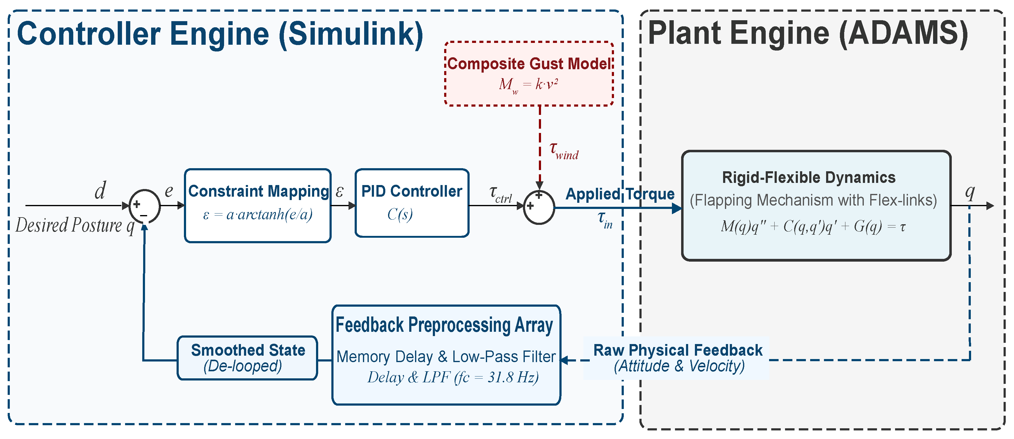
Simulink performs measurement, control calculation, and feedback processing, while ADAMS provides the flexible multibody plant, as shown in Figure 6. This division follows the controller–plant framework commonly used in multibody co-simulation [19,20].

In Figure 6, the target attitudes are compared with ADAMS feedback to generate joint errors. These errors enter error_warped fcn, where the diffeomorphic mapping is executed before four independent PID-type controllers compute the controller-command torques.

The controller-command torques are combined with environmental disturbance torques before entering ADAMS and are applied to the active joints through SFORCE elements. State variables are exported to scopes and the Workspace for analysis.

2.4.2. Distributed Weighted Injection of Complex Wind Loads and Feedback Noise-Suppression Mechanism

Steady wind, pulse gusts, and random noise are superimposed and converted into an equivalent aerodynamic dynamic-pressure signal proportional to the square of wind speed. Instead of applying a single concentrated torque, the signal is distributed across the active joints through decreasing weighting coefficients to reflect different moment arms under lateral wind excitation.

The communication step is 0.001 s. Each state-output channel uses a Memory delay and a first-order low-pass filter with a 31.83 Hz cutoff to break algebraic loops and attenuate flexible-body feedback noise. The interface variables, numerical settings, ADAMS 2024 runtime, and actuator-saturation logic are summarized in

Table 6. Key ADAMS–Simulink interface variables used in the rerun co-simulation.

Category	Variable or Channel	Direction	Unit/Rate
Torque input	CTRL_T2–CTRL_T5	Simulink to ADAMS SFORCE	N·mm, 1 kHz
Joint-angle feedback	VAR_Q2–VAR_Q5	ADAMS to Simulink	deg, 1 kHz
Wind disturbance	${\tau }_{w,i}$	Simulink disturbance model to torque summation	N·mm, 1 kHz
Torque logs	${\tau }_{unsat}$,${\tau }_{sat}$, saturation flags	Simulink logging	N·mm, 1 kHz
Plant torque	JOINT_i.TZ or SFORCE_i.TZ	ADAMS result database to post-processing	N·mm
Flexible response	PART_3_flex modal	Optional ADAMS result export	mm

,

Table 7. Co-simulation numerical settings and model-implementation characteristics.

Item	Setting
Plant model	Bird_5Link; PART_3_flex
Unit system	MMKS: mm, kg, N, s, deg
Flexible-body modes	1108 nodes; 24 modes; retained elastic modes 7–24
Passive joint	JOINT_1 with FRICTION_1; preload torque 150 N·mm
Active torque interface	CTRL_T2–CTRL_T5 driving ADAMS SFORCE elements
Communication step	$T_s=0.001$ s; nominal data-exchange rate 1 kHz
Feedback conditioning	Memory block plus $G_f\left(s\right)=1/(0.005s+1)$ low-pass filter
Mechanical hard stop	No explicit hard-stop element in the exported ADAMS text model
Actuator saturation	Simulink-side saturation before ADAMS input; nominal bound $\pm 45$ N·mm

and

Table 8. Actuator saturation and anti-windup implementation.

Controller/Interface	Torque Bound	Location
PID	$\pm 45$ N·mm per active joint	Before CTRL_T2–CTRL_T5
SMC	$\pm 45$ N·mm per active joint	Before ADAMS input
Proposed	$\pm 45$ N·mm per active joint	After mapped-error controller and before ADAMS input
ADAMS SFORCE interface	No independent actuator limit	ADAMS plant side

.

3. Results

The proposed controller is evaluated under increasingly demanding ADAMS–Simulink scenarios. Conventional PID is used as the basic linear reference, and sliding mode control (SMC) is added as a robust nonlinear baseline because it is widely used under uncertainties and disturbances but may introduce switching chattering [27].

3.1. Trajectory Tracking and Suppression of the Flexible Whip-like Effect Under Ideal Wind-Free Conditions

The first experiment removes external wind to isolate rigid–flexible coupling. The active joints track the nominal step targets of ${40}^{\circ }$, $-{20}^{\circ }$, ${15}^{\circ }$, and $0^{\circ }$ for joints 2–5.

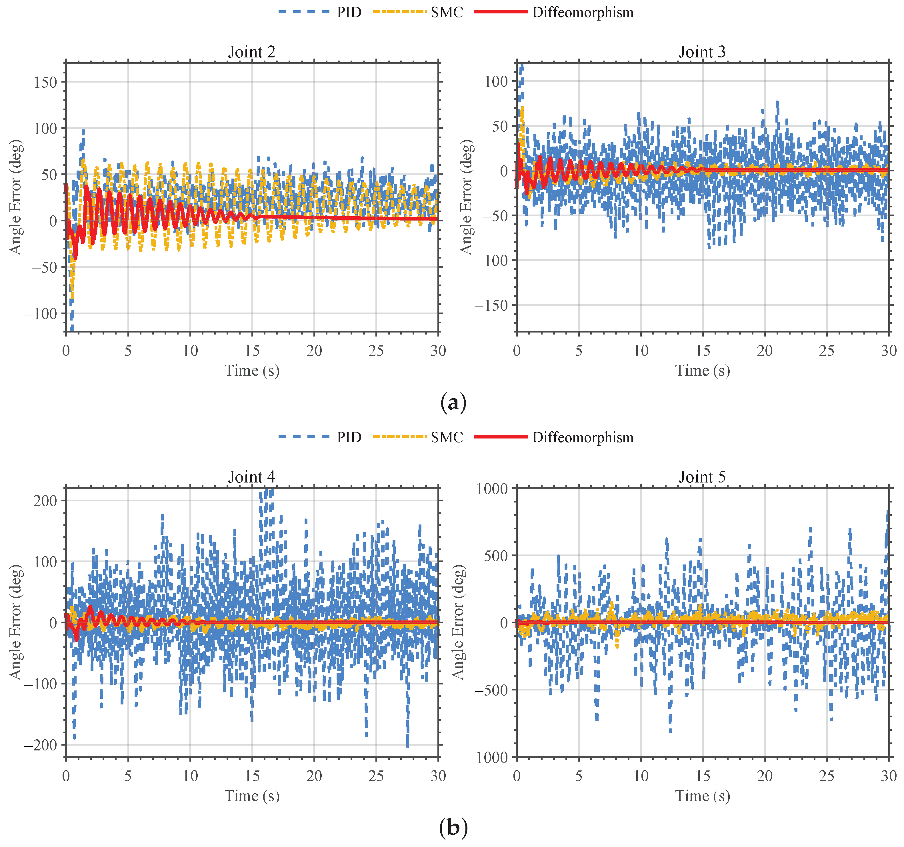
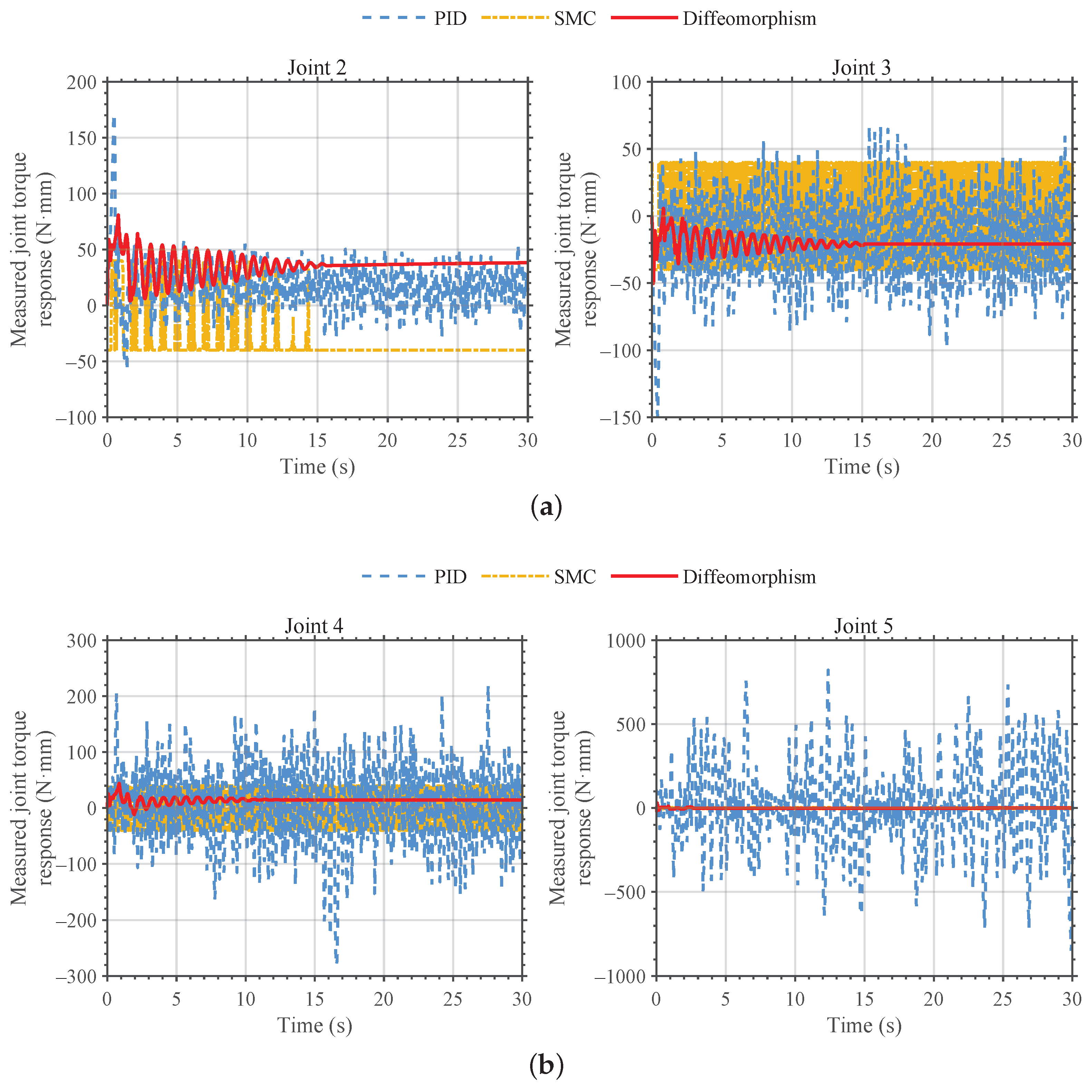
Under wind-free conditions, PID still produces large joint-error oscillations, especially at distal joints 4 and 5 (Figure 7). The measured torque responses also fluctuate strongly (Figure 8), indicating that rigid-body PID feedback amplifies flexible link vibration instead of separating it from macroscopic tracking error [28].

SMC reduces the error amplitude relative to PID, consistent with its robustness to matched disturbances [27]. However, residual oscillations and switching-related torque variations remain (Figure 7 and Figure 8), so the measured vibration-related response is not fully attenuated.

The proposed controller reduces error oscillations and avoids the high-frequency torque bursts of PID and the chattering of SMC. This supports the intended mechanism: smooth small-error regulation and stronger nonlinear correction near the prescribed boundary [12,13]. The performance metrics are summarized in

Table 9. Performance metrics comparison of the three control strategies under wind-free conditions.

Performance Metric	Conventional PID	SMC	Proposed Diffeomorphism
Settling time $t_s$/s	Not converged	Not converged	28.31
Maximum attitude deviation error/°	848.06	187.23	41.00
RMSE/°	137.70	27.62	7.25
Recovery time $t_r$/s	Not recovered	Not recovered	27.54
Peak measured joint torque response/N·mm	848.06	40.00	80.78
Constraint violation	Yes	Yes	No
Measured-channel spectral peak/dB	42.22	19.63	10.90

; torque-related metrics denote ADAMS-side measured joint torque responses rather than saturated Simulink command torques.

The wind-free results support three observations:

1.

PID and SMC do not converge, whereas the proposed controller achieves the lowest RMSE ($7.{25}^{\circ }$), lowest maximum deviation ($41.{00}^{\circ }$), and convergence within about 30 s.

2.

PID reaches a peak measured joint torque response of 848.06 N·mm. SMC lowers the torque response but still violates the boundary. The proposed controller keeps the response at 80.78 N·mm with smoother dynamics.

3.

The measured-channel spectral peak decreases from 42.22 dB under PID to 19.63 dB under SMC and 10.90 dB under the proposed controller.

Thus, even without wind loading, flexible link feedback can destabilize boundary-blind controllers. The proposed controller provides a better balance among convergence, measured torque-response smoothness, and boundary protection.

3.2. Physical Boundary Protection and Transient Recovery Under Transient Pulse Compound Crosswind Disturbance

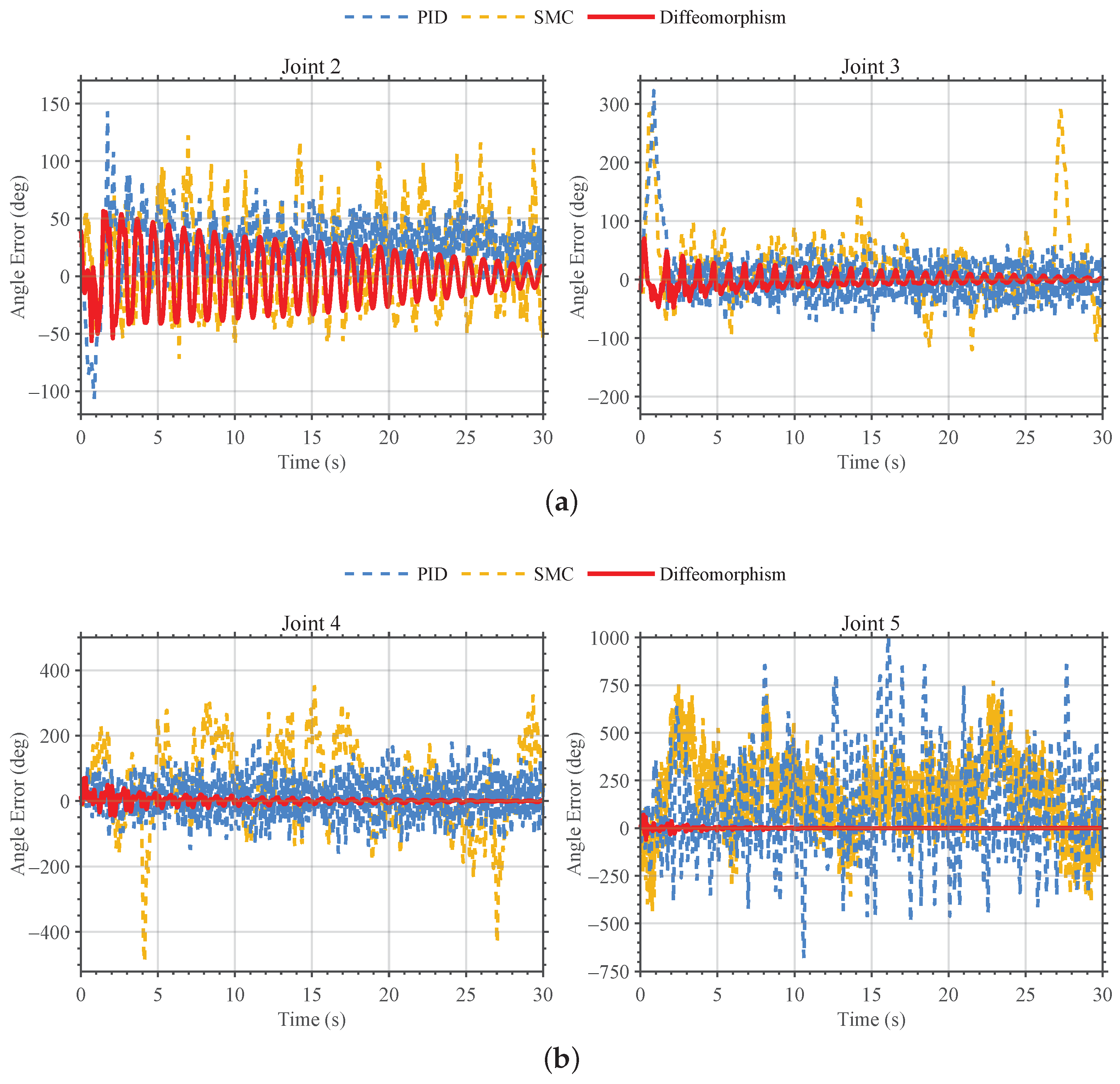
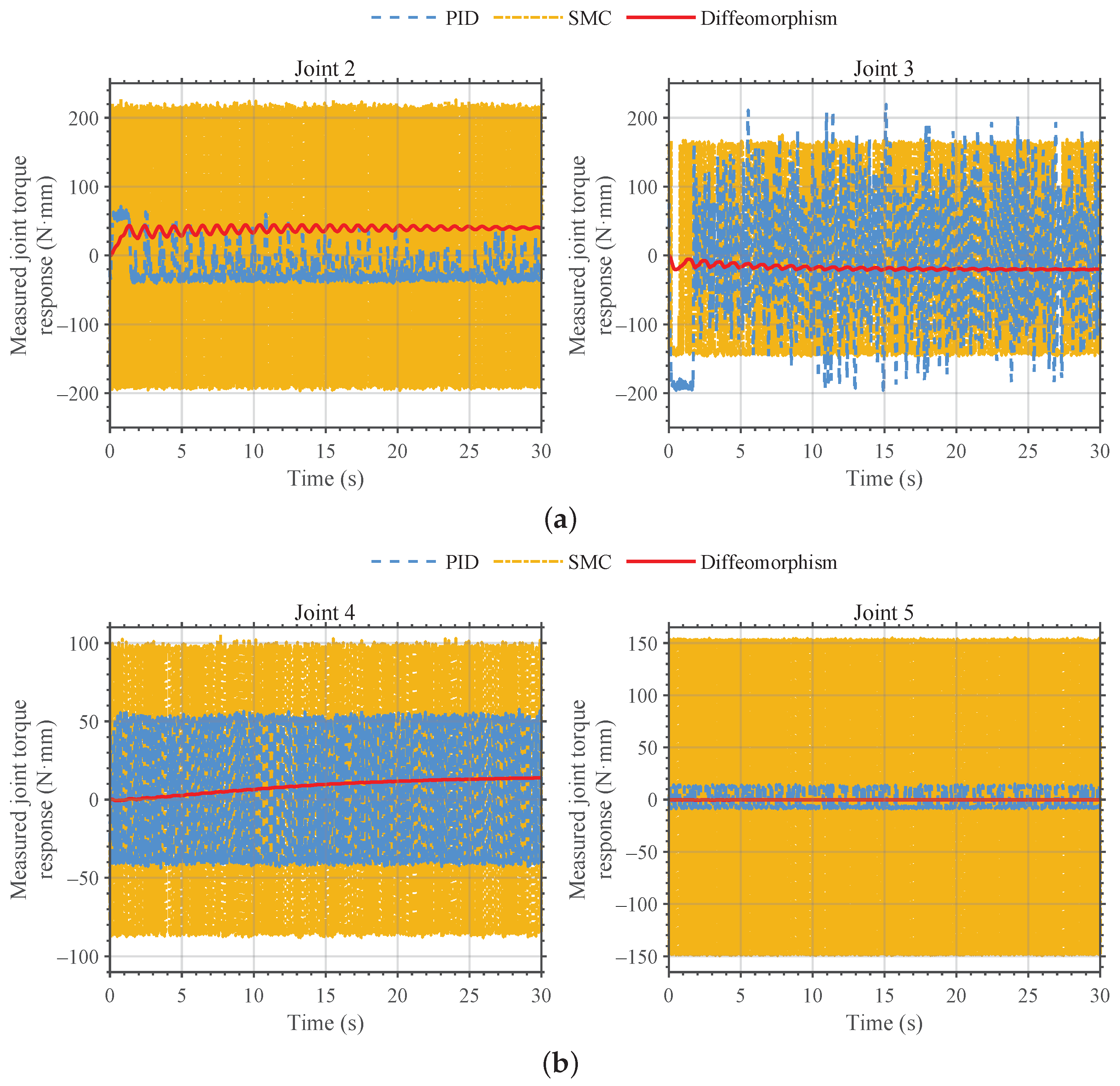
The pulse wind experiment uses a 2 m/s steady wind with white noise and a 1 m/s pulse during 50–52 s. The equivalent disturbance torque increases from approximately 12.37 to 27.35 N·mm. Figure 9 and Figure 10 compare attitude error and measured-torque responses under PID, SMC, and the proposed controller.

PID shows large post-pulse oscillations and does not recover after the disturbance ends. SMC reduces the error relative to PID but still exhibits strong fluctuations and limited recovery. The proposed controller keeps all four joint errors in a small range and avoids excessive measured-torque bursts, showing stronger transient recovery and boundary protection. Quantitative metrics are summarized in

Table 10. Performance metrics comparison of the three control strategies under a 2 m/s steady wind with a 1 m/s pulse disturbance.

Performance Metric	Conventional PID	SMC	Proposed Diffeomorphism
Settling time $t_s$/s	Not converged	Not converged	6.15
Maximum angular excursion/°	1602.56	381,330.03	23.58
RMSE/°	491.7	224,400	2.943
Recovery time $t_r$/s	Not recovered	Not recovered	0
Peak measured joint torque response/N·mm	46.42	34.73	136.3
Constraint violation	Yes	Yes	No
Frequency-domain evidence	See Table 12	See Table 12	See Table 12

.

The pulse wind results support three observations:

1.

Boundary protection. PID and SMC reach runaway unwrapped angular excursions of $1602.{56}^{\circ }$ and $381330.{03}^{\circ }$, respectively. The proposed controller remains at $23.{58}^{\circ }$ with an RMSE of $2.{943}^{\circ }$ and no boundary violation.

2.

Measured torque response. PID and SMC have lower peak measured torque responses, 46.42 and 34.73 N·mm, but these do not produce recovery. The proposed controller uses a bounded stabilizing response of 136.3 N·mm while maintaining safety.

3.

Frequency-domain evidence. The frequency interpretation is restricted to exported feedback and torque-response channels. The supplemental spectra show lower measured-channel excitation for the proposed method without the runaway response seen in PID and SMC.

Under the 2 m/s steady wind with a 1 m/s pulse, PID fails and SMC remains insufficient, while the proposed controller preserves the safety boundary and achieves bounded recovery under the same torque-limited conditions.

3.3. Statistical Robustness Analysis Based on Two-Dimensional Parameter Scanning

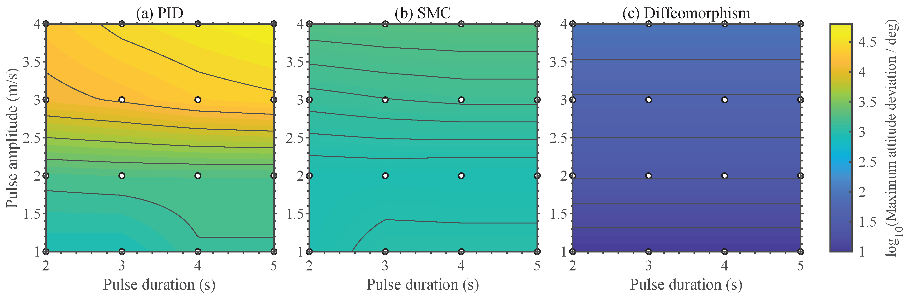
To test robustness beyond one operating point, pulse wind amplitude was varied from 1 to 4 m/s and pulse duration from 2 to 5 s at a fixed 2 m/s steady wind, giving 16 disturbance combinations. Figure 11 maps ${\log }_{10}\left(\mathrm{Max}\mathrm{Error}\right)$, where yellow indicates higher error and blue indicates lower error.

PID is highly sensitive to both pulse amplitude and duration, with errors reaching the order of ${10}^4$ under 3–4 m/s pulse disturbances. SMC gives a smoother surface but remains mainly at the order of ${10}^3$. The proposed controller keeps the maximum deviation mainly within ${10}^1$–${10}^2$ and varies more smoothly as disturbance severity increases. Thus, the method does not rely on a single tuned condition and maintains constrained stability over the scanned disturbance range [26].

3.4. Sensitivity and Design Trade-Off Analysis of the Mapping Parameter a

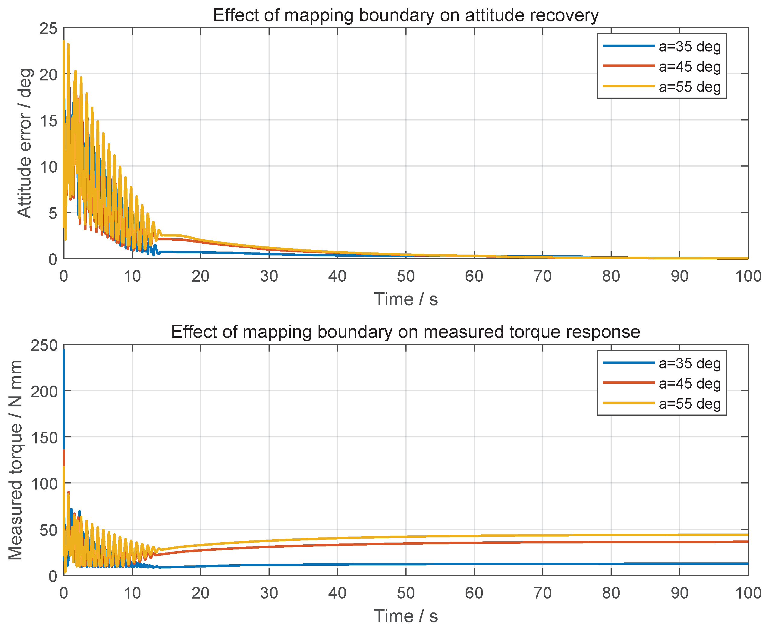
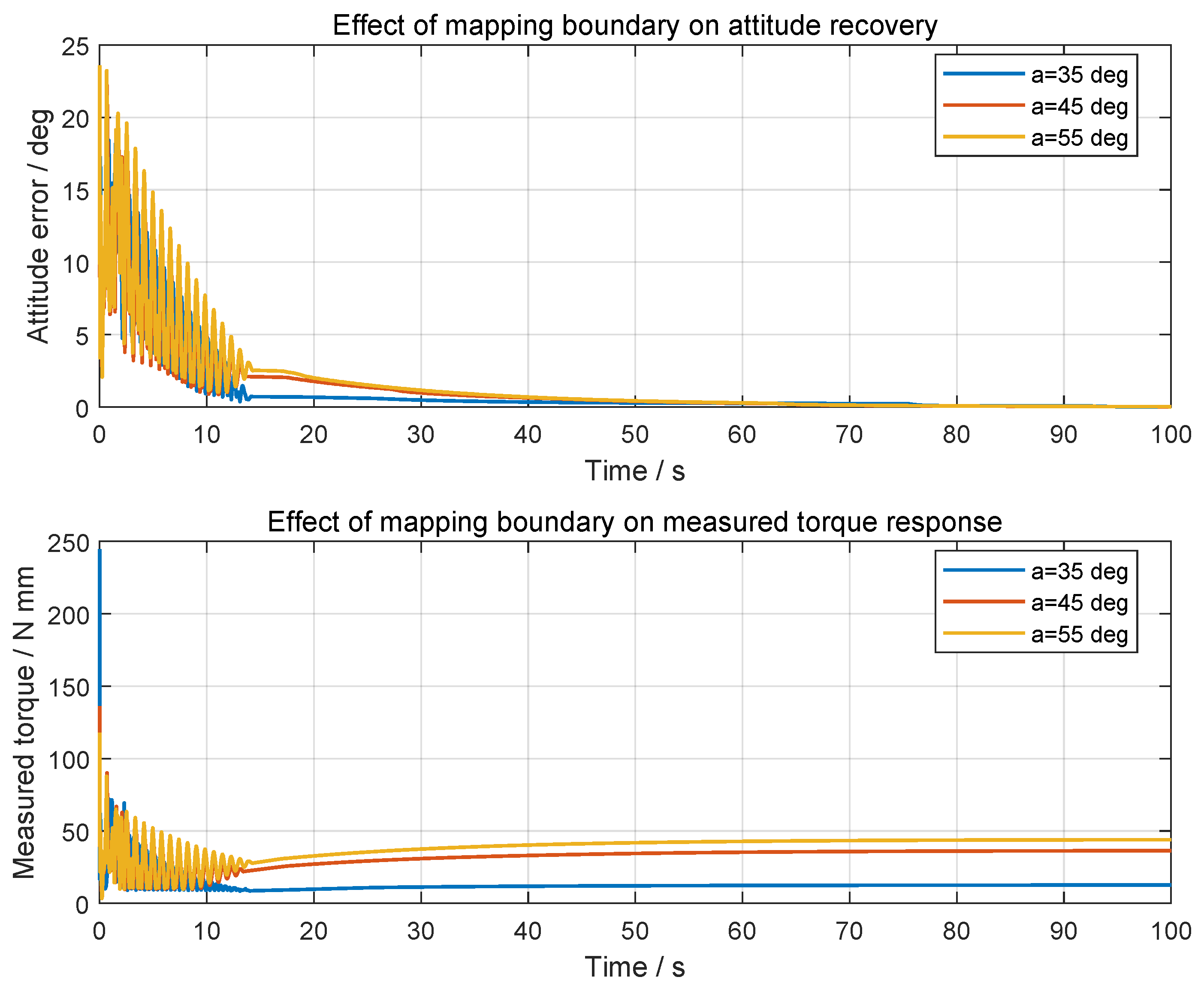
The sensitivity analysis varies only the mapping boundary parameter, $a={35}^{\circ }$, ${45}^{\circ }$, and ${55}^{\circ }$, under the same 1 m/s pulse wind condition. Figure 12 and

Table 11. Comparison of rerun system performance metrics under different mapping parameters a.

Performance Metric	$\mathit{a}={35}^{\circ }$	$\mathit{a}={45}^{\circ }$	$\mathit{a}={55}^{\circ }$
Maximum angular excursion/°	23.58	23.58	23.58
RMSE/°	2.829	2.943	3.251
Recovery time $t_r$/s	0	0	0
Peak measured joint torque response/N·mm	244.5	136.3	117.9
Torque RMS/N·mm	14.32	33.02	39.74
Saturation duration/s	0.994	1.098	1.683
Constraint violation	No	No	No
High-frequency torque PSD integral	482.2	106.5	66.19

compare angular response, measured torque response, and measured-channel spectral characteristics over the full pulse-and-recovery interval.

All three values keep the maximum angular excursion at $23.{58}^{\circ }$ with no boundary violation. The RMSE values are $2.{829}^{\circ }$, $2.{943}^{\circ }$, and $3.{251}^{\circ }$, and the recovery time is 0 s under the adopted criterion. The measured torque response is more sensitive to a: the peak measured torque decreases from 244.5 to 136.3 and 117.9 N·mm as a increases, while torque RMS increases from 14.32 to 39.74 N·mm. The high-frequency torque PSD integral also decreases from 482.2 to 106.5 and 66.19. These exported-channel metrics indicate that $a={45}^{\circ }$ provides a practical balance among error accuracy, peak torque response, torque RMS, high-frequency content, and boundary safety.

3.5. Frequency-Domain, Sensitivity, and Baseline Analyses

3.5.1. Measured-Channel Frequency-Domain Evidence

The ADAMS–Simulink interface exports joint-response and torque-response channels, but not all modal coordinates or flexible-tip displacement channels. The frequency-domain results are therefore measured-channel evidence rather than direct proof of suppression of every higher-order elastic mode. With $T_s=0.001$ s, the nominal Nyquist frequency is 500 Hz, whereas the lowest parsed elastic modal frequency is 5865.665 Hz.

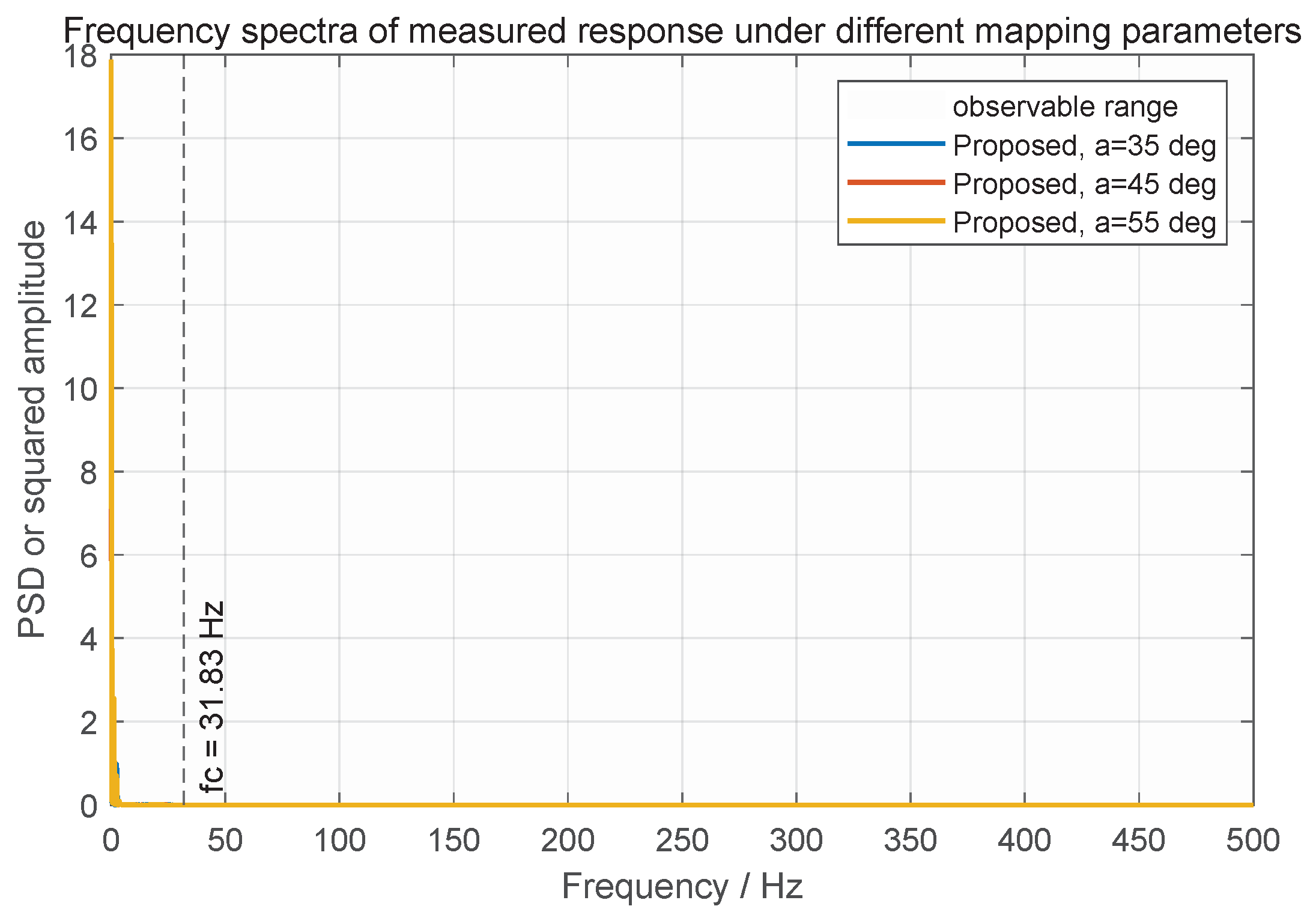
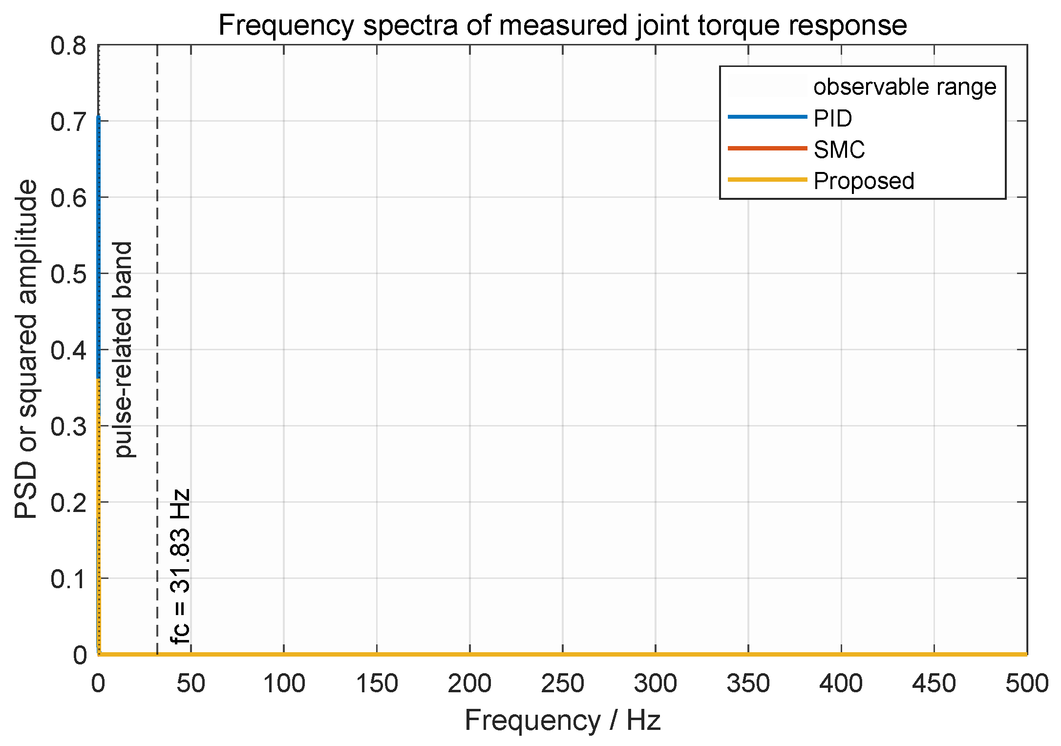
Figure 13 and Figure 14 compare the measured-response and measured joint-torque spectra, respectively. The gray region denotes the nominal observable frequency range up to 500 Hz, the dashed vertical line marks the 31.83 Hz feedback-filter cutoff, and the dotted line in Figure 14 identifies the pulse-related frequency band.

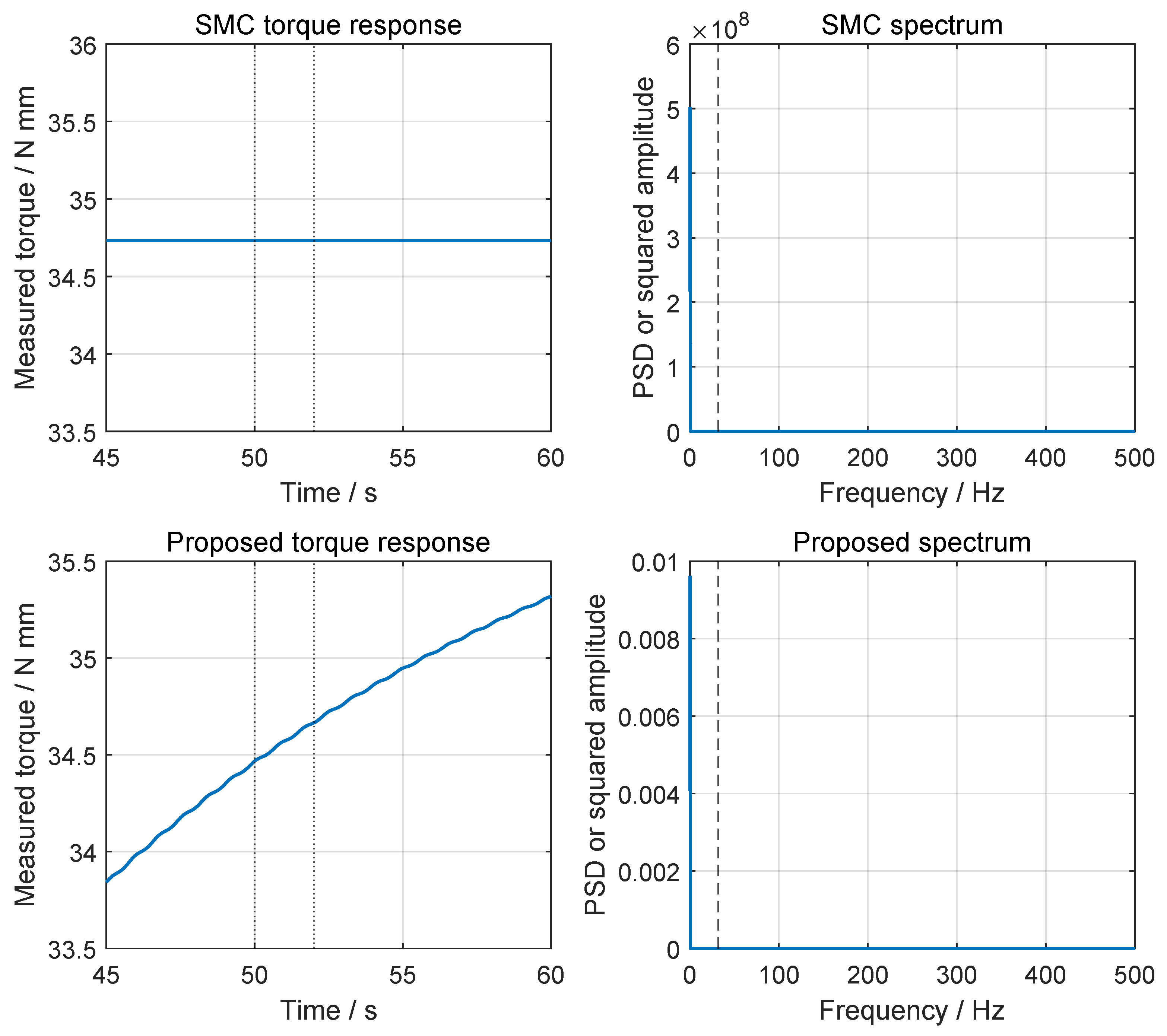
With the current Simulink communication step of 0.001 s, the nominal sampling frequency is 1000 Hz and the Nyquist frequency is 500 Hz. The lowest parsed elastic modal frequency is 5865.665 Hz, which is above the 500 Hz Nyquist frequency. Therefore, claims about high-order modal resonance must be limited to the measured feedback band unless higher-rate modal coordinate logs are exported. Figure 15 shows the local time–frequency response; dotted vertical lines in the left panels mark the 50–52 s pulse interval, and dashed lines in the right panels mark the 31.83 Hz filter cutoff.

Table 12. Dominant spectral components of measured response and joint-torque signals.

Case	Interval	Frequency/Hz	Peak Amplitude
Proposed, $a={35}^{\circ }$	0–100 s	1.221; 2.441; 3.662	0.1302; 0.9692; 0.02492
Proposed, $a={45}^{\circ }$	0–100 s	1.221; 2.441; 3.662	1.675; 0.5395; 0.05749
Proposed, $a={55}^{\circ }$	0–100 s	1.221; 2.441; 3.662	2.553; 0.6949; 0.0854
PID	45–60 s	0.488; 0.684; 0.879	0.004879; 0.002807; 0.001397
SMC	45–60 s	0.244; 0.488; 0.732	near noise floor
Proposed, nominal	45–60 s	1.221	$5.141\times {10}^{-5}$

summarizes the dominant components in the measured-response and measured joint-torque spectra.

3.5.2. Parameter Selection and Gain Sensitivity

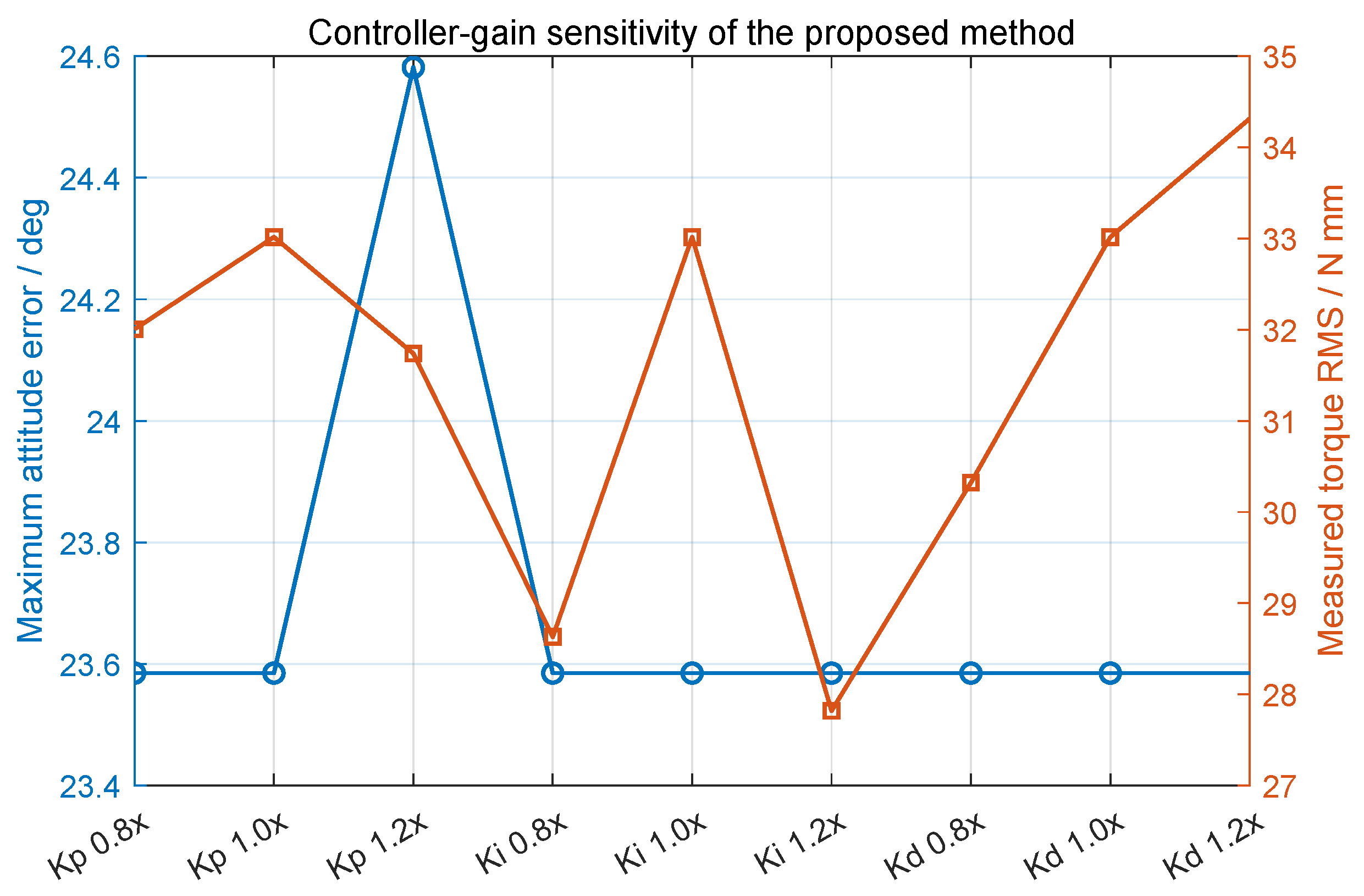
All mapping-boundary reruns remain inside the prescribed boundary. For $a={35}^{\circ }$, ${45}^{\circ }$, and ${55}^{\circ }$, the maximum angular excursion is 23.58°, and the RMSE values are 2.829°, 2.943°, and 3.251°. As a increases, the high-frequency torque PSD integral decreases but torque RMS increases; $a={45}^{\circ }$ is retained as the nominal compromise.

Table 13. Parameter-selection and sensitivity results from synchronized reruns.

Case	Varied	Max./deg	RMSE/deg	Peak Torque	RMS	Sat./s	Violation	PSD
$a={35}^{\circ }$	a	23.58	2.829	244.5	14.32	0.994	No	482.2
$a={45}^{\circ }$	a	23.58	2.943	136.3	33.02	1.098	No	106.5
$a={55}^{\circ }$	a	23.58	3.251	117.9	39.74	1.683	No	66.19
$K_p$ 0.8×	$K_p$	23.58	3.314	118.5	32.00	0.961	No	75.72
$K_p$ 1.0×	$K_p$	23.58	2.943	136.3	33.02	1.098	No	106.5
$K_p$ 1.2×	$K_p$	24.58	2.922	154.8	31.74	1.241	No	150.5
$K_i$ 0.8×	$K_i$	23.58	2.866	136.3	28.63	0.887	No	113.8
$K_i$ 1.0×	$K_i$	23.58	2.943	136.3	33.02	1.098	No	106.5
$K_i$ 1.2×	$K_i$	23.58	2.753	136.3	27.82	0.882	No	115.6
$K_d$ 0.8×	$K_d$	23.58	2.893	127.6	30.32	0.900	No	100.8
$K_d$ 1.0×	$K_d$	23.58	2.943	136.3	33.02	1.098	No	106.5
$K_d$ 1.2×	$K_d$	23.58	2.933	145.7	34.32	1.181	No	117.2

summarizes the synchronized reruns, while Figure 16 and Figure 17 show the boundary-parameter and controller-gain sensitivity results, respectively.

The one-factor gain sweep uses 0.8, 1.0, and 1.2 times the nominal $K_p$, $K_i$, and $K_d$ values. All cases remain inside the 45° boundary; only $K_p=1.2$ increases the maximum response to 24.58°. The measured torque RMS is 27.82–34.32 N·mm.

3.5.3. Runaway Excursion and CBF-QP Baseline

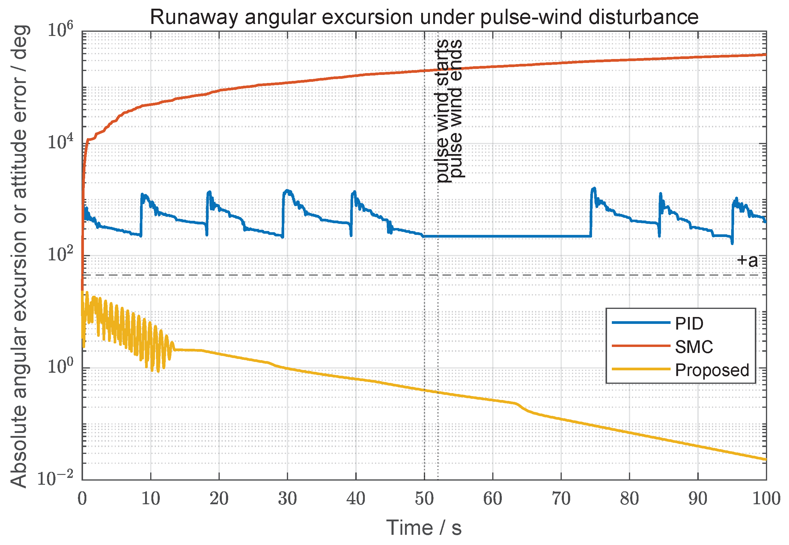
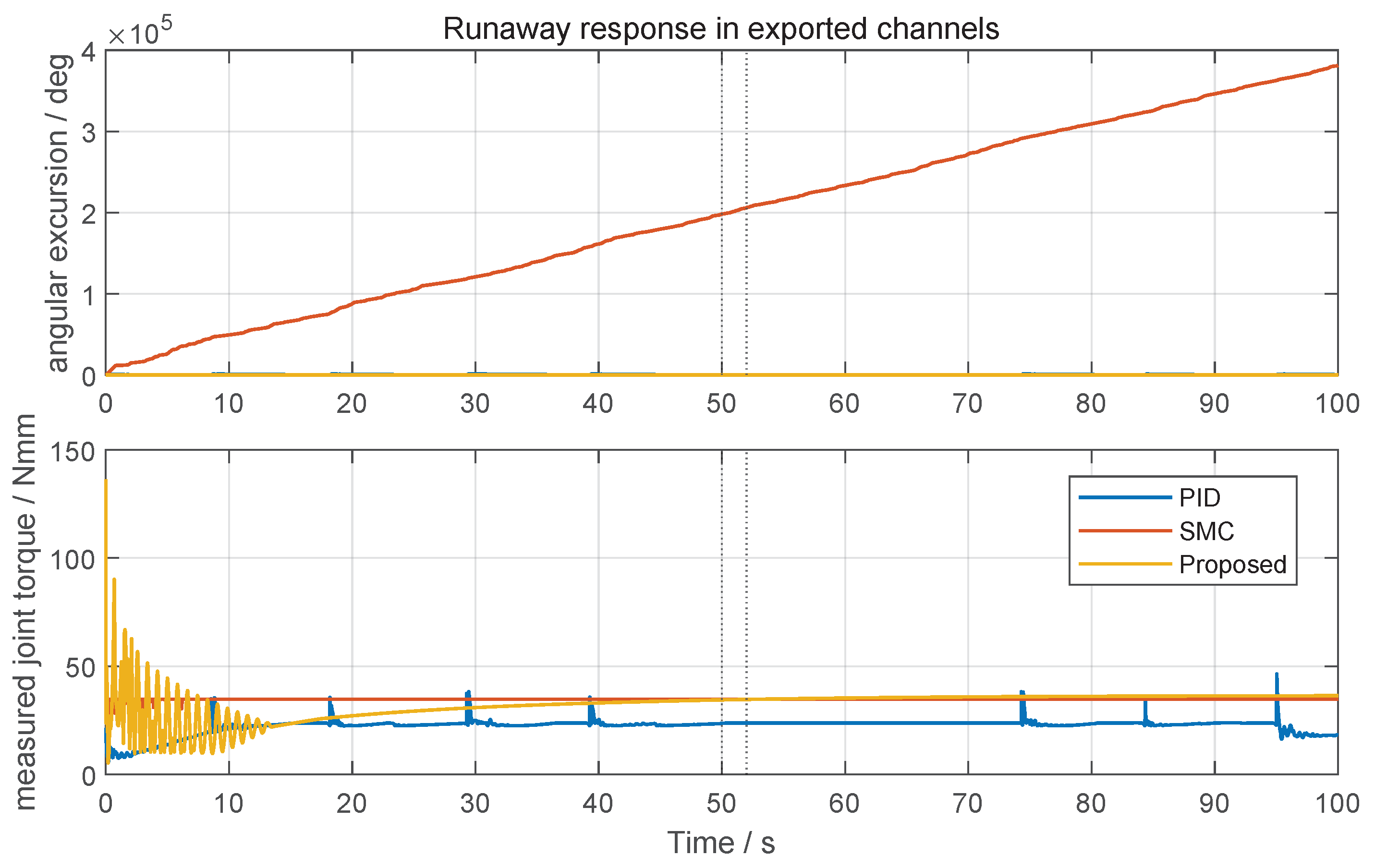
The PID and SMC reruns show runaway unwrapped angular excursions of 1602.56° and 381,330.03°, respectively. These values indicate instability rather than ordinary bounded attitude errors. The proposed nominal case remains bounded at 23.58°. Figure 18 compares the unwrapped excursions, and Figure 19 shows the corresponding response-level behavior.

Table 14. Physical interpretation of large angular deviations.

Controller	Maximum Unwrapped Angular Excursion	Boundary Violation	Physical Meaning
PID	1602.56°	Yes	Runaway angular excursion after loss of stability; no mechanical hard stop is defined in the exported plant.
SMC	381,330.03°	Yes	Runaway angular excursion after loss of stability; the value is not a normal bounded attitude error.
Proposed	23.58°	No	Bounded response inside the prescribed safety boundary in the exported log.

summarizes their physical interpretation.

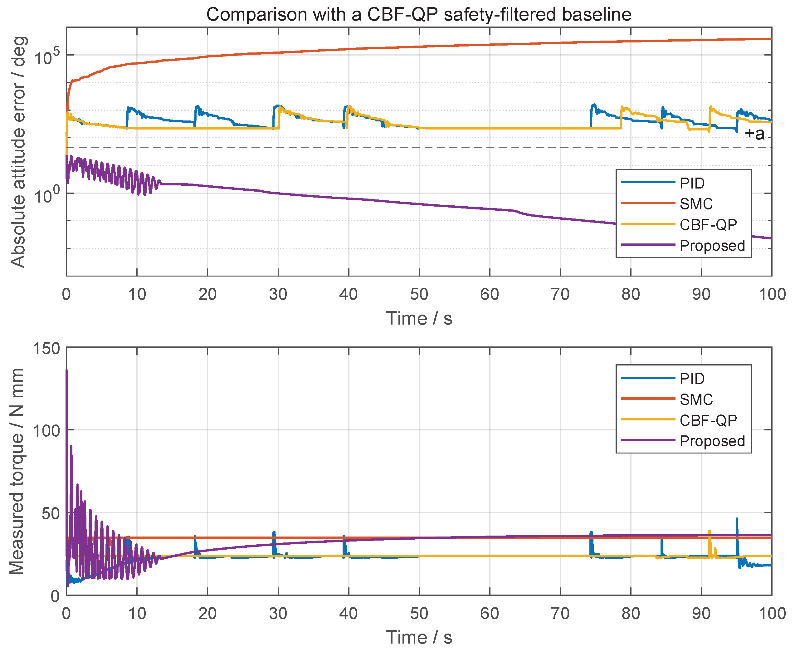
A CBF-QP safety-filtered PID baseline was rerun using the same $\pm 45\mathrm{N}\mathrm{mm}$ torque bound. It still violates the boundary, with an RMSE of 577° and a maximum angular excursion of 1394°, whereas the proposed controller remains inside the prescribed boundary. Figure 20 compares the controller responses, and

Table 15. Comparison with baseline constrained-control methods.

Controller	Violation	RMSE	Max. Excursion/Peak Torque	Interpretation
PID	Yes	491.7	1603°/46.42 N·mm	Unconstrained baseline; boundary is lost after disturbance.
SMC	Yes	$2.244\times {10}^5$	$3.813\times {10}^5$ deg/34.73 N·mm	Switching baseline; command bound alone does not prevent runaway rotation.
Safety-filtered PID	Yes	577	1394°/38.99 N·mm	Constraint-aware filter is insufficient under the torque-limited rerun condition.
Proposed	No	2.943	23.58°/136.3 N·mm	Boundary-aware error reshaping keeps the response inside the prescribed limit.

summarizes the constrained-control baselines.

4. Discussion

The simulations show that instability arises from the interaction among structural flexibility, passive-joint friction constraints, wind disturbances, and closed-loop control inputs. Even without wind, the flexible leg link can excite high-frequency responses during step tracking, which conventional PID feedback further amplifies. Thus, rigid-body assumptions are insufficient for lightweight perching systems with slender load-bearing links.

Compared with PID and SMC, the proposed controller better balances tracking accuracy, measured torque-response smoothness, measured-channel flexible-excitation attenuation, and boundary protection. Its inverse hyperbolic tangent mapping is smooth for small errors and strongly amplifies errors near the boundary. This explains the attenuation of measured feedback/torque-channel oscillations and the absence of boundary violation under wind-free and pulse wind conditions.

The two-dimensional scan shows that the method is not limited to one tuned disturbance case. The sensitivity analysis further indicates that a weakly affects error response and recovery within 35–${55}^{\circ }$, but strongly affects measured torque response. Thus, a is a practical design parameter for balancing boundary strength, torque variation, and measured-channel high-frequency attenuation.

The following discussion clarifies implementation cost, modeling scope, and future hardware-validation needs.

4.1. Computational Feasibility of the Diffeomorphic Mapping

The controller evaluates

$${ϵ}_i=a\mathrm{arctanh}\left({\displaystyle \frac{e_i}{a}}\right)$$

(29)

for four active joints at the 1 kHz co-simulation update rate. This requires only four inverse-hyperbolic evaluations per step. For practical implementation, the normalized input should be clipped before evaluating the mapping:

$${\xi }_i=\mathrm{clip}\left({\displaystyle \frac{e_i}{a}},-1+\delta ,1-\delta \right),{ϵ}_i=a\mathrm{arctanh}\left({\xi }_i\right).$$

(30)

This clipping avoids numerical singularities and can be logged as a boundary-proximity indicator. Floating-point implementation is feasible in principle for modern embedded processors, while lookup-table or polynomial approximations can support lower-cost controllers. Verified onboard timing and hardware-in-the-loop validation remain future work.

4.2. Model Assumptions, Limitations, and Future Work

The conclusions are based on ADAMS–Simulink co-simulation, not prototype experiments. The wind field is represented by equivalent disturbance torques rather than high-fidelity unsteady CFD. The flexible link is an MNF-based reduced flexible body, and the default interface does not export all flexible tip or modal coordinate channels.

ADAMS SFORCE elements are torque–input interfaces, not complete motor drive models. Motor current dynamics, voltage limits, thermal effects, backlash, current-loop delay, sensor quantization, and hardware communication delays are not fully represented. Actuator amplitude constraints and anti-windup logic are therefore implemented in Simulink before the torque command enters ADAMS.

Large PID and SMC joint-angle values are runaway unwrapped angular excursions after loss of stability because the exported plant has no explicit mechanical hard stops. The proposed controller also does not directly measure or actuate flexible modal coordinates, so the flexible-response claim is limited to measured feedback and torque channels. Future work will add hardware-in-the-loop experiments, motor drive modeling, mechanical hard stops, direct flexible-response sensing where feasible, and prototype validation under controlled wind disturbances.

5. Conclusions

A diffeomorphism-based attitude-constrained controller was developed for a rigid–flexible coupled flapping-wing robot and evaluated in ADAMS–Simulink co-simulation [12,13,19,20]. By mapping constrained physical attitude errors into an unconstrained virtual space, the method improves nonlinear regulation near the safety boundary. The main conclusions are:

1.

The diffeomorphism-based controller improves wind-free trajectory tracking. PID amplifies high-frequency measured-channel components from the flexible link, and SMC leaves residual oscillation and boundary violation. The proposed controller gives better convergence and smoother measured torque response.

2.

The proposed method improves pulse wind disturbance rejection. Under a 2 m/s steady wind with a 1 m/s pulse, PID and SMC show runaway angular excursion and boundary violation. The CBF-QP safety-filtered PID baseline also violates the boundary, whereas the proposed controller remains bounded.

3.

The parameter scan verifies robustness across disturbance combinations. Across 16 pulse-amplitude and duration cases, PID degrades rapidly and SMC remains at high-error levels, while the proposed controller maintains lower error levels.

4.

The mapping parameter a mainly tunes measured torque response. For $a={35}^{\circ }$, ${45}^{\circ }$, and ${55}^{\circ }$, the boundary-protection conclusion is unchanged, but peak measured torque and torque RMS vary noticeably. Thus, a tunes the trade-off between boundary intensity and response-level torque variation.

5.

The proposed controller gives the best overall simulation performance. Compared with PID, SMC, and CBF-QP safety-filtered PID baselines, it reduces attitude deviation, avoids boundary violation, and weakens high-frequency measured-channel influence under rigid–flexible coupling and wind disturbance.

References

1. Zufferey, R.; Tormo-Barbero, J.; Feliu-Talegn, D.; Rafee Nekoo, S.; Acosta, J.; Ollero, A. How ornithopters can perch autonomously on a branch. Nat. Commun. 2022, 13, 7713. [Google Scholar] [CrossRef] [PubMed]
2. Wu, X.; Sun, W.; Sun, W.; Zhu, C.; Zhang, X. Research progress on autonomous landing methods for micro non-fixed-wing UAVs. Tech. Autom. Appl. 2024, 43, 1–6+23. [Google Scholar] [CrossRef]
3. Zhang, C. Design and Dynamic Simulation of a Bionic Bird Autonomous Jumping Mechanism. Master Thesis, Shenyang Ligong University, Shenyang, China, 2024. [Google Scholar]
4. Zufferey, R.; Tormo-Barbero, J.; Guzmn, M.M.; Maldonado, F.J.; Sanchez-Laulhe, E.; Grau, P.; Perez, M.; Acosta, J.; Ollero, A. Design of the high-payload flapping wing robot E-Flap. IEEE Robot. Autom. Lett. 2021, 6, 3097–3104. [Google Scholar] [CrossRef]
5. Gomez-Tamm, A.E.; Perez-Sanchez, V.; Arrue, B.C.; Ollero, A. SMA actuated low-weight bio-inspired claws for grasping and perching using flapping wing aerial systems. In Proceedings of the IEEE/RSJ International Conference on Intelligent Robots and Systems (IROS), Las Vegas, NV, USA, 24 October–24 January 2021; pp. 1–6. [Google Scholar] [CrossRef]
6. Zhang, C.; Shao, W.; Hao, Y. A bionic bird jumping grasping structure design based on stm32 development board control. Sci. Rep. 2024, 14, 10435. [Google Scholar] [CrossRef] [PubMed]
7. Wang, B.; Yin, H.; Zi, P.; Xu, K.; Tian, Y.; Lyu, S.; Ding, X. Bionic bird claw design for grabbing and perching inspired by tendon-locking mechanism. IEEE Robot. Autom. Lett. 2024, 9, 8090–8097. [Google Scholar] [CrossRef]
8. Broers, K.C.V.; Armanini, S.F. Design and testing of a bioinspired lightweight perching mechanism for flapping-wing MAVs using soft grippers. IEEE Robot. Autom. Lett. 2022, 7, 7526–7533. [Google Scholar] [CrossRef]
9. Zhu, Y.; He, X.; Zhang, P.; Guo, G.; Zhang, X. Perching and grasping mechanism inspired by a bird claw. Machines 2022, 10, 656. [Google Scholar] [CrossRef]
10. Nabi, F.G.; Sundaraj, K.; Vijean, V.; Shafiq, M.; Palaniappan, R.; Talib, I.; Rehman, H.U. A novel design of robotic hand based on bird claw model. J. Phys. Conf. Ser. 2021, 1997, 012034. [Google Scholar] [CrossRef]
11. Guo, S.; Xu, Y.; Sun, W.; Liu, L. Under-Actuated Grasping Mechanical Arm Mechanism of Bird-like Arm Claw. Chinese Patent CN118024221A, 14 May 2024. [Google Scholar]
12. Acosta, J.; Dria-Cerezo, A.; Fossas, E. Stabilisation of state-and-input constrained nonlinear systems via diffeomorphisms. Int. J. Robust Nonlinear Control 2018, 28, 4032–4044. [Google Scholar] [CrossRef]
13. Acosta, J.; Dria-Cerezo, A.; Fossas, E. Diffeomorphism-based control of nonlinear systems subject to state constraints with actual applications. In Proceedings of the 2014 IEEE Conference on Control Applications (CCA), Juan Les Antibes, France, 8–10 October 2014; pp. 923–928. [Google Scholar] [CrossRef]
14. Meng, Q.; Lai, X.; Yan, Z.; Wu, M. Tip position control and vibration suppression of a planar two-link rigid-flexible underactuated manipulator. IEEE Trans. Cybern. 2022, 52, 6771–6783. [Google Scholar] [CrossRef] [PubMed]
15. Kim, D.W.; Kwak, M.K.; Kim, S.-M.; Feeny, B.F. Slewing and active vibration control of a flexible single-link manipulator. Actuators 2025, 14, 43. [Google Scholar] [CrossRef]
16. Zhang, Q.; Zhao, X.; Liu, L.; Dai, T. Adaptive sliding mode neural network control and flexible vibration suppression of a flexible spatial parallel robot. Electronics 2021, 10, 212. [Google Scholar] [CrossRef]
17. Feliu-Talegon, D.; Acosta, J.; Ollero, A. Control aware of limitations of manipulators with claw for aerial robots imitating bird’s skeleton. IEEE Robot. Autom. Lett. 2021, 6, 6426–6433. [Google Scholar] [CrossRef]
18. Feliu-Talegon, D.; Acosta, J.; Suarez, A.; Ollero, A. A bio-inspired manipulator with claw prototype for winged aerial robots: Benchmark for design and control. Appl. Sci. 2020, 10, 6516. [Google Scholar] [CrossRef]
19. Chattopadhyay, P.; Dikshit, H.; Majumder, A.; Ghoshal, S.; Maity, A. Dynamic analysis of a bio-inspired climbing robot using ADAMS-SIMULINK co-simulation. AIP Conf. Proc. 2018, 1952, 020015. [Google Scholar] [CrossRef]
20. Liu, T.; Zhang, Z.; Liu, Y.; Fan, X. Motion simulation of bionic hexapod robot based on ADAMS/MATLAB co-simulation. J. Phys. Conf. Ser. 2020, 1601, 062032. [Google Scholar] [CrossRef]
21. Shabana, A.A. Flexible multibody dynamics: Review of past and recent developments. Multibody Syst. Dyn. 1997, 1, 189–222. [Google Scholar] [CrossRef]
22. Abbood, I.S.; Odaa, S.A.; Hasan, K.F.; Jasim, M.A. Properties evaluation of fiber reinforced polymers and their constituent materials used in structures—A review. Mater. Today Proc. 2021, 43, 1003–1008. [Google Scholar] [CrossRef]
23. ACP Composites, Inc. Mechanical Properties of Carbon Fiber Composite Materials; Product Specification Reference Sheet; ACP Composites, Inc.: Livermore, CA, USA, 2012; Available online: https://acpcomposites.com/wp-content/uploads/2023/12/Mechanical-Properties-of-Carbon-Fiber-Composite-Materials.pdf (accessed on 8 July 2026).
24. Craig, R.R.; Bampton, M.C.C. Coupling of substructures for dynamic analyses. AIAA J. 1968, 6, 1313–1319. [Google Scholar] [CrossRef] [PubMed]
25. Langelaan, J.W.; Alley, N.; Neidhoefer, J. Wind field estimation for small unmanned aerial vehicles. In Proceedings of the AIAA Guidance, Navigation, and Control Conference, Toronto, ON, Canada, 2–5 August 2010. [Google Scholar] [CrossRef]
26. Ames, A.D.; Xu, X.; Grizzle, J.W.; Tabuada, P. Control barrier function based quadratic programs for safety critical systems. IEEE Trans. Autom. Control 2017, 62, 3861–3876. [Google Scholar] [CrossRef]
27. Utkin, V.I. Variable structure systems with sliding modes. IEEE Trans. Autom. Control 1977, 22, 212–222. [Google Scholar] [CrossRef]
28. Mansour, T.; Konno, A.; Uchiyama, M. Modified PID control of a single-link flexible robot. Adv. Robot. 2008, 22, 433–449. [Google Scholar] [CrossRef]
Figure 1. Bio-inspired multi-link structure of the flapping-wing robot and force-mapping model of its natural prototype.
Aerospace 13 00632 g001
Figure 2. Schematic diagram of the bio-inspired system under transient pulse wind disturbance.
Aerospace 13 00632 g002
Figure 3. Full-time-domain responses of the compound wind field and equivalent aerodynamic disturbance torque: (a) instantaneous wind speed; (b) equivalent aerodynamic disturbance torque.
Aerospace 13 00632 g003
Figure 4. Local enlarged responses near the pulse wind interval: (a) local wind-speed response; (b) corresponding equivalent aerodynamic disturbance torque.
Aerospace 13 00632 g004
Figure 5. Characteristic curve and barrier effect of the diffeomorphic mapping based on the inverse hyperbolic tangent function.
Aerospace 13 00632 g005
Figure 6. ADAMS–Simulink cross-domain closed-loop co-simulation architecture for rigid–flexible coupled dynamics and nonlinear control. Blue and red arrows distinguish command and feedback signal paths, respectively; dashed outlines separate the Simulink controller and ADAMS plant domains.
Aerospace 13 00632 g006
Figure 7. Trajectory-tracking comparison in the rigid–flexible coupled system. (a) Joints 2 and 3. (b) Joints 4 and 5.
Aerospace 13 00632 g007
Figure 8. Measured joint torque response comparison under wind-free rigid–flexible coupled conditions: (a) Joints 2 and 3; (b) Joints 4 and 5.
Aerospace 13 00632 g008
Figure 9. Attitudeerror response comparison under a 2 m/s steady wind combined with a 1 m/s pulse disturbance. (a) Joints 2 and 3. (b) Joints 4 and 5.
Aerospace 13 00632 g009
Figure 10. Measured joint torque response comparison under a 2 m/s steady wind combined with a 1 m/s pulse disturbance: (a) Joints 2 and 3; (b) Joints 4 and 5.
Aerospace 13 00632 g010
Figure 11. Comparison of logarithmic response surfaces of the maximum attitude deviation error under different pulse wind amplitudes and durations. (a) Conventional PID. (b) SMC. (c) Proposed diffeomorphism-based controller.
Aerospace 13 00632 g011
Figure 12. Sensitivity analysis of the mapping parameter a based on manuscript parameter-synchronized reruns.
Aerospace 13 00632 g012
Figure 13. Measured response spectra obtained from the exported ADAMS–Simulink response channels.
Aerospace 13 00632 g013
Figure 14. Measured joint-torque spectra obtained from the exported ADAMS–Simulink torque-response channels.
Aerospace 13 00632 g014
Figure 15. Local time–frequency evidence in the pulse/recovery interval.
Aerospace 13 00632 g015
Figure 16. Effect of the mapping boundary parameter on attitude response and measured joint torque.
Aerospace 13 00632 g016
Figure 17. One-factor sensitivity of the proposed controller to K p , K i , and K d variations.
Aerospace 13 00632 g017
Figure 18. Runaway angular excursions in the PID and SMC cases compared with the bounded proposed-controller response.
Aerospace 13 00632 g018
Figure 19. Response-level interpretation of instability after boundary loss in the baseline controllers.
Aerospace 13 00632 g019
Figure 20. Comparison among PID, SMC, CBF-QP safety-filtered PID, and the proposed diffeomorphism-based controller.
Aerospace 13 00632 g020