Power Distribution of D2D Communications in Case of Energy Harvesting Capability over κ-μ Shadowed Fading Conditions

Abstract

Device-to-device (D2D) communication will play a meaningful role in future wireless networks and standards, since it ensures ultra-low latency for communication among near devices. D2D transmissions can take place together with the actual cellular communications, so handling the interference is very important. In this paper, we consider a D2D couple operating in the uplink band in an underlaid mode, and, using the stochastic geometry, we propose a cumulative distribution function (CDF) of the D2D transmit power under $\kappa$-$\mu$ shadowed fading. Then, we derive some special cases for some fading channels, such as Nakagami and Rayleigh environments, and for the interference-limited scenario. Moreover, we propose a radio frequency energy harvesting, where the D2D users can harvests ambient RF energy from cellular users. Finally, the analytical results are validated via simulation.

1. Introduction

The Internet of Things (IoT) has revolutionized the world through its centric concepts, such as augmented reality, high-resolution video streaming, self-driven cars, smart environment, e-health care, etc. This new paradigm is based on various technologies, such as the combining of sensing devices and embedded systems with cyber-physical systems, device-to-device (D2D) communications and 5G wireless systems [1]. One of the most important features of 5G networks is that it allows seamless connectivity for any type of devices, applications and heterogeneous networks. On the other hand, D2D communication is a promising technology that enables two or more neighbor devices to communicate directly, in either a stand-alone or a network-coordinated fashion. The potential of D2D communication in 6G cellular networks for applications of smart factories (such as industry 5.0) and vehicular communications, according to [2], has recently been underlined (e.g., autonomous driving and vehicular platooning). Infotainment is also one of the services provided among D2D. D2D communication provides some advantages, such as cellular coverage extension, data offloading, information sharing and energy efficiency [3]. This kind of communication can be also used for safety applications (rescue and search missions, road safety, etc.) [4]. While in [5], the authors tackled the problem of connectivity and security in terms of public safety based on D2D systems.

Regarding the spectrum allocated for D2D communications, two strategies can be envisioned [6]: (i) in-band, where cellular communication and D2D communication share the same spectrum licensed to the cellular network. This spectrum can be divided into non-overlapping or shared bands (respectively, overlaying and underlaying); (ii) out-band, where D2D communication exploits an unlicensed spectrum (ISM band). The overlay mode is easy to implement; even so, the underlay one is more efficient for spectrum usage. The coexistence of D2D and cellular communications in the same frequency band is challenging due to the hardness of interference handling as illustrated in Figure 1. This problem can be solved through power control and resource allocation [7]. This power control mechanism also contributes in device battery usage optimization. The issue of energy consumption in the context of D2D communication is very active in the research community [8,9,10]. In addition, energy harvesting techniques can substantially improve the operation duration of D2D equipments through the additional energy gathered [11].

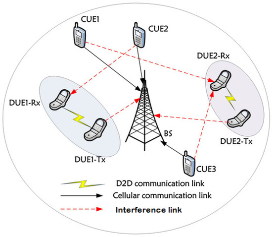
Figure 1. D2D communications—interference challenge.

In this paper, we focus on the power control mechanism using stochastic geometry tools while considering general fading channel conditions. Further, we analyze the energy-harvesting capability in the D2D case. The contributions of this paper are summarized as follows:

• In the context of D2D underlaid communications, we analyze the SINR at the receiver side when the channel fading is modeled as $\kappa$-$\mu$ shadowed. We then derive the CDF of the required transmission power to achieve the target where the SINR is greater than a threshold.
• Based on the general form of CDF, some particular cases of channel fading, especially Nakagami and Rayleigh fading channels, are also derived. We also derive the transmit power distribution in a noiseless environment.
• We consider the case where D2D transmitters are equipped with a radio frequency harvesting system. We assume that the power is gathered from the cellular users’ equipment transmitted energy. Then, we derive the expectation of the harvested energy. In addition, we calculate the expectation of the transmit power of D2D transmitters. Based on this finding, we suggest the probability that a D2D transmitter can achieve its transmission successfully.
• Finally, the accuracy of the analytical results under different fading channel schemes is assessed through an extensive numerical simulation.

The remainder of this paper is structured as follows: In Section 2 we discuss some related works. Section 3 presents the system model for D2D communications under $\kappa$-$\mu$ shadowed fading channels. Section 4 analytically provides the distribution of transmit power and derives some relevant special cases. In Section 5, we present an RF energy-harvesting model based on the cellular ambient RF transmissions. Section 6 provides numerical results for both simulations and analytical derivations. Finally, the Section 7 concludes the paper.

2. Related Work

In order to deal with the interference issue, generally, transmit power control uses channel state information (CSI) between the sender and receiver to meet the required signal-to-noise ratio [12]. In order to model the channel, many recent works use some basic distributions, but the fitting of the shadowed $\kappa$-$\mu$ distribution to experimental data is better than that achieved by the classical distributions previously mentioned. It provides a general multi-path model for a line-of-sight (LOS) propagation scenario controlled by two shape parameters $\kappa$ and $\mu$, in which, the LOS component is subject to shadowing. In addition, some classical fading distributions are included in the shadowed $\kappa$-$\mu$ distribution as particular cases, e.g., one-sided Gaussian, Rayleigh, Nakagami-m, Rician and $\kappa$-$\mu$ [13]. More recently, other generalized fading models are proposed, such as $\alpha$-$\kappa$-$\mu$, $\alpha$-$\eta$-$\mu$ and $\alpha$-$\kappa$-$\mu$ shadowed [14,15].

D2D equipments are battery-powered leading to consider the energy as a main concern for the communication networks. Some literature works have energy management and optimization as the main concern ([16,17,18,19]). Recently, in [20], the authors proposed a technique to handle the battery non-linearity in order to extend the network usage duration.

Another interesting technology that can significantly help in increasing the D2D device lifetime is radio frequency energy harvesting (RF-EH). It is defined as the capability to convert the received RF signals into electricity in order to help the device in its information processing and transmission [21]. This technique is commonly utilized in energy-constrained wireless networks, as they have a limited lifetime that largely confines the network performance. It can be applied in multiple fields, such as wireless sensor networks, wireless body networks and wireless charging systems. In RF-EH, radio signals with frequencies from 3 kHz to 300 GHz are used as a medium to carry energy in an electromagnetic radiation form. The received signal strength decays inversely proportionally to the traveled distance, specifically at 20 dB per decade of the distance [22]. Hence, the RF-EH depends on three main factors: the transmit power, the distance between the energy source and the harvester and the wavelength of the RF signals [23]. It has been shown that it is possible to harvest 3.5 mW of power at a distance of 0.6 m and 1 $\mathsf{\mu }$W at a distance of 11 m using a Powercast RF energy harvester module operating at 915 MHz [24]. RF-EH was discussed in [25] for cognitive radio networks. An RF power conversion circuit extracts DC power from the received RF signals. The circuit is activated only when the received RF power is greater than a predefined threshold, which depends on circuit sensitivity. Similarly, in [26], an energy-harvesting region was considered for relay users, where they harvest ambient RF energy from access points. By considering energy harvesting, the distribution of relays is derived in order to increase the D2D transmission opportunities. Authors in [27] have proposed an IoT energy-harvesting model that does not require battery storage, nor a voltage converter. The implementation tests of the proposed system showed an 8% increase in the amount of harvested power and a 60% increase in the device lifetime. More recently, in [28], the authors conducted experiments with zero energy IoT devices, where the needed power supply was scavenged from the RF signal. In the context of energy harvesting, RF sources can be devised into two categories: dedicated RF sources and ambient ones. Dedicated RF sources use ISM frequency bands. They are used when a more predictable energy supply is needed, but they have some inconveniences, such as generating a high deployment cost, and their power can be limited by federal regulations due to health and safety concerns about RF radiation. On the other side, as the ambient RF sources are not intended specifically for RF energy transfer, they provide free energy [22]. More recently, in [29], authors considered the impact of the RF power density variation on the instantaneous charging capacity of the energy buffer in the RF energy-harvesting system. Although RF-EH has the lowest energy intensity compared to other sources of energy, it has some advantages. In particular, it does not depend on the weather or geographical conditions (unlike solar and wind energy); it can be used in any location where there is ambient RF waves; and it can serve multiple device at the same time [24]. It is important to note that a wireless power transfer can be used for equipments that required an important power supply, as experimented in [30].

In Table 1, we summarize the contribution of the present work as a comparison to the literature review.

Table 1. Contribution of this work related to literature review.

Paper	Cellular/D2D Frequency Band	Channel Fading	Contribution
Sun et al. [31]	Ad hoc networks	Rayleigh	Transmit power CDF
Erturk et al. [32]	different	Rayleigh	Transmit power CDF and SINR
Banagar et al. [33]	same	Rayleigh	Transmit power CDF
Boumaalif et al. [34]	same	Nakagami	Transmit power CDF and device lifetime
Our present work	same	$\kappa$-$\mu$ shadowed	Transmit power CDF and user transmit probability in case of energy harvesting

The list of all of the abbreviations cited in this paper is summarized in the following Table 2:

Table 2. List of abbreviations.

Abbreviation	Signification
D2D	Device-to-Device
CDF	Cumulative Distribution Function
RF-EH	Radio Frequency Energy Harvesting
IoT	Internet of Things
CSI	Channel State Information
LOS	Line-Of-Sight
SINR	Signal to Interference plus Noise Ratio
PPP	Poisson Point Processes
PDF	Probability Density Function
CCDF	Complementary Cumulative Distribution Function
PGFL	Probability Generating Functional

3. System Model

In this work, we considered an underlaid scenario where multiple macro-cellular UEs and D2D users share the same frequency band as depicted in Figure 2. Independent homogeneous Poisson point processes (PPP) ${\mathsf{\Phi }}_C$ and ${\mathsf{\Phi }}_D$ with constant intensity ${\lambda }_C$ and ${\lambda }_D$ were used to model the location of cellular and D2D equipment, respectively. In order to transmit, each UE uses independent and identically distributed (i.i.d.) transmit powers.

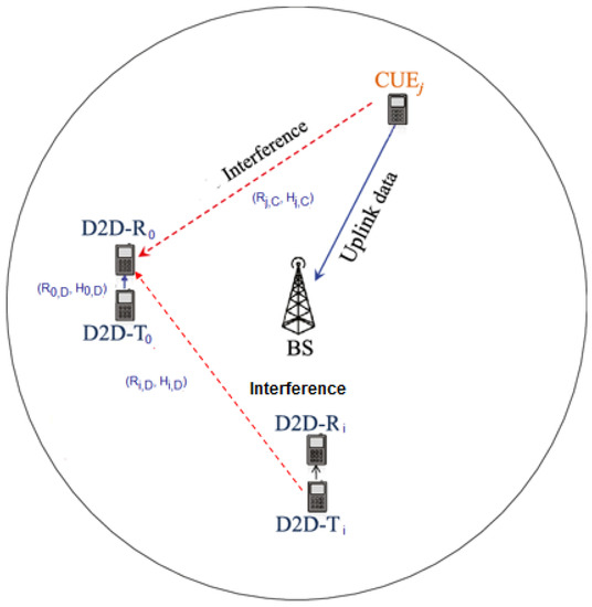
Figure 2. System model.

We assumed that all links are affected by i.i.d. $\kappa$-$\mu$ shadowed fading, and we denoted by H the fading power. For the sake of brevity, we say that: $H\sim S(\beta ,\kappa ,\mu ,m)$, where $\beta =\mathbb{E}\left[H\right]$ is the mean of H, and $\kappa ,\mu ,m$ are the parameters of the $\kappa ,\mu$ shadowed distribution, with the conditions that: $\mu ,m\in \mathbb{N}$, and $\mu \le m$.

With this setting, and from [35], eqn. (4b)], the PDF of H is expressed as:

$$f_H\left(x\right)\approx {\displaystyle \frac{{\omega }^d}{\mathsf{\Gamma }\left(d\right)}}.x^{d-1}.e^{-\omega .x}$$

(1)

with parameters defined as $d={\displaystyle \frac{m\mu {(1+\kappa )}^2}{m+\mu {\kappa }^2+2m\kappa }}$, and $\omega ={\displaystyle \frac{d}{\beta }}$.

In addition, the CCDF of H (from [36], Equation (13)]) is given as:

$${\overline{F}}_H\left(x\right)=\sum _{i=0}^{m-\mu }{b}_i.e^{-c.x}\sum _{j=0}^{m-i-1}\frac{1}{j!}{c}^j.x^j,$$

(2)

with $c={\displaystyle \frac{m\mu (1+\kappa )}{\beta (\mu \kappa +m)}}$, and $b_i={\displaystyle \frac{(m-\mu )!}{i!(m-\mu -i)!}}.{\left({\displaystyle \frac{m}{\mu \kappa +m}}\right)}^i{\left({\displaystyle \frac{\mu \kappa }{\mu \kappa +m}}\right)}^{m-\mu -i}$.

For a transmitter–receiver distance R, the path loss has a standard singular model of $R^{-\alpha }$ with a path-loss exponent $\alpha$ with $2<\alpha <6$.

We supposed that each D2D receiver only connects to the nearest D2D transmitter and that each D2D transmitter communicates with exactly one D2D receiver. This is ensured if the D2D receiver outnumbers the D2D transmitter, if not, some D2D transmitters will have no receiver, and these D2D transmitters will be inactive [32].

Without a loss of generality, we are interested in a typical D2D link where the transmitter is located at the origin $\mathit{O}$, and denote it as subscript 0. Let $P_0$ be the typical D2D transmitter transmit power, $H_0$ be the fading power in the typical D2D communication channel and the distance between the typical D2D transmitter and receiver be $R_0$. Hence, we can express the received power in the typical D2D link as

$$P_r=P_{0,D}.H_{0,D}.R_{0,D}^{-\alpha },$$

(3)

At the typical D2D receiver, the total interference caused by the other D2D transmitters is given as:

$$I_D=\sum _{i\in \{{\varphi }_D\backslash \mathit{O}\}}{P}_{i,D}.H_{i,D}.R_{i,D}^{-\alpha },$$

(4)

and the interference caused by all cellular transmitters is given by the following expression:

$$I_C=\sum _{i\in {\varphi }_C}{P}_{i,C}.H_{i,C}.R_{i,C}^{-\alpha },$$

(5)

where $P_{i,.}$, $H_{i,.}$ and $R_{i,.}$ represent the transmit power, the channel fading power and the locations of the cellular user (subscript C) and D2D users (subscript D), respectively. In the expression of D2D interference $I_D$, we exclude the signal power generated by our D2D typical transmitter. Note that $I_C$ and $I_D$ are independents, as we consider that the transmit power, the fading power and the location of cellular and D2D users are all independent of each other.

In this paper, we focus our study on one macro-cell area, and we consider that the interference from other neighbor cells is negligible. Thus, the $SINR$ at the typical D2D receiver is given by

$$SINR=\frac{P_r}{I_C+I_D+N_0}=\frac{P_{0,D}.H_{0,D}.R_{0,D}^{-\alpha }}{I_C+I_D+N_0}\ge T,$$

(6)

where $N_0$ is the noise power and T is the minimum $SINR$ threshold required for a successful communication between a D2D pair. Table 3 recaps all variables used in our system model:

Table 3. List of variables.

Variable	Signification
${\mathsf{\Phi }}_C$	The location of cellular equipments following independent homogeneous PPP
${\mathsf{\Phi }}_D$	The location of D2D equipments following independent homogeneous PPP
${\lambda }_C$	The intensity of ${\mathsf{\Phi }}_C$
${\lambda }_D$	The intensity of ${\mathsf{\Phi }}_D$
H	The fading power
$f_H(x)$	The PDF of H
${\overline{F}}_H(x)$	The CCDF of H
$P_0$	The typical D2D transmitter transmit power
$H_0$	The fading power in the typical D2D communication channel
$R_0$	The distance between the typical D2D transmitter and receiver
$P_r$	The received power in the typical D2D link
$I_D$	The interference caused by the other D2D transmitters to the typical D2D receiver
$I_C$	The interference caused by all cellular transmitters to the typical D2D receiver
$SINR$	The $SINR$ at the typical D2D receiver
$N_0$	The noise power
T	The minimum $SINR$ threshold

4. CDF of Transmit Power

Theorem 1.

In a D2D-underlaid cellular network with multiple macro-cellular UEs and D2D users, the converged$CDF$ of the transmit power of D2D users, assuming κ-μ shadowed fading channels, is

$$\begin{array}{cc}\hfill \mathbb{P}(P\le p)& =\sum _{i,j}f(i,j).{\int }_0^{\infty }{r}^{1+\alpha j}.e^{-k_1.r^{\alpha }-k_2.r^2}dr\hfill \\ \hfill & +\sum _{i,j,k,l,M}g(i,j,k,l,M).{\int }_0^{\infty }{r}^{1+2l+\alpha (j-k)}.e^{-k_1.r^{\alpha }-k_2.r^2}dr\hfill \\ \hfill & +\sum _{i,j,k,t,l,s,M}h(i,j,k,t,l,s,M){\int }_0^{\infty }{r}^{1+2(l+s)+\alpha (j-k)}.e^{-k_1{r}^{\alpha }-k_2{r}^2}dr\hfill \end{array}$$

(7)

where $k_1$, $k_2$, $f(.)$, $g(.,.)$ and $h(.,.)$ will be detailed by the end of the proof.

Proof. 

The $CDF$ of the D2D transmit power, where it is conditioned on $R_0$ and considering $I=I_C+I_D$, is

$$\begin{array}{cc}\hfill \mathbb{P}(P\le p)& =\mathbb{P}\left(H_0\ge \frac{T.R_0^{\alpha }(I+N_0)}{p}\right)\hfill \\ \hfill & ={\mathbb{E}}_R[\mathbb{P}(H_0\ge \frac{T.R_0^{\alpha }(I+N_0)}{p}|R_0)]\hfill \\ \hfill & ={\mathbb{E}}_R[\sum _{i=0}^{m-\mu }{b}_i.e^{-\frac{cT{R}_0^{\alpha }(I+N_0)}{p}}\sum _{j=0}^{m-i-1}\frac{1}{j!}{c}^j{\left(\frac{T.R_0^{\alpha }(I+N_0)}{p}\right)}^j]\hfill \\ \hfill & =\sum _{i=0}^{m-\mu }{b}_i\sum _{j=0}^{m-i-1}\frac{1}{j!}{\left(\frac{Tc}{p}\right)}^j{\mathbb{E}}_R\left[R_0^{\alpha .j}.e^{-\frac{cT{N}_0}{p}{R}_0^{\alpha }}.{(I+N_0)}^j.e^{-\frac{cT}{p}I.R_0^{\alpha }}\right]\hfill \\ \hfill & =\sum _{i=0}^{m-\mu }{b}_i\sum _{j=0}^{m-i-1}\frac{1}{j!}{\left(\frac{T.c}{p}\right)}^j{\mathbb{E}}_R\left[R_0^{\alpha .j}.e^{-\frac{cT{N}_0}{p}{R}_0^{\alpha }}.{\mathbb{E}}_I[{(I+N_0)}^j.e^{-\frac{cT{R}_0^{\alpha }}{p}I}|R_0]\right]\hfill \\ \hfill & =\sum _{i=0}^{m-\mu }{b}_i\sum _{j=0}^{m-i-1}\frac{1}{j!}{\left(\frac{Tc}{p}\right)}^j\sum _{k=0}^j{C}_j^k.N_0^{j-k}{\mathbb{E}}_R\left[R_0^{\alpha .j}.e^{-\frac{cT{N}_0}{p}{R}_0^{\alpha }}.{\mathbb{E}}_I[I^k.e^{-\frac{cT{R}_0^{\alpha }}{p}I}|R_0]\right]\hfill \end{array}$$

where $C_j^k={\displaystyle \frac{j!}{k!(j-k)!}}$. Separating the terms when $j=0$ and $k=0$ and making some development, we obtained

$$\begin{array}{cc}\hfill \mathbb{P}(P\le p)& =\sum _{i=0}^{m-\mu }{b}_i\sum _{j=0}^{m-i-1}\frac{1}{j!}{\left(\frac{T.c}{p}\right)}^j{N}_0^j{\mathbb{E}}_R\left[R_0^{\alpha .j}.e^{-\frac{c.T.N_0}{p}{R}_0^{\alpha }}.{\mathbb{E}}_I[e^{-\frac{c.T.R_0^{\alpha }}{p}I}|R_0]\right]\hfill \\ \hfill & +\sum _{i=0}^{m-\mu }{b}_i\sum _{j=1}^{m-i-1}\frac{1}{j!}{\left(\frac{T.c}{p}\right)}^j\sum _{k=1}^j{C}_j^k.N_0^{j-k}{\mathbb{E}}_R\left[R_0^{\alpha .j}.e^{-\frac{c.T.N_0}{p}{R}_0^{\alpha }}.{\mathbb{E}}_I[I^k.e^{-\frac{c.T.R_0^{\alpha }}{p}I}|R_0]\right]\hfill \end{array}$$

(8)

Starting with the first expectation over I and putting $s=cT{R}_0^{\alpha }/p$, we obtain

$${\mathbb{E}}_{I_1}={\mathbb{E}}_I[e^{-s.I}]={\mathcal{L}}_I\left(s\right)$$

Since the total interference is: $I=I_D+I_C$ and $I_D$ and $I_C$ are independent, we have

$${\mathbb{E}}_{I_1}={\mathcal{L}}_{I_D}\left(s\right).{\mathcal{L}}_{I_C}\left(s\right)$$

Thus, in the first step, we try to calculate ${\mathcal{L}}_{I_D}\left(s\right)$:

$$\begin{array}{ccc}\hfill {\mathcal{L}}_{I_D}\left(s\right)& =& {\mathbb{E}}_{I_D}[e^{-s.I_D}]\hfill \\ & =& {\mathbb{E}}_{I_D}\left[e^{-s.{\sum }_{i\in \{{\varphi }_D\backslash \mathit{O}\}}{P}_{i,D}.H_{i,D}.R_{i,D}^{-\alpha }}\right]\hfill \\ & =& {\mathbb{E}}_{P,H,\varphi }\left[\prod _{i\in \{{\varphi }_D\backslash \mathit{O}\}}{e}^{-s.P_{i,D}.H_{i,D}.R_{i,D}^{-\alpha }}\right]\hfill \\ & =& {\mathbb{E}}_{\varphi }\left[\prod _{i\in \{{\varphi }_D\backslash \mathit{O}\}}{\mathbb{E}}_P[{\int }_0^{\infty }{e}^{-sy{R}_{i,D}^{-\alpha }{P}_{i,D}}.{\displaystyle \frac{{\omega }^d}{\mathsf{\Gamma }\left(d\right)}}.y^{d-1}{e}^{-\omega y}dy]\right]\hfill \\ & =& {\mathbb{E}}_{\varphi }\left[\prod _{i\in \{{\varphi }_D\backslash \mathit{O}\}}{\mathbb{E}}_P[\frac{{\omega }^d}{{(\omega +s{R}_{i,D}^{-\alpha }{P}_{i,D})}^d}]\right]\hfill \end{array}$$

Based on the probability-generating functional $\left(PGFL\right)$ theorem for $PPP$, and neglecting the small integration from 0 to $R_0$, we obtain:

$$\begin{array}{ccc}\hfill {\mathcal{L}}_{I_D}(s)& =& exp\left[-{\lambda }_D{\int }_{{\mathbb{R}}^2}\left(1-{\mathbb{E}}_P[\frac{{\omega }^d}{{(\omega +s{P}_{i,D}.x^{-\alpha })}^d}]\right)dx\right]\hfill \\ & =& exp\left(-{\lambda }_D.{\mathbb{E}}_P\left[{\int }_{{\mathbb{R}}^2}(1-\frac{{\omega }^d}{{(\omega +s{P}_{i,D}.x^{-\alpha })}^d})dx\right]\right)\hfill \\ & =& exp\left(-{\lambda }_D.{\mathbb{E}}_P\left[2\pi {\int }_0^{\infty }(1-\frac{1}{{(1+\frac{s{P}_{i,D}.r^{-\alpha }}{\omega })}^d})r.dr\right]\right)\hfill \\ & =& exp\left(-{\lambda }_D.{\mathbb{E}}_P\left[\pi {(s{P}_D/\omega )}^{2/\alpha }\frac{\mathsf{\Gamma }(1-\frac{2}{\alpha }).\mathsf{\Gamma }(d+\frac{2}{\alpha })}{\mathsf{\Gamma }(d)}\right]\right)\hfill \\ & =& exp\left(-{\lambda }_D\pi {(\frac{s}{\omega })}^{\frac{2}{\alpha }}.\frac{\mathsf{\Gamma }(1-\frac{2}{\alpha }).\mathsf{\Gamma }(d+\frac{2}{\alpha })}{\mathsf{\Gamma }(d)}{\mathbb{E}}_P\left[P_D^{2/\alpha }\right]\right)\hfill \end{array}$$

By the same way, we obtain for the Laplace transform ${\mathcal{L}}_{I_C}(s)$ with the following result:

$${\mathcal{L}}_{I_C}(s)=exp\left(-{\lambda }_C\pi {(\frac{s}{\omega })}^{\frac{2}{\alpha }}.\frac{\mathsf{\Gamma }(1-\frac{2}{\alpha }).\mathsf{\Gamma }(d+\frac{2}{\alpha })}{\mathsf{\Gamma }(d)}{\mathbb{E}}_P\left[P_C^{2/\alpha }\right]\right)$$

hence, the final expression of ${\mathbb{E}}_{I_1}$ is:

$${\mathbb{E}}_{I_1}=exp\left(-\pi {(\frac{s}{\omega })}^{\frac{2}{\alpha }}.\frac{\mathsf{\Gamma }(1-\frac{2}{\alpha }).\mathsf{\Gamma }(d+\frac{2}{\alpha })}{\mathsf{\Gamma }(d)}({\lambda }_D{\mathbb{E}}_P\left[P_D^{2/\alpha }\right]+{\lambda }_C{\mathbb{E}}_P\left[P_C^{2/\alpha }\right])\right)$$

(9)

now, passing to the second expectation over I in (8), denoted by ${\mathbb{E}}_{I_2}$:

$$\begin{array}{ccc}\hfill {\mathbb{E}}_{I_2}& =& {\mathbb{E}}_I[I^k.e^{-s.I}]\hfill \\ & =& {\mathbb{E}}_I[{(I_D+I_C)}^k.e^{-s(I_D+I_C)}]\hfill \\ & =& {\mathbb{E}}_I[\sum _{t=0}^k{C}_k^t{I}_D^t{I}_C^{k-t}{e}^{-s.I_D}.e^{-s.I_C}]\hfill \\ & =& \sum _{t=0}^k{C}_k^t{\mathbb{E}}_I[(I_D^t.e^{-s.I_D}).(I_C^{k-t}.e^{-s.I_C})]\hfill \\ & =& \sum _{t=0}^k{C}_k^t{\mathbb{E}}_{I_D}[I_D^t.e^{-s.I_D}].{\mathbb{E}}_{I_C}[I_C^{k-t}.e^{-s.I_C}]\hfill \\ & =& {\mathbb{E}}_{I_D}[e^{-s.I_D}].{\mathbb{E}}_{I_C}[I_C^k.e^{-s.I_C}]+{\mathbb{E}}_{I_D}[I_D^k.e^{-s.I_D}].{\mathbb{E}}_{I_C}[e^{-s.I_C}]\hfill \\ & & +\sum _{t=1}^{k-1}{C}_k^t{\mathbb{E}}_{I_D}[I_D^t.e^{-s.I_D}].{\mathbb{E}}_{I_C}[I_C^{k-t}.e^{-s.I_C}]\hfill \end{array}$$

(10)

We note that $C_k^t={\displaystyle \frac{k!}{t!(k-t)!}}$. The last step comes from the fact that the expected value of the product of independent variables is the product of expected values.

Thus, we start by calculating the first term in the last equation, denoted by ${\mathbb{E}}_{I_{2,D}}$. Using Theorem 2 in [37] for $t\in {\mathbb{N}}^{*}$, we have

$$\begin{array}{cc}\hfill {\mathbb{E}}_{I_{2,D}}& ={\mathbb{E}}_{I_D}[I_D^t.e^{-s.I_D}]\hfill \\ \hfill & =exp(-{\lambda }_D{\int }_{{\mathbb{R}}^2\backslash D}(1-{\mathbb{E}}_{H,P}[exp(-s{H}_{i,D}.x^{-\alpha }{P}_{i,D})])dx)\hfill \\ \hfill & .\sum _{l=1}^t\sum _{M\in {\mathbb{N}}^l}\frac{C_M}{l!}\prod _{i=1}^l{\lambda }_D.{\int }_{{\mathbb{R}}^2}{\mathbb{E}}_{H,P}[exp(-s{H}_{i,D}.x^{-\alpha }{P}_{i,D}){(H_{i,D}.x^{-\alpha }{P}_{i,D})}^{m_i}]dx\hfill \end{array}$$

where $C_M={\displaystyle \frac{t!}{{\prod }_{r=1}^l{m}_r!}}$, ${\mathbb{N}}^l$ is the set of vectors M with l natural elements, ${\Vert M\Vert }_1={\sum }_{i=1}^l{m}_i=t$ and D is the disk of origin $O$ and radius $R_0$.

Let us calculate the expressions of ${\mathbb{E}}_{H,P}[1]$ and ${\mathbb{E}}_{H,P}[2]$, related to the expectations given in (11), respectively:

$$\begin{array}{cc}\hfill {\mathbb{E}}_{H,P}[1]& ={\mathbb{E}}_{H,P}[exp(-s{H}_{i,D}{R}^{-\alpha }{P}_{i,D})]\hfill \\ \hfill & =\int \int e^{-s{P}_{i,D}{R}^{-\alpha }.H_{i,D}}.f(H).f(P)dHdP\hfill \\ \hfill & ={\int }_0^{\infty }\left({\int }_0^{\infty }{e}^{-sy{P}_{i,D}{R}^{-\alpha }}\frac{{\omega }^d}{\mathsf{\Gamma }(d)}{y}^{d-1}{e}^{-\omega y}dy\right)f(P)dP\hfill \\ \hfill & ={\mathbb{E}}_P\left[\frac{1}{{(1+\frac{s{R}^{-\alpha }{P}_{i,D}}{\omega })}^d}\right]\hfill \end{array}$$

(11)

The second expectation can be defined as:

$$\begin{array}{cc}\hfill {\mathbb{E}}_{H,P}[2]& ={\mathbb{E}}_{H,P}[exp(-s{H}_{i,D}.R^{-\alpha }{P}_{i,D}).{(H_{i,D}.R^{-\alpha }{P}_{i,D})}^{m_1}]\hfill \\ \hfill & ={\mathbb{E}}_P\left[{\int }_0^{\infty }{e}^{-sy{P}_{i,D}{R}^{-\alpha }}.{(y{P}_{i,D}{R}^{-\alpha })}^{m_i}.\frac{{\omega }^d}{\mathsf{\Gamma }(d)}.y^{d-1}.e^{-\omega y}dy\right]\hfill \\ \hfill & ={\mathbb{E}}_P\left[{(P_{i,D}{R}^{-\alpha })}^{m_i}.\frac{{\omega }^d}{\mathsf{\Gamma }(d)}{\int }_0^{\infty }{y}^{m_i+d-1}.e^{-(s{P}_{i,D}{R}^{-\alpha }+\omega )y}dy\right]\hfill \\ \hfill & ={\mathbb{E}}_P\left[\frac{{\omega }^d.\mathsf{\Gamma }(m_i+d)}{\mathsf{\Gamma }(d)}.\frac{{(P_{i,D}{R}^{-\alpha })}^{m_i}}{{(\omega +s{P}_{i,D}{R}^{-\alpha })}^{m_i+d}}\right]\hfill \end{array}$$

(12)

Based on (11) and (12), the expression of ${\mathbb{E}}_{I_{2,D}}$ is given as:

$$\begin{array}{cc}\hfill {\mathbb{E}}_{I_{2,D}}& =exp\left(-{\lambda }_D{\int }_{{\mathbb{R}}^2\backslash D}(1-{\mathbb{E}}_P[\frac{1}{{(1+\frac{s{x}^{-\alpha }{P}_{i,D}}{\omega })}^d}])dx\right)\hfill \\ \hfill & \sum _{l=1}^t\sum _{M\in {\mathbb{N}}^l}\frac{C_M}{l!}\prod _{i=1}^l{\lambda }_D{\int }_{{\mathbb{R}}^2}{\mathbb{E}}_P\left[\frac{{\omega }^d.\mathsf{\Gamma }(m_i+d)}{\mathsf{\Gamma }(d)}.\frac{{(x^{-\alpha }{P}_{i,D})}^{m_i}}{{(\omega +s{x}^{-\alpha }{P}_{i,D})}^{m_i+d}}\right]dx\hfill \\ \hfill & =exp\left(-{\lambda }_D{\mathbb{E}}_P[{\int }_{{\mathbb{R}}^2\backslash D}(1-\frac{1}{{(1+\frac{s{x}^{-\alpha }{P}_{i,D}}{\omega })}^d})dx]\right)\hfill \\ \hfill & \sum _{l=1}^t\sum _{M\in {\mathbb{N}}^l}\frac{C_M}{l!}\prod _{i=1}^l{\lambda }_D{\mathbb{E}}_P\left[{\int }_{{\mathbb{R}}^2}\frac{{\omega }^d.\mathsf{\Gamma }(m_i+d)}{\mathsf{\Gamma }(d)}.\frac{{(x^{-\alpha }{P}_{i,D})}^{m_i}}{{(\omega +s{x}^{-\alpha }{P}_{i,D})}^{m_i+d}}\right]dx\hfill \end{array}$$

We express both integrals with respect to x:

$$\begin{array}{cc}\hfill J& ={\int }_{{\mathbb{R}}^2\backslash D}\left(1-\frac{1}{{(1+\frac{s{P}_D.x^{-\alpha }}{\omega })}^d}\right)dx\hfill \\ \hfill & \approx 2\pi {\int }_0^{\infty }\left(1-\frac{1}{{(1+\frac{s{P}_D.r^{-\alpha }}{\omega })}^d}\right)r.dr\hfill \\ \hfill & \approx \pi {(\frac{s{P}_D}{\omega })}^{2/\alpha }.{\displaystyle \frac{\mathsf{\Gamma }(1-2/\alpha ).\mathsf{\Gamma }(d+2/\alpha )}{\mathsf{\Gamma }(d)}}\hfill \end{array}$$

The second integral is:

$$\begin{array}{cc}\hfill K& =\frac{{\omega }^d.\mathsf{\Gamma }(m_i+d)}{\mathsf{\Gamma }(d)}{\int }_{{\mathbb{R}}^2}{\displaystyle \frac{{(P_D{x}^{-\alpha })}^{m_i}}{{(\omega +s{P}_D{x}^{-\alpha })}^{d+m_i}}}dx\hfill \\ \hfill & =2\pi \frac{{\omega }^d.\mathsf{\Gamma }(m_i+d)}{\mathsf{\Gamma }(d)}.{\int }_0^{+\infty }{\displaystyle \frac{{(P_D.r^{-\alpha })}^{m_i}}{{(\omega +s{P}_D.r^{-\alpha })}^{d+m_i}}}r.dr\hfill \\ \hfill & =\frac{2\pi }{\alpha .s^{m_i}}.{(\frac{s{P}_D}{\omega })}^{2/\alpha }.\frac{\mathsf{\Gamma }(m_i-\frac{2}{\alpha }).\mathsf{\Gamma }(d+\frac{2}{\alpha })}{\mathsf{\Gamma }(d)}\hfill \end{array}$$

Thus, the final form of ${\mathbb{E}}_{I_{2,D}}$ is given as:

$$\begin{array}{cc}\hfill {\mathbb{E}}_{I_{2,D}}=& exp\left(-{\displaystyle \frac{\pi {\lambda }_D}{\mathsf{\Gamma }(d)}}.{(\frac{s}{\omega })}^{2/\alpha }.\mathsf{\Gamma }(1-\frac{2}{\alpha }).\mathsf{\Gamma }(d+\frac{2}{\alpha }).{\mathbb{E}}_P[P_D^{\frac{2}{\alpha }}]\right)\hfill \\ \hfill & \sum _{l=1}^t\sum _{M\in {\mathbb{N}}^l}{\displaystyle \frac{C_M}{l!}}\prod _{i=1}^l\frac{2\pi {\lambda }_D}{\alpha .s^{m_i}\mathsf{\Gamma }(d)}.{(\frac{s}{\omega })}^{2/\alpha }\mathsf{\Gamma }(d+\frac{2}{\alpha }).\mathsf{\Gamma }(m_i-\frac{2}{\alpha }).{\mathbb{E}}_P[P_D^{\frac{2}{\alpha }}]\hfill \end{array}$$

(13)

Using the same method as done with ${\mathbb{E}}_{I_{2,D}}$, we have:

$$\begin{array}{cc}\hfill {\mathbb{E}}_{I_{2,C}}=& {\mathbb{E}}_{I_C}[I_C^{k-t}.e^{-s.I_C}]\hfill \\ \hfill =& exp\left(-{\displaystyle \frac{\pi {\lambda }_C}{\mathsf{\Gamma }(d)}}.{(\frac{s}{\omega })}^{2/\alpha }.\mathsf{\Gamma }(1-\frac{2}{\alpha }).\mathsf{\Gamma }(d+\frac{2}{\alpha }).{\mathbb{E}}_P[P_C^{\frac{2}{\alpha }}]\right)\hfill \\ \hfill & \sum _{l=1}^{k-t}\sum _{M\in {\mathbb{N}}^l}{\displaystyle \frac{C_M}{l!}}\prod _{i=1}^l\frac{2\pi {\lambda }_C}{\alpha .s^{m_i}\mathsf{\Gamma }(d)}.{(\frac{s}{\omega })}^{2/\alpha }\mathsf{\Gamma }(d+\frac{2}{\alpha }).\mathsf{\Gamma }(m_i-\frac{2}{\alpha }).{\mathbb{E}}_P[P_C^{\frac{2}{\alpha }}]\hfill \end{array}$$

(14)

Now, we can calculate the total expression of ${\mathbb{E}}_{I_2}$ based on (13), (14) and (10):

$$\begin{array}{cc}\hfill {\mathbb{E}}_{I_2}=& exp\left(-{\displaystyle \frac{\pi }{\mathsf{\Gamma }(d)}}.{(\frac{s}{\omega })}^{2/\alpha }.\mathsf{\Gamma }(1-\frac{2}{\alpha }).\mathsf{\Gamma }(d+\frac{2}{\alpha })({\lambda }_D.E_D+{\lambda }_C.E_C)\right)\hfill \\ \hfill & .[\sum _{l=1}^k\sum _{M\in {\mathbb{N}}^l}{\displaystyle \frac{C_M}{l!}}\prod _{i=1}^l\frac{2\pi }{\alpha .s^{m_i}\mathsf{\Gamma }(d)}.{(\frac{s}{\omega })}^{2/\alpha }\mathsf{\Gamma }(d+\frac{2}{\alpha }).\mathsf{\Gamma }(m_i-\frac{2}{\alpha })({\lambda }_D{E}_D+{\lambda }_C{E}_C)\hfill \\ \hfill & +\sum _{t=1}^{k-1}{C}_k^t\left(\sum _{l=1}^t\sum _{M\in {\mathbb{N}}^l}{\displaystyle \frac{C_M}{l!}}\prod _{i=1}^l\frac{2\pi }{\alpha .s^{m_i}\mathsf{\Gamma }(d)}.{(\frac{s}{\omega })}^{2/\alpha }\mathsf{\Gamma }(d+\frac{2}{\alpha }).\mathsf{\Gamma }(m_i-\frac{2}{\alpha }){\lambda }_D{E}_D\right)\hfill \\ \hfill & \left(\sum _{l=1}^{k-t}\sum _{M\in {\mathbb{N}}^l}{\displaystyle \frac{C_M}{l!}}\prod _{i=1}^l\frac{2\pi }{\alpha .s^{m_i}\mathsf{\Gamma }(d)}.{(\frac{s}{\omega })}^{2/\alpha }\mathsf{\Gamma }(d+\frac{2}{\alpha })\mathsf{\Gamma }(m_i-\frac{2}{\alpha }){\lambda }_C{E}_C\right)]\hfill \end{array}$$

(15)

where $E_D={\mathbb{E}}_P[P_D^{\frac{2}{\alpha }}]$ and $E_C={\mathbb{E}}_P[P_C^{\frac{2}{\alpha }}]$.

We can then have the expression of our $CDF$ using the $PDF$ of $R_0$ expressed in [38]: $f_{R_0}(r)=2\pi {\lambda }_{D}r.e^{-\pi {\lambda }_D.r^2}$.

Thus, (8) becomes:

$$\begin{array}{cc}\hfill \mathbb{P}(P\le p)=& \sum _{i=0}^{m-\mu }{b}_i\sum _{j=0}^{m-i-1}\frac{1}{j!}{(\frac{T.c}{p})}^j.N_0^j{\int }_0^{\infty }2\pi \lambda r.e^{-\pi \lambda r^2}{r}^{\alpha j}\hfill \\ \hfill & .e^{-\frac{c.T.N_0}{p}{r}^{\alpha }}.e^{-\frac{\pi }{\mathsf{\Gamma }(d)}{(\frac{cT}{\omega p})}^{\frac{2}{\alpha }}.\mathsf{\Gamma }(1-\frac{2}{\alpha })\mathsf{\Gamma }(d+\frac{2}{\alpha })({\lambda }_D{E}_D+{\lambda }_C{E}_C)r^2}dr\hfill \\ \hfill & +\sum _{i=0}^{m-\mu }{b}_i\sum _{j=1}^{m-i-1}\frac{1}{j!}{(\frac{T.c}{p})}^j.\sum _{k=1}^j{C}_j^k.N_0^{j-k}{\int }_0^{\infty }2\pi \lambda r.e^{-\pi \lambda r^2}{r}^{\alpha j}\hfill \\ \hfill & .e^{-\frac{c.T.N_0}{p}{r}^{\alpha }}.e^{-\frac{\pi }{\mathsf{\Gamma }(d)}{(\frac{cT}{\omega p})}^{\frac{2}{\alpha }}.\mathsf{\Gamma }(1-\frac{2}{\alpha })\mathsf{\Gamma }(d+\frac{2}{\alpha }).({\lambda }_D{E}_D+{\lambda }_C{E}_C).r^2}\hfill \\ \hfill & \sum _{l=1}^k\sum _{M\in {\mathbb{N}}^l}{\displaystyle \frac{C_M}{l!}}\prod _{i=1}^l\frac{2\pi }{\alpha \mathsf{\Gamma }(d)}{(\frac{1}{\omega })}^{\frac{2}{\alpha }}{(\frac{cT}{p})}^{\frac{2}{\alpha }-m_i}\mathsf{\Gamma }(d+\frac{2}{\alpha }).\mathsf{\Gamma }(m_i-\frac{2}{\alpha })({\lambda }_D{E}_D+{\lambda }_C{E}_C)r^{2-\alpha m_i}\hfill \\ \hfill & +\sum _{i=0}^{m-\mu }{b}_i\sum _{j=1}^{m-i-1}\frac{1}{j!}{(\frac{T.c}{p})}^j.\sum _{k=1}^j{C}_j^k.N_0^{j-k}{\int }_0^{\infty }2\pi \lambda r.e^{-\pi \lambda r^2}{r}^{\alpha j}\hfill \\ \hfill & .e^{-\frac{c.T.N_0}{p}{r}^{\alpha }}.e^{-\frac{\pi }{\mathsf{\Gamma }(d)}{(\frac{cT}{\omega p})}^{\frac{2}{\alpha }}.\mathsf{\Gamma }(1-\frac{2}{\alpha })\mathsf{\Gamma }(d+\frac{2}{\alpha }).({\lambda }_D{E}_D+{\lambda }_C{E}_C)r^2}\hfill \\ \hfill & \sum _{t=1}^{k-1}{C}_k^t\left(\sum _{l=1}^t\sum _{M\in {\mathbb{N}}^l}{\displaystyle \frac{C_M}{l!}}\prod _{i=1}^l\frac{2\pi }{\alpha \mathsf{\Gamma }(d)}.{(\frac{1}{\omega })}^{2/\alpha }{(\frac{cT}{p})}^{2/\alpha -m_i}\mathsf{\Gamma }(d+\frac{2}{\alpha }).\mathsf{\Gamma }(m_i-\frac{2}{\alpha }){\lambda }_D{E}_D{r}^{2-\alpha m_i}\right)\hfill \\ \hfill & \left(\sum _{l=1}^{k-t}\sum _{M\in {\mathbb{N}}^l}{\displaystyle \frac{C_M}{l!}}\prod _{i=1}^l\frac{2\pi }{\alpha \mathsf{\Gamma }(d)}{(\frac{1}{\omega })}^{\frac{2}{\alpha }}{(\frac{cT}{p})}^{\frac{2}{\alpha }-m_i}\mathsf{\Gamma }(d+\frac{2}{\alpha })\mathsf{\Gamma }(m_i-\frac{2}{\alpha }){\lambda }_C{E}_C{r}^{2-\alpha m_i}\right)dr\hfill \end{array}$$

(16)

Finally, the transmit power CDF is expressed as follows:

$$\begin{array}{cc}\hfill \mathbb{P}(P\le p)=& \sum _{i,j}f(i,j){\int }_0^{\infty }{r}^{1+\alpha j}{e}^{-k_1{r}^{\alpha }-k_2{r}^2}dr\hfill \\ \hfill & +\sum _{i,j,k,l,M}g(i,j,k,l,M){\int }_0^{\infty }{r}^{1+2l+\alpha (j-k)}{e}^{-k_1{r}^{\alpha }-k_2{r}^2}dr\hfill \\ \hfill & +\sum _{i,j,k,t,l,M}h(i,j,k,t,l,M){\int }_0^{\infty }{r}^{1+2(l+s)+\alpha (j-k)}{e}^{-k_1{r}^{\alpha }-k_2{r}^2}dr\hfill \end{array}$$

(17)

where $k_1=\frac{cT{N}_0}{p}$, $k_2=\pi {\lambda }_D+\pi {(\frac{cT}{\omega p})}^{2/\alpha }.\frac{\mathsf{\Gamma }(1-\frac{2}{\alpha }).\mathsf{\Gamma }(d+\frac{2}{\alpha })}{\mathsf{\Gamma }(d)}({\lambda }_D{E}_D+{\lambda }_C{E}_C).$

Therefore, we have the first integral multiplier $\sum _{i,j}f(i,j)={\displaystyle \sum _{i=0}^{m-\mu }}{b}_i{\displaystyle \sum _{j=0}^{m-i-1}}\frac{2\pi {\lambda }_D}{j!}{(\frac{Tc}{p})}^j.N_0^j$, the second $\begin{array}{l}{\sum }_{i,j,k,l,M}g(i,j,k,l,M)={\displaystyle \sum _{i=0}^{m-\mu }}{b}_i{\displaystyle \sum _{j=1}^{m-i-1}}\frac{2\pi {\lambda }_D}{j!}{(\frac{Tc}{p})}^j{\displaystyle \sum _{k=1}^j}{C}_j^k{N}_0^{j-k}\\ {\displaystyle \sum _{l=1}^k}{\displaystyle \sum _{M\in {\mathbb{N}}^l}}{\displaystyle \frac{C_M}{l!}}{\prod }_{i=1}^l\frac{2\pi }{\alpha \mathsf{\Gamma }(d)}.{(\frac{1}{\omega })}^{2/\alpha }{(\frac{cT}{p})}^{2/\alpha -m_i}\mathsf{\Gamma }(m_i-\frac{2}{\alpha })\mathsf{\Gamma }(d+\frac{2}{\alpha })({\lambda }_D{E}_D+{\lambda }_C{E}_C),\end{array}$ and the last integral multiplier$\begin{array}{l}{\sum }_{i,j,k,t,l,M}h(i,j,k,t,l,M)={\displaystyle \sum _{i=0}^{m-\mu }}{b}_i{\displaystyle \sum _{j=1}^{m-i-1}}\frac{2\pi {\lambda }_D}{j!}{(\frac{Tc}{p})}^j{\displaystyle \sum _{k=1}^j}{C}_j^k{N}_0^{j-k}{\displaystyle \sum _{t=1}^{k-1}}{C}_k^t{\displaystyle \sum _{l=1}^t}{\displaystyle \sum _{s=1}^{k-t}}{({\lambda }_D{E}_D)}^l{({\lambda }_C{E}_C)}^s\\ ({\displaystyle \sum _{M\in {\mathbb{N}}^l}}{\displaystyle \frac{C_M}{l!}}{\prod }_{i=1}^l\frac{2\pi }{\alpha \mathsf{\Gamma }(d)}.{(\frac{1}{\omega })}^{2/\alpha }{(\frac{cT}{p})}^{2/\alpha -m_i}\mathsf{\Gamma }(m_i-\frac{2}{\alpha })\mathsf{\Gamma }(d+\frac{2}{\alpha }))\\ ({\displaystyle \sum _{M\in {\mathbb{N}}^s}}{\displaystyle \frac{C_M}{s!}}{\prod }_{i=1}^s\frac{2\pi }{\alpha \mathsf{\Gamma }(d)}.{(\frac{1}{\omega })}^{2/\alpha }{(\frac{cT}{p})}^{2/\alpha -m_i}\mathsf{\Gamma }(m_i-\frac{2}{\alpha })\mathsf{\Gamma }(d+\frac{2}{\alpha }))\end{array}$

• There is a circularity in our CDF, in which, $E_D$ depends on the PDF of $P_D$. Thus, by differentiating (17) and making some variables change, we obtain:

$$\begin{array}{cc}\hfill E_D& =\sum _{i,j}{f}^{\prime }(i,j){\int }_0^{\infty }\frac{1}{2A_2^2}\left(-j.x^{j-1-\frac{2}{\alpha }}+A_1{x}^{j-\frac{2}{\alpha }}+{\displaystyle \frac{2A_3}{\alpha }}{x}^{j-1}+{\displaystyle \frac{2A_4}{\alpha }}{E}_D{x}^{j-1}\right).e^{-A_{1}x-A_3{x}^{2/\alpha }-A_4.E_D.x^{\frac{2}{\alpha }}}dx\hfill \\ \hfill & +\frac{1}{2A_2^2}\sum _{i,j,k,l}{g}^{\prime }(i,j,k,l){\int }_0^{\infty }\left[(k-\frac{2l}{\alpha }-j)x^{-1}+A_1+{\displaystyle \frac{2}{\alpha }}{A}_3{x}^{\frac{2}{\alpha }-1}+{\displaystyle \frac{2}{\alpha }}{A}_4.E_D.x^{\frac{2}{\alpha }-1}\right]\hfill \\ \hfill & .x^{\frac{2l}{\alpha }+j-\frac{2}{\alpha }-k}.e^{-A_{1}x-A_3{x}^{2/\alpha }-A_4.E_D.x^{\frac{2}{\alpha }}}dx\hfill \\ \hfill & +\frac{1}{2A_2^2}\sum _{i,j,k,l}{h}^{\prime }(i,j,k,l){\int }_0^{\infty }\left[(k-\frac{2(l+s)}{\alpha }-j)x^{-1}+A_1+{\displaystyle \frac{2}{\alpha }}{A}_3{x}^{\frac{2}{\alpha }-1}+{\displaystyle \frac{2}{\alpha }}{A}_4.E_D.x^{\frac{2}{\alpha }-1}\right]\hfill \\ \hfill & .x^{\frac{2(l+s)}{\alpha }+j-\frac{2}{\alpha }-k}.e^{-A_{1}x-A_3{x}^{2/\alpha }-A_4.E_D.x^{\frac{2}{\alpha }}}dx\hfill \end{array}$$

(18)

with: $A_1=cT{N}_0;A_2=\pi {\lambda }_D;$ $A_3=\pi {(\frac{cT}{\omega })}^{\frac{2}{\alpha }}.\frac{\mathsf{\Gamma }(1-\frac{2}{\alpha }).\mathsf{\Gamma }(d+\frac{2}{\alpha })}{\mathsf{\Gamma }(d)}{\lambda }_C{E}_C;$ $A_4=\pi {(\frac{cT}{\omega })}^{\frac{2}{\alpha }}$$.\frac{\mathsf{\Gamma }(1-\frac{2}{\alpha }).\mathsf{\Gamma }(d+\frac{2}{\alpha })}{\mathsf{\Gamma }(d)}{\lambda }_D;$

$\begin{array}{l}{\displaystyle \sum _{i,j}}{f}^{\prime }(i,j)={\sum }_{i=0}^{m-\mu }{b}_i{\sum }_{j=0}^{m-i-1}\frac{2\pi {\lambda }_D}{j!}{(T.c)}^j.N_0^j;\\ {\displaystyle \sum _{i,j,k,l}}{g}^{\prime }(i,j,k,l)={\displaystyle \sum _{i=0}^{m-\mu }}{b}_i{\displaystyle \sum _{j=1}^{m-i-1}}\frac{2\pi {\lambda }_D}{j!}{(Tc)}^j{\displaystyle \sum _{k=1}^j}{C}_j^k{N}_0^{j-k}{\displaystyle \sum _{l=1}^k}{\displaystyle \sum _{M\in {\mathbb{N}}^l}}{\displaystyle \frac{C_M}{l!}}{\prod }_{i=1}^l\\ \frac{2\pi }{\alpha \mathsf{\Gamma }(d)}.{(\frac{1}{\omega })}^{2/\alpha }{(cT)}^{2/\alpha -m_i}\mathsf{\Gamma }(m_i-\frac{2}{\alpha })\mathsf{\Gamma }(d+\frac{2}{\alpha })({\lambda }_D{E}_D+{\lambda }_C{E}_C),\end{array}$

$\begin{array}{l}{\displaystyle \sum _{i,j,k,l}}{h}^{\prime }(i,j,k,l)={\displaystyle \sum _{i=0}^{m-\mu }}{b}_i{\displaystyle \sum _{j=1}^{m-i-1}}\frac{2\pi {\lambda }_D}{j!}{(Tc)}^j{\displaystyle \sum _{k=1}^j}{C}_j^k{N}_0^{j-k}{\displaystyle \sum _{t=1}^{k-1}}{C}_k^t{\displaystyle \sum _{l=1}^t}{\displaystyle \sum _{s=1}^{k-t}}{({\lambda }_D{E}_D)}^l{({\lambda }_C{E}_C)}^s\\ ({\displaystyle \sum _{M\in {\mathbb{N}}^l}}{\displaystyle \frac{C_M}{l!}}{\prod }_{i=1}^l\frac{2\pi }{\alpha \mathsf{\Gamma }(d)}.{(\frac{1}{\omega })}^{2/\alpha }{(cT)}^{2/\alpha -m_i}\mathsf{\Gamma }(m_i-\frac{2}{\alpha })\mathsf{\Gamma }(d+\frac{2}{\alpha }))\\ ({\displaystyle \sum _{M\in {\mathbb{N}}^s}}{\displaystyle \frac{C_M}{s!}}{\prod }_{i=1}^s\frac{2\pi }{\alpha \mathsf{\Gamma }(d)}.{(\frac{1}{\omega })}^{2/\alpha }{(cT)}^{2/\alpha -m_i}\mathsf{\Gamma }(m_i-\frac{2}{\alpha })\mathsf{\Gamma }(d+\frac{2}{\alpha }))\end{array}$

This result is still difficult to solve analytically, so we should use numerical techniques to solve it.

The convergence of our power distribution is obtained with the Foschini–Miljanic algorithm described in Section 5.

• Based on Table I in [39], we can obtain many distributions. As the $\kappa$-$\mu$ distribution is a special case of a $\kappa$-$\mu$ shadowed distribution (when $\mu \le m$), we can easily express our CDF in the case of the $\kappa$-$\mu$ fading environment by putting $m\to \infty$. We will highlight other special cases in the following corollaries, as they have more closed forms.

□

Corollary 1.

In the Nakagami fading case, the CDF is

$$\begin{array}{cc}\hfill \mathbb{P}(P\le p)=& \sum _{j}f(j){\int }_0^{\infty }{r}^{1+\alpha j}{e}^{-k_1{r}^{\alpha }-k_2{r}^2}dr\hfill \\ \hfill & +\sum _{j,k,l,M}g(j,k,l,M){\int }_0^{\infty }{r}^{1+2l+\alpha (j-k)}{e}^{-k_1{r}^{\alpha }-k_2{r}^2}dr\hfill \\ \hfill & +\sum _{j,k,t,l,s,M}h(j,k,t,l,s,M){\int }_0^{\infty }{r}^{1+2(l+s)+\alpha (j-k)}{e}^{-k_1{r}^{\alpha }-k_2{r}^2}dr\hfill \end{array}$$

(19)

The CDF has the same general form, but the external parameters are more simplified:

$k_1=\frac{T.N_0}{\theta .p},$ 

$k_2=\pi {\lambda }_D+\pi {(\frac{T}{p})}^{2/\alpha }.\frac{\mathsf{\Gamma }(1-2/\alpha ).\mathsf{\Gamma }(n+2/\alpha )}{(n-1)!}({\lambda }_D{E}_D+{\lambda }_C{E}_C),$

$\hspace{1em}\hspace{1em}{\sum }_{j}f(j)={\displaystyle \sum _{j=0}^{n-1}}\frac{2\pi {\lambda }_D}{j!}{(\frac{T}{p\theta })}^j.N_0^j$,

$\begin{array}{l}{\sum }_{j,k,l,M}g(j,k,l,M)={\displaystyle \sum _{j=1}^{n-1}}\frac{2\pi {\lambda }_D}{j!}{(\frac{T}{p\theta })}^j{\displaystyle \sum _{k=1}^j}{C}_j^k{N}_0^{j-k}{\displaystyle \sum _{l=1}^k}{\displaystyle \sum _{M\in {\mathbb{N}}^l}}{\displaystyle \frac{C_M}{l!}}{\prod }_{i=1}^l\frac{2\pi {\theta }^{2/\alpha }}{\alpha (n-1)!}{(\frac{T}{p\theta })}^{2/\alpha -m_i}\mathsf{\Gamma }(m_i-\frac{2}{\alpha })\\ \mathsf{\Gamma }(n+\frac{2}{\alpha })({\lambda }_D{E}_D+{\lambda }_C{E}_C),\end{array}$

$\begin{array}{l}{\displaystyle \sum _{j,k,t,l,s,M}}h(j,k,t,l,s,M)={\displaystyle \sum _{j=1}^{n-1}}\frac{2\pi {\lambda }_D}{j!}{(\frac{T}{p\theta })}^j{\displaystyle \sum _{k=1}^j}{C}_j^k{N}_0^{j-k}{\displaystyle \sum _{t=1}^{k-1}}{C}_k^t{\displaystyle \sum _{l=1}^t}{\displaystyle \sum _{s=1}^{k-t}}{({\lambda }_D{E}_D)}^l{({\lambda }_C{E}_C)}^s\\ ({\displaystyle \sum _{M\in {\mathbb{N}}^l}}{\displaystyle \frac{C_M}{l!}}{\prod }_{i=1}^l\frac{2\pi {\theta }^{2/\alpha }}{\alpha (n-1)!}{(\frac{T}{p\theta })}^{2/\alpha -m_i}\mathsf{\Gamma }(m_i-\frac{2}{\alpha })\mathsf{\Gamma }(n+\frac{2}{\alpha }))\\ .({\displaystyle \sum _{M\in {\mathbb{N}}^s}}{\displaystyle \frac{C_M}{s!}}{\prod }_{i=1}^s\frac{2\pi {\theta }^{2/\alpha }}{\alpha (n-1)!}{(\frac{T}{p\theta })}^{2/\alpha -m_i}\mathsf{\Gamma }(m_i-\frac{2}{\alpha })\mathsf{\Gamma }(n+\frac{2}{\alpha }))\end{array}$

This result is found by putting $\kappa =0$, $\mu =m=n$ and $\beta =n\theta$, where n is the shape parameter and $\theta$ is the scale parameter of gamma distribution.

Corollary 2.

In the case of Rayleigh fading, the CDF can be written as

$$\begin{array}{c}\hfill \mathbb{P}(P\le p)={\int }_0^{\infty }{e}^{-k_1{r}^{\alpha /2}-k_{2}r}dr\end{array}$$

(20)

with $k_1=\frac{T.N_0}{\sigma p{(\pi {\lambda }_D)}^{\alpha /2}}$, $k_2=1+\frac{1}{sinc(2/\alpha )}{(\frac{T}{p})}^{\frac{2}{\alpha }}(E_D+\frac{{\lambda }_C}{{\lambda }_D}{E}_C)$

This result is found by putting $\kappa =0$, $\mu =m=1$ and $\beta =\sigma$, where $\sigma$ is the mean of $exp(1/\sigma )$ distribution.

Corollary 3.

In an interference-limited scenario, i.e $N_0\to 0$, the $CDF$ of the $D2D$ transmit power in the Rayleigh environment is simplified to

$$\begin{array}{c}\hfill \mathbb{P}(P\le p)=\frac{1}{1+{(\frac{T}{p})}^{\frac{2}{\alpha }}\frac{1}{sinc(2/\alpha )}(E_D+\frac{{\lambda }_C}{{\lambda }_D}{E}_C)}\end{array}$$

(21)

5. RF Energy-Harvesting Model

In our model, we considered RF energy harvesting for D2D users, where the locations of cellular transmitters contribute to the aggregate RF energy at the D2D harvester. We focused on energy harvesting for D2D users rather than cellular users, since the D2D transmitter requires much less power to communicate over short distances [40]. In addition, similar to [26], we assumed that D2D users cannot simultaneously transmit and harvest RF energy. This is due to the fact that the device can have only one antenna that can be switched between the transmit/receive mode and harvesting mode.

5.1. Expected RF Energy Harvesting Rate

Theorem 2.

The expected RF energy-harvesting rate in the case of Rayleigh fading with mean σ is given as

$$\eta =\frac{2\pi \tau {\nu }_e\sigma {\lambda }_C{E}_C^{\alpha /2}}{(\alpha -2)R_0^{\alpha -2}},$$

(22)

where τ represents the fraction of the time period where the device harvests the RF energy—that is,$0<\tau \le 1$—${\nu }_e$ is the RF energy conversion efficiency and $E_C=\mathbb{E}[P_C^{2/\alpha }]$.

Proof. 

The energy is harvested from the interferences in the $\tau$ product time frame. Let $\mathbb{E}[I_C]$ be the expectation of the interferences

$$\begin{array}{ccc}\hfill \mathbb{E}[I_C]& =& \mathbb{E}\left[\sum _{i\in \left\{{\varphi }_C\right\}}\sigma .R_{i,C}^{-\alpha }\mathbb{E}[P_C]\right]\hfill \\ & =& \sum _{i\in \left\{{\varphi }_C\right\}}\mathbb{E}\left[\sigma .R_{i,C}^{-\alpha }\mathbb{E}[P_C]\right]\hfill \\ & =& \sigma .\mathbb{E}[P_C]\sum _{i\in \left\{{\varphi }_C\right\}}{\mathbb{E}}_{{\varphi }_C}[R_{i,C}^{-\alpha }]\hfill \\ & =& \sigma .\mathbb{E}[P_C]{\mathbb{E}}_{{\varphi }_C}[\sum _{i\in \left\{{\varphi }_C\right\}}{R}_{i,C}^{-\alpha }]\hfill \\ & \stackrel{(a)}{=}& \sigma .\mathbb{E}[P_C]{\lambda }_C{\int }_{{\mathbb{R}}^2}{x}^{-\alpha }dx\hfill \\ & =& 2\pi \sigma .\mathbb{E}[P_C]{\lambda }_C{\int }_0^{\infty }{r}^{1-\alpha }dr\hfill \end{array}$$

(23)

where $(a)$ follows from Campbell’s theorem. The last integral diverges due to the lower bound, which is a consequence of the path loss law and the property of PPP where nodes can be arbitrarily close. However, in a real scenario, the interferers cannot coexist in the same location as the typical user. Thus, a small distance $R_0$ from the closest interferer is considered. In addition, assuming that the cellular transmit power is constant, then $\mathbb{E}[P_C]=E_C^{\alpha /2}$. Substituting in (23) concludes the proof. □

Corollary 4.

In the case of a relatively lossy environment ($\alpha =4$), the energy harvesting rate is expressed as

$$\eta =\pi \tau {\nu }_e\sigma {\lambda }_C{(\frac{E_C}{R_0})}^2,$$

(24)

5.2. Energy Utilization Rate

In the case of Rayleigh fading and a noiseless scenario, we express the D2D transmit power expectation as follows:

Lemma 1.

$$\mathbb{E}[P_D]=P_{max}.{}_2{F}_1(1,\frac{\alpha }{2};\frac{\alpha }{2}+1;-\frac{P_{max}^{2/\alpha }}{\kappa })$$

(25)

where $\kappa ={(T)}^{2/\alpha }\frac{1}{sinc(2/\alpha )}(E_D+\frac{{\lambda }_c}{{\lambda }_D}{E}_C)$, $E_D=\kappa [ln(1+\frac{P_{max}^{2/\alpha }}{\kappa })-\frac{P_{max}^{2/\alpha }}{\kappa +P_{max}^{2/\alpha }}]$and${}_2{F}_1(.)$is the hypergeometric function.

Proof. 

Based on the transmit power limitation, we can rewrite the $CDF$ of the D2D transmit power in the case of noiseless communication given in [33] as:

$$\mathbb{P}(P_D\le p)=\left\{\begin{array}{cc}\frac{1}{1+{(\frac{{\beta }_D}{p})}^{2/\alpha }\frac{1}{sinc(2/\alpha )}(E_D+\frac{{\lambda }_c}{{\lambda }_D}{E}_C)},\hfill & if p\le P_{max}\hfill \\ 1,\hfill & if p>P_{max}\hfill \end{array}\right.$$

(26)

Knowing that $\mathbb{E}[P_D]={\int }_0^{\infty }(1-CDF(x))dx$, we can easily obtain the result. □

In the case of $\alpha =4$, $\mathbb{E}[P_D]$ is simplified as in Lemma 2:

Lemma 2.

$$\mathbb{E}[P_D]=2{\kappa }^2\left[\frac{P_{max}^{1/2}}{\kappa }-ln(\frac{P_{max}^{1/2}}{\kappa }+1)\right]$$

(27)

where $\kappa =\sqrt{T}\frac{\pi }{2}(E_D+\frac{{\lambda }_C}{{\lambda }_D}{E}_C)$ and $E_D=\kappa [ln(1+\frac{P_{max}^{1/2}}{\kappa })-\frac{P_{max}^{1/2}}{\kappa +P_{max}^{1/2}}]$

In order to solve the equation of $\kappa$, we used the Matlab tool “fsolve”, which uses the trust region dogleg algorithm [41].

We already supposed that the device harvests the energy within a $\tau$ fraction of time, and transmits during $1-\tau$. Assuming that the major energy consumption is due to the transmission operation, we obtain the following result.

Theorem 3.

The energy utilization rate in a noiseless scenario and relatively lossy environment ($\alpha =4$) can be expressed as

$$\nu =2(1-\tau ){\kappa }^2\left[\frac{P_{max}^{1/2}}{\kappa }-ln(\frac{P_{max}^{1/2}}{\kappa }+1)\right]$$

(28)

5.3. D2D User Transmission Probability

In the case of $\alpha =4$, and knowing that $\rho =min(1,\frac{\eta }{\nu })$ as defined in [21], we have:

$$\rho =min(1,\frac{\pi \tau {\nu }_e\sigma {\lambda }_C{E}_c^2}{2R_0^2(1-\tau ){\kappa }^2\left[\frac{P_{max}^{1/2}}{\kappa }-ln(\frac{P_{max}^{1/2}}{\kappa }+1)\right]}),$$

(29)

6. Numerical Study

This section aims to provide numerical results that validate our finding. We start by presenting the parameters that we used in this assessment. Then, we give the obtained results and provide some interpretations.

6.1. Simulation Parameters

In this work, we considered a hexagonal cell with $R_{cell}=250$ m, in which, all UEs are uniformly and independently distributed, since the PPP is equivalent to the uniform distribution when the nodes number is already known [42]. For our experiments, we worked with the following values of the used parameters: $\kappa =5$, $\mu =2$, $m=6$, $\beta =1$, ${\lambda }_C={10}^{-4}$, ${\lambda }_D=9\times {10}^{-4}$, $N_0=-100$ dBm, $E_C=5\times {10}^{-8}$, $P_{max}=23$ dBm and $T=0$ dB. The transmitter power allocation was performed in a distributed fashion using the Foschini–Miljanic algorithm [43]. It allows transmitters devices to select their transmission power to achieve the SINR threshold at all links in a distributed manner. The $i^{th}$ D2D transmitter calculates its transmit power at $k+1$ time by:

$$P_i(k+1)=(1-\gamma )P_i(k)\left[1+\frac{\gamma }{1-\gamma }\frac{T}{{\beta }_i}\right],$$

(30)

where T is the SINR threshold, ${\beta }_i$ is the actual SINR of the $i^{th}$ D2D link and $\gamma$ is the convergence rate constant. Thus, each device i should have the information about the value of $\gamma$, T and ${\beta }_i$ at each time k to execute the algorithm, which converges when $T={\beta }_i$. We set the convergence rate constant to $\gamma =0.062$.

6.2. Results and Discussions

Figure 3 shows the analytical and simulated transmit power CDF for different values of path loss exponent $\alpha$. For a large value of $\alpha$, the power required of each transmitter, in compensation of the severe channel power attenuation, becomes large. In addition, we can clearly observe that the analytical curves match the simulation ones.

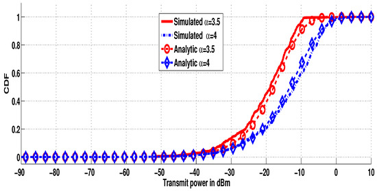
Figure 3. CDF of the transmit power for different values of $\alpha$.

Now, we want to investigate the behavior of our transmit power CDF with regard to different values of the parameter $\kappa$. We used the following simulation parameters: the densities ${\lambda }_C={\lambda }_D={10}^{-4}$, the fading parameters $m=7$, $\mu =1$, $\beta =0.01$, $\alpha =3$, $E_C=5\times {10}^{-8}{W}^{2/3}$ and SINR threshold as $T=0$ dB. Figure 4 shows that, when $\kappa \to 0$ (in the case of Nakagami and Rayleigh fading), i.e the fading power of dominant components becomes negligible, the $CDF$ decreases, i.e., the needed transmit power becomes large. Since increasing $\kappa$ reduces the fading severity, the $CDF$ curves shifts to the left, i.e., the transmit power decreases. In addition, as depicted in this figure, we observe that the transmit power CDF curves become likely identical when the parameter $\kappa$ increases. This result is explained by the fact that, when $\kappa$ increases, the PDF of the fading channel becomes slowly dependent on this parameter. Figure 5 depicts the transmit power CDF for different values of the parameter m. In this experimentation, we worked with the same parameters as above, with $\kappa =10$. We noticed that, for large values of m, the $CDF$ curve shifts to the left side, i.e., for a specified power, the $CDF$ becomes large when m grows, which means that the required transmit power decreases. The reason behind this is that lower values of m means a larger probability of having low $SINR$ values, i.e., a larger fading severity. When m grows, the effect of line of sight (LOS) fluctuation vanishes and the $SINR$ values tend to be more concentrated around its mean value (see Figure 4 in [15]).

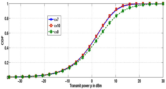
Figure 4. CDF of the transmit power for different values of $\kappa$.

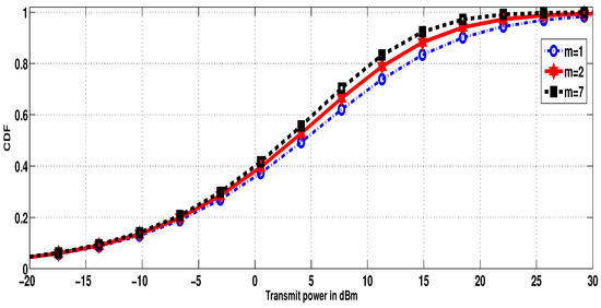
Figure 5. CDF of the transmit power for different values of m.

In the last assessment, we considered the energy harvesting in the transmitter devices. The used parameters were as follows: $\beta =1$, $\alpha =4$, $\tau =0.99$, $E_C=5\times {10}^{-3}{W}^{1/2}$ and $T=10$ dB; the channel power is considered as exponential, with mean $\sigma =1$, as the channel is assumed to be Rayleigh. Figure 6 depicts the variation in the user transmission probability (the parameter $\rho$). As represented, the simulation and analytic results match well. We can observe from this figure that the values of $\rho$ are much less than 1. However, when the cell-users’ density increases, the user transmission probability increases since more cellular equipments are present in the neighborhood of devices; then, they can harvest more energy that they exploit to transmit data. Considering the harvested energy, it appears more interesting to gather energy from the down-link channel rather than the up-link one since the base station can transmit energy with relatively higher power compared to users’ equipment, and then more energy can be harvested.

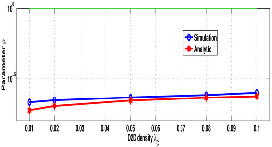
Figure 6. D2D user transmission probability $\rho$ vs. ${\lambda }_C$.

7. Conclusions

In this work, we derived the transmit power distribution of a D2D communication under a $\kappa$-$\mu$ shadowed fading channel using stochastic geometry and considering an underlaid situation of spectrum sharing. Exploiting the finding, we derived the transmit power CDF of some special cases of fading channels—Nakagami and Rayleigh—and we also provided a simple-form CDF in the case of na noiseless environment. Based on the case of Rayleigh fading, we investigated the mechanism of harvesting the RF energy for the device transmitter from its cellular interferers. The simulations showed a good correspondence between the analytical and numerical results, which confirms the validity of our analysis.

References

- Shafique, K.; Khawaja, B.A.; Sabir, F.; Qazi, S.; Mustaqim, M. Internet of Things (IoT) for Next-Generation Smart Systems: A Review of Current Challenges, Future Trends and Prospects for Emerging 5G-IoT Scenarios. IEEE Access 2020, 8, 23022–23040. [Google Scholar] [CrossRef]
- Porambage, P.; Gur, G.; Osorio, D.P.M.; Liyanage, M.; Gurtov, A.; Ylianttila, M. The roadmap to 6G security and privacy. IEEE Open J. Commun. Soc. 2021, 2, 1094–1122. [Google Scholar] [CrossRef]
- Kar, U.N.; Sanyal, D.K. An overview of device-to-device communication in cellular networks. ICT Express 2018, 4, 203–208. [Google Scholar] [CrossRef]
- Alnoman, A.; Anpalagan, A. On D2D communications for public safety applications. In Proceedings of the 2017 IEEE Canada International Humanitarian Technology Conference (IHTC), Toronto, ON, Canada, 21–22 July 2017; pp. 124–127. [Google Scholar] [CrossRef]
- Goratti, L.; Steri, G.; Gomez, K.M.; Baldini, G. Connectivity and security in a D2D communication protocol for public safety applications. In Proceedings of the 2014 11th International Symposium on Wireless Communications Systems (ISWCS), Barcelona, Spain, 26–29 August 2014; pp. 548–552. [Google Scholar] [CrossRef]
- Liu, J.; Kato, N.; Ma, J.; Kadowaki, N. Device-to-Device Communication in LTE-Advanced Networks: A Survey. IEEE Commun. Surv. Tutor. 2014, 17, 1923–1940. [Google Scholar] [CrossRef]
- Han, L.; Zhang, Y.; Zhang, X.; Mu, J. Power Control for Full-Duplex D2D Communications Underlaying Cellular Networks. IEEE Access 2019, 7, 111858–111865. [Google Scholar] [CrossRef]
- Wen, S.; Zhu, X.; Lin, Z.; Zhang, X.; Yang, D. Energy Efficient Power Allocation Schemes for Device-to-Device(D2D) Communication. In Proceedings of the 2013 IEEE 78th Vehicular Technology Conference (VTC Fall), Las Vegas, NV, USA, 2–5 September 2013; pp. 1–5. [Google Scholar] [CrossRef]
- Bulashenko, A.; Piltyay, S.; Demchenko, I. Energy Efficiency of the D2D Direct Connection System in 5G Networks. In Proceedings of the 2020 IEEE International Conference on Problems of Infocommunications. Science and Technology (PIC S&T), Kharkiv, Ukraine, 6–9 October 2020; pp. 537–542. [Google Scholar] [CrossRef]
- Nguyen, K.K.; Duong, T.Q.; Vien, N.A.; Le-Khac, N.-A.; Nguyen, M.-N. Non-Cooperative Energy Efficient Power Allocation Game in D2D Communication: A Multi-Agent Deep Reinforcement Learning Approach. IEEE Access 2019, 7, 100480–100490. [Google Scholar] [CrossRef]
- Doan, T.X.; Hoang, T.M.; Duong, T.Q.; Ngo, H.Q. Energy Harvesting-Based D2D Communications in the Presence of Interference and Ambient RF Sources. IEEE Access 2017, 5, 5224–5234. [Google Scholar] [CrossRef]
- Sun, P.; Shin, K.G.; Zhang, H.; He, L. Transmit Power Control for D2D-Underlaid Cellular Networks Based on Statistical Features. IEEE Trans. Veh. Technol. 2017, 66, 4110–4119. [Google Scholar] [CrossRef]
- Paris, J.F. Statistical Characterization of κ-μ Shadowed Fading. IEEE Trans. Veh. Technol. 2014, 63, 518–526. [Google Scholar] [CrossRef]
- Goswami, A.; Kumar, A. Statistical Characterization and Performance Evaluation of α-η-μ/Inverse Gamma and α-κ-μ/Inverse Gamma Channels. Wirel. Pers. Commun. 2022, 124, 2313–2333. [Google Scholar] [CrossRef]
- Ramirez-Espinosa, P.; Moualeu, J.M.; da Costa, D.B.; Lopez-Martinez, F.J. The α-κ-μ Shadowed Fading Distribution: Statistical Characterization and Applications. In Proceedings of the 2019 IEEE Global Communications Conference (GLOBECOM), Big Island, HI, USA, 9–13 December 2019. [Google Scholar]
- Hunukumbure, M.; Moulsley, T.; Oyawoye, A.; Vadgama, S.; Wilson, M. D2D for energy efficient communications in disaster and emergency situations. In Proceedings of the 2013 21st International Conference on Software, Telecommunications and Computer Networks—(SoftCOM 2013), Split-Primosten, Croatia, 18–20 September 2013; pp. 1–5. [Google Scholar] [CrossRef]
- Anamuro, C.V.; Varsier, N.; Schwoerer, J.; Lagrange, X. Simple modeling of energy consumption for D2D relay mechanism. In Proceedings of the 2018 IEEE Wireless Communications and Networking Conference Workshops (WCNCW), Barcelona, Spain, 15–18 April 2018; pp. 231–236. [Google Scholar] [CrossRef]
- Shang, B.; Zhao, L.; Chen, K.-C.; Chu, X. Energy Efficient D2D-Assisted Offloading with Wireless Power Transfer, GLOBECOM 2017. In Proceedings of the 2017 IEEE Global Communications Conference, Singapore, 4–8 December 2017; pp. 1–6. [Google Scholar] [CrossRef]
- Amiri, M.H.Z.; Nazemi, A.M.; Namazi, M.; Amri, K.J.; Amiri, F.Z. Energy Saving in D2D Cellular 6G Networks. In Proceedings of the 2020 10th International Conference on Computer and Knowledge Engineering (ICCKE), Mashhad, Iran, 29–30 October 2020; pp. 676–682. [Google Scholar] [CrossRef]
- Zytoune, O.; Fouchal, H.; Zeadally, S. A realistic relay selection scheme for cooperative MIMO networks. Ad Hoc Netw. 2022, 124, 102706. [Google Scholar] [CrossRef]
- Atat, R.; Liu, L.; Mastronarde, N.; Yi, Y. Energy Harvesting-Based D2D-Assisted Machine-Type Communications. IEEE Trans. Commun. 2017, 65, 1289–1302. [Google Scholar] [CrossRef]
- Lu, X.; Wang, P.; Niyato, D.; Kim, D.I.; Han, Z. Wireless Networks With RF Energy Harvesting: A Contemporary Survey. IEEE Commun. Surv. Tutor. 2015, 17, 757–789. [Google Scholar] [CrossRef]
- Atat, R.; Chen, H.; Liu, L. Fundamentals of spatial RF energy harvesting for D2D cellular networks. In Proceedings of the 2016 IEEE Global Communications Conference (GLOBECOM), Washington, DC, USA, 4–8 December 2016; pp. 1–6. [Google Scholar]
- Zungeru, A.M.; Ang, L.-M.; Prabaharan, S.R.S.; Seng, K.P. Radio frequency energy harvesting and management for wireless sensor networks. In Green Mobile Devices and Networks; Venkataraman, H., Muntean, G.-M., Eds.; CRC Press: Boca Raton, FL, USA, 2012; Chapter 13; pp. 341–368. [Google Scholar]
- Lee, S.; Zhang, R.; Huang, K. Opportunistic wireless energy harvesting in cognitive radio networks. IEEE Trans. Wirel. Commun. 2013, 12, 4788–4799. [Google Scholar] [CrossRef]
- Yang, H.H.; Lee, J.; Quek, T.Q.S. Heterogeneous cellular network with energy harvesting-based D2D communication. IEEE Trans. Wirel. Commun. 2016, 15, 1406–1419. [Google Scholar] [CrossRef]
- Wang, Y.; Liu, Y.; Wang, C.; Li, Z.; Sheng, X.; Lee, H.G.; Chang, N.; Yang, H. Storage-less and converter-less photovoltaic energy harvesting with maximum power point tracking for internet of things. IEEE Trans. Comput.-Aided Design Integr. Circuits Syst. 2016, 35, 173–186. [Google Scholar] [CrossRef]
- Zeb, H.; Gohar, M.; Ali, M.; Rahman, A.U.; Ahmad, W.; Ghani, A.; Choi, J.-G.; Koh, S.-J. Zero Energy IoT Devices in Smart Cities Using RF Energy Harvesting. Electronics 2023, 12, 148. [Google Scholar] [CrossRef]
- Luo, Y.; Pu, L.; Lei, L. Impact of Varying Radio Power Density on Wireless Communications of RF Energy Harvesting Systems. IEEE Trans. Commun. 2021, 69, 1960–1974. [Google Scholar] [CrossRef]
- Oulcaid, M.; El Fadil, H.; Njili, S.; Zytoune, O.; Bajit, A. Experimental Implementation of a Wireless Communication System for Electric Vehicle WPT Charger. E3S Web Conf. 2022, 351, 01006. [Google Scholar] [CrossRef]
- Sun, C.; Alemseged, Y.D.; Tran, H.N.; Harada, H. Transmit Power Control for Cognitive Radio Over a Rayleigh Fading Channel. IEEE Trans. Veh. Technol. 2010, 59, 1847–1857. [Google Scholar] [CrossRef]
- Erturk, M.C.; Mukherjee, S.; Ishii, H.; Arslan, H. Distributions of Transmit Power and SINR in Device-to-Device Networks. IEEE Commun. Lett. 2013, 17, 273–276. [Google Scholar] [CrossRef]
- Banagar, M.; Maham, B.; Popovski, P.; Pantisano, F. Power Distribution of Device-to-Device Communications in Underlaid Cellular Networks. IEEE Commun. Lett. 2016, 5, 204–207. [Google Scholar] [CrossRef]
- Boumaalif, A.; Zytoune, O. Power Distribution of Device-to-Device Communications Under Nakagami Fading Channel. IEEE Trans. Mob. Comput. 2022, 21, 2158–2167. [Google Scholar] [CrossRef]
- ElHalawany, B.M.; Jameel, F.; da Costa, D.B.; Dias, U.S.; Wu, K. Performance Analysis of Downlink NOMA Systems Over κ-μ Shadowed Fading Channels. IEEE Trans. Veh. Technol. 2020, 69, 1046–1050. [Google Scholar] [CrossRef]
- Lopez-Martinez, F.J.; Paris, J.F.; Romero-Jerez, J.M. The κ-μ Shadowed Fading Model With Integer Fading Parameters. IEEE Trans. Veh. Technol. 2017, 66, 7653–7662. [Google Scholar] [CrossRef]
- Schilcher, U.; Toumpis, S.; Haenggi, M.; Crismani, A.; Brandner, G.; Bettstetter, C. Interference Functionals in Poisson Networks. IEEE Trans. Inf. Theory 2016, 62, 370–383. [Google Scholar] [CrossRef]
- Andrews, J.G.; Baccelli, F.; Ganti, R.K. A Tractable Approach to Coverage and Rate in Cellular Networks. IEEE Trans. Commun. 2011, 59, 3122–3134. [Google Scholar] [CrossRef]
- Moreno-Pozas, L.; Lopez-Martinez, F.J.; Paris, J.F.; Martos-Naya, E. The κ-μ Shadowed Fading Model: Unifying the κ-μ and η-μ Distributions. IEEE Trans. Veh. Technol. 2016, 65, 9630–9641. [Google Scholar] [CrossRef]
- Drayson Technologies. RF Energy Harvesting for the Low Energy Internet of Things. 2015, pp. 1–7. Available online: http://www.getfreevolt.com (accessed on 8 May 2012).
- Powell, M.J.D. A Fortran Subroutine for Solving Systems of Nonlinear Algebraic Equations. In Numerical Methods for Nonlinear Algebraic Equations; Rabinowitz, P., Ed.; Gordon and Breach: London, UK, 1970; Chapter 7. [Google Scholar]
- Stoyan, D.; Kendall, W.; Mecke, J. Stochastic Geometry and Its Applications, 3rd ed.; John Wiley & Sons: Hoboken, NJ, USA, 2013. [Google Scholar]
- Foschini, G.J.; Miljanic, Z. A Simple Distributed Autonomous Power Control Algorithm and its Convergence. IEEE Trans. Veh. Technol. 2002, 42, 641–646. [Google Scholar] [CrossRef]
Disclaimer/Publisher’s Note: The statements, opinions and data contained in all publications are solely those of the individual author(s) and contributor(s) and not of MDPI and/or the editor(s). MDPI and/or the editor(s) disclaim responsibility for any injury to people or property resulting from any ideas, methods, instructions or products referred to in the content. |
© 2023 by the authors. Licensee MDPI, Basel, Switzerland. This article is an open access article distributed under the terms and conditions of the Creative Commons Attribution (CC BY) license (https://creativecommons.org/licenses/by/4.0/).