3.1. Topographic, TLS, and UAV Surveys
In order to recreate a detailed morphology of the slope, useful for the stability analysis and the rockfall runout modelling, an integrated TLS-UAV survey was carried out, allowing acquisition of a detailed 3D point cloud of the area. The integrated approach was fundamental given the complex morphology of the slope. This resulted in the limited use of TLS, restricting its deployment to the lower lateral parts of the rock mass, because of (i) the presence of water, which impedes data acquisition of the frontal parts of the slope, and (ii) the slope steepness, which impedes data acquisition in the higher parts of the slope. Therefore, the use of a UAV photogrammetric survey was essential to complete the data acquisition of the whole slope. On the other hand, the presence of vegetation and other obstacles precludes the possibility of a safe flight on the lateral lower parts of the rock mass. Therefore, the integration of UAV survey and TLS was essential to provide a complete model of the higher and the bottom zones of the slope and the interior of the tunnel. UAV photogrammetry was used extensively along the slope to map the inaccessible areas and provide overlapping data which increased the density and aided in the registration of the datasets.
TLS from 11 different positions was carried out by using a Trimble™ X8 device. After every scan, the scanner was alternated with a Nikon™ D7100 digital camera, properly mounted on a bracket (i.e., Leica™ Nodal Ninja 3II), to acquire high-definition (HD) images. Photos were shot using a fisheye lens (8 mm focal length); in this way, having a wide field of view (i.e., 180°), only six photos (every 60°) were necessary to guarantee an overlap of 66% and cover the whole panorama (the dip angle was set to −10°). In the laboratory, photos were processed using specific software for the creation of panoramic images 360° view (PTGui™—New House Internet Services BV). PTGui has the capability to model fisheye projections and to find reference points in the images. Having the focal center of the camera lens in correspondence with the optical center of the scanner, the HD photos were aligned (i.e., texture mapping) to the 3D point clouds of every scan position. Following this, a 3D photorealistic point cloud suitable for photointerpretation was created from the TLS survey. The different scans were relatively aligned using Iterative Closest Point (ICP) algorithm [
65], while the absolute alignment was carried out by measuring the coordinates of nine pre-placed mobile optical targets located in strategic positions, visible from different TLS scans. All the georeferencing and texturing processes were carried out using Trimble™ RealWorks 10.4.
The adopted reference system was the Italian Gauss-Boaga, datum Monte Mario Italy 2. The coordinates of optical targets were measured by the combined use of TS (Leica™ Nova MS50) and two GNSS receivers (Leica™ GS15). The two GNSS devices firstly worked independently, in static modality, for a period longer than 3 h; then, the two measured points were processed using Leica™ Geo Office software and differential methods by combining simultaneous records from six other permanent GNSS stations of the Leica SmartNet ItalPos national network (i.e., R. San Marino/RSMARINO, Pesaro/PES2, Pennabili/PEN2, Gubbio/GUB2, Città di Castello/CIT1, Arcevia/ARCEVIA). The orthometric height of the measured points was calculated by using ConverGo software [
66]. This procedure allowed a sub-centimetric accuracy for the two GNSS points, later necessary for georeferencing (i.e., roto-translation) the optical targets measured during the TS survey. In order to reach different parts of the slope, the TS was moved several times from its initial position by using the intersection method; this operation was carried out every time with an accuracy of about 1 mm.
The flights were performed using a DJI Phantom 4 PRO drone, equipped with a 20-megapixel digital camera with 1-inch sensor. The UAV surveys were carried out with direction of photo acquisition in nadiral modality (perpendicular to the lake) and in frontal modality (perpendicular and slightly oblique to the rock faces). This was done because SfM technology is based on sophisticated algorithms of image matching that use pseudo-random redundant images acquired from multiple viewpoints to reconstruct the three-dimensional geometry of an object or surface; hence, multiple images obtained from different angles help the image alignment procedure and limit non-linear deformations. Four flights were executed to cover all sectors of the slope, with UAV’s distance from outcrops varied from 10 m up to 80 m, giving a nominal overlap and sidelap of at least 80% and 60%, respectively. An average estimated distance between pixel centers measured on the ground (i.e., Ground Sample Distance—GSD) of 1.8 cm was calculated.
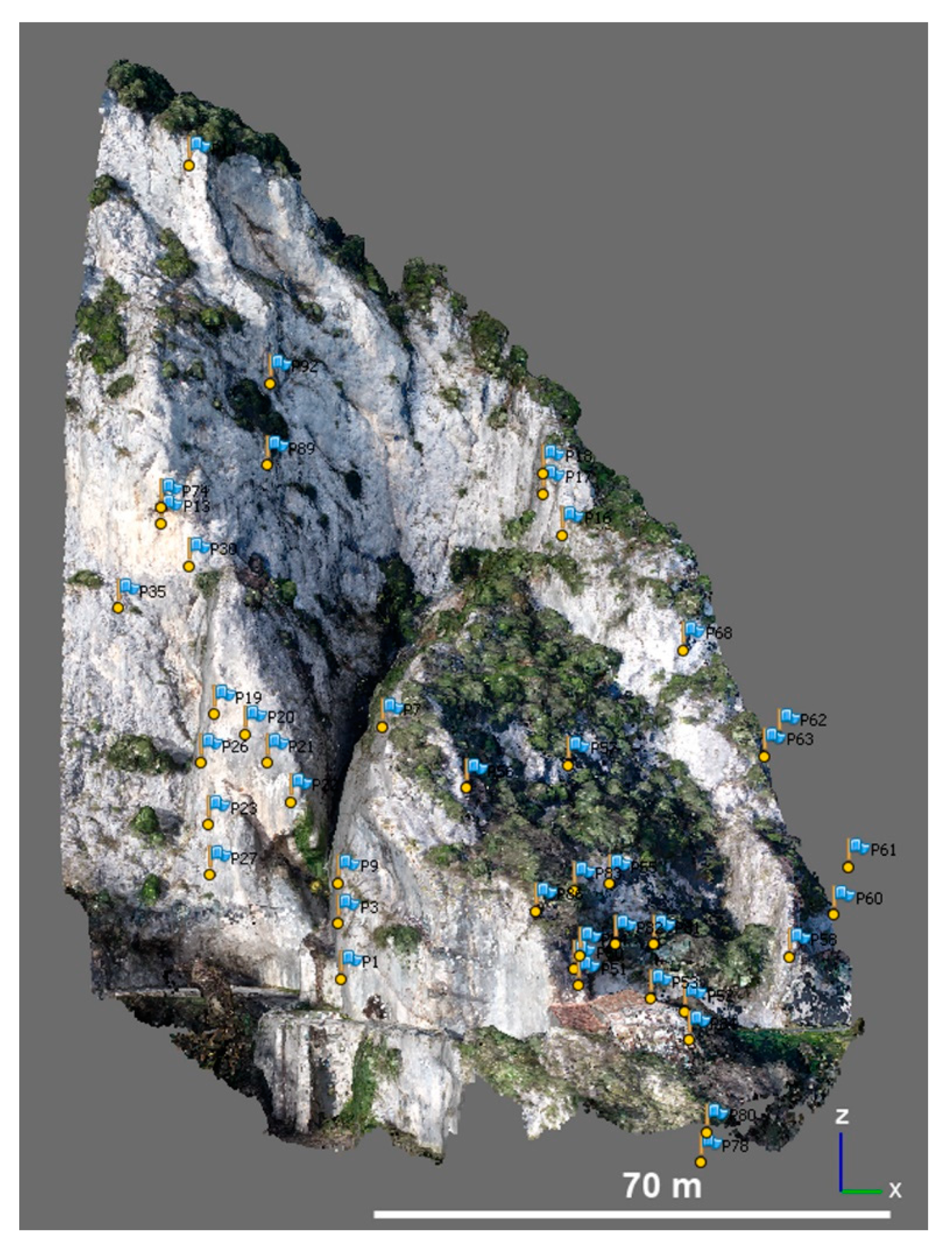
The complex morphology of the area, with a deep and narrow gorge, did not allow for an automatic flight with waypoints: it was flown manually with an automatic triggering of photos every 2 s. Moreover, the use of a UAV equipped with a Real Time Kinematic (RTK) GNSS, which could have allowed acquisition of accurate coordinates of the camera location at every shot, was also not possible: the limited satellite visibility and the high Positional Dilution Of Precision (PDOP) within the gorge could have determined very low spatial accuracy in data. Therefore, the exterior orientation of all images (i.e., 1232 photos) was done by using 80 Ground Control Points (GCPs), which distribution is shown in
Figure 2, measured again by the combining TS measurements, GNSS surveys in static modality, and differential data post-processing with a final millimeter-level positioning accuracy.
Eight artificial targets were pre-placed in the accessible zones of the study area, while the rest were obtained using natural features visible in the photos throughout the slope and by the TS during fieldwork. Their location was decided considering a balance between an optimum spatial distribution, both in space and elevation from the road, and easy identification of points on the images. The software Agisoft™ MetaShape (version 1.5.3;
http://www.agisoft.com, last access: 24 June 2019) was used to process the images obtained from the UAV surveys. This software can solve the camera interior and exterior orientation parameters and generate georeferenced spatial data such as 3D point clouds, DEMs, DTMs and orthophotos. Agisoft™ MetaShape based on (i) SfM technology for the exterior orientation of images and the creation of the sparse 3D point cloud and (ii) MVS photogrammetry for the dense cloud reconstruction [
67,
68].
The first processing step consisted of image alignment, through which the interior and relative orientation parameters were solved. In order to improve the whole alignment process and to obtain low re-projection error, millions of tie points were automatically extracted without setting a point limit. Following image alignment, the second processing step involved georeferencing of the 3D model in such a way as to solve the exterior orientation parameters by using the GCPs coordinates measured during the GNSS-TS topographic surveys. The exterior orientation of images was necessary to measure the orientation, with respect to the North, and inclination of slopes and discontinuities which are needed for the stability analysis.
Subsequently, the “optimize” tool of Agisoft™ MetaShape was utilized to adjust the estimated camera positions and to remove possible non-linear deformations, minimizing the errors due to re-projection and misalignment of the photos. Moreover, the optimization improved the model by deleting all the tie points with a re-projection error greater than one pixel.
In a subsequent step, the dense 3D point cloud was generated with medium quality and aggressive depth filtering settings. Automatic classification of cloud was done trying to remove vegetation, as much as possible, from the area of interest.
Finally, the different point clouds obtained by TLS and UAV image processing, both georeferenced in the Italian National Gauss-Boaga reference system, were unified using the open source CloudCompare™ software to produce a final complete 3D model of the rock mass including RGB data for texturing. The different point clouds were imported and no further alignment was executed. This is due to the fact the engineering-geological analyses were carried out on blocks and discontinuities only visible on the UAV-point cloud. The TLS-point cloud, instead, was fundamental for the complete characterization of the slope geometry, which is essential for the 3D rockfall runout analysis. As already mentioned, this was mainly due to the presence of trees on the lower part of the slope, which covered a portion of the rock mass in proximity to the local road. This caused distortions and holes on the UAV-point cloud, with possible consequences on the block trajectories. Therefore, the UAV-point cloud was replaced by the TLS-point cloud where needed (lower lateral parts of the slope). In this view, slight offsets between the two point clouds were considered negligible because, as explained later in
Section 4.3.2, the spatial resolution of the input raster maps for the runout analysis was set equal to 50 cm/pixel, more than the possible error of mis-alignment of the two different point clouds.
3.2. Engineering-Geological Characterization of the Rock Mass and Stability Analysis
A direct engineering-geological survey was possible only on the lower parts of the slope. Unfortunately, the accessible areas allowed for the analysis of only few discontinuities, considered not fully representative of the conditions of the higher parts. For this reason, visual inspection in the field provided only a qualitative assessment of the rock mass conditions and the measurement of few joint characteristics (e.g., joint aperture, infill, weathering, compressive strength). Given the impossibility to collect all the necessary discontinuity properties, a proper characterization of the rock mass using traditional methods such as, for example, the Rock Mass Rating (RMR, [
69,
70]) was not possible. In the place of it, the Hoek and Brown Geological Strength Index (GSI, [
71]) was determined since it bases on qualitative geological observations.
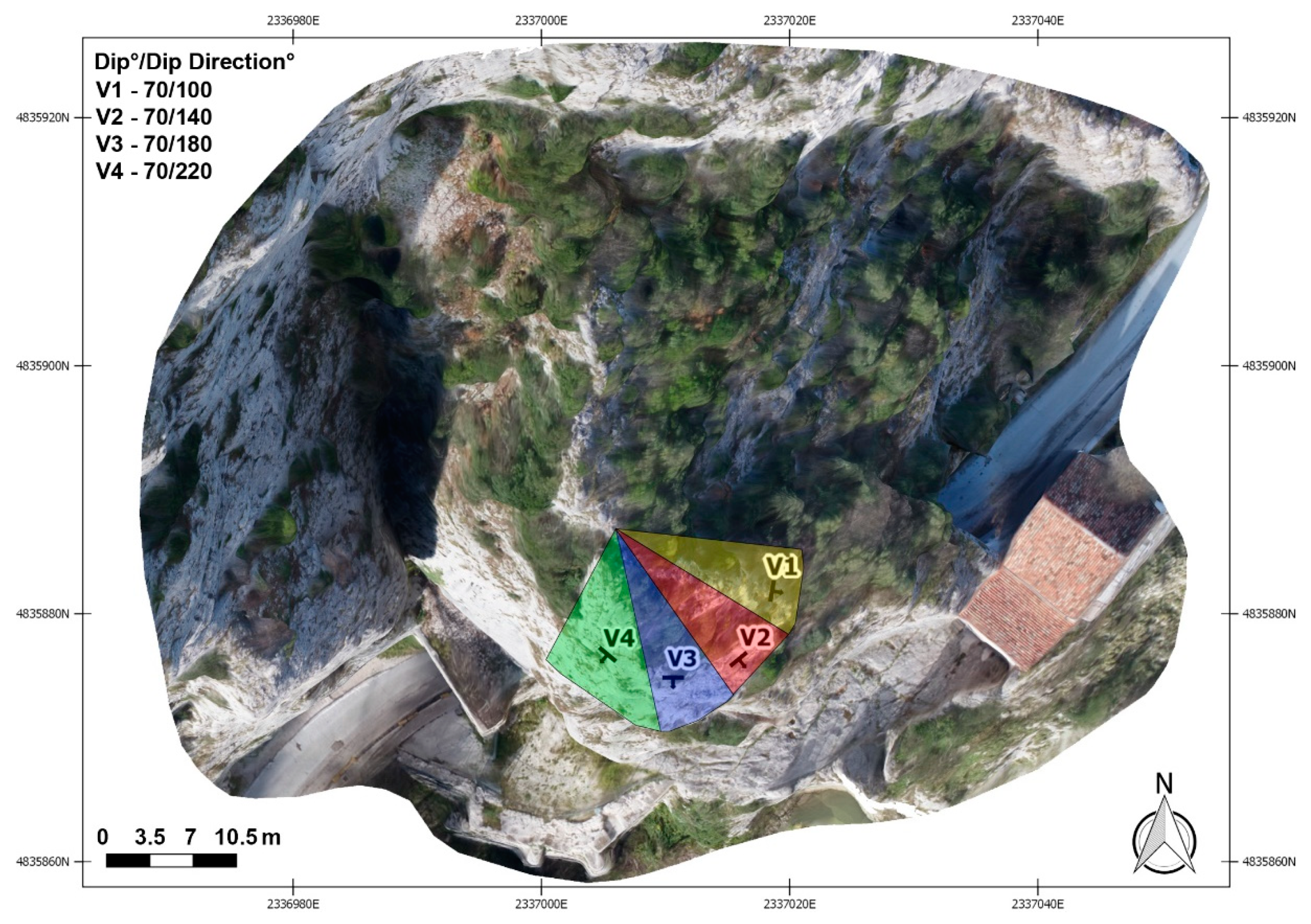
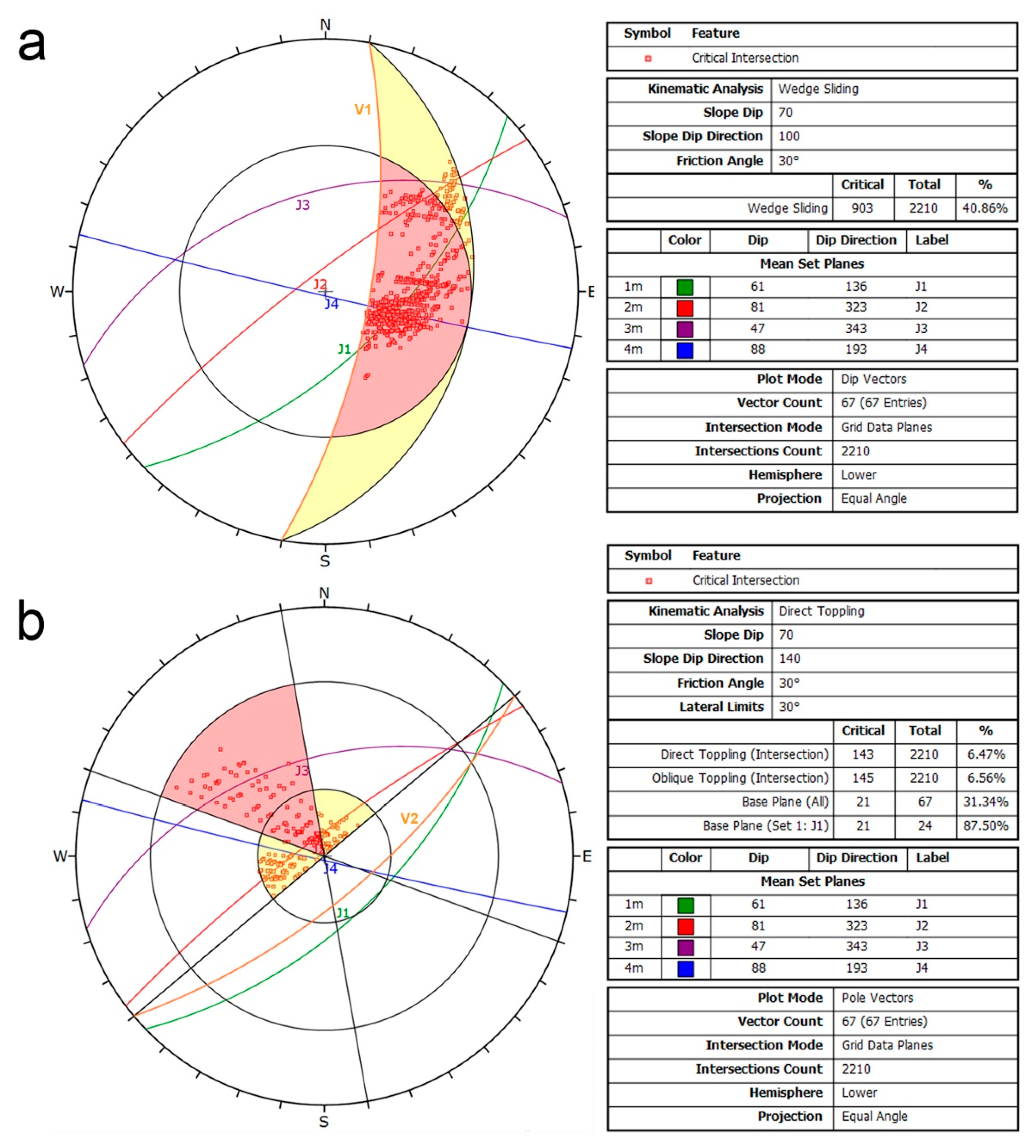
The structural analysis of the higher parts of the slope was carried out by using the Compass plugin [
72] of the freeware CloudCompare™ software. Compass is a plugin which allows measurement of discontinuity orientations directly on the point cloud. In this way, the orientation of about 70 discontinuities in strategic areas of the slope was acquired to create a stereonet used to identify the different discontinuity sets. Following this, a kinematic stability analysis, based on the Markland test [
73] was performed. Since the results of the kinematic analysis are influenced by geotechnical properties and topographic factors (i.e., dip and dip direction of rock outcrops), the slope was divided in four sectors (
Figure 3) with different orientations.
Such analysis allowed identification of the main types of failure (i.e., toppling, planar sliding, wedge sliding).
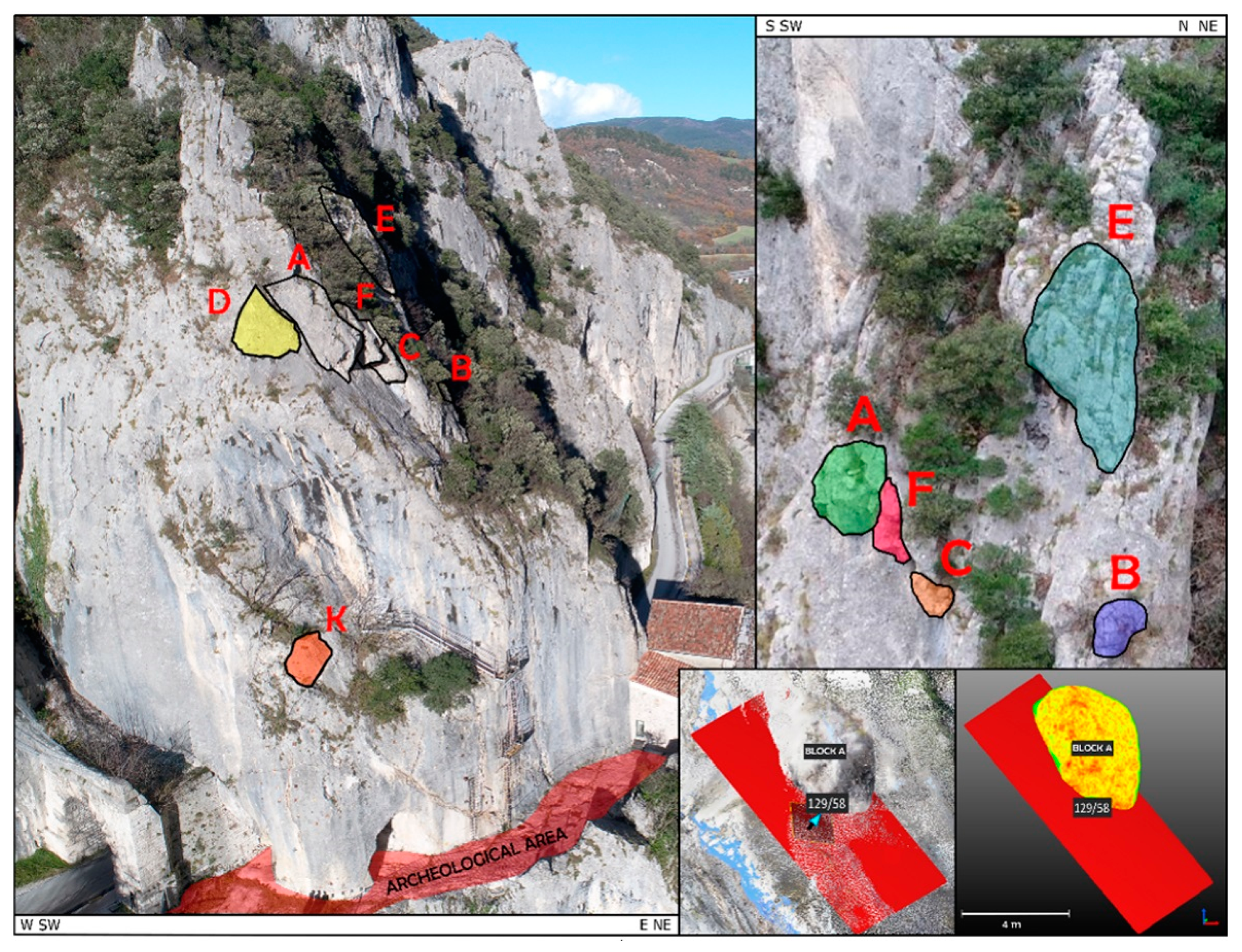
In addition, CloudCompare was used to estimate volumes, geometries, and positions of all potentially unstable blocks that could trigger rockfall events in the future. This provided a basis to identify source blocks to be used in the subsequent dynamic stability analysis and rockfall runout simulation. The geometric information can be extracted from the point cloud manually, or utilizing software to automate the process [
74,
75]. For example, in [
76] the authors used Polyworks (InnovMetric Software, 2017) to define the sets of the discontinuities based on 3D point clouds and then used the spacing of each set to roughly calculate the average size of blocks. In their work, the discontinuity information was extracted manually from the point clouds and the block size was calculated approximately. Differently, in [
77] a fully automatic method for extracting rock block information from 3D point clouds was presented.
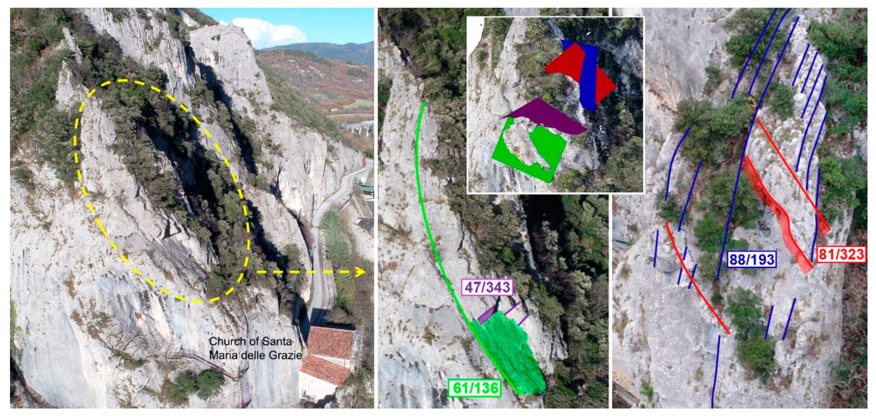
In this paper blocks were identified on the final point cloud by a careful photointerpretation that was also revised and validated by experts. The following procedure was used: (i) the point cloud was segmented in several areas containing a potentially unstable block each; (ii) every joint located below a potentially sliding block was sampled and co-planar points selected; (iii) the cloud representing each block was cut and the normals to the points, oriented toward the exterior, computed; (iv) the clouds representing both the block and the underlying joint were merged and used to build a mesh through the Poisson Surface Reconstruction Plugin [
78]; (v) finally, by means of the editing tools of CloudCompare, the volume of every mesh was measured.
The dynamic stability analysis of rock blocks was carried out by Rocscience™ codes (i.e., Rocplane, Swedge, Roctopple for planar sliding, edge sliding and block toppling, respectively). SFs were calculated both in static and dynamic conditions considering the presence of water, and the local seismic acceleration. Using GeoStru™ PS software (GeoStru, 2019) the maximum horizontal acceleration “ag” of the site was derived (i.e., 0.25 g in this study). The procedure was carried out following the new Italian “Norme Tecniche per le Costruzioni” [
79].
3.3. Rockfall Runout Analysis
The mathematical model that can be adopted to analyze the rockfall runout must be able to describe the behavior of a falling block in terms of trajectory direction and length, bounce height, speed, energy, and type of movement. Two principal methods can be used to solve this problem: (i) lumped mass methods and (ii) rigorous methods [
80]. The lumped mass approach considers the single block as a point with specific mass and velocity. Therefore, it is a simplified model where the velocity of the block is reduced after every impact with the surface by using two coefficients Kn (normal coefficient of restitution) and Kt (tangential coefficient of restitution). Differently, a more rigorous approach considers the shape and dimension of the falling block, which must be known a priori. It is a complete method that considers the moment changes, depending on shape of block and surface, angle of trajectory, roughness of the surface, and friction between block and surface [
80].
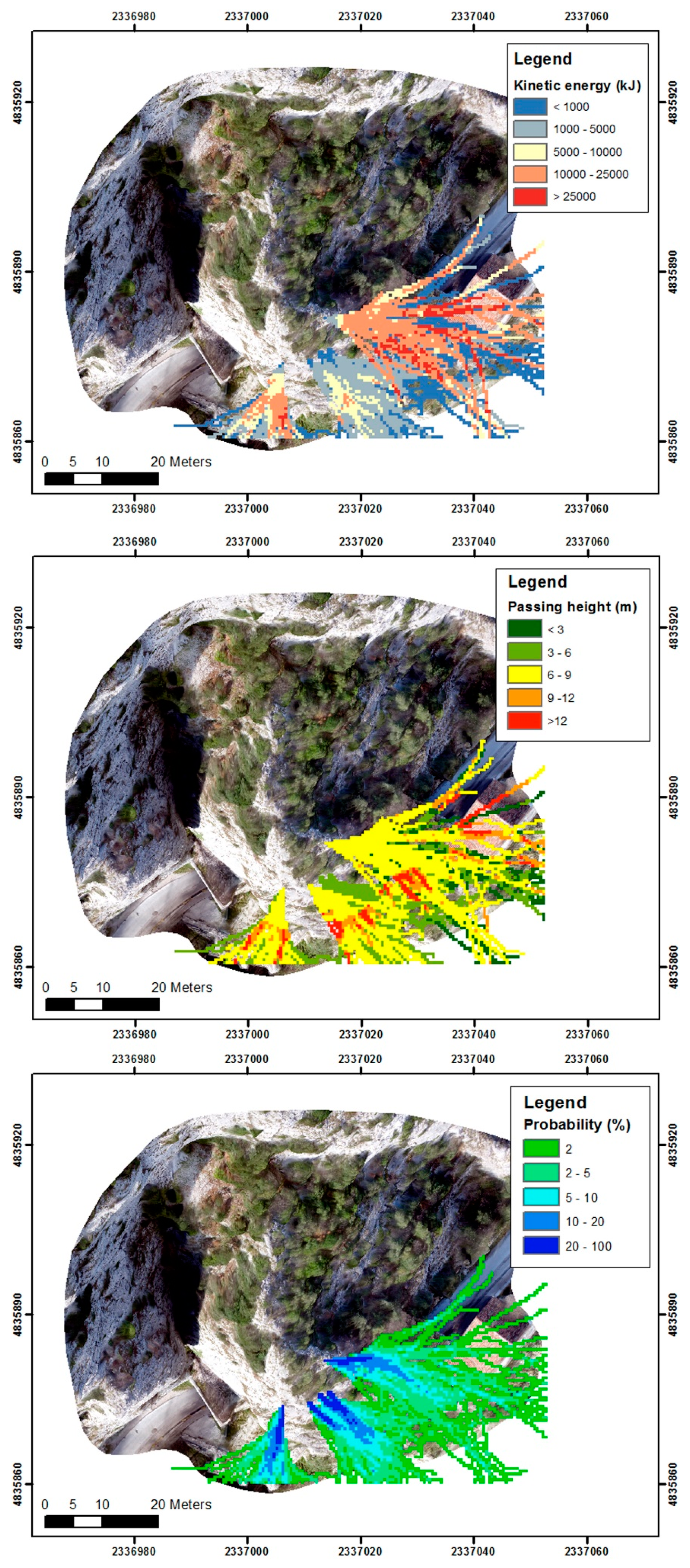
The method used in this paper follows a 3D rigorous approach. The simulation software is called Rockyfor3D [
81] and combines physically based deterministic algorithms with stochastic approaches. In this sense, Rockyfor3D is also defined as “probabilistic process-based rockfall trajectory model.” The trajectory is simulated as a 3D vector data by sequences of parabolic free fall through the air and rebounds on the surface. Sliding of the rock is not considered, as well as block fragmentation, and rolling of the mass is represented by a sequence of short-distance rebounds [
81]. Moreover, the model considers impacts against trees. The simulations can be run by using 14 ASCII rasters characterized by the same cell size and extent, which describes the characteristics of slope surface and falling blocks. The input raster maps, created in a GIS environment using the data from the geomatic and geological surveys, are described in
Table 1.
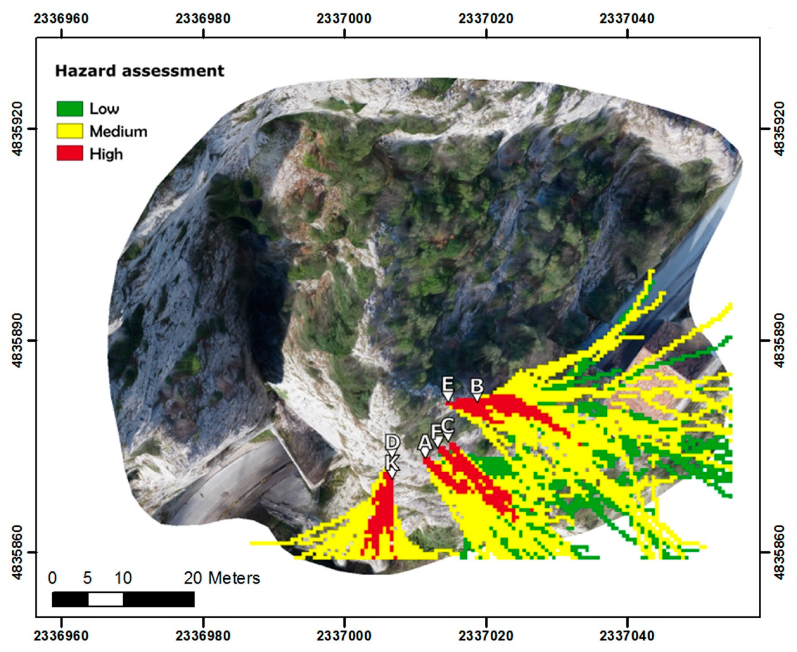
The runout simulations with the current slope configuration were performed using the input blocks identified on the UAV images and measured on the 3D point cloud. However, it has to be mentioned that, before proceeding with the rockfall runout simulation, a model calibration step was done; this process, also defined as “back analysis” in respect of a past rockfall event, which is essential to calibrate the entire 3D model together with the simulation input parameters and raster. In this case, given the steep geometry of the slope, which is characterized essentially by steep bedrock with limited vegetation overhanging water dump, it is difficult to simulate a past rockfall event, since the arrival point is generally missing (i.e., below water level). In terms of rockfall runout analysis, well-represented geometrical info were obtained: not only slopes, but also the potentially unstable blocks were well known in terms of shape and size. Physical parameters were calibrated (i.e., coefficients of normal and tangential restitution) in such a way that input data can be considered adequate for a reliable rockfall runout study.

 ,
, 


