A Hybrid Multi-Product Framework for Spatiotemporal Built-Up Expansion Mapping Across Contrasting Physiographic Landscapes of Nepal Using Sentinel-2 and Google Earth Engine

Abstract

Built-up expansion is reshaping landscapes across Nepal; however, consistent multi-temporal mapping remains challenging due to rugged terrain, fragmented settlements, and heterogeneous land-cover conditions. This study develops and evaluates a multi-product and terrain-informed workflow in Google Earth Engine for mapping built-up expansion across three physiographically contrasting districts of Nepal: Arghakhanchi, Lalitpur, and Chitwan, from 2017 to 2025. Annual predictor stacks were generated by integrating Sentinel-2 spectral bands and derived indices, Dynamic World built-up probabilities, and SRTM-derived elevation and slope variables. ESRI Global Land Cover datasets were used separately for auxiliary cross-product comparison and assessment of the mapped outputs. Preliminary yearly built-up masks were generated using district- and year-specific Random Forest classifications, followed by the post-classification constraints, and were subsequently integrated through cumulative expansion mapping. Accuracy assessment for 2017, 2021, and 2025 yielded overall accuracy values of 86.4–92.4%, built-up F1-scores of 84.7–91.3%, and Kappa coefficients of 0.81–0.91. Between 2017 and 2025, cumulative built-up extent expanded by 8054.65 ha in Chitwan, 2406.20 ha in Arghakhanchi, and 2215.96 ha in Lalitpur; Arghakhanchi recorded the highest proportional increase (117.6%). The mapped expansion was comparatively dispersed in Arghakhanchi, concentrated within metropolitan and peri-urban areas in Lalitpur, and broader and corridor-oriented in Chitwan. Because previously detected built-up pixels were retained in subsequent cumulative outputs, the resulting extents were non-decreasing by construction and did not represent demolition or other land use reversals. Consequently, annual built-up expansion should not be interpreted as net annual land-cover change. The proposed framework provides a practical and transferable approach for comparative built-up expansion monitoring and urban growth assessment across contrasting physiographic settings.

1. Introduction

Urban growth is rapidly changing land use patterns worldwide, particularly in developing countries, where cities are expanding into agricultural and natural landscapes. This process has accelerated the conversion of forests, wetlands, and agricultural land into built-up areas, generating significant environmental and socio-economic challenges. Recent studies indicate that future urban land expansion is expected to intensify significantly, especially across the developing countries, with profound implications for biodiversity, ecosystem services, climate resilience, and sustainable urban governance [1,2,3]. The expansion of urban areas is closely associated with several environmental and planning challenges, including agricultural land loss, ecosystem fragmentation, increased surface runoff, urban heat island effects, and growing pressure on infrastructure and public services [4,5]. Consequently, accurate and consistent monitoring of urban expansion has become essential for informing land use planning, disaster risk reduction, and sustainable urban governance.

Advances in remote sensing and geospatial technologies have substantially improved the capacity to monitor urban growth across large spatial and temporal scales. Satellite-based urban mapping has progressed from visual interpretation and simple threshold-based approaches toward more advanced machine learning and cloud-computing approaches [6]. Sentinel-2 imagery has become particularly useful for urban land-cover analysis because of its 10 m spatial resolution, multispectral capability, and frequent revisit cycle [7,8]. However, medium-resolution imagery still presents limitations in fragmented landscapes, narrow built-up features, small water bodies, and heterogeneous terrain because of mixed-pixel effects and spectral ambiguity [9,10]. At the same time, cloud-based platforms such as Google Earth Engine (GEE) have made it possible to process large volumes of satellite imagery efficiently without requiring extensive local computing resources [11]. Machine learning algorithms, particularly Random Forest (RF), have also shown strong performance in land-use and land-cover classification because of their robustness, non-parametric structure, and ability to handle multidimensional datasets with complex spectral relationships [12,13,14].

Despite these advances, urban expansion mapping remains methodologically challenging in mountainous and physiographically heterogeneous environments. Complex topography, fragmented settlement patterns, terrain-induced spectral variability, seasonal differences, and mixed land-cover conditions often reduce classification reliability [15,16,17,18]. In Nepal, urban growth frequently occurs in dispersed rural settlements, roadside linear expansion, peri-urban transition zones, and fragmented agricultural mosaics [19,20,21,22]. These settlement patterns complicate the separation of built-up areas from bare soil, exposed riverbeds, rocky terrain, fallow agricultural land, construction sites, and transportation corridors using conventional classification approaches [14,23]. Furthermore, independent annual land-cover maps may exhibit temporal fluctuations because of atmospheric variation, seasonal spectral differences, mixed pixels, and classification instability [24,25,26]. For analyses focused on the progressively detected built-up footprint, such fluctuations can be managed through cumulative mapping, provided that the resulting product is interpreted as an accumulated expansion footprint rather than as net annual land-cover change.

Several studies in Nepal have examined urban expansion and land-use change using remote sensing and GIS techniques. Previous research has documented urban growth dynamics in Kathmandu Valley, Pokhara, Bharatpur, and other rapidly urbanizing municipalities through the application of supervised classification, spectral indices, landscape metrics, and cloud-based geospatial analysis [19,27,28,29,30]. These studies have provided valuable insights into local and regional urbanization processes. However, many studies remain geographically localized or rely on a limited set of predictor variables. Comparatively few studies have combined Sentinel-2 spectral information, complementary land-cover products, terrain variables, and cumulative built-up-footprint mapping across contrasting physiographic settings in Nepal [31]. Although GEE, machine learning, and advanced remote sensing techniques are increasingly used in urban studies, their combined use with probabilistic land-cover products and cumulative built-up-footprint mapping for comparative urban expansion analysis across Nepal’s diverse physiographic regions remains limited [27,32]. Furthermore, evaluating this multi-product, terrain-informed, cumulative workflow across Nepal’s mid-hill, metropolitan peri-urban, and Inner Terai regions represents a novel methodological approach.

Recent probabilistic and time-series land-cover datasets provide new opportunities to improve urban mapping in complex environments. Dynamic World provides near-real-time land-cover probability information derived from Sentinel-2 imagery, while ESRI Global Land Cover products offer globally consistent 10 m land-cover time-series information that can support built-up area identification and temporal comparison [33,34]. In the present workflow, Dynamic World built-up probabilities were incorporated as classification predictors, whereas ESRI Global Land Cover was used separately for auxiliary cross-product comparison and visual calibration of the mapped outputs. However, their application for long-term and physiographically comparative urban expansion mapping in Nepal remains insufficiently explored. To address these gaps, this study develops and evaluates a hybrid multi-product framework for spatiotemporal urban expansion mapping within the Google Earth Engine environment.

This study advances existing approaches to urban expansion mapping through the development of a hybrid multi-product framework that integrates multispectral imagery, probabilistic land-cover products, terrain variables, and Random Forest classification with a temporal accumulation procedure. Unlike conventional approaches that rely on independently classified annual datasets, the proposed framework explicitly incorporates cumulative mapping to represent progressively detected built-up extent through time. The integration of Dynamic World built-up probability layers within a terrain-informed classification framework provides complementary spectral, probabilistic, and terrain information for built-up classification, particularly in heterogeneous environments. ESRI Global Land Cover was used separately for auxiliary cross-product comparison and iterative visual calibration. By combining complementary geospatial datasets with temporal accumulation, the framework offers a structured approach for long-term urban expansion monitoring in physiographically heterogeneous regions. The main contributions of this study include:

• Development of an integrated multi-product and terrain-informed workflow that combines Sentinel-2 spectral bands and derived indices, Dynamic World built-up probabilities, SRTM-derived terrain variables, district-specific Random Forest classification, and post-classification constraints to generate preliminary yearly built-up detections across complex geographic settings.
• Development of a context-sensitive terrain-informed component that incorporates elevation, slope, and district-specific filtering thresholds to reduce terrain-related spectral confusion, address fragmented settlements, and minimize false built-up detections in physiographically heterogeneous landscapes.
• Introduction of a progressive accumulation approach in which preliminary yearly built-up detections are combined to derive cumulative built-up extent and annual built-up expansion, supporting the analysis of long-term expansion patterns while distinguishing them from net annual land-cover change.
• Comparative assessment of built-up expansion across contrasting physiographic settings in Nepal, including the mid-hill environment of Arghakhanchi, the metropolitan peri-urban setting of Lalitpur, and the Inner Terai landscape of Chitwan, thereby providing planning-relevant evidence on differences in both expansion magnitude and spatial characteristics.

The remainder of this paper is organized as follows. Section 2 describes materials and methods which include the study area, data sources, and the proposed methodological framework for spatiotemporal built-up expansion mapping. Section 3 presents the classification results and analyzes the spatial and temporal patterns of urban growth across the study districts. Section 4 provides a detailed discussion of the findings and methodological implications and outlines the limitations and directions for future research. Finally, Section 5 summarizes the main findings and highlights the key contributions of the study.

2. Materials and Methods

2.1. Study Area

Nepal is a landlocked Himalayan country located in South Asia, bordered by China to the north and India to the south, east, and west. Geographically, the country lies between 26°22′ and 30°27′ north latitude and 80°04′ and 88°12′ east longitude, covering a total area of approximately 147,516 km² [35]. Administratively, Nepal is divided into seven provinces, 77 districts, and 753 local government units under the federal governance system established by the Constitution of Nepal in 2015 [36,37]. The country exhibits remarkable physiographic diversity and is commonly divided into three major geographical regions: the Mountain region in the north, the Hill region in the center, and the Tarai plains in the south [38,39]. These regions vary significantly in terms of topography, climate, settlement patterns, land use, and socio-economic characteristics, making Nepal one of the most geographically diverse countries in the world [28].

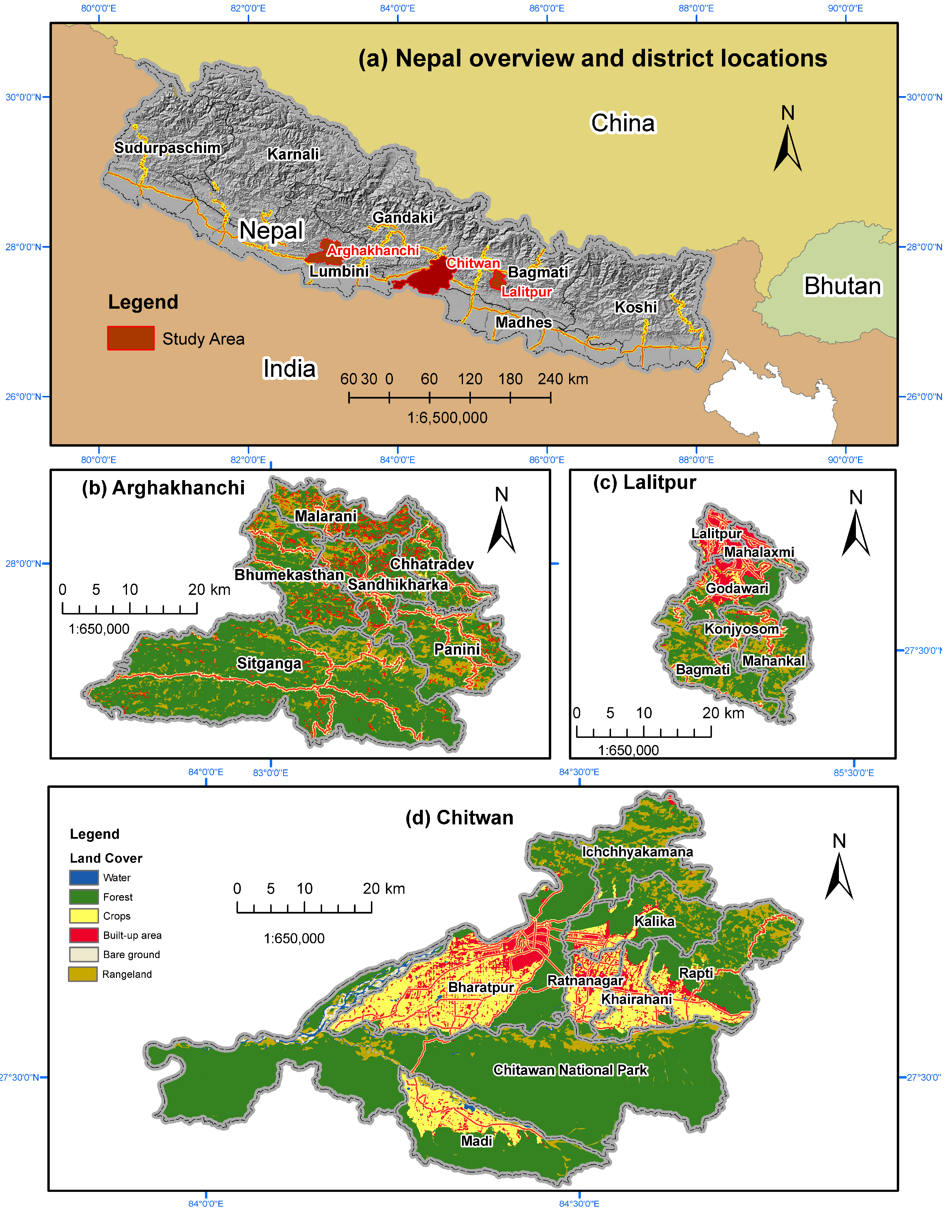
The study was conducted in three physiographically contrasting districts of Nepal: Arghakhanchi (mid-hill), Lalitpur (metropolitan peri-urban), and Chitwan (Inner Tarai) as illustrated in Figure 1. These districts were purposively selected to represent distinct urbanization dynamics and settlement patterns across diverse topographic and socio-economic settings. The inclusion of mid-hill, metropolitan peri-urban, and Inner Terai landscapes provides a basis for applying the proposed workflow and comparing built-up expansion patterns across contrasting physiographic and settlement contexts.

Arghakhanchi District lies within the mid-hill region of western Nepal which is characterized by rugged terrain, fragmented settlement structures, dispersed rural habitation, and relatively small urban centers [40]. Urban expansion, as commonly observed in Nepal’s hill districts, is associated with market centers, roadside settlements, and emerging municipal growth corridors [28]. Hill districts such as Arghakhanchi present significant challenges for urban mapping due to steep terrain, heterogeneous land-cover patterns, and scattered settlement morphology [20,28].

Lalitpur District represents one of the most rapidly urbanizing metropolitan regions of Nepal and forms part of the Kathmandu Valley urban agglomeration [27,41]. The district exhibits complex peri-urban expansion patterns characterized by urban sprawl, infrastructure-driven growth, conversion of agricultural land, and expansion of transportation corridors [29,42]. The northern part of Lalitpur contains dense metropolitan built-up areas, while the southern region transitions into rural hill landscapes with fragmented settlements and forested terrain [43]. This physiographic diversity makes Lalitpur particularly suitable for evaluating urban classification performance under mixed urban–rural conditions.

Chitwan District, located in the inner Terai region of south-central Nepal, represents a rapidly urbanizing alluvial plain characterized by corridor-based urban expansion, agricultural land transformation, and concentrated municipal growth around Bharatpur Metropolitan City and associated highway corridors [28,44]. Compared to hill districts, Chitwan exhibits relatively flatter terrain and larger contiguous built-up areas [45]; however, urban classification remains challenging due to spectral confusion associated with exposed riverbeds, floodplains, agricultural fallow land, and rapidly changing peri-urban landscapes [20].

Together, the three districts represent diverse urbanization regimes in Nepal, including dispersed settlement expansion in the mid-hills, metropolitan peri-urban sprawl, and the corridor-oriented urbanization across the agricultural plains of the Inner Terai. This diversity provides an appropriate basis for assessing built-up expansion patterns and workflow performance across contrasting physiographic and settlement contexts.

2.2. Data Sources

The study utilized multiple remote sensing, probabilistic land-cover, terrain, and reference datasets within the Google Earth Engine (GEE) cloud-computing environment to develop an integrated framework for spatiotemporal urban expansion analysis as listed in

Table 1. Data products, supporting materials, and their analytical roles in the built-up expansion mapping workflow.

Data Source/Resource	Data Type	Spatial Resolution or Form	Analytical Role
Sentinel-2 Surface Reflectance	Level-2A multispectral satellite imagery	10 m (B2, B3, B4, and B8) 20 m (B11 and B12)	Primary spectral predictor; source of annual median composites and derived indices (NDVI, NDBI, MNDWI, and BSI).
Dynamic World V1	Sentinel-2-derived probabilistic land-cover product	10 m	Probabilistic classification predictor; annual mean of the “built” probability band used as an auxiliary predictor.
ESRI Global Land Cover Time Series	Sentinel-2-derived categorical land-cover product	10 m; annual products available for 2017–2024 at the time of access	Auxiliary cross-product comparison of mapped built-up outputs; not used as a classifier predictor or independent validation dataset.
SRTM DEM	Digital Elevation Model (DEM)	Approximately 30 m native resolution	Source of elevation and slope predictors; slope was also used as a district-specific post-classification constraint.
Digitized Training Samples	Manually interpreted vector features representing built-up and non-built classes	Vector features	Training datasets for district-specific Random Forest classifiers.
Stratified Validation Points	Point sampling dataset	Point features	Candidate locations for accuracy assessment; reference labels were assigned through visual interpretation of suitable imagery.
Google Earth Pro Imagery	High-resolution and historical reference imagery	Variable according to location and acquisition year	Visual interpretation of training samples and validation-point reference labels; not used as a classification predictor.

Note: Dynamic World and ESRI Global Land Cover products are both derived from Sentinel-2 imagery and should be considered as complementary products rather than independent data sources. Sentinel-2 and SRTM data were used at their native resolutions within the GEE processing chain; no explicit reproject() or resample() operation was applied, and the final classified outputs were exported at a nominal spatial resolution of 10 m.

. Sentinel-2 Surface Reflectance (SR) imagery constituted the primary dataset for annual urban classification because of its high spatial resolution (10 m), multispectral capability, and frequent revisit cycle [7,8]. Sentinel-2 imagery was accessed through the COPERNICUS/S2_SR_HARMONIZED collection in GEE. The collection was first accessed on 30 January 2026, and processing, calibration, and refinement continued over several months; the latest verified output used in the analysis was exported on 12 May 2026. The collection provides atmospherically corrected Level-2A products generated using the Sen2Cor atmospheric-correction algorithm [46].

For each study year, the image collection was filtered by Area of Interest (AOI), acquisition period (October–December), and cloud-cover threshold (CLOUDY_PIXEL_PERCENTAGE < 30). Post-monsoon imagery acquired between October and December was selected to minimize monsoon cloud contamination and reduce seasonal spectral inconsistency. Median composites were subsequently generated from the filtered image collection to minimize residual atmospheric noise and produce representative annual imagery for classification. The GEE cloud-based processing environment enabled efficient management and analysis of large multi-temporal datasets across physiographically heterogeneous study areas [4,11].

To improve urban feature extraction, several complementary datasets were integrated with Sentinel-2 imagery. Dynamic World V1, a near real-time global 10 m land use/land cover dataset derived from Sentinel-2 imagery, was accessed through the Google Earth Engine Data Catalog (https://developers.google.com/earth-engine/datasets/catalog/GOOGLE_DYNAMICWORLD_V1; first accessed on 30 January 2026). The dataset provides per-pixel class probabilities and land-cover labels for nine classes and has been widely used for land-cover mapping applications [33]. The “built” probability band derived from Dynamic World was incorporated into the classification framework to strengthen urban detection in fragmented and rapidly changing settlement areas. Similarly, the ESRI Global Land Cover 10 m time-series dataset, accessed through the ArcGIS Living Atlas of the World (https://livingatlas.arcgis.com/landcoverexplorer/; first accessed on 12 December 2025), was used separately as an auxiliary cross-product comparison and iterative visual-calibration source [34]. At that time of access, annual maps were available for 2017–2024. This product was not used as a classifier predictor variable in the classification process nor as an independent validation dataset.

Several spectral indices relevant to urban analysis were derived directly from Sentinel-2 multispectral imagery to enhance spectral discrimination among different land-cover classes. The Normalized Difference Vegetation Index NDVI was derived to distinguish vegetated surfaces [47,48], the NDBI to enhance built-up areas [48,49], the MNDWI to identify water bodies [50,51], and the BSI to characterize exposed soil and barren surfaces [9,52]. In addition, terrain variables were derived from the Shuttle Radar Topography Mission (SRTM) Digital Elevation Model (USGS/SRTMGL1_003) available through Google Earth Engine (https://developers.google.com/earth-engine/datasets/catalog/USGS_SRTMGL1_003, first accessed on 31 January 2026). Elevation and slope layers generated from the SRTM DEM were integrated into the classification framework to reduce terrain-induced misclassification associated with steep slopes, topographic shadows, and mountainous terrain conditions [16,53,54].

Training and validation datasets were generated through manual digitization and stratified sampling procedures within the Google Earth Engine (GEE) environment. Built-up samples were digitized separately, while vegetation, water, and bare-land samples were merged into a generalized non-built category for Random Forest training. The digitized vector samples were extracted against the integrated image stack comprising Sentinel-2 spectral bands, derived spectral indices, Dynamic World built-up probabilities, and terrain variables. Similarly configured Random Forest classifiers were developed for each study year using the corresponding annual predictor stack, thereby maintaining a consistent classification framework from 2017 to 2025. Random Forest has been widely recognized as an effective machine-learning algorithm for land-use and urban classification because of its robustness against overfitting, ability to handle high-dimensional predictor variables, and strong classification performance in heterogeneous landscapes [12,13]. The classifier operated in probability mode, after which built-up areas were extracted using probability thresholds together with NDVI, MNDWI, and slope constraints to reduce false positives associated with water bodies, vegetation, steep terrain, and exposed surfaces. A connected-pixel filtering approach was further applied to remove isolated speckle pixels and improve spatial coherence of the classified built-up areas, a common post-classification refinement procedure in remote sensing-based urban mapping [8].

Preliminary built-up masks were generated separately for each study year from the corresponding predictor stacks. These yearly detections were subsequently combined to derive cumulative built-up extents and annual built-up expansion, as described in Section 2.8. Accuracy assessment was conducted for 2017, 2021, and 2025 using 300 stratified validation locations per district, comprising 150 built-up and 150 non-built locations. Reference labels were interpreted from high-resolution and historical imagery, and confusion-matrix analysis was used to calculate the classification accuracy metrics. Stratified random sampling combined with confusion matrix analysis are widely adopted approaches for evaluating thematic classification accuracy in remote sensing studies because they provide statistically representative assessment of classification performance across multiple land-cover classes [55,56].

In addition to the primary remote sensing and terrain datasets, several supplementary geospatial and analytical resources were utilized to support validation, visualization, and result interpretation. Historical high-resolution imagery available through Google Earth Pro V7.3 was used for visual interpretation, training sample verification, reference interpretation of validation points and visual examination of built-up expansion patterns across different years. ArcGIS Desktop V10.8 was employed for cartographic visualization, spatial layout preparation, map composition, and post-classification spatial analysis. Exported classification outputs and annual urban expansion statistics generated in Google Earth Engine were further processed in Microsoft Excel for tabular compilation, graphical visualization, trend analysis, and statistical comparison. Together, these supplementary resources supported the integration of cloud-based remote sensing analysis with conventional GIS-based mapping and statistical interpretation workflows.

2.3. Methodological Framework

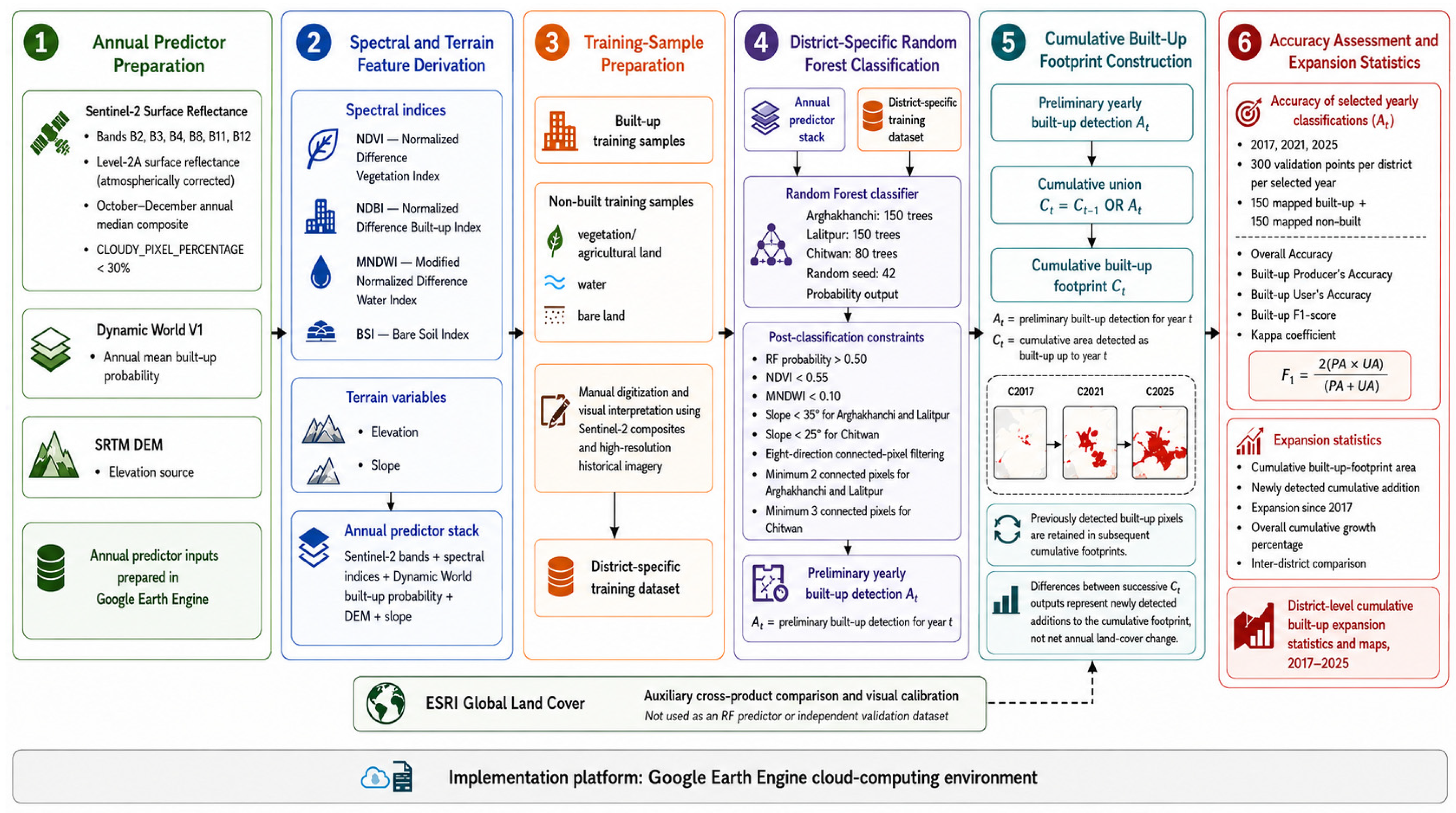
The study adopted a hybrid multi-product framework for multi-temporal built-up area extraction and built-up expansion mapping integrating multispectral satellite imagery, probabilistic land-cover data, spectral indices, terrain conditioning variables, machine learning classification techniques, and cumulative built-up expansion mapping within the Google Earth Engine (GEE) cloud computing environment as illustrated in Figure 2. The methodological workflow consisted of six major stages: (i) data acquisition and preprocessing, (ii) derivation of spectral and terrain variables, (iii) preparation of training samples, (iv) Random Forest classification, (v) cumulative built-up expansion mapping analysis, and (vi) accuracy assessment.

The method was developed to improve built-up area detection in regions where terrain complexity and fragmented settlement patterns reduce classification accuracy. The proposed framework integrates multiple complementary products and classification variables within a common classification and cumulative expansion workflow. Cloud-based geospatial platforms such as Google Earth Engine have substantially transformed large-scale remote sensing analysis by enabling rapid access, processing, and visualization of multi-temporal geospatial big data within scalable computational environments [6,11]. Recent studies have increasingly utilized GEE-integrated machine learning frameworks for urban monitoring, land-cover classification, and environmental change analysis due to their computational efficiency and accessibility [6,27,32].

2.4. Data Preprocessing

Sentinel-2 Surface Reflectance (Level-2A) imagery was used as the primary dataset for annual built-up area classification. The primary dataset was obtained from the European Space Agency (ESA) Copernicus program and accessed through the Google Earth Engine (GEE) platform using the Sentinel-2 Surface Reflectance image collection [46]. Annual image composites were generated for the post-monsoon period (October–December) to minimize cloud contamination and reduce spectral variability associated with monsoon moisture and seasonal agricultural changes. Images with cloud cover exceeding 30% were excluded, and annual median compositing was applied to reduce atmospheric noise and cloud related errors. No additional pixel-level cloud, shadow, scene-classification masking (such as SCL or QA60) was applied; residual cloud and atmospheric effects were instead limited through scene-level cloud filtering and annual median compositing. Sentinel-2 bands and ancillary datasets were processed at their native spatial resolutions within the GEE processing chain, without applying explicit reprojection or resampling procedures. Final classified outputs were exported at a nominal spatial resolution of 10 m. The resulting composites were clipped to district boundaries prior to classification. Sentinel-2 spectral bands utilized in the analysis included Blue (B2), Green (B3), Red (B4), Near Infrared (B8), Shortwave Infrared-1 (B11), and Shortwave Infrared-2 (B12), which provide strong discriminatory capability for vegetation, built-up surfaces, water bodies, and exposed soil [7,8,57]. Auxiliary datasets include Dynamic World built-up probability layers, ESRI Global Land Cover time-series and SRTM-derived elevation and slope.

Dynamic World Version 1 land-cover probability products were integrated as auxiliary probabilistic built-up indicators to support urban feature extraction and improve classification reliability in fragmented settlement environments. The dataset was accessed through the GOOGLE/DYNAMICWORLD/V1 image collection available within the Google Earth Engine (GEE) platform (GEE JavaScript provided below).

var dw = ee.ImageCollection(‘GOOGLE/DYNAMICWORLD/V1’)

 .filterBounds(aoi)

 .filterDate(start, end)

 .select(‘built’)

 .mean()

 .unmask(0)

 .clip(aoi)

 .rename(‘DWbuilt’);

Dynamic World provides near-real-time per-pixel land-cover probability estimates derived from Sentinel-2 imagery using deep learning algorithms [33]. In this study, annual Dynamic World built-up probability layers were generated by averaging the “built” probability class for each analysis year. Similarly, ESRI Global Land Cover 10 m time-series datasets were accessed through the projects/sat-io/open-datasets/landcover/ESRI_Global-LULC_10m_TS collection within GEE and used as an auxiliary cross-product comparison source for examining the mapped built-up outputs [34] (relevant GEE JavaScript provided below).

var esricol = ee. ImageCollection(

 ‘projects/sat-io/open-datasets/landcover/ESRI_Global-LULC_10m_TS’

)

 .filterBounds(aoi)

 .filterDate(

  ee.Date.fromYMD (year, 1, 1),

  ee.Date.fromYMD (year, 12, 31)

 );

var esriImg = ee. Image(

 ee.Algorithms.If(

  esricol.size().gt(0),

  esriCol.mosaic(),

  ee.Image(0)

 )

).clip(aoi);

var esriBuilt = esriImg.eq(7).rename(‘ESRIbuilt’);

Terrain variables were derived from the Shuttle Radar Topography Mission (SRTM) Digital Elevation Model, accessed through the USGS/SRTMGL1_003 dataset available within the GEE data catalog. The SRTM DEM provides near-global elevation data at 30 m spatial resolution and has been widely utilized for terrain analysis and topographic correction in remote sensing applications [58]. In this study, slope layers derived from the SRTM DEM were integrated into the classification framework to reduce terrain-related false positives commonly associated with steep hill slopes (relevant GEE JavaScript provided below).

var dem = ee.Image(‘USGS/SRTMGL1_003’).clip(aoi).rename(‘DEM’);

var slope = ee. Terrain.slope (dem).rename(‘slope’);

2.5. Feature Derivation

Several spectral indices were derived from Sentinel-2 imagery to improve class separability among vegetation, built-up areas, water bodies, and exposed soil surfaces. The Normalized Difference Vegetation Index (NDVI) was used to suppress vegetated surfaces and identify vegetation dynamics, as it remains one of the most widely applied indices for vegetation assessment and monitoring [59,60]. Similarly, the Normalized Difference Built-up Index (NDBI) was employed to enhance urban and impervious surfaces for built-up land analysis [8,14,49]. The Modified Normalized Difference Water Index (MNDWI) was incorporated to reduce confusion associated with water bodies and wet surfaces as suggested by Xu [51]. In addition, the Bare Soil Index (BSI) assisted in differentiating built-up areas from exposed soil, riverbeds, and barren terrain, which are common sources of spectral confusion in heterogeneous landscapes. Recent urban monitoring studies have demonstrated the effectiveness of integrating multiple spectral indices within machine learning frameworks for improving urban classification accuracy in complex environments [32,61].

The integration of spectral indices with terrain variables and probabilistic land-cover layers enabled the construction of a multidimensional feature space suitable for machine learning-based urban classification. This hybrid variable structure was particularly important in reducing classification errors associated with spectrally similar surfaces frequently observed in Nepal’s heterogeneous landscapes.

2.6. Training Sample Preparation

Training samples representing built-up and non-built land-cover categories were manually digitized through visual interpretation of high-resolution imagery and Sentinel-2 composites within Google Earth Engine. For this binary classification, the built-up class represented mapped developed and impervious surfaces associated with buildings, settlement fabric, and related constructed surfaces identifiable at the working spatial scale. Vegetation, agricultural land, water, exposed natural surfaces, and other non-built land covers were assigned to the non-built category. To improve classification robustness, non-built samples were subdivided into vegetation/agricultural land as general non-built, water bodies, and bare land classes in class (0) during sample preparation. Bare land samples included exposed riverbeds, quarry sites, construction areas, dry agricultural fields, roadside cut slopes, and other spectrally confusing surfaces commonly misclassified as urban land in medium-resolution imagery.

Training samples were distributed across diverse physiographic and settlement conditions within each district to capture variability in urban morphology, land-cover heterogeneity, and terrain conditions. Special attention was given to peri-urban transition zones, roadside settlements, fragmented rural housing clusters, agricultural mosaics, and river corridor environments where classification uncertainty was comparatively high.

Training samples were manually digitized separately for each study district. A total of 124 training features (42 built-up features and 82 non-built features) were prepared for Arghakhanchi, 252 features (72 built-up and 180 non-built) for Lalitpur, and 287 features (80 built-up and 207 non-built) for Chitwan. The non-built samples comprised general non-built, water, and bare-land subclasses. In total, 663 training features were generated across the three districts, including 194 built-up and 469 non-built features. For Random Forest model training, all non-built subclasses were aggregated into a single non-built class, resulting in a binary classification framework of built-up and non-built-up land.

2.7. Random Forest Classification

Urban classification was performed using the Random Forest (RF) machine learning algorithm implemented within the Google Earth Engine environment. RF is an ensemble-based non-parametric classifier that constructs multiple decision trees using random subsets of training data and predictor variables and is widely used for remote sensing classification because of its robustness and high predictive performance [6,12,13,62]. It has demonstrated strong performance in remote sensing applications due to its robustness against overfitting, ability to manage multidimensional datasets, and effectiveness in heterogeneous land-cover environments [12]. Recent land-cover and urban expansion studies further confirm the suitability of Random Forest (RF) classifiers for land-cover and urban expansion mapping, particularly integrating multi-product satellite datasets within cloud-based geospatial platforms such as Google Earth Engine due to its robustness, scalability, computational efficiency, and high classification accuracy [6,12].

The RF classifier was trained using integrated spectral bands, spectral indices, Dynamic World built probability, and terrain variables. Classification outputs were generated in probabilistic form, after which probability thresholds and terrain-based constraints were applied to derive final built-up masks. Post-classification spatial filtering procedures, including connected-pixel filtering, terrain-based masking, and suppression of water- and bare-soil-related false positives, were applied to reduce speckle noise and improve the spatial coherence of the final built-up masks.

The classification framework incorporated slope thresholds, NDVI suppression conditions, MNDWI filtering, and connected-pixel constraints to improve urban detection reliability across heterogeneous landscapes.

The district-specific RF configurations used 150 trees for Arghakhanchi, 150 trees for Lalitpur, and 80 trees for Chitwan. All models were implemented with a random seed of 42 and generated probability outputs. Preliminary built-up areas were identified using an RF probability threshold > 0.50, together with NDVI < 0.55 and MNDWI < 0.10 to reduce confusion with vegetated and water-covered surfaces. Slope thresholds of <35° were applied in Arghakhanchi and Lalitpur, whereas a more restrictive threshold of <25° was used in Chitwan, followed by connected-pixel filtering to improve spatial coherence. Connected components were evaluated using eight-direction connectivity with the connectedPixelCount(8, true) function. Patches containing fewer than two connected pixels in Arghakhanchi and Lalitpur and fewer than three connected pixels in Chitwan were removed. All other RF parameters that were not explicitly specified, retained the default Google Earth Engine settings. These conditional filters were iteratively refined through visual inspection and comparative evaluation against reference imagery. A focused diagnostic baseline/component comparison and threshold-sensitivity analysis was conducted for Lalitpur using the 2025 predictor stack, as described in Section 2.11.

2.8. Cumulative Built-Up Expansion Mapping

A cumulative mapping procedure was applied to represent the progressive spatial expansion of built-up land across the study period. Preliminary built-up masks were generated separately for each year from the corresponding annual predictor stacks using similarly configured Random Forest classification procedures. Because independently classified yearly outputs may show apparent disappearance or fluctuation of built-up pixels owing to spectral variability, atmospheric conditions, seasonal differences, mixed pixels, and classification uncertainty, the yearly detections were integrated cumulatively for expansion analysis [24,25].

For each year t, a preliminary built-up mask $A_t$ was generated from the corresponding predictor stack and combined with the preceding cumulative extent according to:

$$C_t=C_{t-1}OR A_t$$

(1)

The resulting $C_t$ therefore represents the cumulative area detected as built-up up to year t. Once a pixel entered the cumulative built-up extent, it was retained in subsequent years. No separate reversal criterion was applied. The cumulative sequence is therefore non-decreasing by construction, and differences between successive cumulative extents represent newly detected additions rather than net annual land-cover change. Annual built-up expansion was calculated as the area newly incorporated into the cumulative extent between two successive years, while total expansion was measured relative to the 2017 baseline. The resulting outputs were used to analyze the magnitude, timing, and spatial pattern of built-up expansion in each district.

2.9. Accuracy Assessment

Classification accuracy was evaluated using stratified random validation sampling and confusion matrix analysis following widely accepted remote sensing accuracy assessment procedures [55,56]. For each district, 300 validation points were generated for selected validation years, with 300 points used for each selected assessment year (2017, 2021, and 2025), comprising 150 mapped built-up and 150 mapped non-built-up locations. This stratified sampling approach helped to reduce sampling bias and improve class representation across heterogeneous landscapes.

Reference classes for validation points were determined through visual interpretation of high-resolution satellite imagery and historical imagery available in Google Earth Pro 7.3. Classification performance was evaluated using standard accuracy metrics such as Overall Accuracy (OA), Built-up Producer’s Accuracy (PA), Built-up User’s Accuracy (UA), and Kappa coefficient. Because the study area focused on built-up area mapping, built-up-class-specific PA and UA values were reported. The F1-score was calculated as the harmonic mean of PA and UA, providing a balanced indicator of omission and commission performance for the target class.

F1 = 2(PA × UA)/(PA + UA)

(2)

All validation points were independent of the training samples to ensure an unbiased assessment of classification performance.

2.10. Statistical and Temporal Analysis

Following classification, cumulative built-up expansion mapping, and accuracy assessment, statistical and temporal analyses were conducted to quantify the magnitude and temporal pattern of built-up expansion across the study period (2017–2025). Multi-temporal urban expansion analysis has become an important component of urban remote sensing studies for understanding spatial growth dynamics, land transformation processes, and urbanization trajectories over time [1,63].

The cumulative built-up extent was estimated by summing the mapped built-up area within each district boundary for every study year. Area was calculated in Google Earth Engine using ee.Image.pixelArea() function and converted from square meters to hectares for statistical analysis and inter-district comparison. Although the final classification outputs were exported at a nominal spatial resolution of 10 m, built-up area was calculated directly from pixel-area measurement rather than by assuming a fixed area of 100 m² per classified pixel. Similar pixel-based area estimation approaches have been widely adopted in urban expansion and land-use change studies using medium-resolution satellite imagery [20,30]. This approach accounts for the spatial properties of the image projection and provides more reliable area estimates.

Following commonly adopted urban growth assessment approaches [2,4], annual built-up expansion increment was calculated as:

$$A{I}_t=B{U}_t-B{U}_{t-1}$$

(3)

where $A{I}_t$ represents the annual increment in built-up area for year t, $B{U}_t$ denotes the total built-up area in year t, and $B{U}_{t-1}$ represents the built-up area in the preceding year.

Similarly, cumulative built-up expansion relative to the baseline year (2017) was calculated as:

$$C{E}_t=B{U}_t-B{U}_{2017}$$

(4)

where $C{E}_t$ represents cumulative built-up expansion in year t relative to the built-up extent observed in the base year 2017.

The overall percentage increase between 2017 and 2025 was calculated as:

$$G={\displaystyle \frac{B{U}_{2025 }-B{U}_{2017 }}{B{U}_{2017 }}}\times 100$$

(5)

where G represents the percentage increase relative to the 2017 baseline.

Temporal expansion patterns were subsequently analyzed using year-wise comparisons of annual built-up expansion and cumulative extent. Comparative analyses among Arghakhanchi, Lalitpur, and Chitwan districts were performed to evaluate differences in expansion magnitude, spatial configuration, and temporal development patterns across hill, metropolitan peri-urban, and Inner Terai physiographic settings. Such comparative temporal analyses are particularly important in geographically heterogeneous environments where urbanization processes are strongly influenced by terrain conditions, infrastructure development, accessibility, and regional socio-economic dynamics [4,25].

In addition to quantitative temporal statistics, visual interpretation of multi-temporal built-up maps was undertaken to examine expansion direction, corridor-oriented development, outward extension, patch enlargement, and emerging settlement clusters. The combined statistical and spatial analyses provided the basis for interpreting built-up expansion patterns and comparing the performance of the implemented workflow across the three study districts.

2.11. Results Validation and Threshold-Sensitivity Analysis

A diagnostic assessment of predictor configuration and classification-threshold sensitivity was conducted for Lalitpur using the 2025 predictor stack and the existing manually labelled training features. Lalitpur was selected as a representative heterogeneous case because it encompasses dense metropolitan and peri-urban development together with agricultural land, forested terrain, fragmented settlements, and rural hill landscapes within a relatively compact geographic area. The assessment was conducted separately from the independent accuracy assessment described in Section 2.9 and was intended to compare alternative predictor configurations and evaluate sensitivity to selected classification thresholds.

A five-fold cross-validation was implemented at the digitized-feature level, with four -folds used for model training and one-fold was reserved for held-out testing in each iteration. One representative location was derived from each manually labelled training feature, and fold assignment was performed separately for the built-up and non-built classes before model fitting. Of the 252 Lalitpur training features, 231 locations contained complete value for all predictors and were retained as a common sample set for all comparisons. Across the five iterations, each retained feature was evaluated once outside its corresponding training subset. The Lalitpur Random Forest configuration retained 150 trees and a random seed of 42.

Three progressively enriched Random Forest configurations were compared. The baseline model (B0) included Sentinel-2 bands B2, B3, B4, B8, B11, and B12. The B1 configuration additionally included NDVI, NDBI, MNDWI, and BSI, while B2 configuration further incorporated Dynamic World built-up probability, SRTM elevation, and slope. In addition, the standalone Dynamic World built-up classification for the same 2025 analysis period was evaluated as a contemporary external benchmark. The same 231 observations and cross-validation folds were used for all four configurations. Performance was assessed using Overall Accuracy (OA), Producer’s Accuracy (PA), User’s Accuracy (UA), F1-score, and the Kappa coefficient.

A focused one-at-a-time sensitivity analysis was subsequently performed using the full predictor stack. The RF built-up probability threshold was tested at 0.45, 0.50, and 0.55, while the Lalitpur slope threshold was tested at 30°, 35°, and 40°. During each test, the other parameter was maintained at its adopted value (probability = 0.50; slope = 35°). The NDVI and MNDWI constraints remained fixed at <0.55 and <0.10, respectively. The same 231-observation sample set and five-fold cross-validation framework were used throughout the sensitivity analysis.

3. Results

This section presents the classification accuracy assessment and the spatiotemporal built-up expansion patterns identified across the three study districts between 2017 and 2025. First, the performance of the hybrid multi-product and terrain-informed classification workflow is assessed using standard accuracy metrics. Subsequently, cumulative built-up extents, annual built-up expansion and spatial expansion patterns are examined for Arghakhanchi, Lalitpur, and Chitwan districts, followed by a comparative assessment of built-up expansion patterns across contrasting physiographic settings of Nepal.

3.1. Classification Accuracy Assessment

The hybrid multi-product and terrain-informed classification workflow achieved consistently high classification performance across all three study districts and selected assessment years (

Table 2. Classification accuracy metrics for the selected assessment years.

District	Year	Overall Accuracy (%)	Built-Up Producer’s Accuracy (%)	Built-Up User’s Accuracy (%)	Built-Up F1-Score (%)	Kappa	Validation Sample (n)
Arghakhanchi	2017	86.4	84.1	85.3	84.7	0.81	300
	2021	88.2	86.7	87.4	87.0	0.84	300
	2025	89.1	87.8	88.5	88.1	0.86	300
Lalitpur	2017	89.3	88.1	88.7	88.4	0.86	300
	2021	91.5	90.2	90.8	90.5	0.89	300
	2025	92.4	91.1	91.6	91.3	0.91	300
Chitwan	2017	87.8	86.5	86.9	86.7	0.83	300
	2021	89.7	88.4	89.1	88.7	0.87	300
	2025	90.6	89.5	89.9	89.7	0.89	300

). Classification accuracy was evaluated using stratified random validation sampling with 300 points per district and selected assessment year, comprising 150 mapped built-up and 150 mapped non-built locations, and confusion matrix analysis following established remote sensing accuracy assessment procedures [55,56]. Overall Accuracy (OA) ranged from 86.4% to 92.4%, while Kappa coefficients varied between 0.81 and 0.91, indicating strong agreement between classified outputs and reference data. Built-up F1-scores ranged from 84.7% to 91.3%. These metrics describe the performance of the complete implemented workflow based on the independent validation assessment. A separate diagnostic baseline/component comparison and threshold-sensitivity analysis are presented in Section 3.6 to examine relative methodological performance under a common cross-validation framework.

Among the study districts, Lalitpur exhibited the highest classification performance across the selected assessment years, with OA increasing from 89.3% in 2017 to 92.4% in 2025. Corresponding Kappa coefficients ranged from 0.86 to 0.91. Chitwan also demonstrated strong classification performance, with OA values ranging from 87.8% to 90.6% and Kappa coefficients between 0.83 and 0.89. Arghakhanchi recorded slightly lower, but still satisfactory classification accuracies, with OA values ranging from 86.4% to 89.1% and Kappa coefficients from 0.81 to 0.86.

Built-up Producer’s Accuracy (PA) ranged from 84.1% to 91.1%, while built-up User’s Accuracy (UA) varied between 85.3% and 91.6% across the study districts. The relatively close PA and UA values suggest a balanced classification performance, with no pronounced imbalance between omission and commission errors in the mapped built-up class, based on the respective interpretations of these accuracy measures [55].

Overall, classification performance showed a slight improvement across the selected assessment years in all three districts. The classified outputs showed strong spatial correspondence with reference imagery, particularly within urban cores, peri-urban transition zones, transportation corridors, and major settlement clusters. The resulting preliminary annual built-up classifications provided the basis for subsequent cumulative built-up expansion mapping and comparative analyses between 2017 and 2025.

The satisfactory classification accuracies obtained across all study districts support the use of the generated built-up maps and subsequent built-up expansion analysis. Based on these validated classification outputs, cumulative built-up extent and annual built-up expansion were quantified for Arghakhanchi, Lalitpur, and Chitwan districts between 2017 and 2025.

Table 3. Cumulative built-up extent and annual built-up expansion in Arghakhanchi, Lalitpur, and Chitwan districts, 2017–2025.

Dist. Year	Arghakhanchi		Lalitpur		Chitwan
	Cumulative Extent (ha)	Annual Expansion (ha)	Cumulative Extent (ha)	Annual Expansion (ha)	Cumulative Extent (ha)	Annual Expansion (ha)
2017	2045.93	- (base yr)	3367.43	- (base yr)	8110.96	- (base yr)
2018	2979.49	933.56	3793.13	425.70	9274.30	1163.34
2019	3321.82	342.33	4457.69	664.56	10,722.47	1448.17
2020	3740.97	419.15	4626.25	168.56	12,010.37	1287.90
2021	3910.10	169.13	4911.04	284.79	13,497.90	1487.53
2022	4106.19	196.09	5176.17	265.13	14,682.56	1184.66
2023	4353.26	247.07	5377.59	201.42	15,187.76	505.20
2024	4433.52	80.25	5476.20	98.61	15,612.86	425.10
2025	4452.13	18.61	5583.39	107.19	16,165.61	552.75

Note: Annual built-up expansion was calculated from the unrounded cumulative area estimates and subsequently rounded to two decimal places. Minor differences of 0.01 ha may therefore occur when displayed rounded cumulative values are subtracted directly. The year 2017 represents the baseline; annual expansion is not applicable.

summarizes the cumulative built-up extent and corresponding annual built-up expansion derived from the classified datasets and provides the basis for the district-level and comparative analyses presented in the following sections.

3.2. Built-Up Expansion in Arghakhanchi

Arghakhanchi District underwent substantial built-up expansion between 2017 and 2025 (Table 3). The cumulative built-up extent increased from 2045.93 ha in 2017 to 4452.13 ha in 2025, representing an expansion of 2406.20 ha and an overall increase relative to 2017 of approximately 117.6%.

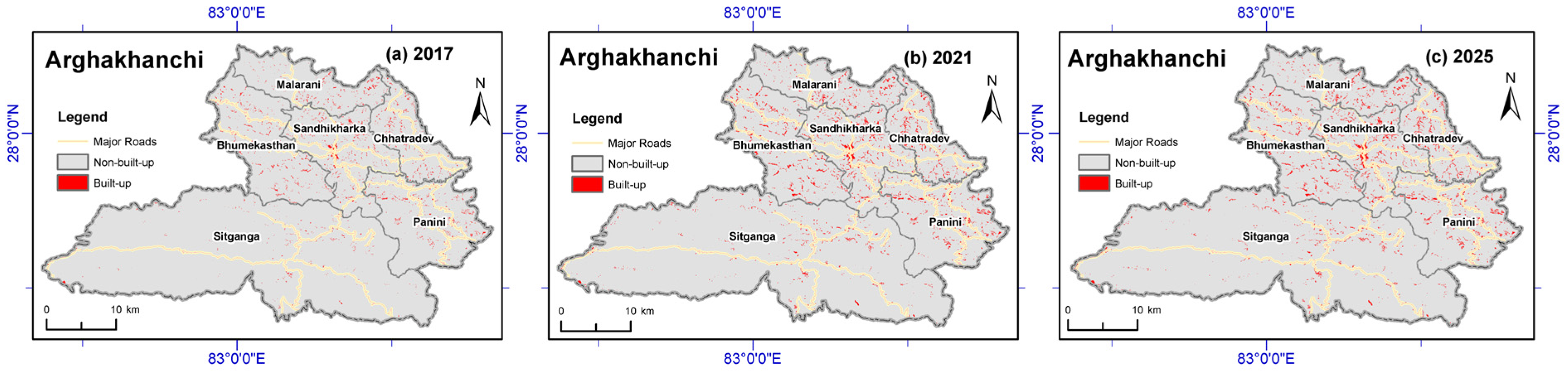
The spatial distribution of built-up expansion shows a dispersed pattern of development rather than concentration around a single urban center (Figure 3). Expansion occurred across multiple settlement clusters, particularly around existing municipal centers, roadside settlements, and valley-bottom inhabited areas. The mapped pattern was characterized by the outward expansion of existing settlements together with the gradual emergence of new built-up patches in previously non-built-up locations.

The largest annual built-up expansion in Arghakhanchi occurred between 2017 and 2018, amounting to 933.56 ha. Annual expansion was smaller during the subsequent years, ranging from 18.61 ha to 419.15 ha (Table 3).

Overall, the results indicate that Arghakhanchi experienced substantial and spatially dispersed built-up expansion during 2017–2025, cumulative built-up extent more than doubling relative to the 2017 baseline.

3.3. Built-Up Expansion in Lalitpur

Lalitpur District experienced substantial built-up expansion between 2017 and 2025 (Table 3). The cumulative built-up extent increased from 3367.43 ha in 2017 to 5583.39 ha in 2025, representing an expansion of 2215.96 ha and an overall increase of approximately 65.8%. The mapped expansion indicates a substantial transformation of the district’s built-up landscape during the study period.

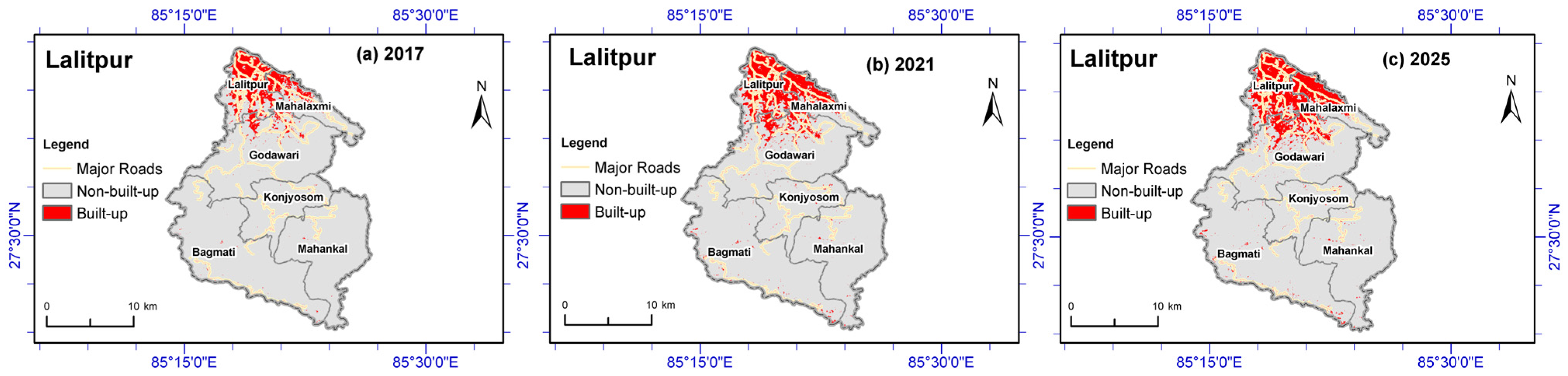
The spatial pattern of built-up expansion shows outward extension from the existing metropolitan core into surrounding peri-urban and semi-rural areas (Figure 4). Most newly developed built-up land emerged around established urban settlements and along major development corridors, leading to the enlargement and gradual merging of previously separated built-up patches. As a result, the mapped built-up extent expanded beyond its traditional boundaries and increasingly occupied adjacent non-built-up land.

Annual built-up expansion showed moderate year-to-year variability, with the largest expansion occurring between 2018 and 2019, when the built-up extent increased by 664.56 ha. Thereafter, annual expansion was generally lower, ranging from 98.61 ha to 284.79 ha between 2020 and 2025. This pattern indicates that the magnitude of annual expansion slowed following the substantial increase observed during the earlier period.

Overall, the results demonstrate that Lalitpur underwent substantial and spatially concentrated built-up expansion during 2017–2025. Unlike the dispersed settlement expansion observed in Arghakhanchi, the mapped pattern in Lalitpur was characterized primarily by the outward extension of existing urban areas, resulting in a more contiguous and consolidated built-up pattern.

3.4. Built-Up Expansion in Chitwan

Among the three study districts, Chitwan experienced the most extensive built-up expansion during the study period (2017–2025) (Table 3). The cumulative built-up extent increased from 8110.96 ha in 2017 to 16,165.61 ha in 2025, representing an expansion of 8054.65 ha and an overall increase of approximately 99.3%. As a result, the district’s built-up extent nearly doubled over the nine-year period, indicating the large magnitude of built-up expansion in the Inner Terai region.

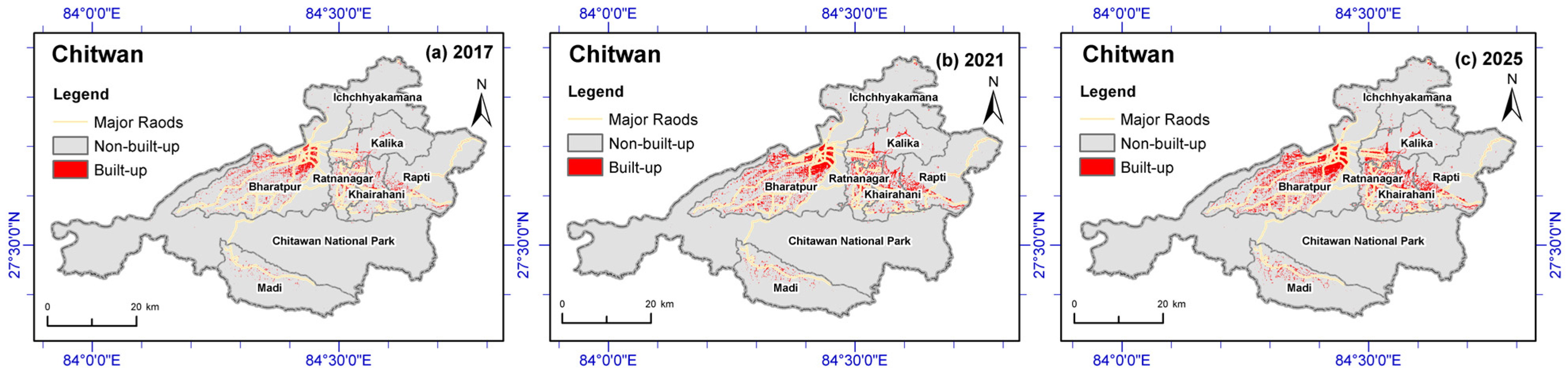
The spatial distribution of built-up expansion shows widespread expansion around existing urban centers and major development corridors (Figure 5). New built-up areas were mapped across large portions of the district, resulting in the enlargement, infilling, and gradual consolidation of existing urban clusters. In contrast to the more dispersed settlement pattern observed in Arghakhanchi and the metropolitan fringe expansion evident in Lalitpur, built-up expansion in Chitwan was characterized by larger, more contiguous built-up patches and extensive corridor-oriented development. The mapped pattern also shows the prominence of major urban centers and development corridors within the district.

Annual built-up expansion varied in magnitude throughout the study period. The largest expansion occurred between 2020 and 2021, when the built-up extent increased by 1487.53 ha. Substantial expansion was also recorded between 2018 and 2019 (1448.17 ha) and between 2019 and 2020 (1287.90 ha). Annual expansion was smaller after 2022, ranging from 425.10 ha to 552.75 ha between 2023 and 2025 (as illustrated in Table 3).

Overall, Chitwan recorded both the largest absolute built-up expansion and the greatest cumulative built-up extent among the three study districts. By 2025, more than 16,000 ha had been included in the cumulative built-up extent, underscoring the scale of mapped transformation in the district. The mapped pattern was characterized by expansion and consolidation along major settlement corridors and urban centers.

3.5. Comparative Built-Up Expansion Dynamics

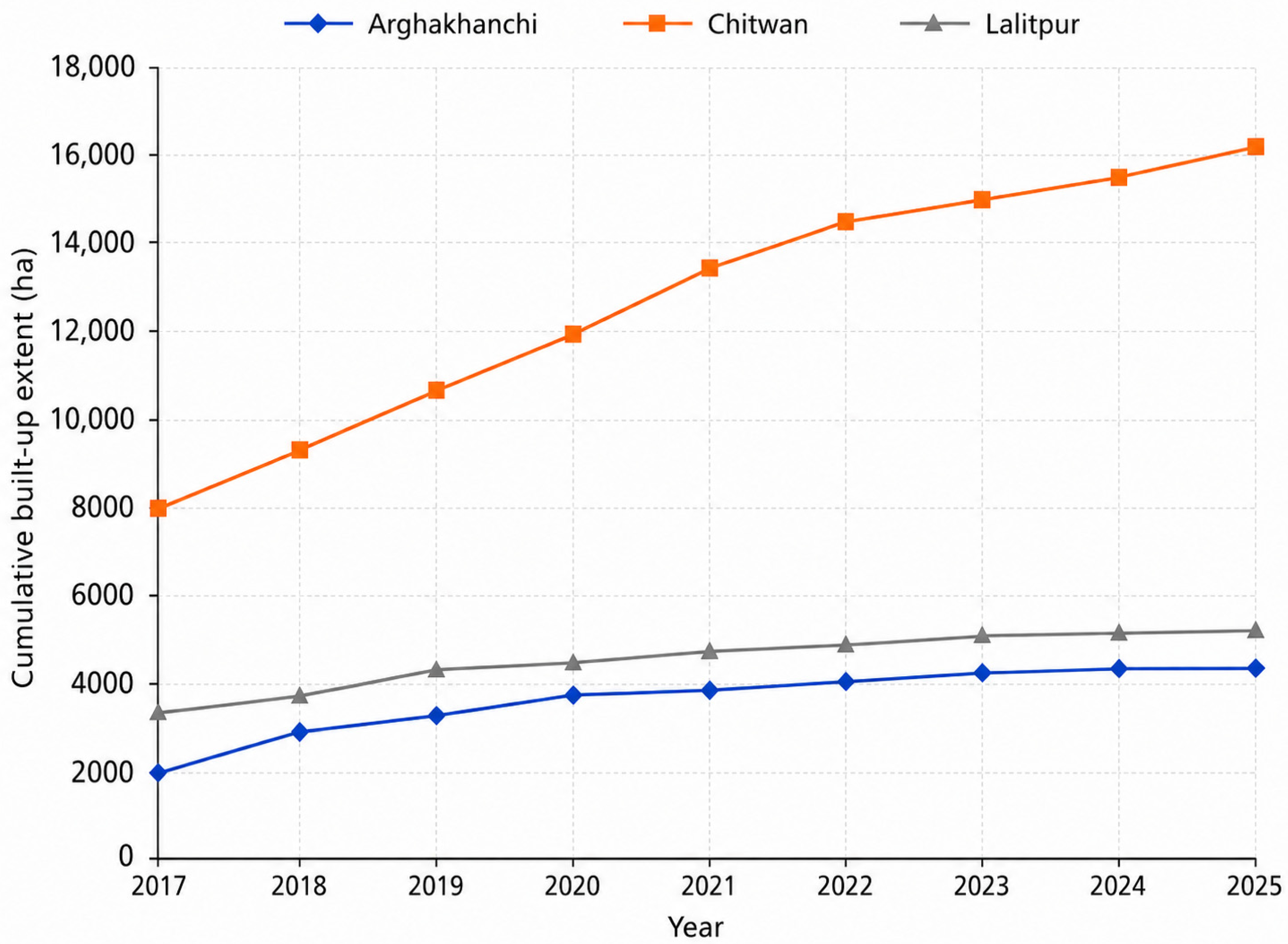
The comparative analysis reveals marked differences in the scale, rate, and spatial characteristics of built-up expansion among the three study districts during 2017–2025 (Table 3; Figure 6). Although all districts experienced a continuous increase in cumulative built-up extent, the magnitude and pattern of expansion varied considerably, reflecting the diverse physiographic settings of Nepal.

In terms of absolute expansion, Chitwan experienced by far the largest increase in cumulative built-up extent. The district’s built-up extent increased from 8110.96 ha in 2017 to 16,165.61 ha in 2025, resulting in a total expansion of 8054.65 ha. This increase was more than three times greater than those observed in Arghakhanchi or Lalitpur. Over the same period, Arghakhanchi and Lalitpur recorded built-up expansions of 2406.20 ha and 2215.96 ha, respectively.

A different pattern emerges when expansion is assessed in relative terms. Arghakhanchi recorded the highest proportional increase, with cumulative built-up extent expanding by approximately 117.6% during the study period. Chitwan followed with an overall increase of 99.3%, while Lalitpur exhibited the lowest relative increase at 65.8%. These findings suggest that districts with comparatively small initial built-up extents can experience rapid proportional expansion even when their absolute increase in built-up extent is more modest.

To facilitate comparison among the study districts, key built-up expansion indicators derived from the cumulative built-up extent statistics are summarized in

Table 4. Summary of built-up expansion statistics in Arghakhanchi, Lalitpur, and Chitwan districts, 2017–2025.

District	Cumulative Extent 2017 (ha)	Cumulative Extent 2025 (ha)	Total Expansion (ha)	Increase Relative to 2017 (%)
Arghakhanchi	2045.93	4452.13	2406.20	117.6
Lalitpur	3367.43	5583.39	2215.96	65.8
Chitwan	8110.96	16,165.61	8054.65	99.3

. The table presents the initial and final built-up extents, total built-up expansion, and overall growth rates for each district during the 2017–2025 study period. These summary statistics provide a concise overview of the magnitude and relative scale of built-up expansion across the contrasting physiographic settings.

The temporal evolution of built-up expansion also differed across the study districts (Figure 6). Arghakhanchi experienced a sharp expansion during the early years of the study period, particularly between 2017 and 2018, after which annual expansion was generally smaller. Lalitpur showed moderate year-to-year variability, with the most substantial expansion occurring between 2018 and 2019, and generally smaller annual expansion thereafter. In contrast, Chitwan recorded comparatively large annual expansion during the earlier and middle years, with annual expansion exceeding 1000 ha between 2018 and 2022, followed by smaller values during 2023–2025.

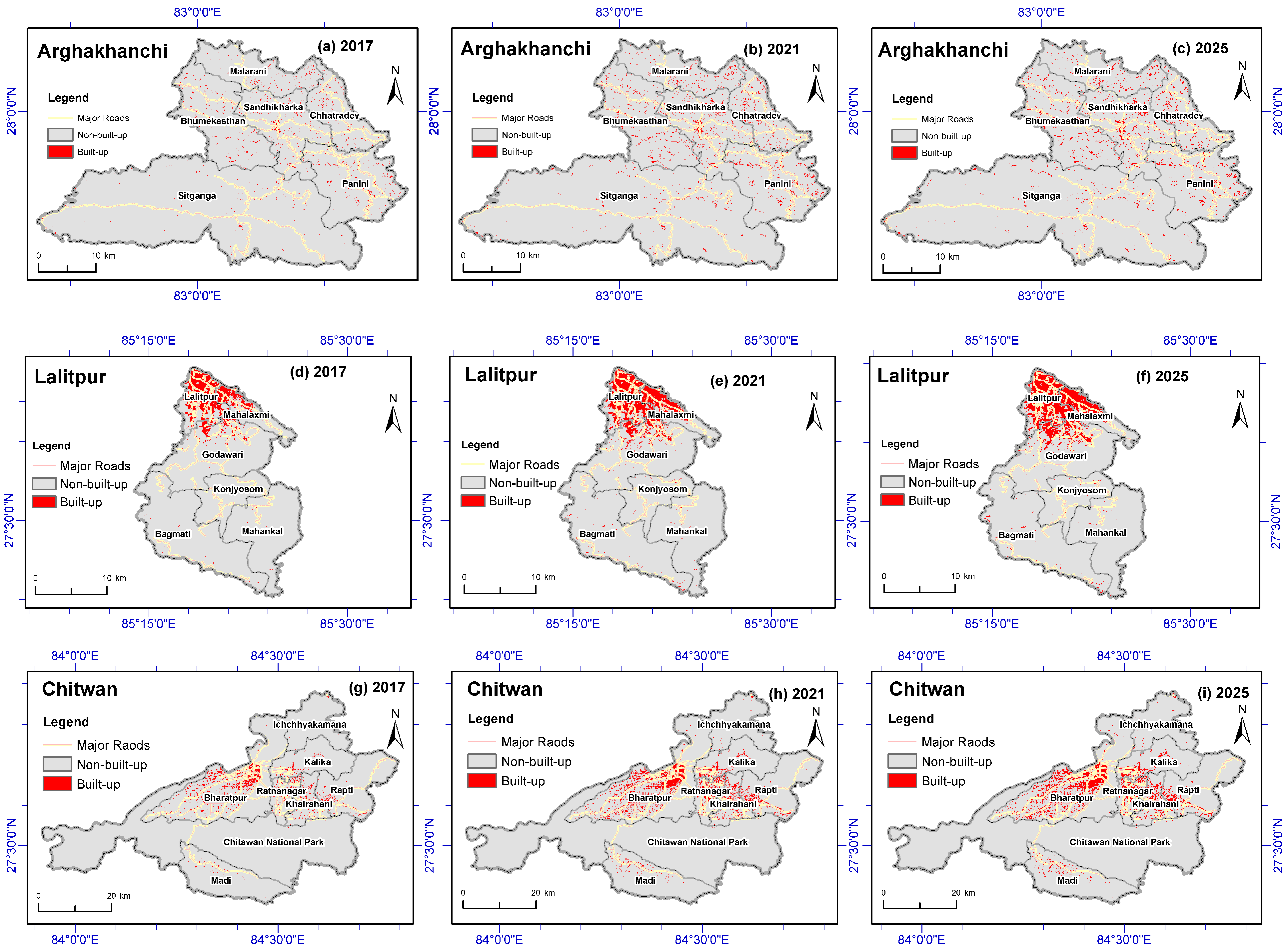
Distinct spatial patterns of built-up expansion further differentiate the three districts (Figure 7). In Arghakhanchi, built-up expansion was dispersed across numerous small settlement clusters, consistent with the district’s hill-settlement structure and fragmented topography. Lalitpur exhibited a more consolidated pattern characterized by the outward expansion of existing urban areas and the gradual merging of adjacent built-up zones. Chitwan, on the other hand, displayed extensive and spatially contiguous built-up expansion, with large built-up patches expanding along major settlement and transportation corridors across the district.

Overall, the comparative results demonstrate that built-up expansion occurred across all three physiographic settings of Nepal during 2017–2025, but with substantially different magnitudes and spatial expressions. Arghakhanchi experienced the highest proportional increase, Lalitpur underwent spatially concentrated metropolitan and peri-urban expansion, and Chitwan recorded the largest absolute increase in built-up extent. Together, these findings underscore the spatial heterogeneity of built-up expansion patterns in Nepal and highlight the importance of considering local geographic and settlement characteristics when assessing built-up expansion dynamics.

3.6. Baseline Comparison and Sensitivity Analysis

The diagnostic comparison conducted for Lalitpur in 2025 showed clear differences among the tested predictor configurations (

Table 5. Diagnostic baseline/component comparison and threshold-sensitivity results for Lalitpur, 2025 (n = 231 common labelled observations).

Analysis	Configuration/Setting	OA (%)	PA (%)	UA (%)	F1 (%)	Kappa
Baseline/component comparison	B0: Sentinel-2 bands	86.6	70.1	81.0	75.2	0.66
	B1: B0 + spectral indices	85.7	70.1	78.3	74.0	0.64
	B2: B1 + Dynamic World + DEM + slope	91.8	76.1	94.4	84.3	0.79
	Dynamic World standalone	80.5	77.6	63.4	69.8	0.56
Probability sensitivity	0.45; slope = 35°	87.4	71.6	82.8	76.8	0.68
	0.50; slope = 35° (adopted)	89.2	68.7	92.0	78.6	0.72
	0.55; slope = 35°	88.7	64.2	95.6	76.8	0.70
Slope sensitivity	30°; probability = 0.50	88.7	67.2	91.8	77.6	0.70
	35°; probability = 0.50 (adopted)	89.2	68.7	92.0	78.6	0.72
	40°; probability = 0.50	89.6	70.1	92.2	79.7	0.73

Note: B0–B2 evaluate predictor composition using RF class predictions, whereas the sensitivity analysis evaluates probability-based classification with the stated NDVI, MNDWI, probability, and slope constraints. The diagnostic cross-validation results are therefore intended for within-analysis methodological comparison and are separate from the independent validation results reported in Table 2.

). The Sentinel-2 baseline (B0) achieved an OA of 86.6% and a built-up F1-score of 75.2%. The addition of the four spectral indices alone (B1) did not improve performance, yielding an OA of 85.7% and an F1-score of 74%. In contrast, the combined predictor configuration incorporating Sentinel-2 bands, spectral indices, Dynamic World built-up probability, elevation, and slope (B2) achieved the highest performance, with an OA of 91.8%, a built-up F1-score of 84.3%, and a Kappa coefficient of 0.79. The standalone Dynamic World benchmark produced lower overall performance, with an OA of 80.5% and an F1-score of 69.8%. The B2 configuration also showed substantially higher built-up User’s Accuracy (94.4%), indicating fewer commission errors than the simpler configurations and standalone Dynamic World.

The focused sensitivity analysis indicated comparatively modest changes in classification performance within the tested parameter ranges. Varying the RF built-up probability threshold between 0.45 and 0.55 produced OA values ranging from 87.4% to 89.2% and F1-scores ranging from 76.8% to 78.6%. Similarly, changing the Lalitpur slope threshold between 30° and 40° resulted in OA values of 88.7–89.6% and F1-scores of 77.6–79.7%. The probability-threshold results also showed the expected trade-off between omission and commission errors, with higher thresholds increasing User’s Accuracy while reducing Producer’s Accuracy. Although the adopted settings were not uniquely optimal within every tested performance metric, the relatively limited variation across the tested ranges indicates that the diagnostic results were not highly sensitive to moderate changes in these two thresholds. Because this analysis was based on cross-validation of the manually labelled training features rather than the independent validation sample (n), the results should be interpreted as relative methodological evidence and do not replace the accuracy assessment reported in Table 2.

4. Discussion

The findings reveal substantial built-up expansion across all three study districts between 2017 and 2025, although the scale, spatial form, and temporal patterns of expansion differed considerably among the contrasting physiographic settings of Nepal. These variations highlight the geographically differentiated nature of built-up expansion across the study districts. Beyond quantifying built-up expansion, the study also assessed the performance of a multi-product and terrain-informed classification and accumulation workflow that combined multispectral satellite imagery, probabilistic land-cover products, terrain variables, Random Forest classification, and cumulative built-up expansion mapping. The results provide an opportunity to examine both the performance and methodological implications of the implemented approach and the broader geographic context associated with built-up expansion in different environments. The following sections discuss the performance of the classification framework, built-up expansion patterns across contrasting physiographic settings, the interpretation and implications of cumulative built-up expansion mapping, and the limitations and potential applications of the proposed methodology.

4.1. Performance of the Hybrid Multi-Product and Terrain-Informed Workflow

The classification results suggest that the proposed hybrid multi-product and terrain-informed workflow performed well in mapping built-up areas across Nepal’s diverse physiographic settings. Overall Accuracy (OA) values ranging from 86.4% to 92.4%, built-up F1-scores from 84.7% to 91.3%, and Kappa coefficients between 0.81 and 0.91 indicate strong agreement between the classified outputs and the reference data. These accuracy levels are within the range of those reported in recent urban land-cover mapping studies that have used machine learning techniques and cloud-based remote sensing platforms [27,32,61].

The workflow integrated complementary geospatial products and predictor variables. Sentinel-2 imagery provided detailed multispectral information for distinguishing urban land cover, while Dynamic World built-up probability layers supplied additional probabilistic information for built-up classification. ESRI Global Land Cover was used separately as an auxiliary comparison and visual-calibration product. The inclusion of spectral indices such as NDVI, NDBI, MNDWI, and BSI supported the discrimination of built-up land from vegetation, water bodies, and exposed or sparsely vegetated surfaces that often exhibit similar spectral characteristics.

Terrain-related variables were incorporated to account for terrain-related classification challenges across physiographically heterogeneous landscapes. Elevation and slope information derived from the SRTM Digital Elevation Model provided information on topographic influences that commonly affect land-cover classification, including steep terrain, shadow effects, and spectral variability associated with complex hill environments. Their inclusion is particularly relevant in Nepal, where fragmented settlement patterns and rugged terrain often limit the effectiveness of conventional urban mapping approaches.

The use of the Random Forest algorithm provided a suitable machine-learning basis for the classification workflow. Its ability to accommodate large numbers of predictor variables, model complex non-linear relationships, and perform well with heterogeneous training data has been widely demonstrated in land-cover classification studies [12,13]. In this study, the combination of multiple predictor layers within the Random Forest framework supported built-up classification across districts characterized by markedly different environmental and settlement conditions.

The additional Lalitpur diagnostic analysis provides focused evidence on the relative performance of the predictor configuration. The combined B2 configuration achieved an OA of 91.8% and a built-up F1-score of 84.3%, compared with 86.6% and 75.2%, respectively, for the Sentinel-2 baseline (B0) and 80.5% and 69.8% for standalone Dynamic World. The spectral-index configuration (B1) alone did not improve performance relative to the Sentinel-2 baseline, suggesting that the observed improvement was associated with the combined multi-product and terrain-derived information rather than to the addition of every predictor group individually. The focused sensitivity analysis further showed only modest changes in OA and F1 across the tested RF probability and slope thresholds. These diagnostic results should nevertheless be interpreted cautiously because they were derived from the 2025 Lalitpur training features under cross-validation and were intended to complement, rather than replace, the independent validation results reported in Table 2.

The cumulative component of the workflow and its interpretive implications and limitations are discussed in Section 4.3.

4.2. Built-Up Expansion Across Contrasting Physiographic Settings

The comparative analysis highlights marked differences in the scale, spatial form, and trajectory of built-up expansion across the study districts. Although all three districts experienced substantial built-up expansion between 2017 and 2025, the nature of that expansion varied considerably across settings characterized by differences in topography, settlement structure, accessibility, and regional development processes. These findings suggest that the mapped expansion patterns should be interpreted in relation to their contrasting physiographic and settlement contexts.

Arghakhanchi, located in Nepal’s mid-hill region, displayed a dispersed pattern of built-up expansion, with expansion occurring through the gradual enlargement of existing market centers, roadside settlements, and small settlement clusters. The district’s rugged terrain, steep slopes, and fragmented settlement structure are consistent with the observed spatially scattered expansion pattern. Previous studies of hill urbanization in Nepal have similarly associated settlement expansion with road connectivity and emerging municipal centres [28,30]. Although Arghakhanchi recorded a smaller absolute increase in built-up extent than Chitwan, it achieved the highest proportional increase among the study districts, indicating substantial expansion from a relatively modest built-up base.

A markedly different pattern was evident in Lalitpur. As part of the Kathmandu Valley metropolitan region, built-up expansion largely occurred through the outward spread of existing built-up areas into surrounding peri-urban landscapes. Expansion was accompanied by increasing connectivity among built-up patches. This pattern is consistent with previous research documenting peri-urbanization and urban sprawl in the Kathmandu Valley and discussing population growth, infrastructure investment, and metropolitan expansion as important contextual factors [20,21,27]. Compared with the other districts, Lalitpur exhibited a lower proportional increase, largely because a substantial built-up extent already existed at the beginning of the study period.

Chitwan experienced the most extensive built-up expansion among the three districts, recording both the largest absolute increase in built-up extent and the broadest spatial extent of expansion. The mapped expansion occurred through the expansion and consolidation of large built-up clusters, particularly along major transportation corridors and around established urban centers. Unlike predominantly hill settings, the relatively flat terrain of the Inner Terai presents fewer topographical constraints and is consistent with the broader spatial expansion observed across the district. In the mapped results, built-up expansion was observed over much larger areas and at a greater magnitude than in either Arghakhanchi or Lalitpur. Comparable corridor-oriented development patterns have been reported in rapidly urbanizing lowland regions and discussed in relation to transportation infrastructure, market accessibility, and regional economic integration [2,5].

Taken together, these patterns show that built-up expansion differed considerably among the three study settings. The observed differences are consistent with contrasting physiographic, settlement, and regional development contexts. In hill settings, the mapped pattern was fragmented and dispersed across multiple settlement nodes. The metropolitan peri-urban setting showed outward expansion and increasing built-up consolidation, while the Inner Terai setting exhibited large-scale and spatially contiguous expansion along development corridors. These differences underscore the importance of incorporating physiographic context into built-up monitoring frameworks, land-use planning, and sustainable development strategies. More broadly, the findings suggest that approaches to managing built-up expansion should be tailored to the distinct geographic and settlement characteristics of different regions rather than relying on a single planning model.

4.3. Implications of Cumulative Built-Up Expansion Mapping

A key methodological contribution of this study is the incorporation of a cumulative mapping procedure for long-term built-up expansion analysis. While recent advances in machine learning, cloud computing, and Earth observation data have significantly enhanced land-cover classification, maintaining temporal consistency across annual datasets remains a persistent challenge. Built-up areas identified in one year may disappear in subsequent classifications, not because of actual land-cover change, but due to atmospheric variability, seasonal differences, mixed-pixel effects, classification uncertainty, or inconsistencies in training data [24,25]. Such fluctuations can complicate the interpretation of long-term expansion patterns.

The cumulative mapping procedure adopted in this study was designed to address this issue by introducing a simple temporal logic into the expansion analysis. Once a pixel was identified as built-up, it was retained as built-up in subsequent years. By retaining earlier detections, the procedure provided a continuous representation of the progressively detected built-up extent.

This consideration is particularly evident in Arghakhanchi, where built-up development is distributed across numerous small and fragmented settlement clusters. In such environments, relatively minor spectral differences between annual images can lead to substantial classification instability, causing built-up areas to appear and disappear from one year to the next. The cumulative procedure limits such apparent disappearance by retaining previously detected built-up locations and thereby facilitates interpretation of progressive spatial expansion

Beyond its methodological role, cumulative built-up expansion mapping can provide a useful spatial record for land-use planning, infrastructure investment, environmental management, disaster-risk reduction, and urban governance. For such applications, the cumulative extent provides a straightforward representation of where built-up development had been detected by successive years.

At the same time, the approach is not without limitations. Because previously detected built-up pixels were retained in subsequent cumulative outputs, the procedure does not capture demolition, restoration, disaster-related land-cover change, or temporary built-up conditions. Consequently, the method may overestimate the persistence of built-up land where such reversals occur. This trade-off reflects a broader balance between temporal stability and sensitivity to rarely occurring built-up land-cover reversals.

Overall, the cumulative approach provides an interpretable representation of progressively detected built-up expansion through time, but it should be distinguished from bidirectional land-cover change analysis and should not be interpreted as evidence of uninterrupted annual growth.

4.4. Limitations and Future Research

Although the multi-product and terrain-informed workflow produced satisfactory classification accuracy, several limitations should be considered when interpreting the results. The first relates to the spatial resolution of the input imagery. Although Sentinel-2 provides valuable multispectral information at a 10–20 m spatial resolution for the bands used in this study, mixed-pixel effects remain unavoidable in fragmented settlement environments, narrow transportation corridors, dispersed rural housing clusters, and peri-urban transition zones. This challenge is particularly pronounced in rugged and heterogeneous landscapes, where settlement patterns are often highly heterogeneous and may occur at spatial scales smaller than the sensor resolution [8,64]. In addition, the use of scene-level cloud filtering without a separate pixel-level cloud and cloud-shadow mask may leave some residual atmospheric contamination in the annual composites.

A second limitation concerns the spectral complexity of certain land-cover types. Despite the integration of Dynamic World probability layers, spectral indices, and terrain variables, some environments remain difficult to classify accurately. Exposed riverbeds, quarry sites, barren slopes, construction areas, and dry agricultural fields can exhibit spectral responses similar to built-up surfaces, increasing the potential for classification ambiguity [33,65]. NDVI suppression, MNDWI filtering, terrain constraints, and connected-pixel filtering were applied to limit these errors; however, a degree of residual misclassification is likely to remain in spectrally complex landscapes.

Another consideration relates to the validation process. Accuracy assessment was primarily based on stratified sampling of 300 validation points for each district in each of the three selected years (2017, 2021, and 2025), together with visual interpretation of high-resolution imagery. While these methods are widely accepted and commonly applied in remote sensing research, some uncertainty inevitably remains, particularly for historical years where reference imagery is limited or of lower quality [56,66]. Consequently, the reported accuracy measures should be interpreted within the constraints of the available reference data.

These limitations also point to several promising directions for future research. Built-up expansion monitoring could be further improved through the use of higher-resolution satellite imagery, deep learning-based classification approaches, and more advanced spatiotemporal modelling techniques. Future studies may also benefit from integrating remote sensing products with cadastral records, land transaction data, transportation networks, real estate indicators, and other socioeconomic datasets. Such integration would allow researchers to move beyond mapping where built-up expansion occurs and provide deeper insight into the processes and drivers that shape urban development.

The additional diagnostic analysis provided a focused assessment of predictor composition and selected classification thresholds. However, its scope was limited to Lalitpur in 2025 and did not evaluate all post-classification components or the full range of physiographic settings represented in the study. Future work could extend component-wise and sensitivity analyses across additional districts and assessment years and incorporate variable-importance assessment and broader parameter testing. Such analyses would help determine whether the relative contributions observed in the Lalitpur diagnostic case remain consistent across different geographic, environmental and settlement conditions.

In the context of Nepal, an important next step is to evaluate the transferability of the proposed workflow across larger geographic areas and diverse environmental settings. Assessing its performance at regional and national scales would help determine its broader applicability for operational built-up expansion monitoring. More broadly, the integration of multi-product remote sensing data with socioeconomic data and sustainable development indicator has considerable potential to support sustainable urban planning, land management, and evidence-based policy development in increasingly dynamic urban environments.

5. Conclusions

This study developed and applied an integrated multi-product and terrain-informed workflow for mapping built-up expansion across three contrasting physiographic settings of Nepal from 2017 to 2025. The workflow combined Sentinel-2 spectral information and derived indices, Dynamic World built-up probabilities, SRTM-derived terrain variables, district-specific Random Forest classification, and post-classification constraints to generate preliminary yearly built-up detections, which were subsequently integrated through cumulative expansion mapping. The classification achieved overall accuracy values of 86.4% to 92.4%, built-up F1-scores of 84.7% to 91.3%, and Kappa coefficients between 0.81 and 0.91 demonstrating the effectiveness of the approach across diverse geographic settings.

Substantial differences in both the magnitude and spatial characteristics of built-up expansion were observed among the three districts. Chitwan recorded the largest absolute expansion, with cumulative built-up extent increasing by 8054.65 ha between 2017 and 2025, while Arghakhanchi showed the highest proportional increase at 117.6%, reflecting expansion from a comparatively smaller 2017 baseline. Lalitpur recorded an increase of 2215.96 ha, (65.8%) and exhibited a more spatially concentrated peri-urban development pattern. The mapped expansion was comparatively dispersed in Arghakhanchi, concentrated around the metropolitan and peri-urban areas in Lalitpur, and broader and corridor-oriented in Chitwan, demonstrating contrasting expressions of built-up expansion across Nepal’s mid-hill, metropolitan peri-urban, and Inner Terai settings.

The principal methodological contribution of the study is the integration of district-specific hybrid built-up classification with cumulative expansion mapping and its comparative implementation across contrasting physiographic settings. The cumulative approach provides a consistent representation of the progressive spatial extent detected as built-up and enables annual built-up expansion to be quantified from successive cumulative extents. However, because previously detected built-up locations are retained in subsequent years, the method does not represent demolition, abandonment, restoration, or other reversals and should not be interpreted as net annual land-cover change. The proposed workflow therefore provides a practical approach for comparative built-up expansion monitoring across heterogeneous landscapes. The additional 2025 Lalitpur diagnostic analysis further supported the value of the combined predictor configuration relative to the simpler Sentinel-2 baseline and standalone Dynamic World and indicated comparatively modest performance variation across the tested RF probability and slope thresholds. Broader component-wise assessment across additional districts, years, and physiographic settings remains an important direction for future research.