Article

Evidence Admission in Spatial Decision Models: Gating Layers Before Fusion in Municipal Seismic Screening

GIS Center, Faculty of Engineering, University of Balamand, Koura 1352, Lebanon
*
Author to whom correspondence should be addressed.
ISPRS Int. J. Geo-Inf. 2026, 15(9), 425; https://doi.org/10.3390/ijgi15090425
Submission received: 29 July 2026 / Revised: 13 September 2026 / Accepted: 15 September 2026 / Published: 17 September 2026

Abstract

Seismic geospatial decision models can produce misleading outputs without rigorous input validation. Fusion conceals the defect: weight-sensitivity testing on an inadmissible layer reports stability rather than validity. This paper presents Evidence-Gated Screening (EGS), a four-gate framework. It tests computational provenance, applicability, decision-relevant signal, and input support before fusion. EGS audited six candidates for 1552 building footprints in Aabadiyeh, Lebanon: a construction-epoch proxy, two soil products, an exploratory Age-Soil Index, a Newmark displacement raster, and an Earthquake Risk Index. Only the proxy was conditionally admitted. Two interpreters validated it on a stratified probability sample of 216 buildings, giving binary accuracies of 0.833 (0.782–0.880) and 0.861 (0.815–0.907), with κ = 0.832 on the image evidence. The remaining candidates were rejected, including the risk index. Of 87,492 evaluable cells, 56.30% fell outside the stated critical-acceleration domain; raster-to-building transfer omitted 270 footprints. Gating returned a queue of 400 buildings and not the composite’s 303. Four products were assessed by two independent assessors, who agreed on 13 of 16 gates and on all four dispositions: two were conditionally admitted, two rejected. This indicates that EGS can screen out inadmissible inputs before fusion and support building inspection prioritization, but not vulnerability prediction without building-level validation.

1. Introduction

Municipal earthquake-risk reduction often begins with a practical allocation problem: which buildings should be inspected first when detailed structural records are unavailable? Building-specific assessment requires information on structural systems, materials, detailing, occupancy, maintenance, alterations, retrofit history, and local ground conditions. Municipal inventories rarely contain all of these attributes. Geographic information systems (GIS) can organize incomplete observations and proxies into a preliminary screening workflow, but such screening cannot substitute for engineering assessment or predict building-specific performance [1,2,3,4].
GIS screening is valuable precisely because it can bring heterogeneous evidence into a common spatial framework. Remotely sensed observations, building footprints, terrain grids, soil polygons, and model outputs can be aligned and transferred to municipal decision units. That convenience also creates a governance problem. A layer may appear ready for analysis once it has a coordinate reference system and a legend, even when its generating process is undocumented, its spatial support is incompatible with buildings, its values fall outside a calibration domain, or its classes have no independent empirical support.
Multi-criteria decision analysis (MCDA), the Analytic Hierarchy Process (AHP), and weighted overlay are widely used to combine such layers [5,6,7,8,9]. These methods make preferences and weights explicit, which is useful for decision analysis. They do not, by themselves, establish that a candidate layer is scientifically eligible for inclusion. A well-documented weight cannot repair an unsupported proxy, an unreproducible raster, or a transfer operation that silently omits decision units.
Sensitivity and uncertainty analysis address related but different questions. Weight sensitivity asks how an output changes when weights or thresholds change. Uncertainty analysis characterizes the consequences of uncertainty in inputs, parameters, or model form [10]. Neither test demonstrates that an input is applicable to the stated decision, that its decision-relevant class contains valid signal, or that its empirical interpretation is supported. Eligibility must be evaluated before parameter perturbation can be meaningfully interpreted.
Spatial data-quality standards and fitness-for-use research provide the conceptual foundation for this evaluation. International Organization for Standardization (ISO) 19157-1 describes data-quality components and evaluation principles [11]. Fitness-for-use research asks whether quality is adequate for a particular task, not whether a dataset is good in general [12,13]. Provenance models document entities, activities, and agents [14], while reproducible GIS research emphasizes recoverable environments, operations, inputs, and outputs [15,16,17,18,19]. Metadata is necessary for these tasks, but metadata alone does not make an admission decision [20].
Composite indices are also used outside seismic screening. For example, desertification assessments combine reclassified soil, vegetation, climate, and management variables into a common index [21]. These inputs may differ in resolution and require resampling and expert-defined classification thresholds [21]. This raises a broader question: which components are suitable for inclusion before they are combined?
The unresolved problem is therefore not simply how to describe quality or propagate uncertainty. It is how to decide, transparently and before fusion, whether a spatial product may enter a decision model for a specified purpose and analytical unit. Existing weighted-overlay practice often treats every available layer as a candidate for weighting. Data-quality reporting may identify defects without stating their operational consequence. Reproducibility audits may show that a formula can be rerun without establishing whether its inputs are applicable or scientifically supported.
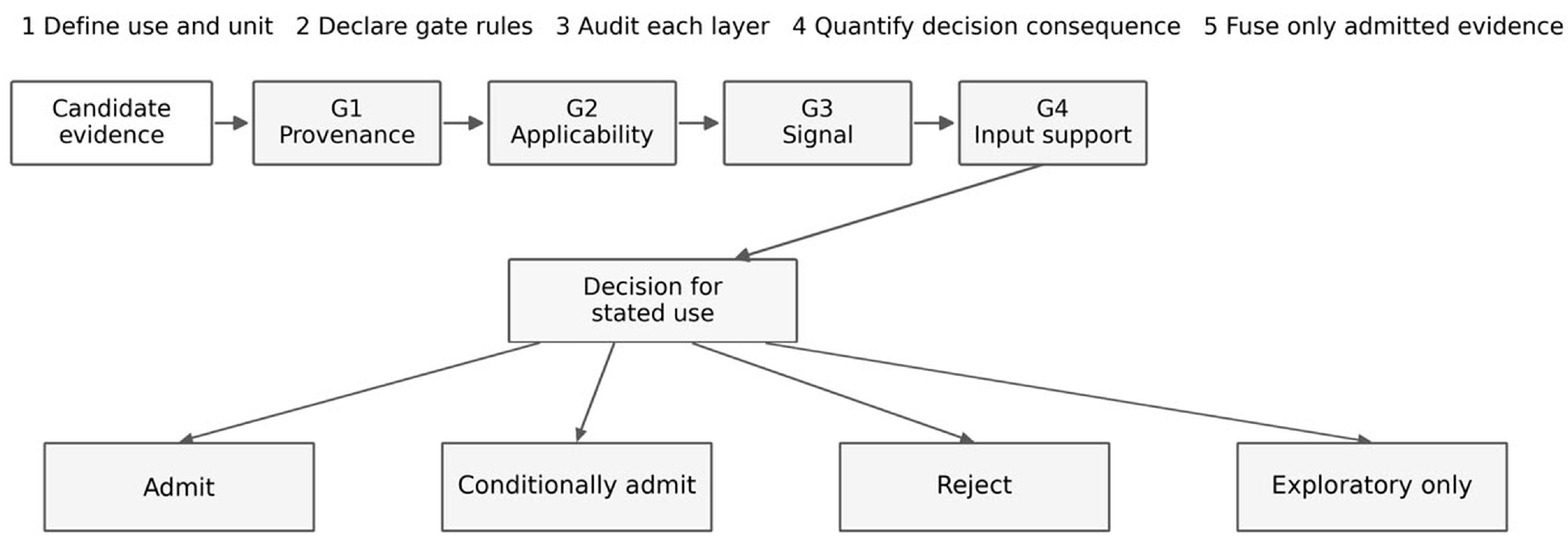
This paper presents Evidence-Gated Screening (EGS) as a structured pre-fusion procedure, evaluated through a municipal seismic-screening case study. EGS is organized around four gates: computational provenance, applicability, signal validity, and input support. EGS does not estimate weights and does not replace validation, uncertainty propagation, or data-quality metadata. It converts evidence about those matters into an explicit, use-specific admission decision. Reproduction is retained as a gate because it is diagnostic. A layer that reproduces and then fails applicability shows where its defect lies: in data meaning or scale, and not in computational execution. Hard failures exclude a layer from fusion; bounded limitations may justify conditional admission for a stated low-consequence use; rejected layers remain visible in the audit record. Throughout this paper, the term “gate” is a rule used to decide whether evidence can be included. EGS does not use machine learning or deep learning.
This study addresses these five questions: (1) Provenance: Can each candidate product be reproduced from documented inputs and operations? (2) Applicability: Is each product applicable to the intended decision, spatial scale, calibration range, and analytical unit? (3) Signal Validity: Does each decision-relevant class contain valid discriminatory signal? (4) Input Support: Are the inputs and proxy interpretations independently supported? (5) Decision Consequences: How do evidence-admission decisions change the resulting municipal inspection queue and its counterfactual alternatives? These questions are examined on 1552 building footprints in Aabadiyeh, Lebanon. The case includes a construction-epoch proxy, two soil products, an exploratory Age-Soil Index (ASI), a Newmark displacement raster, a project-specific raster Earthquake Risk Index (ERI), and a raster-to-building transfer audit. Section 2 defines the framework and audit methods, Section 3 reports the gate evidence in the same order, Section 4 discusses the GIScience implications, and Section 5 states the resulting decision boundaries.

2. Materials and Methods

2.1. Study Area and Decision Units

The municipality of Aabadiyeh is situated in the Baabda District and lies on the western flank of Mount Lebanon, with a total area of 9.16 km2 (Figure 1a). Aabadiyeh is situated within a seismically active region, approximately 25 km west of the Yammouneh Fault, the principal active strand of the Dead Sea Transform Fault (DSTF) system within the Lebanese Restraining Bend (LRB) [22,23].
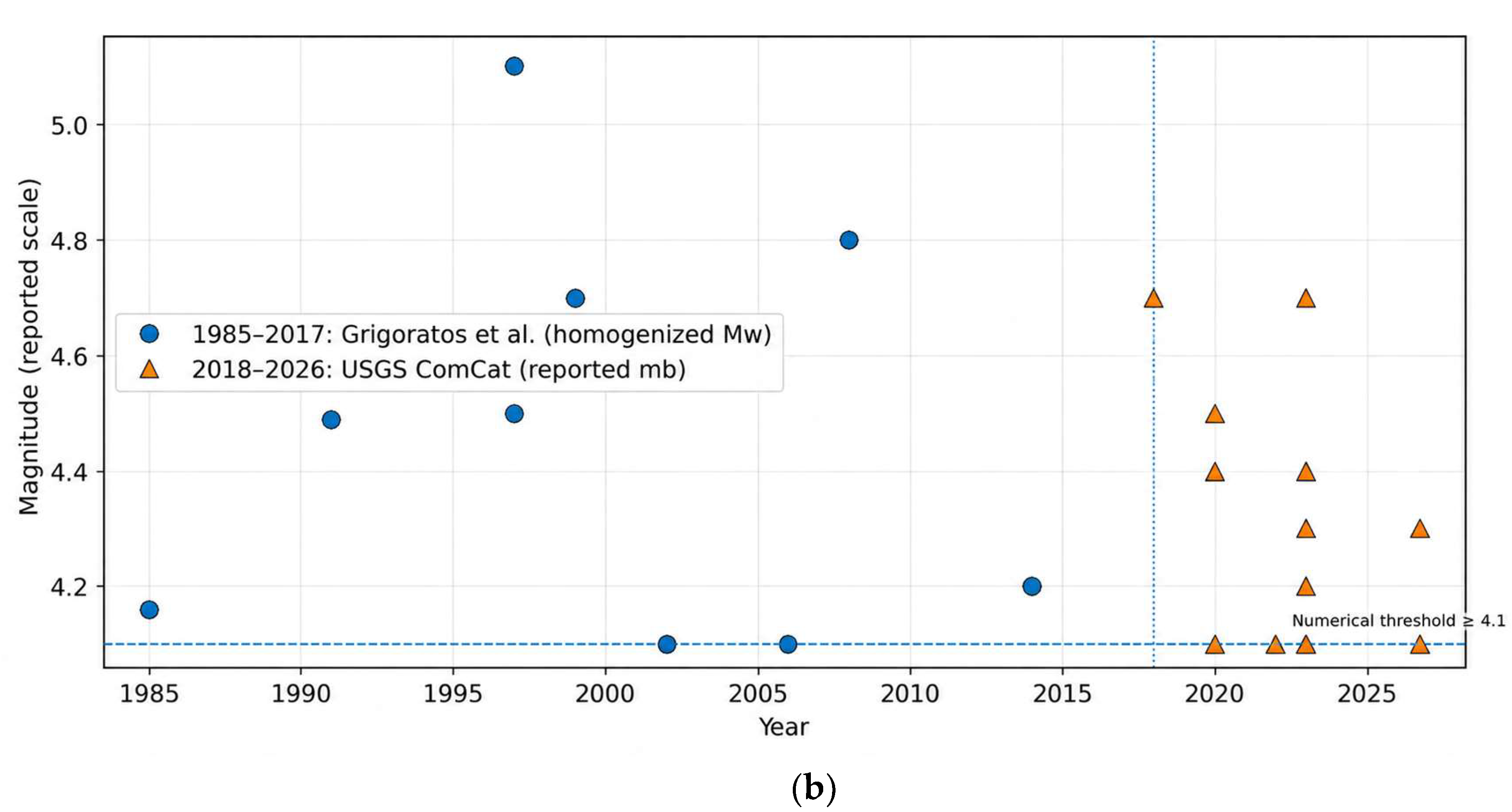
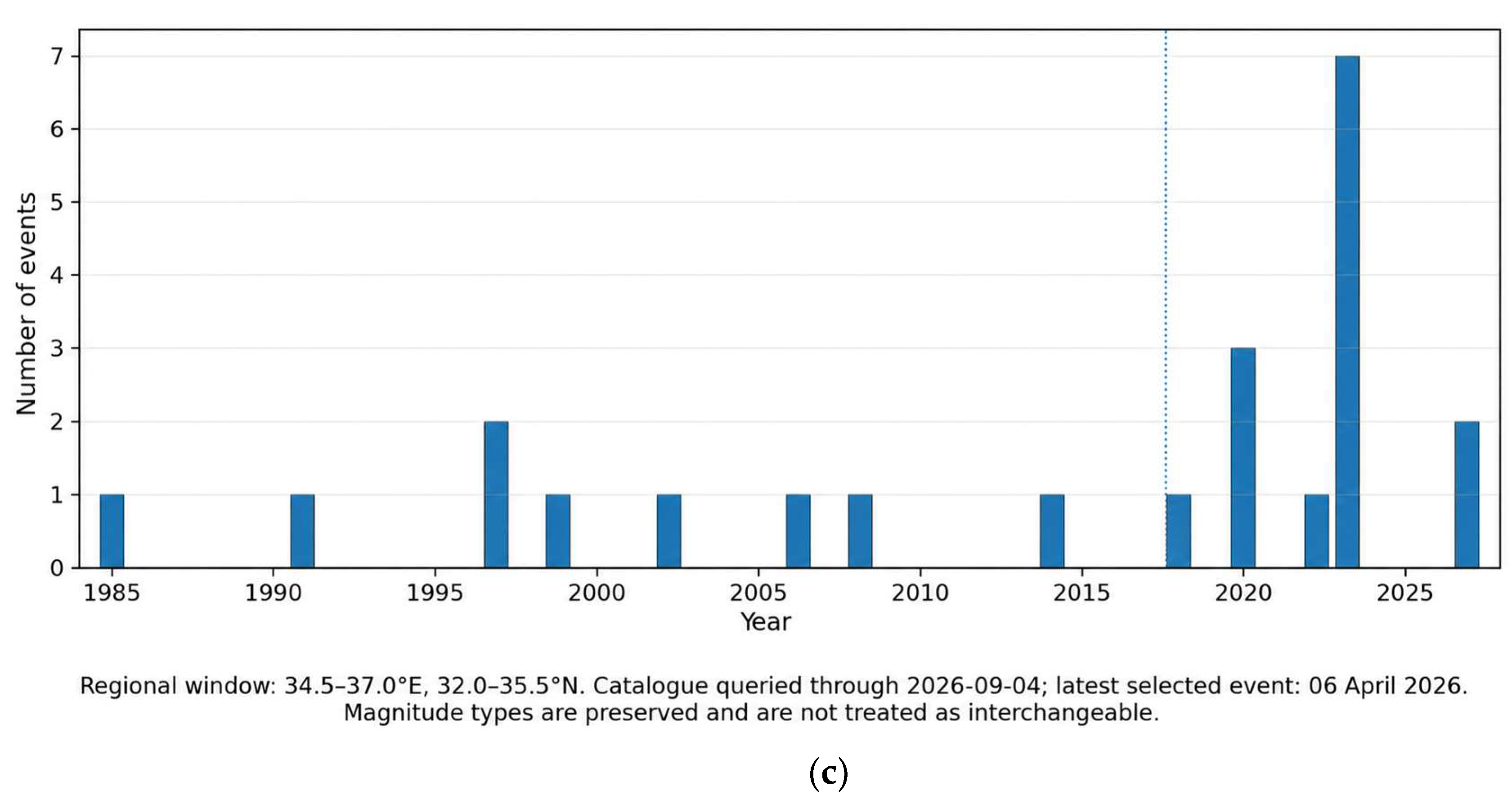
The faults shown in Figure 1a were obtained from the Global Earthquake Model (GEM) Global Active Faults Database [24]. Figure 1b,c show 23 regional earthquakes within 34.5–37.0° E and 32.0–35.5° N, plotted by magnitude through time and by annual count. Only events with a magnitude of 4.1 or greater were included. Events from 1985 to 2017 were obtained from the Grigoratos et al. catalog [25,26] and are reported as moment magnitude (Mw); events from 2018 to 2026 were obtained from United States Geological Survey (USGS) Comprehensive Earthquake Catalog (ComCat) [27] and retain the reported body-wave magnitude (mb). Mw and mb are preserved as reported and were not treated as interchangeable magnitude measures.
Lebanon lies within the Levant Fault System, and active faults in the region are documented sources of substantial seismic hazard. Fault-based probabilistic hazard modeling for Lebanon reports elevated computed hazard levels near the Yammouneh Fault and the wider Levant Fault System [22]. Paleoseismic trenching corroborates this from an independent line of evidence. The fault has produced 10 to 13 surface-rupturing earthquakes over the past 12,000 years, and these earthquakes cluster in time rather than recurring at simple fixed intervals [23]. This combination of computed hazard and a long, clustered rupture history motivate the present screening approach. The interval between major ruptures can exceed the length of the instrumental record itself. Inspection priorities cannot rely on recent seismicity alone, and must instead draw on building-level evidence collected between events.
The decision unit is the unit at which the decision is made and recorded. Here, it was the municipal building footprint, represented by 1552 polygons. Vector analyses used World Geodetic System 1984 (WGS 84)/Universal Transverse Mercator (UTM) zone 36N (EPSG code 32636). The validation frame was centered near 35.621° E and 33.829° N. The intended operational use was low-consequence municipal triage: identifying a preliminary queue for subsequent records review, field inspection, and engineering assessment. The output was not intended to estimate structural vulnerability, expected damage, loss, probability of failure, code compliance, life-safety risk, or building-specific seismic performance. Supplementary Text S1 provides the digital elevation model (DEM) (Figure S1), slope (Figure S2), and building-inventory (Figure S3) of the study area.

2.2. The Project Archive, Datasets, and Spatial Support

The evidence audited in this paper comes from a single institutional source, referred to throughout as the project archive. It is an earlier multi-component municipal earthquake study for Aabadiyeh, carried out by the first author before the present audit was designed. That project left open the question this study begins from: which of the assembled layers were eligible to enter a fused seismic-hazard product, and not merely available to be added to one? The four gates are therefore applied to that archive. This addresses the governance gap of Section 1 through explicit decisions about specific candidate layers, not through a general recommendation.
Because the audited products were produced by the first author, the study is a forensic self-audit of an inherited workflow. The archive’s documentation gaps are themselves objects of the audit. Circularity is limited structurally, not by auditor identity: the gate definitions are specified in full (Section 2.3 and Section 2.4) before any candidate result is presented, and every diagnostic is published in the supplementary record for independent verification. This design responds to a documented gap in GIScience reproducibility, where provenance information typically remains descriptive and is not re-executed [15,16,17,18,19].
Beyond the products listed in Table 1, a full source and workflow inventory of the archived project is reported in Supplementary Table S1, which lists the stored object name for each product. The source data underlying each figure are given in Supplementary Table S9.
Five modifiers recur throughout and are used in fixed senses. “Project” marks origin: a dataset, raster, grid, or attribute from this archive, not from an external source. Stored marks physical persistence: the file exists in the geodatabase, whether or not the operation that produced it can be recovered. “Historical” marks an operation, choice, or resulting product in the form the earlier workflow executed it. This covers a rule, lookup, threshold, formula, or transfer convention, together with the component or surface it produced, audited as executed and not as it might be improved. “Derived” marks a stored project raster whose generating operation is documented. “Archived” marks a stored project raster whose generating operation is not stored.
Table 1 also separates the support at which each product exists from its target support in the screening decision. The source spatial support is the geometry and scale at which a value is observed or modeled; target spatial support is the unit to which it is transferred. A 30 m impervious-surface pixel, a soil polygon, a 10 m model cell, and a building footprint are not interchangeable units. Transfer to buildings creates a new attribute whose meaning depends on the overlay rule, grid alignment, valid-data mask, and completeness of the transfer. Both separations matter because a product can be stored without being reproducible, and reproducible without being applicable to the decision unit.
All project rasters used in the Newmark and ERI analyses shared WGS 84/UTM zone 36N (EPSG:32636) and a common 10 m grid of 404 rows by 374 columns. The grid extent was 740,780.803–744,520.803 m E and 3,744,452.192–3,748,492.192 m N, with lower-left origin 740,780.803 m E, 3,744,452.192 m N. Rasters already matching this grid were not resampled, and geometry-incompatible layers were excluded from deterministic reconstruction unless an explicit alignment step was documented. No superseded Earth Engine asset identifier is used to represent the GAIA version (CC BY 4.0) [31]. The municipal building inventory, detailed Lebanese soil polygons, digital elevation model, and project rasters were accessed through the University of Balamand project environment. Redistribution restrictions are stated in the Data Availability Statement. The six candidates later summarized in the final gate matrix appear here as the GAIA row (construction-epoch proxy), the detailed Lebanese soil map row (building-level Soil_Risk criterion), and the source-side soil, Exploratory ASI, Newmark displacement, and ERI rows.
Spatial processing was completed in ArcGIS Pro version 3.7 and ArcPy under Python 3.13.13. NumPy 2.3.5, pandas 3.0.0, SciPy 1.16.3, and Matplotlib 3.10.8 were used for analysis and visualization. Preserved outputs included gate summaries, factor-of-safety configuration diagnostics, calibration-domain tables, threshold cross-tabulations, and omission records.

2.3. Evidence-Gated Screening Framework

EGS evaluates a candidate layer l for a stated use u under four gates:
EGS(l, u) = G1(l) ∧ G2(l, u) ∧ G3(l, u) ∧ G4(l, u),
where EGS(l, u) indicates full admission of candidate layer l for intended use u. Intended use refers to the decision the candidate layer is meant to support. G1 denotes computational provenance; G2 denotes applicability and fitness for use; G3 denotes decision-relevant signal validity; and G4 denotes input support. Equation (1) expresses full admission as a logical conjunction. Each Gi in Equation (1) is a Boolean test based on documented criteria and evidence. EGS does not use trained models, feature learning, or learned weights. Its decisions can therefore be traced directly to the criteria stated. EGS gates are defined in Table 2.

2.4. Gate Definitions and Candidate Selection

2.4.1. Gate Criteria and Admission Logic

Table 2 shows EGS gate definitions and the possible decision outcomes for each gate.
Table 3 defines every gate status and overall disposition used in the EGS framework. Within each gate the statuses are listed in decreasing order of evidential strength. Provenance is assessed at three levels: formula-level reproduction, component-level reconstruction, and archived-workflow reconstruction. A pass at one level does not imply a pass at the others [17,18].
The gate criteria and admission vocabulary were fixed before the final admission decisions were assigned. They were not preregistered before the historical workflow was executed. Figure 2 shows the EGS workflow and admission logic.

2.4.2. Scientific Basis for Candidate-Layer Selection

Candidate layers were selected because they represented the evidence domains present in the project archive described in Section 2.2. Construction epoch is widely used as a screening proxy. Building-code history, materials, and structural practice vary through time, but epoch cannot replace direct structural observation [1,2,3,4,43,44,45,46,47]. How accurately epoch can be estimated from satellite data limits what the proxy can support. Breakpoint detection on Landsat time series recovers construction years within two or three years for 78–88% of buildings. Accuracy drops sharply when an exact year is required [48,49,50], because the year a surface changes need not be the year a building was completed [51]. Methods using 3D city models report errors of 11–26 years [52]. Multi-modal benchmarks treat age estimation as a classification problem, not a regression problem [53]. Footprint-based backdating [54] is the family that produced the product used here. The closest comparable application maps construction year from Landsat to triage buildings where local records are scarce [55]. Global seismic exposure taxonomies also use construction epoch to stand for design vintage [56]. This literature supports classes of roughly a decade, not exact dates. The proxy is audited here against that use: assigning buildings to pre-1990, 1990–2000, and post-2000.
The remaining candidates come from two further evidence domains. Soil and terrain variables are scientifically relevant to ground response and slope instability, provided that pedological, geotechnical, and topographic meanings are not conflated [32,33,34,35,36,37,38,57,58,59,60]. Newmark displacement models slope deformation controlled by terrain. The ERI is the project’s historical multi-criteria fusion. Its stored PGA and slope-risk rasters were audited as ERI components, not as standalone candidates [5,6,7,8,61]. These domains yielded six audited candidates: the construction-epoch proxy, the building-level and source-side soil products, the Newmark processing chain, and the exploratory ASI and ERI.
The two composites were produced by the earlier workflow and were audited as found, not as fusions performed in this study. Auditing them was necessary because the project used them to make its decisions.

2.4.3. External Reference-Case Verification of EGS

Full validation of an admission procedure would require a corpus of geospatial products whose fitness for stated decisions is known independently of any admission procedure. No such corpus exists for geospatial fitness-for-use. External reference cases were therefore used to test whether EGS produced consistent admission decisions outside the Aabadiyeh archive. Four products were selected, each differing in the kind of evidence available about them. One of the four cases, GAIA, was also among the six candidates in Section 2.4.2. It was included to test whether independent assessors would reach the same admission decision.
Case 1 assessed GAIA first-detected impervious year for building-level epoch classification. Zhang et al. [62] applied GAIA to 31 million buildings and audited a sample against street-view imagery. Case 2 assessed SoilGrids for building-specific seismic site classification, using its published evaluation and developer documentation [63,64]. Case 3 assessed a continental landslide-susceptibility product for municipal preliminary screening. Its developers identify limitations for local application, and also describe uses where local landslide data are unavailable [65]. Case 4 assessed the Index for Risk Management (INFORM) Lebanon 2024 subnational risk index for municipal prioritization. It drew on the developer methodology [66,67] and two independent evaluations of the global index [68,69].
Two of the authors had assessed Cases 1 and 2 before the case set was extended and before external assessors were approached. Those records are reported separately in Section 3.10 as an author assessment. They are not pooled with the external results.
Each case was documented in a fixed dossier containing the external evidence about the proposed use. The gate definitions in Table 2 and the admission logic of Section 2.4.1 were not modified during the assessment. Two independent assessors received the dossiers and applied the same criteria. They had no access to the authors’ records or the manuscript results. Three comparisons were made: agreement between assessors at gate and disposition level; each assessor’s disposition against the disposition obtained by applying the admission rules to their own gate outcomes; and the recorded reasoning against the limitations stated in the external evidence. Disagreements were retained and reported. The 16 gate judgments are nested within four cases, so concordance is reported descriptively without an agreement coefficient. The protocol summary and gate-by-gate records are in Supplementary Table S10a,b.
The approach follows established fitness-for-use methods, in which suitability depends on the intended application [70,71,72]. It is relevant where an independent reference dataset is unavailable [13,73]. Validation is therefore evidence supporting a specified use, not proof of general validity [74]. Section 4.11 discusses the limits of what the exercise establishes.

2.5. Gated Layer 1: Construction-Epoch Proxy

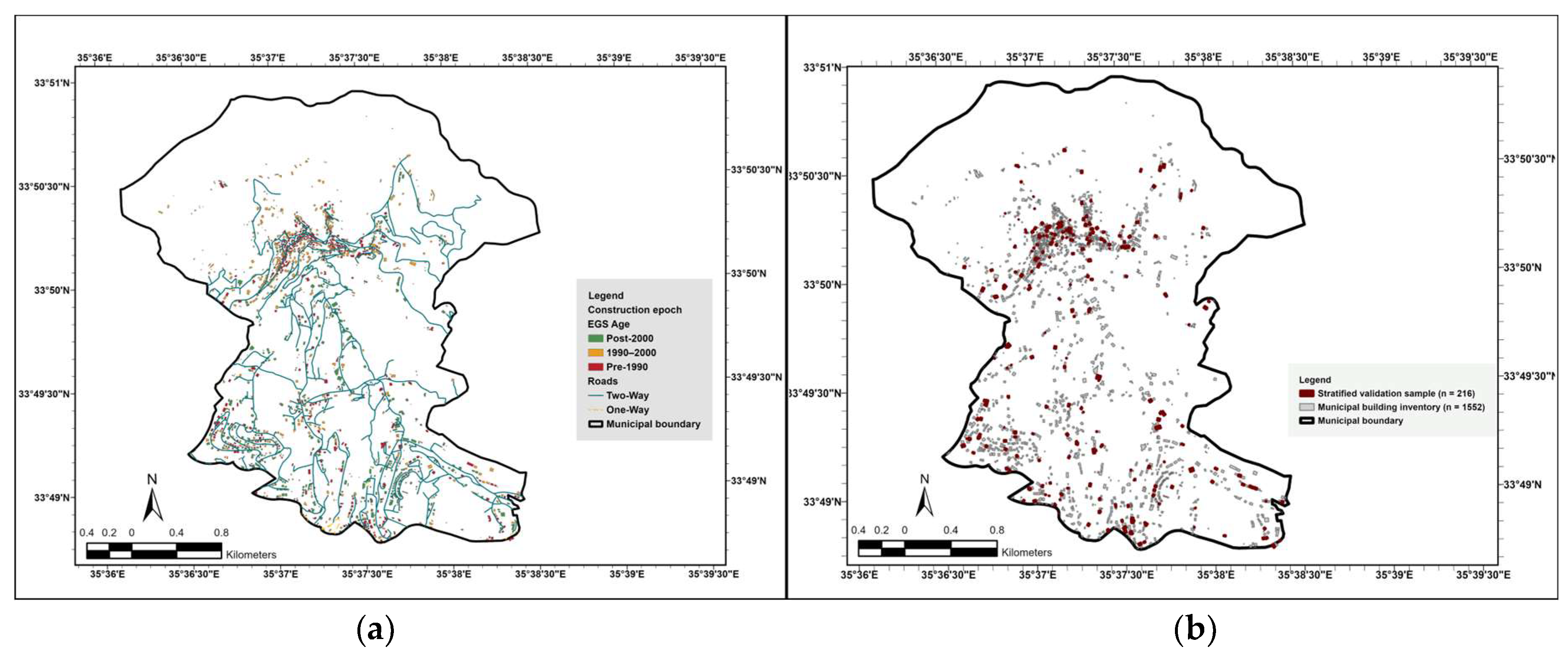
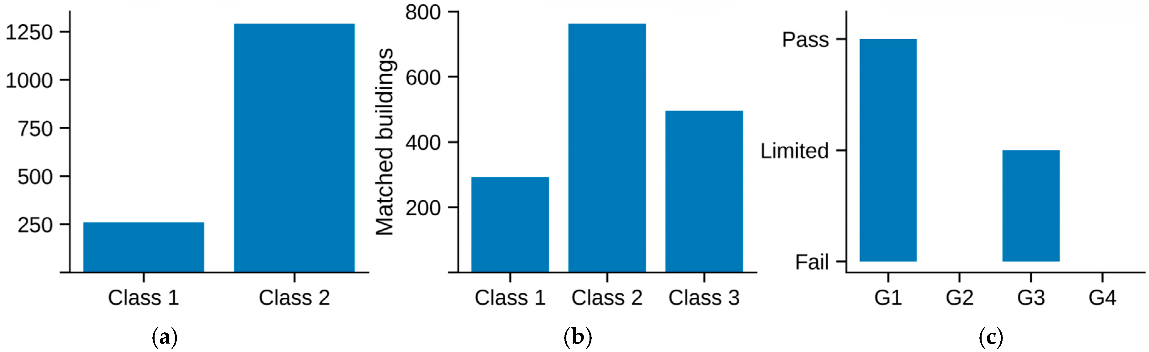
The construction-epoch proxy was derived from the GAIA Version 2024 annual Landsat-based product, which spans 1985–2024 [30,31]. The historical rule used the 1985, 1990, and 2000 annual layers to identify when each pixel first appeared as impervious. Pixels already impervious in 1985 or first detected by 1990 were coded as pre-1990. Pixels first detected between 1990 and 2000 were coded as 1990–2000, and later conversions as post-2000. Each building received the modal raster class within its footprint, with ties resolved by the earliest epoch. The retained scheme assigns ordinal values in order of increasing screening priority: post-2000 (class 1), 1990–2000 (class 2), and pre-1990 (class 3). Applied to all 1552 municipal footprints, the rule assigned 455 buildings to class 1, 697 to class 2, and 400 to class 3 (Figure 3a). Validation used a stratified probability sample of 216 buildings, 72 from each proxy class (Figure 3b).
The epoch boundaries derive from the annual GAIA layers available in the project workflow, not from regulatory milestones. Their alignment with Lebanese code history is what makes the classes interpretable for screening. Pre-1990 buildings predate any national anti-seismic design specification, a period when unreinforced masonry and non-seismically detailed reinforced concrete were prevailing in practice. The 1990–2000 cohort spans Lebanon’s first such specifications (Decree 11266 of 1997) under uneven voluntary uptake. Post-2000 construction is increasingly likely to follow those specifications, which were made mandatory by Decree 14293 of 2005 and strengthened by Decree 7964 of 2012 [75,76,77]. A building’s cohort shows which code applied when it was built, not whether the code was followed.
The proxy estimates the period in which impervious development was first detected in a 30 m pixel. It does not observe construction completion, structural system, material strength, reinforcement detailing, retrofit history, maintenance, occupancy, irregularity, code compliance, or present condition.
The analysis is tied to the named GAIA Version 2024 product, its documented 1985–2024 temporal coverage, and the recovered epoch, masking, and modal-class transfer rules [31]. The original Earth Engine task identifiers, backend execution record, and exact historical cloud-access date were not retained. Two levels of reproducibility are distinguished. Product- and rule-level reproducibility mean that another analyst can obtain the specified product version and repeat the declared classification and transfer logic. Bitwise replication is a stronger claim: an identical value and mask in every exported cell, which normally depends on the exact task, software and backend state, projection request, pyramiding and resampling behavior, export geometry, numeric precision, and file-writing options.
GAIA is one of several global products that records when a surface first became impervious in the Landsat archive; Global 30 m Impervious-Surface Dynamic dataset (GISD30) offers similar 30 m coverage for 1985–2020 [78]. This study audits GAIA because it is the product already in the project archive, not because it is the best available option.

Validation Design and Statistical Assessment

Validation was required because the GAIA-derived epoch is a remote-sensing proxy for the first detected impervious development, not a direct observation of building construction. The analysis therefore asked whether the proxy retained sufficient local discrimination for one narrow, low-consequence municipal triage, and quantified the remaining sampling uncertainty. Chronological plausibility or visual agreement were not treated as evidence of local accuracy. For the low-consequence construction-epoch inspection queue, the case-specific conditional-admission rule required at least 20 classifiable local cases, observations from both binary classes, a point accuracy of at least 0.75, and a bootstrap 95% lower bound of at least 0.60. These thresholds are governance choices for this study, not universal accuracy standards, and they do not authorize damage prediction or fusion with rejected layers.
Reference labels came from a stratified random sample of the 1552 building footprints. The three GAIA-derived epoch classes formed the strata, containing 455, 697, and 400 buildings. Seventy-two buildings were drawn from each, giving a total of 216. Equal allocation supports class-specific accuracy assessments [79]. Municipality-level estimates were post-stratified using the known class proportions. Every building in the inventory therefore had a known inclusion probability. A sampled building stands for 6.3 buildings in the post-2000 stratum, 9.7 in the 1990–2000 stratum, and 5.6 in the pre-1990 stratum. Sample results carry to the municipality by those weights, and not by an assumption about the sample. The design is reported in Supplementary Table S3a and the sample distribution in Figure 3b.
Two interpreters independently reviewed 216 buildings using historical imagery from 1985, 2001, and 2004. The GAIA-derived classes were withheld during interpretation. Presence in 1985 identified pre-1990 buildings, while absence in 2001 followed by presence in 2004 identified post-2000 buildings. Buildings absent in 1985 but present in 2001 could not be assigned to the intermediate 1990–2000 class from imagery alone. Interpreter observations are provided in Supplementary Table S3b.
Buildings unresolved from imagery were checked in the field using reported construction periods, approximate construction years, and available dated documents. Analyses were conducted for the full reference set and for subsets defined by evidence quality. Respondent characteristics are summarized in Supplementary Table S3f.
Following recommended accuracy-assessment and design-based inference practice [79,80], class-specific accuracy and the error matrix were treated as the primary measures. Metrics included user’s and producer’s accuracy, Cohen’s kappa, macro-F1, and F1 for the pre-1990 class, with percentile-bootstrap 95% confidence intervals from 5000 resamples. Gwet’s AC1 is reported alongside kappa because kappa is sensitive to class prevalence [81]. Inter-rater agreement was assessed for the image observations, the classifiability decision, and the adjudicated classes. Agreement on the image observations is primary, because those were obtained independently. Agreement on the adjudicated classes is secondary, because field evidence was collected once per building and shared.

2.6. Gated Layers 2 and 3: Building-Level and Source-Side Soil Products

Two soil layers were generated in the project file along with their production documentation. Both derive from the same CNRS polygons and differ in decision unit, not in source data. The building-level criterion transfers the classification to individual footprints, whereas the source-side field retains it on the 10 m raster grid.
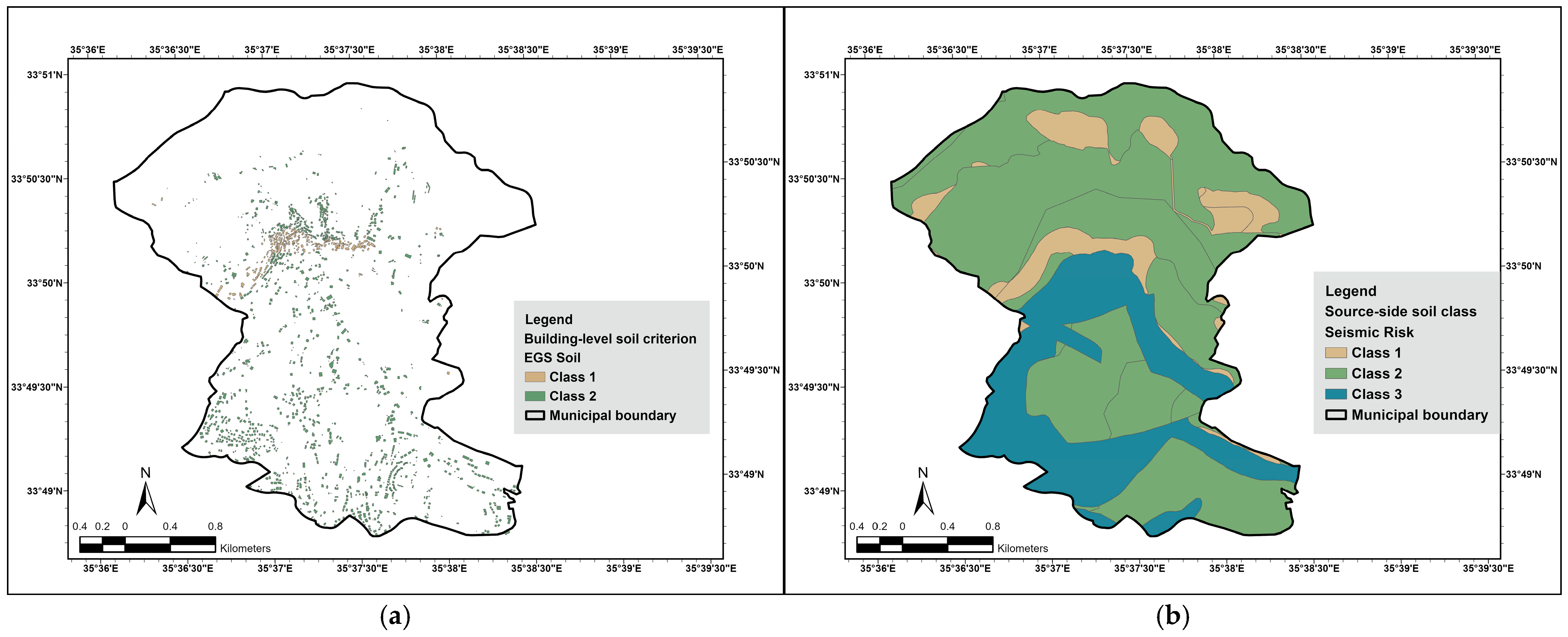
For the building-level soil screening criterion (S in Equation (2)), the CNRS soil polygons were assigned a two-class score. Anthrosols, Cambisols, and Luvisols were assigned class 1; Arenosols, Leptosols, Regosols, and Gleysols were assigned class 2, in order of increasing assigned soil-based screening score. The polygons were then rasterized at 10 m using the filled DEM as the snap raster, and the modal footprint value was transferred to each building (Figure 4a).
These seven reference soil groups, defined in the World Reference Base for Soil Resources [82], describe pedogenesis, not engineering behavior. Anthrosols are soils substantially modified by long-term human activity. Cambisols show only initial horizon differentiation and limited profile development. Luvisols are characterized by clay accumulation in the subsoil. Arenosols are dominated by sandy material with little profile development. Leptosols are shallow soils over hard rock or with abundant coarse fragments. Regosols are weakly developed soils in unconsolidated material. Gleysols form under prolonged water saturation and reducing conditions.
For the source-side soil processing chain (Ss in Equation (3)), the historical lookup grouped Anthrosols, Cambisols, and Luvisols as seismic-risk class 1, Arenosols, Leptosols, and Regosols as class 2, and Gleysols as class 3, in order of increasing assigned soil-based screening score (Figure 4b). This three-class field was rasterized to the common grid and supplied the soil term of the project ERI and related raster-hazard calculations.
The two products therefore express the same grouping at different decision units. The building criterion separates only the most favorable source class from all others, so source-side class 3 is folded into building class 2. The archive documents both schemes but records no rationale for that reduction. The gate question is whether pedological classes can carry seismic screening priority at the building level without local site-response evidence.
For the Newmark processing chain, two soil products were used. Details are provided in Supplementary Text S2.

2.7. Gated Layer 4: Exploratory Age-Soil Index

The building-level ASI (Figure S4) was constructed as
ASIi = 0.625 Ai + 0.375 Si,
where ASIi is the dimensionless index for building i, Ai is the ordinal construction-epoch class, and Si is the ordinal two-class soil score. Initially, the project’s ASI was generated with three-factor weighting. Supplementary Text S3 provides details on ASIi. The retained project breaks, 1.667 (5/3) and 2.333 (7/3), divide the nominal 1–3 ordinal rating scale into three equal-width bands: ASIi < 1.667 was Low, 1.667 ≤ ASIi < 2.333 was Moderate, and ASIi ≥ 2.333 was High. The breaks were fixed before the sensitivity audit and were not fitted to sample quantiles or observed class frequencies.
The counterfactual sensitivity test varied the age weight across 0.50, 0.55, 0.60, 0.625, 0.65, 0.70, and 0.75; the soil weight was one minus the age weight. This analysis measured classification response to weights. It did not establish the soil layer’s eligibility. The gate question for this index is whether a weighted combination of ordinal codes remains admissible when one of its inputs is not.

2.8. Gated Layer 5: Newmark Displacement Raster

The pronounced terrain relief and the explicit role of slope in infinite-slope and Newmark calculations motivated the inclusion of a Newmark displacement processing chain among the candidate evidence layers [83,84]. The project implemented a Newmark sliding-block workflow [35,36] on the common 10 m EPSG:32636 grid, calculating and masking a factor-of-safety surface (FS), generating critical acceleration (ac) and Arias intensity (Ia), and thresholding the resulting Newmark displacement using the project’s historical 30 cm cutoff together with two retained post-processing rules (a 5° slope cutoff assigning FS = 10, and NoData masking for FS ≤ 1 or sub-5° cells); the full processing chain, reclassification procedure (Figure S5), and rule rationale are documented in Supplementary Texts S2 and S4, with equations given in Appendix A. The gate question for this processing chain is whether the stored Newmark displacement raster can be reproduced from its documented generator and applied within its calibration domain.

2.8.1. Factor-of-Safety Reconstruction Audit

The reconstruction audit was necessary because the factor of safety is the upstream input to critical acceleration, Newmark displacement, threshold classes, and the ERI. An undocumented error at this stage would propagate through every downstream raster. The stored surface was treated as deterministic only in the limited computational sense that the file contains one fixed value and mask per grid cell and the intended map-algebra equation is deterministic for fixed input. This does not imply that its provenance or parameters are known. The audit tested 240 candidate configurations spanning the documented cohesion, friction-angle, dry-unit-weight, pore-pressure, equation, and slab-thickness alternatives. A valid deterministic reconstruction required a matching grid and mask plus near-numerical identity, not correlation alone. The retained constant-depth configuration was the one minimizing RMSE and MAE, not the one maximizing correlation. Its parameters are given in Supplementary Table S5.
Each diagnostic addressed a different failure mode. The Pearson correlation coefficient measured spatial pattern similarity, not equality. Root mean square error (RMSE), mean absolute error (MAE), bias, maximum error, and relative-error percentiles quantified magnitude agreement. Mask comparison confirmed that the same cells were evaluated in both surfaces. The algebraic inversion of Appendix A, Equation (A1) tested whether the slab thickness implied by the stored values remained positive and close to its stated value.

2.8.2. Calibration-Domain and Signal-Validity Analysis

This analysis was required because the reproducible code can still produce values outside the range over which its empirical relation was calibrated. G2 therefore tested whether each cell satisfied the stated applicability interval 0.02 ≤ ac ≤ 0.40 g. G3 tested whether each operational displacement threshold contained values produced within the calibration interval. The gates were evaluated independently so that passing one could not conceal failure of another. Non-flat cells were classified as statically unstable (FS ≤ 1, equivalently ac = 0 under Appendix A, Equation (A2)), below domain (0 < ac < 0.02 g), within domain (0.02 ≤ ac ≤ 0.40 g), or above domain (ac > 0.40 g) (Figure S6). Flat placeholders were kept as a separate category. At the building level, ArcGIS Tabulate Area measured footprint area within each domain class; ordinal codes were not averaged. A building was entirely in domain when all evaluable non-flat area was in domain, partly in domain when both in-domain and other evaluable areas were present, and without in-domain area when none of its evaluable area fell inside the interval.
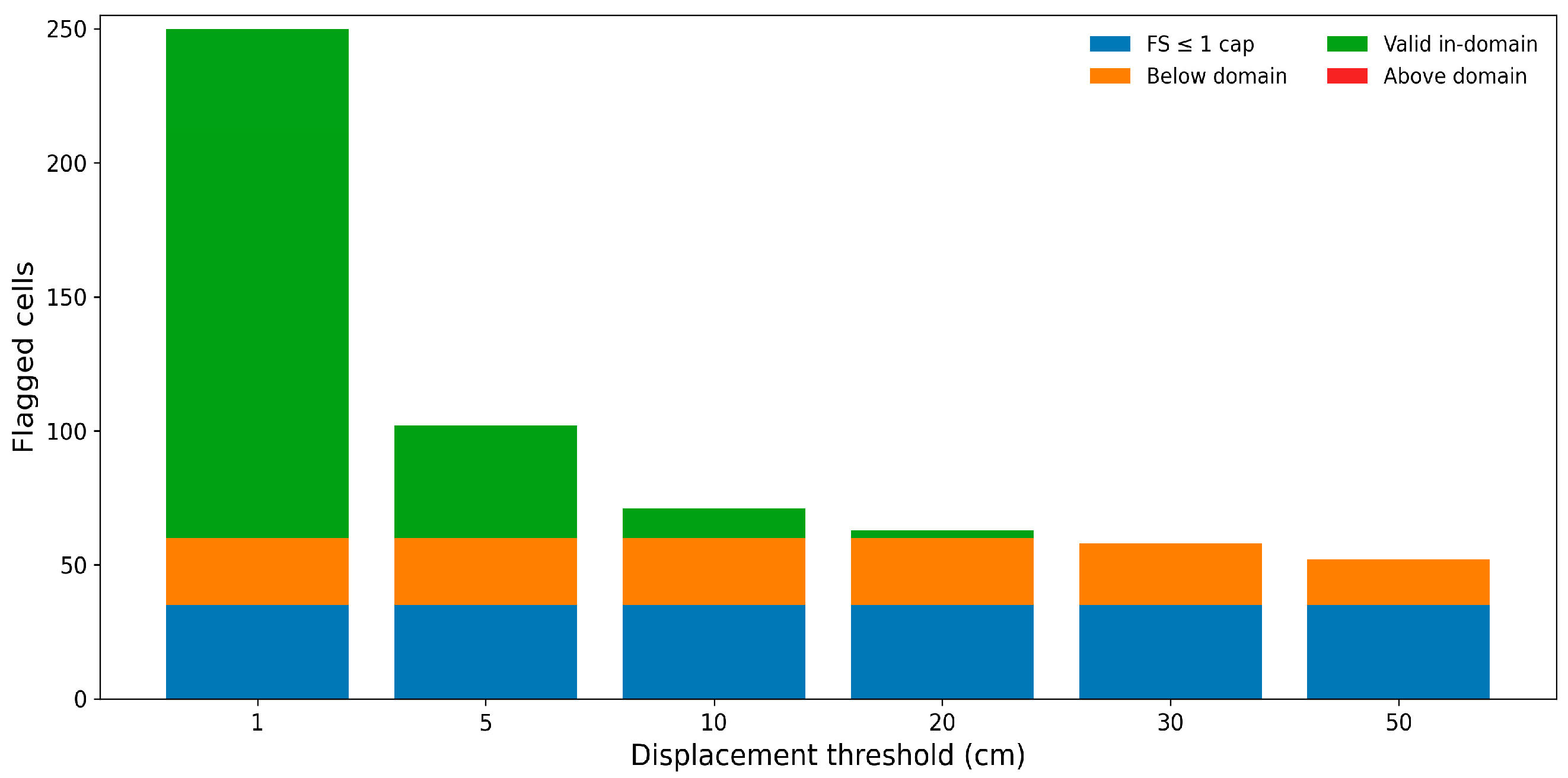
For G3, displacement thresholds of 1, 5, 10, 20, 30, and 50 cm were tabulated by static stability and calibration-domain status. Each category was counted separately: cap assignments, below-domain extrapolations, valid in-domain predictions, and above-domain cells. The 30 cm cutoff was inherited from the historical project classification as the boundary of its High displacement class. It was not estimated from the Aabadiyeh observations. The audit retained 30 cm to evaluate the exact historical decision, while the six-threshold series tested whether the signal-validity conclusion depended on that choice.

2.9. Gated Layer 6: Earthquake Risk Index

The historical ERI processing chain first aligned the stored Newmark-displacement, peak-ground-acceleration, slope-risk, and source-side soil-class rasters to the common 10 m grid and applied the project reclassification lookups. ArcGIS Weighted Sum then combined the ordinal inputs with fixed coefficients of 0.40, 0.25, 0.20, and 0.15, respectively; the resulting values were assigned to the project’s five ERI classes.
The ERI (Figure S7) was reconstructed as
ERI = 0.40 N + 0.25 P + 0.20 T + 0.15 Ss,
where N is the reclassified Newmark displacement (3 classes), P is reclassified peak ground acceleration (3 classes), T is slope-risk class (1–2), and Ss is the source-side three-class soil value (3 classes).
The ERI was classified in an ordinal manner and assigned five classes (Very Low/Low/Moderate/High/Very High). Supplementary Text S5 provides details on ERI construction.
Three reproducibility levels were distinguished. Formula-level reproduction means that stored component rasters can be recombined with Equation (3). Component-level reconstruction means that each component can be reproduced from its original inputs and documented operations. Archived-workflow reconstruction requires the full sequence of grid, resampling, masks, reclassification, component generation, and export to be recovered. These levels were reported separately because a correct weighted sum says nothing about where its components came from. The gate question for this composite is whether a reproducible formula is enough to admit a composite when its component inputs fail their own gates.
Supplementary Table S11 summarizes the class codes assigned to each candidate, together with the scale on which each is expressed. It makes one property explicit across all candidates. Every code is an ordinal rank, so the spacing between successive classes is not calibrated and the codes carry no interval or ratio meaning. This matters for the composite, because Equation (3) combines these ordinal codes as if the steps between them were equal.

2.10. Raster-to-Building Transfer Audit

The transfer audit was required because the decision unit was the building footprint, while the Newmark and ERI evidence was stored on a 10 m raster. Even a valid cell-level model can yield a biased municipal queue if small polygons, narrow polygons, mask-edge buildings, or buildings without a cell center are silently omitted. Transfer completeness was defined as the number of decision units receiving a valid transfer record divided by the number of target decision units. Missing transfer records were treated as missing evidence, not as zero-risk, low-priority, or NoData-free observations.
Historical transfer used ArcGIS Tabulate Area with the building source identifier (SRC_OID) as the zone field and the project critical-acceleration domain raster as the class raster. The resulting class-area fields were joined back to the complete 1552-building inventory. An anti-join identified footprints with no tabulation record, after which footprint area, perimeter, compactness, one-cell area fraction, representative class, and representative-point validity were recorded. Area tabulation was chosen because a categorical class carries no meaningful average; classes were summarized by the share of footprint area in each class. The 100 m2 split corresponds to one 10 m × 10 m cell and was used diagnostically to separate sub-cell scale effects from omissions that size alone does not explain.

2.11. Uncertainty and Sensitivity Analysis

This audit was performed to determine whether the admission decisions depended on sampling variation, discretionary weights, model alternatives, thresholds, or raster–vector transfer. Bootstrap intervals quantify uncertainty in the construction-proxy validation estimates. The age-weight scenarios measure whether the ASI classes change as the age weight varies. The 240-configuration family examines model and provenance uncertainty. Threshold tables examine whether the G3 outcome depends on the threshold chosen, and the omission ledger measures transfer completeness.
The admission rule was deliberately not replaced by a robustness score. Stable output under weight variation could not admit a layer that failed applicability or input support. Conversely, a conditionally admitted proxy could be retained for low-consequence triage even though its interval estimates remained wide, provided its limitations were explicit.

3. Results

3.1. Construction-Epoch Distribution, Validation, and Gate Decision

The three-class chronology assigned 455 buildings to post-2000, 697 to 1990–2000, and 400 to pre-1990 (Table 4). The counts sum to the complete inventory of 1552 buildings.
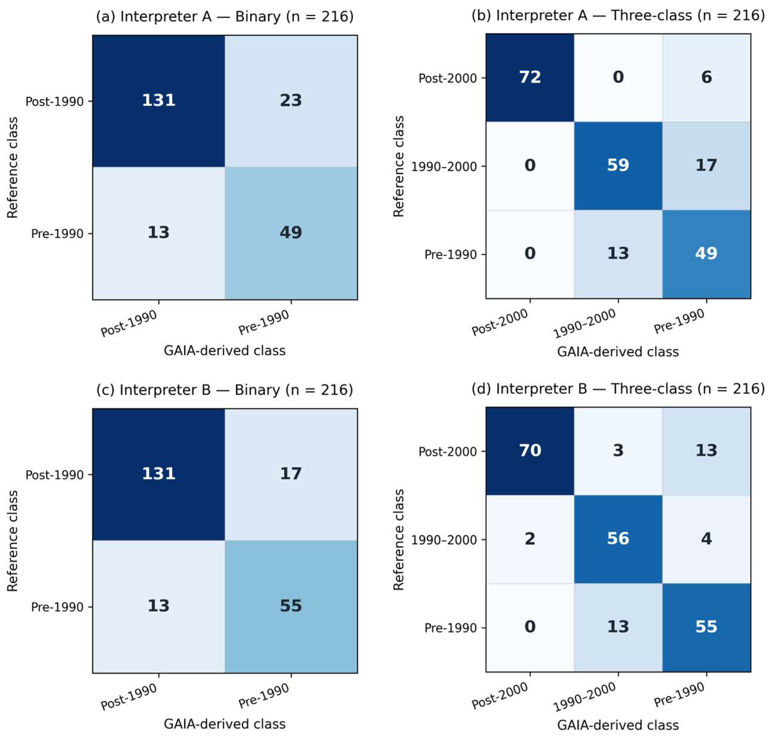
Both interpreters classified all 216 sampled footprints (Figure 5). Among the 59 footprints classifiable from imagery alone by both interpreters, three-class agreement was 0.915 (κ = 0.832, 95% confidence interval (CI) 0.670–0.965). Agreement on image-based classifiability across all 216 footprints was κ = 0.720 (0.618–0.812). For the adjudicated classes, three-class agreement was 0.838 (κ = 0.756, 0.681–0.829), and binary agreement was 0.870 (κ = 0.692, 0.581–0.795) (Supplementary Table S3c). Complete confusion matrices and validation metrics are provided in Supplementary Table S2.
Against the two independent reference sets, binary accuracy for the pre-1990 class was 0.833 (0.782–0.880) and 0.861 (0.815–0.907), with κ = 0.612 (0.494–0.724) and 0.683 (0.570–0.782), respectively. Pre-1990 F1 scores were 0.731 and 0.786, and three-class accuracy was 0.833 and 0.838. Both binary results satisfied the rule defined in Section Validation Design and Statistical Assessment. Accuracy remained similar for footprints resolved from imagery alone (0.779, 0.667–0.862; n = 68), those supported by documentary evidence (0.793, 0.700–0.864; n = 92), and after excluding low-confidence respondent recall (0.825, 0.753–0.879; n = 137) (Supplementary Table S3e).
After post-stratification to the municipal class distribution, the estimated numbers of pre-1990 buildings were 398 (322–474) and 431 (358–505), compared with 400 assigned by the proxy. Population-weighted binary accuracy was 0.837 (0.788–0.886) and 0.858 (0.811–0.906). User accuracy for the pre-1990 class was 0.681 (0.566–0.777) and 0.764 (0.654–0.847), and producer accuracy was 0.684 and 0.708. Of the 400 buildings assigned to the inspection queue, an estimated 272–306 were pre-1990, while approximately 126 pre-1990 buildings were outside the queue (Supplementary Table S3d). These are municipality-level estimates. They apply to the 1552 buildings together, and they assign no status to an individual building.
G1 passed at the product- and rule-level standards defined in Section 2.5: the 1985, 1990, and 2000 annual layers, class rules, and modal-class building transfer reproduced the reported feature totals. Bitwise identity with the original cloud export was not claimed for this candidate. G2 received a conditional pass for low-consequence municipal triage, but not for structural prediction. G3 passed because the decision-relevant pre-1990 class was occupied and separable, and the binary split retained discriminatory information. All three cohorts were populated, but the intermediate cohort was not used as a decision class. G4 received a conditional pass. The binary results satisfied the declared rule for both independent reference sets and remained above the threshold across all evidence-quality subsets. Reference labels also showed good reproducibility between interpreters. The pass remained conditional because the intermediate class could not be resolved from the available imagery, some reference labels relied on respondent recollection, and user’s and producer’s accuracy for the decision-relevant class were lower than the overall agreement.
The proxy was therefore conditionally admitted as a standalone method for forming a preliminary pre-1990 inspection queue. No structural meaning beyond construction-epoch screening was assigned.

3.2. Building-Level and Source-Side Soil Products Evidence and Gate Decision

The two-class building rule reproduced the stored counts of 260 class-1 buildings and 1292 class-2 buildings. The source-side product matched 1550 footprints: 292 in class 1, 763 in class 2, and 495 in class 3; two footprints did not match a source polygon (Table 5, Figure 6a,b). These products were computationally distinct and were not merged during the audit. The building product is a two-class reduction in the source-side scheme. Source classes 2 and 3 are folded into building class 2, while 260 of the 292 source-class-1 footprints retain building class 1. The 32 exceptions follow from the transfer rule rather than from the classification. The building value is the modal 10 m cell within each footprint, not the class of the polygon the footprint matches, so a footprint spanning a class boundary can take the neighboring class. The same soil code therefore appears under both building classes in the lookup table. The complete source-to-building soil lookup table, including the 32 source-class-1 footprints assigned to building class 2 and the two unmatched footprints, is reported in Supplementary Table S4.
The two-class rule passed G1 and failed G2: it assigned seismic screening priority at the building level from pedological classes, with no locally validated site-response evidence. G3 was Limited: class 2 contained 83.25% of the inventory, so the criterion separated few buildings from the rest. G4 failed because no local VS30 measurements, boreholes, engineering site classes, laboratory tests, or observed amplification supported the assigned seismic meaning. These four outcomes are summarized in Figure 6c. G1 for the source-side field was recorded as partial provenance and not as a pass. The three-class lookup and its rasterization to the common grid are documented and the class counts reproduce across the 1550 matched footprints. The archive records neither how the polygon-matching step treated the two unmatched footprints nor any rationale for the subsequent reduction from three classes to two. The source-side field had the same applicability and support limitations. Both soil products were rejected for operational building prioritization.

3.3. Exploratory ASI Counterfactual and Gate Decision

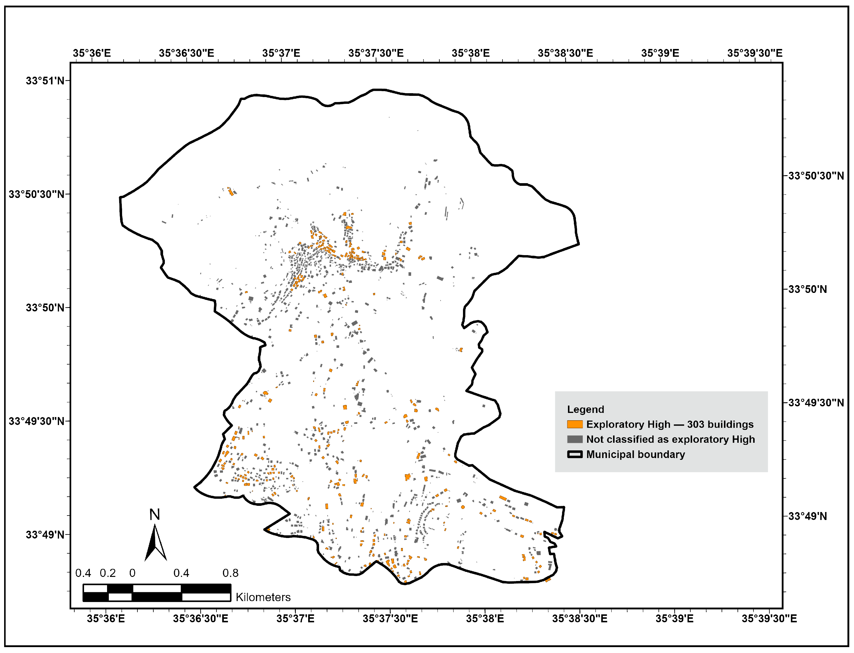
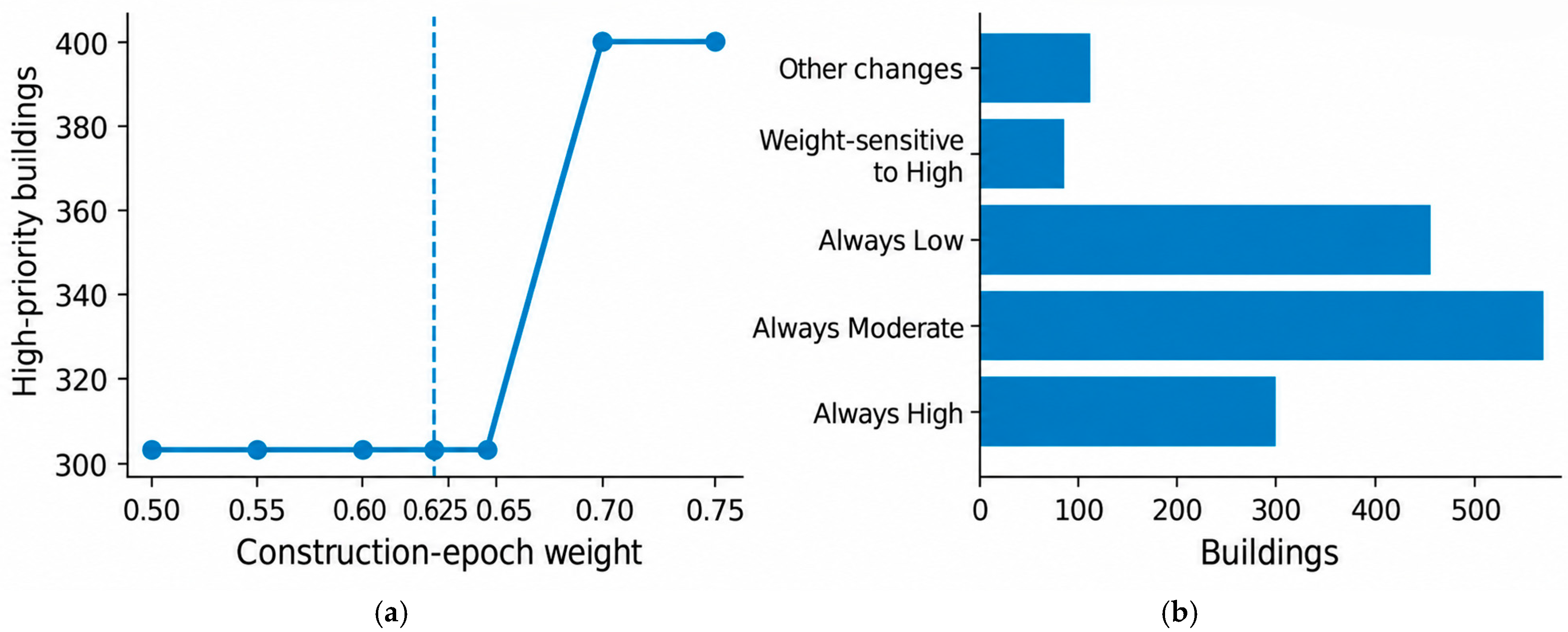
The historical ASI equation reproduced 584 Low, 665 Moderate, and 303 High buildings. Figure 7 shows the spatial distribution of the 303 buildings classified as exploratory High by the ASI. The High count remained at 303 for age weights from 0.50 through 0.65 and increased to 400 at 0.70 and 0.75 (Table 6, Figure 8a). Across all scenarios, 1326 buildings (85.44%) never changed class, whereas 226 (14.56%) changed at least once (Figure 8b). The 97-building increase in the High count is not the same quantity as the 226 buildings that changed class across any scenario.
The composite passed G1 at formula level and passed G3 with three occupied classes, but it inherited the soil layer’s G2 and G4 failures. It was retained as Exploratory only and did not enter the final municipal screen. The Figure 7 map is therefore retained as a counterfactual diagnostic showing where the historical fusion concentrated priority, not as an operational priority surface.

3.4. Newmark Evidence and Gate Decisions

3.4.1. Factor-of-Safety Reconstruction Results

Both documented post-processing operations reproduced exactly one assigned FS = 10 where slope was below 5°, and the other converted cells with FS ≤ 1 or slope below 5° were assigned to NoData. This establishes that the historical cleaning and stable-slope mask rules were recovered. It does not reconstruct the raw factor-of-safety generator, because those operations act on whatever raw values they receive and carry no information about which c, φ, γd, ru, z, or equation variant produced them.
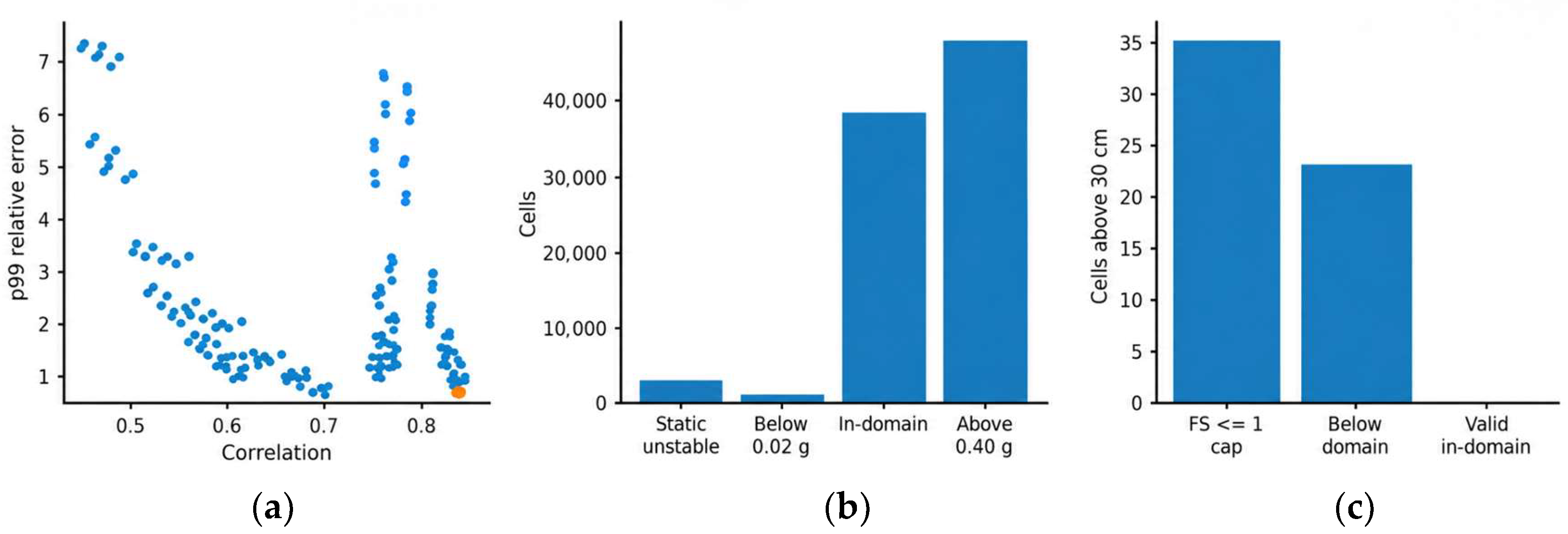
Among the 240 tested configurations, the minimum-RMSE/minimum-MAE constant-depth configuration yielded r = 0.840, RMSE = 1.345, MAE = 1.184, and a 99th-percentile relative error of 0.809 (Figure 9a). Correlation was not used as the selection criterion: the retained configuration ranked first of 240 on both RMSE and MAE but only sixth on correlation, and every configuration with a higher correlation performed worse on absolute error. Algebraic inversion across 87,490 evaluable cells produced 22,409 non-positive implied depths (25.61%). The corrected common mask used for this reconstruction contained two fewer valid cells than the project raster mask tabulated in Section 3.4.2 (87,492). The implied-depth coefficient of variation was 22.239, and 2717 cells (3.105%) were within ±1% of the 2.4 m test depth. The observed systematic magnitude, tail, and inversion failures contradict generation by every tested member. This conclusion concerns the stored raster-to-candidate link; it does not indicate that Appendix A, Equation (A1) is physically invalid.
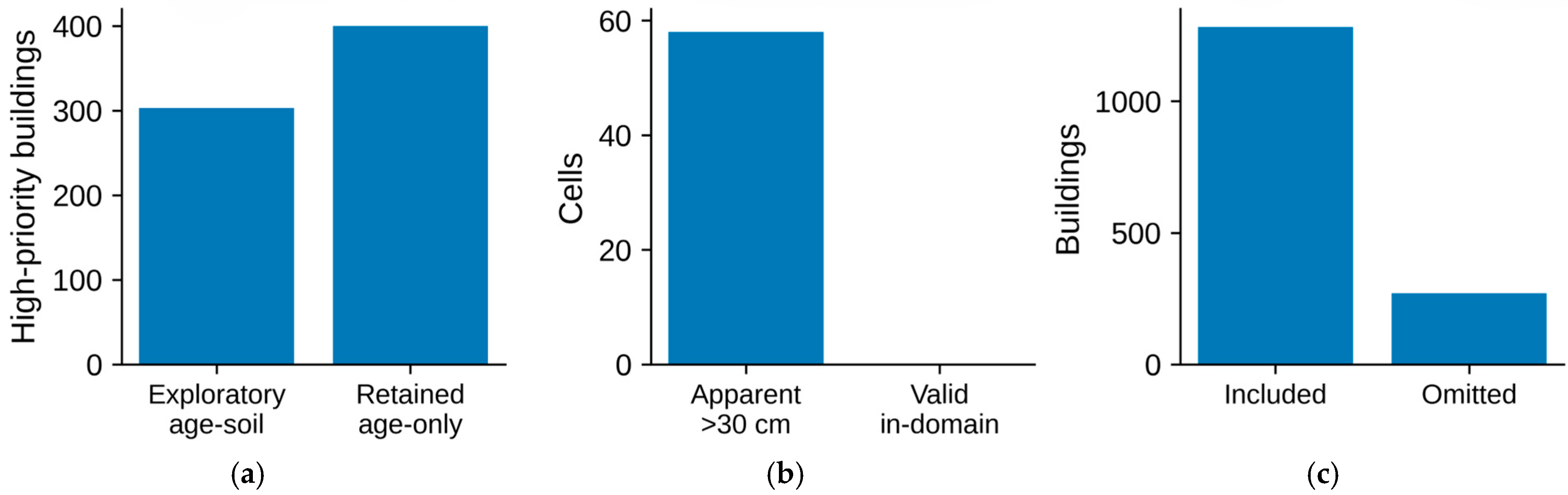
The remaining panels report the two downstream diagnostics that depend on this reconstruction. Figure 9b classifies the 87,492 non-flat project cells by critical-acceleration applicability: 2012 are statically unstable, 545 fall below 0.02 g, 38,230 lie within the stated 0.02–0.40 g domain, and 46,705 exceed 0.40 g. Figure 9c gives the composition of the project 30 cm displacement class as 35 FS ≤ 1 cap values and 23 below-domain extrapolations, with no valid in-domain cells. Both are taken up in Section 3.4.2 and Section 3.4.3 respectively.
Configuration-level results for all 240 tested combinations, including the parameters of the retained configuration, are reported in Supplementary Table S5; the original row-level export was not retained in the project archive. The post-processing comparisons and valid-mask results are in Supplementary Table S6.
G1 therefore failed at the component and raw-generator levels. The preserved cleaning rules passed as post-processing steps, but they carry no information about how the underlying surface was produced.

3.4.2. Critical-Acceleration Applicability

The domain audit separated 2654 flat-placeholder cells from 87,492 non-flat cells. Among the non-flat cells, 2012 were statically unstable, 545 were below 0.02 g, 38,230 were within 0.02 ≤ ac ≤ 0.40 g, and 46,705 exceeded 0.40 g. The outside-domain total was therefore 49,262 cells, or 56.30% of non-flat cells.
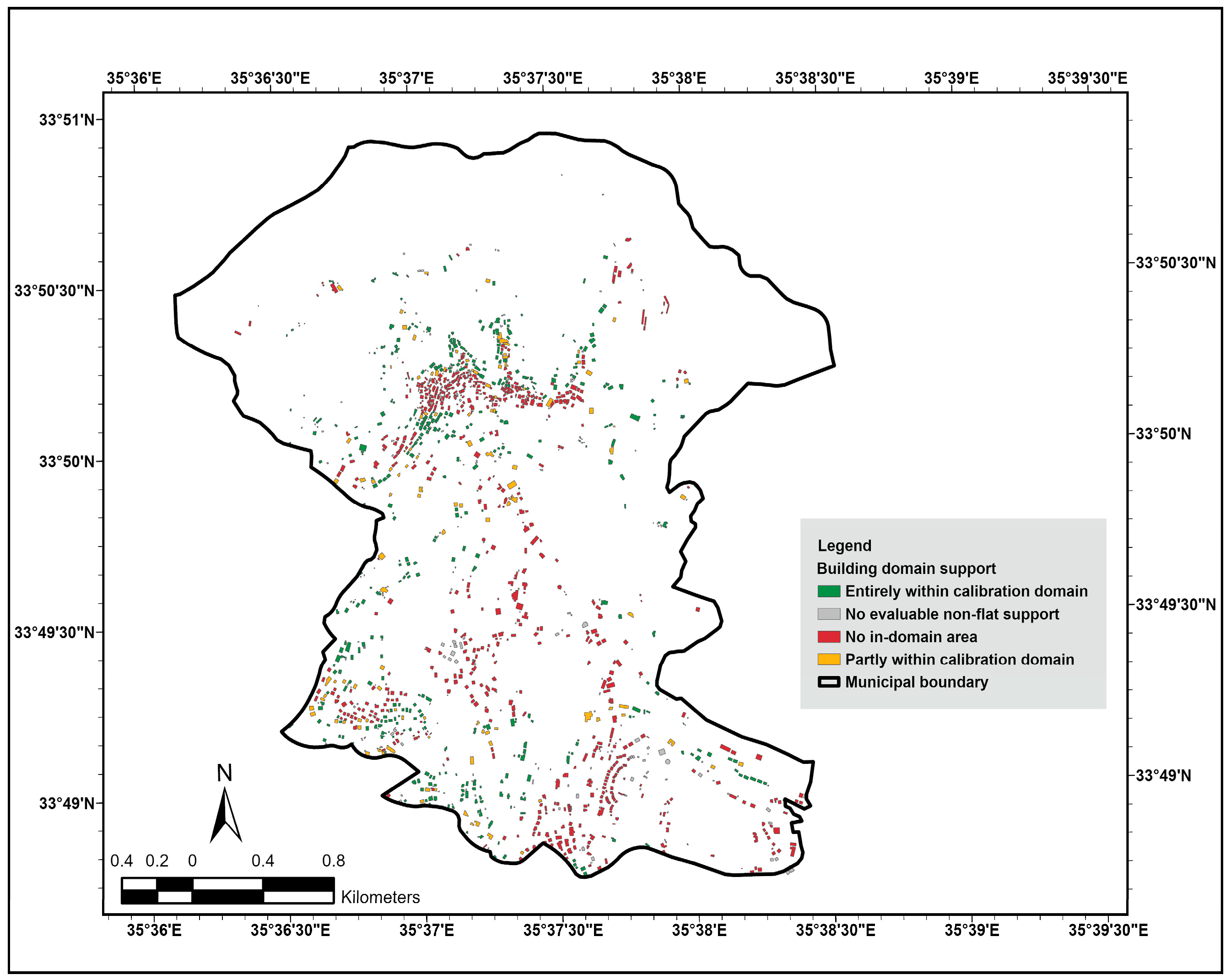
At the building level, 1243 footprints contained an evaluable non-flat area. Of these, 458 were entirely in domain, 111 were partly in domain, and 674 had no in-domain area. Table 7 reports percentages against the correct evaluable-building denominator.
G2 failed for the project implementation: 56.30% of non-flat raster cells lay outside the stated critical-acceleration interval, predominantly above it, and only 458 buildings were fully supported by in-domain values (Figure S8).

3.4.3. Newmark Signal Validity and Admission

At the project’s 30 cm threshold, 58 cells were flagged. Thirty-five were imposed cap values for FS ≤ 1, and 23 were below-domain extrapolations. None was a valid in-domain prediction. Valid in-domain cells occurred at lower thresholds: 190 at 1 cm, 42 at 5 cm, 11 at 10 cm, and 3 at 20 cm (Figure 10). G3 was therefore threshold-dependent and failed for the 30 cm decision class. The full calibration-domain and threshold tabulations are reported in Supplementary Table S7.
G4 also failed. None of the strength, pore-pressure, or geometry inputs rested on local observation. Cohesion, friction angle, and dry unit weight were regional literature proxies transferred through pedological classes. Pore-pressure conditions were represented by a topographic wetness index, not measured groundwater. Slab thickness was assigned a single constant value of 2.4 m. The site term was taken from a VS30 mosaic product, not from local measurement. Input support was therefore insufficient for a building-level displacement claim, independently of the provenance and calibration-domain failures. The Newmark displacement raster was rejected because G1, G2, and G4 failed independently of threshold choice. The result concerns the project implementation evaluated here, not the Newmark method in general.

3.5. ERI Reproducibility, Admission, and Gated Decision

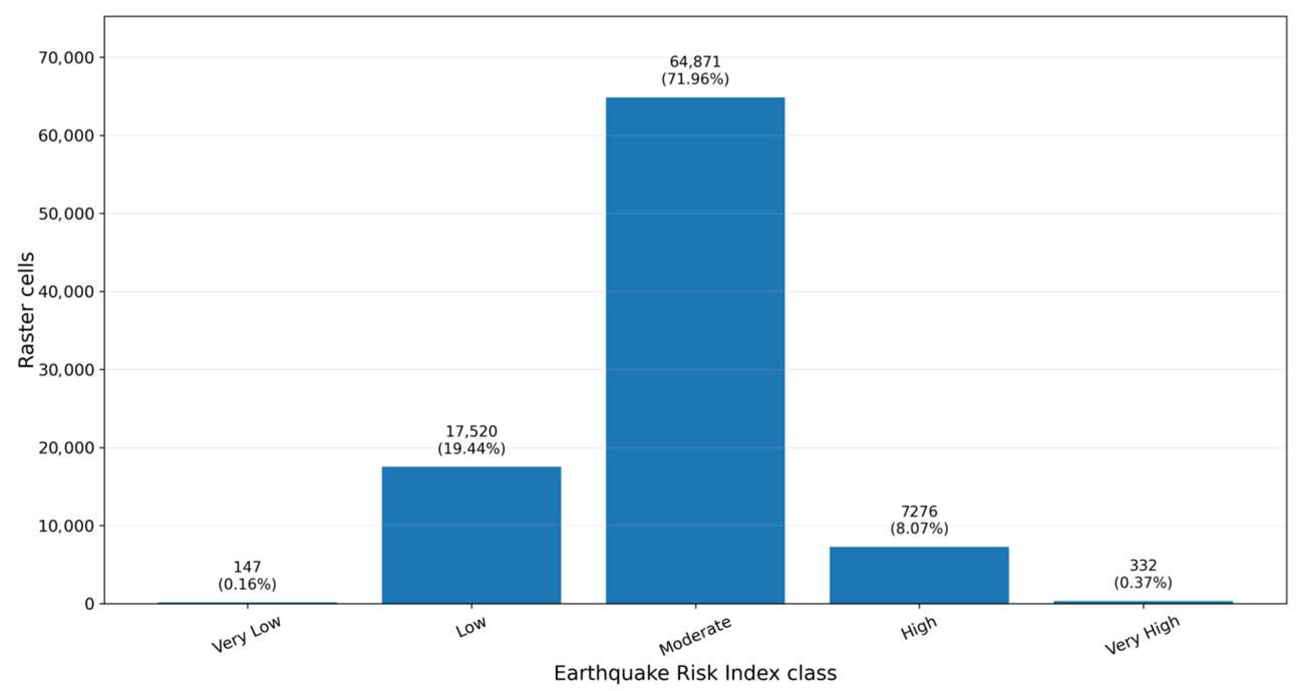
Equation (3) reproduced a five-class ERI over 90,146 cells. The mean class value was 2.890 with standard deviation of 0.533. Very Low covered 147 cells (0.16%), Low 17,520 (19.44%), Moderate 64,871 (71.96%), High 7276 (8.07%), and Very High 332 (0.37%) (Figure 11). This was a formula-level pass using stored component rasters. Two of the four Equation (3) inputs also carried limited discriminatory range. The shaking component’s class boundaries were separated by 0.013 g, and the slope-risk component was binary by construction. Together these account for 0.45 of the declared weight, which is consistent with the concentration of 71.96% of cells in the single Moderate class. G3 was therefore recorded as numerical variation present but not sufficient. All five classes were occupied, but that occupancy reflects arithmetic spread, not discrimination. This is because most of the municipality resolves to a single class and nearly half the declared weight comes from inputs with almost no range.
Component-level provenance failed because the stored Newmark factor-of-safety input could not be traced to a recorded execution. The intended equation, slab thickness, common grid, and post-processing rules are now documented, so it is no longer accurate to say that the factor-of-safety method or grid geometry is wholly unknown. However, full archived-raster reconstruction still cannot be claimed because the exact historical input versions, per-component resampling and reclassification history, raw-raster execution record, masks, export settings, and intermediate checksums are incomplete. G1 is therefore recorded as a Formula pass; component/input-chain failure. G2 and G4 failed through the Newmark and soil inputs, and the ERI was rejected for municipal building prioritization.
A verified validity-mask map could not be reconstructed independently of the inherited Newmark and soil limitations. Figure 11 therefore reports the class distribution only, and the project raster is retained as an audit product rather than an operational risk surface.

3.6. Raster-to-Building Transfer Completeness

The zonal tabulation omitted 270 of 1552 footprints, corresponding to 17.40% of the inventory and a transfer completeness of 82.60%. Of the omitted footprints, 245 (90.74% of omissions) were smaller than 100 m2 and 25 (9.26%) were at least 100 m2. Omitted areas ranged from 0.65 to 726.56 m2, with median 39.47 m2 and mean 52.60 m2. Small-footprint concentration indicated a scale effect. Among the 25 larger omissions, 11 had no valid representative-point class, including the five largest footprints indicating absent raster support. The remaining 14 had valid representative-point classes and therefore implicate grid alignment or the tabulation rule rather than missing data. Figure 12 shows the raster-to-building transfer and building-domain accounting.
The complete omission ledger and summary diagnostics are reported in Supplementary Table S8; missing transfer records were preserved as missing evidence and were never interpreted as low or absent risk.

3.7. Systematic Testing of Omitted Footprints

Omitted and retained footprints were compared by morphology, spatial distribution, and construction-epoch class (Supplementary Table S8a–d). Re-execution of the archived procedure reproduced the omission set exactly (Supplementary Table S8e). Omitted footprints were substantially smaller than retained footprints (median area: 39.45 vs. 225.90 m2; Mann–Whitney U, Benjamini–Hochberg-adjusted p < 10−100; Cliff’s δ = −0.879) and had smaller perimeters (δ = −0.859). Differences in vertex count (δ = −0.253) and compactness (δ = 0.084) were limited. A logistic model including log area, compactness, vertex count, and a quadratic spatial trend achieved an area under the receiver operating characteristic curve (AUC) of 0.945, with log area providing most of the discrimination.
Omitted footprints were spatially clustered under a random-labeling null. On a k = 8 nearest-neighbor graph, the observed omitted–omitted join count was 496, compared with a null mean of 374.8 (pseudo-p = 0.001; 999 permutations). No spatial term was significant in the multivariate model, indicating that the clustering followed the spatial distribution of small buildings, although local spatial structure cannot be excluded.
Omission also differed by construction-epoch class (χ2 = 19.483, degrees of freedom (df) = 2, p = 5.9 × 10⁻⁵), although the association was weak (Cramér’s V = 0.112). Epoch alone showed limited discrimination (AUC = 0.575; McFadden pseudo-R2 = 0.014), compared with AUC = 0.940 and pseudo-R2 = 0.499 for epoch and log footprint area together. Median footprint areas were 152.7 m2 for 1990–2000, 222.8 m2 for pre-1990, and 220.9 m2 for post-2000 buildings. Accordingly, the odds ratio for omission in the 1990–2000 class relative to pre-1990 changed from 1.86 (95% CI: 1.32–2.61) before adjustment to 0.58 (0.35–0.95) after adjustment for area.
The marginal omission rates were 13.3% (95% CI: 10.3–16.9) for pre-1990, 22.1% (19.2–25.3) for 1990–2000, and 13.9% (11.0–17.3) for post-2000 buildings. The pre-1990 class was therefore not preferentially depleted from the inspection queue. After adjustment for footprint size, however, the pre-1990 class was the most likely to be omitted, showing that its lower marginal rate followed from its larger average footprint size.
The omission affected the rejected ERI/ASI chain but not the retained construction-epoch output. If the omitted footprints had received a transfer record, the counterfactual ERI/ASI queue would range from 303 to 573 buildings. The admitted construction-epoch queue remained at 400 because the modal footprint transfer assigned an epoch class to all 1552 buildings.

3.8. Final Gate Matrix

Table 8 consolidates the four-gate outcome for each of the six audited candidates, pairing every gate decision with the operational consequence of admitting or excluding that product.

3.9. Decision Consequences of Admission Before Fusion

The conditionally admitted construction-epoch proxy retained 400 pre-1990 buildings as a preliminary inspection queue. The exploratory ASI overlay had classified 303 buildings as High. Excluding the unsupported soil criterion removed the mechanism by which the soil score had suppressed 97 pre-1990 buildings below the High threshold.
The Newmark audit found no valid in-domain prediction among the 58 cells in the 30 cm class: 35 were caps and 23 were below-domain extrapolations. The transfer audit identified 270 buildings omitted from historical raster tabulation. The ERI formula was recoverable, but its inherited gate failures prevented its operational use. No building-level ASI–Newmark composite was produced because no documented generating rule existed for such a product.
Figure 13 presents these outcomes in the form in which they reach the municipality. Figure 13a contrasts the exploratory High set with the retained age-only queue, Figure 13b decomposes the 30 cm Newmark class by evidential status, and Figure 13c reports the raster-to-building transfer, in which 1282 of the 1552 buildings in the footprint were tabulated and 270 were omitted.

3.10. External Reference-Case Verification

Cases 1 and 2 were assessed by two authors before the case set was extended. Both reached the same outcome at every gate. GAIA was conditionally admitted and SoilGrids rejected. Multi-Attribute Building Dataset of China (CMAB) reports 82% building-level categorical consistency and notes that impervious-surface timing is not always synchronous with construction [62]. International Soil Reference and Information Centre (SRIC) advises against local-scale use, and Poggio et al. report divergence against gridded Soil Survey Geographic database (gSSURGO) [63,64]. Both authors cited these statements. Their records are held separately from the results below.
Two independent assessors then scored all four cases. They agreed on 13 of 16 gates (81.25%). For SoilGrids, G3 was recorded as numerical variation present but not sufficient by one assessor and limited by the other. For the landslide product [65], G3 was threshold-dependent and limited. For INFORM Lebanon [66,67], G4 was fail and conditional pass. Each pair is adjacent in the permitted vocabulary. The two G4 reasons cite the same evidence: the available evaluations assess the global index at national scale and do not test the Lebanon subnational model [68,69]. The assessors differed on whether indirect support is adequate for a low-consequence purpose.
Dispositions agreed on all four cases (100%). GAIA and the landslide product were conditionally admitted. GAIA was conditionally admitted independently by both authors and both external assessors. The external assessors had no access to this study’s own results. SoilGrids and INFORM were rejected. Applying the rules of Section 2.4.1 to each assessor’s own gate outcomes reproduces the stated disposition in all eight assessor-case pairs (8 of 8, 100%). Table 9 reports the gate matrix for the four external cases. Recorded reasoning matched the applicability limitation each external source stated for its own use. This held in all four cases. It held even in the three cases where the recorded status differed. No source used this framework’s terminology.
This is verification against external cases. It is not validation. The term “material” separates a G2 rejection from a conditional pass. The manuscript does not define this term. It caused no problem for the six candidates in Section 2.4.2. There, every G2 failure was terminal. Resolving this ambiguity required a second round of assessment on one external case. That case’s source pointed in both directions.

4. Discussion

4.1. EGS as GIScience Evidence Governance

EGS treats admission as a decision about a layer’s eligibility for a specified use, not as a general rating of dataset quality [13]. This distinction places the framework within GIScience and not within structural or geotechnical prediction. The framework links data lineage, spatial support, domain constraints, signal validity, validation evidence, and decision consequences. Its output is an auditable decision about whether evidence may enter fusion.
The framework complements ISO 19157-1 [11], fitness-for-use assessment [12,13], provenance models [14,85], and reproducible research [17,18,19]. Data-quality metadata describes properties of a dataset; provenance records how it was generated; validation compares outputs with reference evidence; and uncertainty analysis characterizes incomplete knowledge. EGS asks the subsequent governance question: given those findings, may this layer be used for this decision unit and purpose? The answer may differ across uses, as the ASI counterfactual in Section 4.2 illustrates.

4.2. Evidence Admission Versus Weight Sensitivity

The ASI counterfactual illustrates why admission must precede weight sensitivity. The 303-building High set was stable across age weights from 0.50 to 0.65. That stability could appear reassuring if the analysis considered weights alone. It did not resolve the soil layer’s unsupported seismic interpretation or spatial-support transfer. Spatially explicit sensitivity analysis characterizes how weight variation propagates through a multi-criteria model [10], but robustness to weights is not evidence of eligibility.
The weighted overlay is fully compensatory [9], so the soil score was permitted to suppress 97 pre-1990 buildings below the High threshold. Once the soil layer failed G2 and G4, that suppression was no longer defensible. The conditionally admitted age criterion then operated alone, and the retained queue became 400 pre-1990 buildings, not the 303 the composite had returned. The increase does not indicate higher predicted hazard or vulnerability. Eligibility is assessed against a declared use, not as a general quality rating [13], so evidence governance can enlarge, reduce, or reorganize a queue. The direction of change has no inherent risk meaning.

4.3. Construction-Epoch Proxy and Validation Limits

The construction-epoch proxy met the study criterion for conditional use. Binary performance exceeded three-class performance because the intermediate 1990–2000 class cannot be resolved from 30 m impervious-surface observations: no historical imagery is available between 1985 and 2001, so the 1990 boundary is not directly observable. Collapsing the two newer classes removes that boundary and matches the pre-1990 screening decision the queue serves.
The revised validation addressed the small-sample and single-interpreter limitations of the original analysis. The municipal inventory served as the sampling frame, every building had a known inclusion probability, and the estimates are design-based. Field verification resolved the cases imagery could not, although most determinations rested on respondent recollection rather than dated records. The two interpreters estimated 398 and 431 pre-1990 buildings, and that difference is concentrated at the unobservable boundary.
Visual interpretation carries uncertainty of its own, and it is greatest for the intermediate class: agreement on transitional categories can fall below 50%, against more than 90% for unambiguous ones [86], and an operational monitoring program reports approximately 12% overall interpreter error [87]. Interpreter error also biases stratified estimates and their standard errors, particularly when stratum weights are unequal [88], and formal estimation of that component requires more than two interpreters [89]. The intervals reported here should be read as lower bounds.
Broader validation would require larger probability or census samples with documented nonresponse, reference dates matched to the GAIA epochs, assessor blinding, repeated labeling, and enough observations for class-specific error rates [79], together with independent or repeated labeling to quantify assessor reliability [90]. Building permits, cadastral records, and other dated sources should be used where they exist, and future work should test whether error varies with footprint size, density, terrain, or neighborhood.

4.4. Soil Applicability and Support Mismatch

The soil audit demonstrates that computational recovery is not equivalent to applicability. The two-class building rule reproduced exactly, but pedological taxonomy describes soil formation and classification, not seismic site response, and a soil classification model carries the purpose and support for which it was derived [58]. Engineering soil classification, VS30, National Earthquake Hazards Reduction Program (NEHRP) site class, geotechnical measurements, and observed amplification are related but distinct forms of evidence. Translation between classification schemes requires an explicit derivation, not assumed equivalence [34]. None can be substituted for another without a validated transfer model [60].
The detailed Lebanese soil map and HWSD remain useful within their documented purposes [32,33]. The failure arose from assigning them a building-priority interpretation that local evidence did not support. A future soil-based candidate would require geotechnical or geophysical measurements, a transparent derivation of site-response classes, uncertainty estimates, and a transfer rule appropriate to the building footprint, since the source and target supports differ [91].
A similar scale mismatch occurs in composite indices built outside seismic screening. In desertification assessments based on the Mediterranean Desertification and Land Use (MEDALUS) framework, layers with native resolutions from 250 m to approximately 10 km are resampled to a 30 m grid before combination [21]. Resampling supplies a common analytical grid without increasing the spatial support of the original data, so the composite remains constrained by its coarsest input.

4.5. Newmark Implementation Audit

The forensic audit separated raw factor-of-safety generation from low-slope cleaning, stable-slope masking, critical acceleration, displacement, and threshold classification. This remains necessary after recovery of the workflow history: Appendix A, Equation (A1) now documents the intended generator, but the raw raster still lacks an execution record tying that equation and its exact input versions to the stored cells. The separation prevents an exact downstream match which can occur for any supplied raw surface from being misreported as reproduction of the upstream model. A correlation of r = 0.840 for the strongest candidate indicated broad spatial similarity, whereas the RMSE, MAE, tail errors, mask checks, and algebraic inversion rejected numerical identity.
The calibration-domain audit provided a separate reason for rejection. More than half of non-flat cells fell outside the stated interval, and 54.22% of evaluable buildings had no in-domain area. The 30 cm signal then consisted entirely of caps and below-domain extrapolations. An extrapolated or capped value may be useful as a diagnostic category, but it is not a valid in-domain model prediction, since the empirical displacement regression is constrained by the strong-motion dataset from which it was derived [37,38,57]. These findings apply to the Aabadiyeh project implementation, its stored FS, proxy parameters, selected empirical displacement equation, applicability interval, caps, masks, and thresholds. They do not invalidate the Newmark sliding-block method in general [35,36], which can be defensible when inputs, calibration range, and provenance are appropriate for the study setting [37,38].
Unoccupied decision classes are a general risk in composite indices, and not a peculiarity of this archive. Nawaz et al. [21] report zero coverage of the medium-sensitivity class of a MEDALUS composite across all three assessment epochs, attributing it to an abrupt ecological gradient. Whatever the cause, a class containing no units cannot discriminate, and a weighting scheme cannot detect the condition. Inspecting class occupancy before fusion is the function of the signal-validity gate.

4.6. Formula, Component, and Workflow-Level Reproducibility

Reproduction and applicability answer different questions. A direct analog exists in software and systems engineering: verification asks whether a system was built correctly against its own specification, and validation asks whether it was built to solve the right problem [92]. Reproduction is EGS’s verification step. It establishes whether a spatial product follows from its documented inputs and operations. Applicability is EGS’s validation step. It establishes whether that correctly produced output is fit for the specific decision at hand.
The building-level soil criterion shows what a reproduction yields. The two-class rule reproduced the stored counts of 260 class-1 and 1292 class-2 buildings without error, and the criterion still failed G2 and G4. Because the calculation reproduced, one explanation for that failure is ruled out. The criterion is not unsuitable because it was computed incorrectly. The failure lies in the source classification, which does not carry the distinctions the building-level use requires. The remedy follows from this: a different data source, and not a repaired provenance record.
Without the G1 pass, this could not be said. A layer that fails G1 and G2 together leaves the two failures joined, because an incorrect calculation can make a sound source appear inapplicable. The G1 pass is what allows the G2 outcome to be assigned to the source. Reproduction establishes the integrity of the stored calculation. It does not establish the validity of the claim the layer supports, and these are separate properties [17,18]. Reproduction is diagnostic and not confirmatory [93]. The knowledge gained is the location of the defect, and not an endorsement of the product.
The ERI distinction explains how one product can be both reproducible and unreproducible. The weighted equation could be recalculated from stored component rasters, so formula-level reproduction passed. The intended Newmark workflow and common grid are now described, but the stored raw FS component still cannot be regenerated with verified cell-level provenance, which is a break in the input chain, not in the calculation [14]. End-to-end reconstruction also lacks some per-component input versions, resampling, masks, export settings, and checksums. The accurate description is therefore formula pass with component/input-chain failure, not simply reproduced or not reproduced.
This layered vocabulary is transferable to many GIS composites, and graded accounts of reproducibility are already advocated for geospatial work [17,18]. A map algebra expression may run exactly while a component’s lineage remains unresolved. A component may reproduce while a final map differs because of snap, mask, extent, or NoData settings [18]. Reproducibility claims should therefore specify whether formula-level reproduction, component-level reconstruction, or archived-workflow reconstruction was tested, since a pass at one level does not imply a pass at the others.

4.7. Inheritance of Component Failures

A composite is not insulated from its inputs by weighting. A weighted linear combination transmits the properties of its criteria rather than superseding them [9]. The ERI inherited the Newmark provenance and applicability failures and the soil support failure. It also combined shaking and displacement components built on incompatible hazard bases. A probabilistic reference-rock PGA component (GEM v2023.1, 475-year return period), and a deterministic Mw 7.5 Yammouneh scenario-based Newmark processing chain, a mismatch the weighted sum neither reconciles nor exposes. Numerical variation across five ERI classes demonstrated that the raster was not constant, but class occupancy did not validate its interpretation. EGS therefore blocks a common analytical shortcut: treating the final composite as valid because its equation is documented or its map looks spatially plausible.
Inheritance is use-specific, since eligibility is assessed against a declared use, not as a property of the layer [13]. A rejected component may remain suitable for a different descriptive or exploratory purpose. The project ERI can be preserved as a historical record and used to demonstrate audit methods, but it should not be presented as a validated building-risk surface.

4.8. Spatial-Support Mismatch and Transfer Omissions

The omission of 270 footprints shows why analytical-unit compatibility must be tested and not assumed. Transferring a gridded value to a building footprint is a change-in-support problem. The quantity is modeled on one spatial support and required on another. The transfer is therefore an inference, and its completeness depends on the support mismatch, not on the source layer alone [91]. A 10 m raster can appear fine-grained at municipal scale while still failing to assign values to small or narrow buildings.
Omission was nonetheless not confined to sub-cell footprints. Twenty-five omitted buildings covered at least one full cell, the largest exceeding 700 m2, and the ledger separates two mechanisms among them. Eleven, including the five largest, had no valid representative-point class and therefore lacked raster support altogether; the remaining fourteen had valid classes and lost their tabulation record to alignment or to the tabulation rule. The same split distinguishes the two size groups: 11 of 25 full-cell footprints lacked a valid class, against 19 of 245 sub-cell footprints (Fisher’s exact test, p = 7.9 × 10⁻⁶). Sub-cell omissions are therefore predominantly a tabulation artifact arising where source values existed. Large-footprint omissions reflect a genuine absence of raster data.
Because omission follows footprint size, and the epoch association disappears once size is controlled, the incompleteness affects the rejected chain without propagating into the retained queue. This is the practical value of testing analytical-unit compatibility rather than assuming it: the same 17.40% incompleteness would have carried a different consequence had the decision-relevant class been the small-footprint cohort.
Raster-building studies should report a complete transfer ledger, the denominator of each building-level percentage, and the treatment of footprints without valid cells. Completeness is a reportable data-quality element and not an implementation detail [11]. Area-weighted or exact polygon-raster intersection may improve completeness [91], but the selected rule must match the meaning of the variable. Creating a value for every building is not preferable where the source has no valid support there.

4.9. Municipal Decision Support

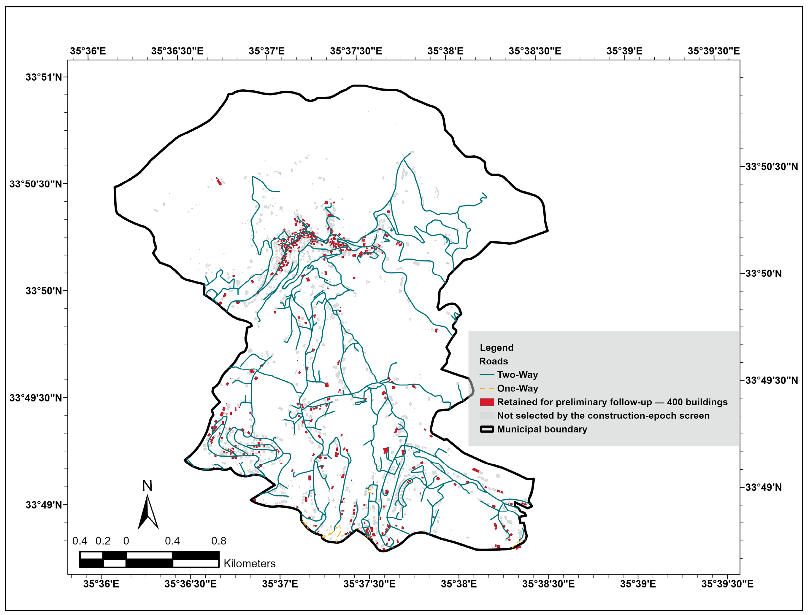
The retained product is deliberately modest: 400 pre-1990 buildings for preliminary follow-up (Figure 14). Municipal staff could use the queue to organize records review, field reconnaissance, and engineering inspection. They should not use it to infer safety, occupancy restrictions, retrofitting needs, or expected damage without further evidence. Buildings outside the queue are not “safe,” and buildings inside it are not predicted failures.
The audit also identifies where resources could improve the decision system. A structured building survey, such as the rapid visual screening protocols applied at the urban scale elsewhere, would strengthen the age proxy and add direct structural attributes [43,44,47]. Local site characterization would allow a ground-condition layer to be built on the measured evidence. A fully scripted and preserved raster environment would allow a newly reconstructed Newmark and ERI processing chain to be evaluated against the gates [18]. That rerun would be a transparent new candidate, not retroactive proof that the rejected project raster had the same provenance.
The queue carries no structural information: no structural system, material properties, infill-wall configuration, or soil–structure interaction (SSI), and no capacity value. Downstream engineering assessment must account for these explicitly, since neglecting infill walls and SSI can materially influence seismic response and bias capacity estimates [94].

4.10. Limitations of the Study

This study has several limitations. First, EGS was applied to one municipality and one project archive. Four external products were assessed independently by two assessors who took no part in the study. This tests whether the admission logic can be applied consistently outside that archive. Four purposively selected cases do not establish transferability to other jurisdictions, datasets, or decision domains. The epoch boundaries are tied to Lebanese seismic-code milestones and to local construction history, and would require re-derivation elsewhere. No observed earthquake-damage inventory was available, so the retained queue was not validated against structural performance. The output should be read only as a preliminary inspection-prioritization tool.
Second, the available evidence limits several candidates. The construction-epoch proxy lacks historical imagery between 1985 and 2001. The intermediate 1990–2000 class could not be resolved and the proxy operates as a binary pre-1990 indicator. Also, some reference labels rest on respondent recall. The soil analysis lacks local VS30, borehole, or geophysical observations, and the archive records no rationale for the reduction from three source classes to two building classes. Parts of the Newmark and ERI chains have incomplete provenance. Raster-to-building transfer omitted 270 footprints, although this affected the rejected chain rather than the retained queue.
Third, the gate criteria were fixed before the admission decisions but were not preregistered before the historical workflow was built. The conditional-admission thresholds were made explicit for this case but were not externally calibrated, and the 30 cm class was a project threshold, and not a standard.
Fourth, admission decisions are specific to the evidence available when they are made. New construction, demolition, revised footprints, or updated remote-sensing products alter the evidence base underlying a gate. Decisions therefore require documented versioning and periodic re-evaluation rather than standing indefinitely. Deployment beyond a single municipality would also require benchmarking the audit procedure itself, particularly the raster-to-building transfer and the bootstrap validation.
Finally, EGS is a screening framework. It does not model structural system, material properties, condition, soil–structure interaction, capacity, damage, or failure probability. The reported confidence intervals characterize sampling uncertainty in the validation of the construction-epoch proxy. They are not the seismic-risk uncertainty for individual buildings, and they are not building-level confidence scores.

4.11. Transferability and Future Research

EGS applies to other GIS applications in which heterogeneous evidence is fused. These include flood prioritization, landslide screening, public-health accessibility, conservation planning, and infrastructure maintenance, domains where multi-criteria overlay is already routine [9]. The four gate questions do not change between applications. Admission thresholds and hard-failure rules must be defined for each decision context. A transferable application follows five steps: (1) define the decision use, decision unit, and prohibited interpretations; (2) declare hard-failure conditions and conditional-admission criteria before interpreting candidate results; (3) audit every candidate independently under G1–G4; (4) freeze the evidence trail and quantify the counterfactual consequence of retaining or rejecting each layer; and (5) fuse only layers admitted for the same purpose and decision unit. Municipalities may adopt different numerical thresholds. Those thresholds should be declared before the results are seen and justified by the decision consequences, not read off the observed results.
The external verification in Section 3.10 tests this claim only partially: there were two assessors, four products, and no repeated trials across jurisdictions. A general claim would require the same gates to be applied to further products, decision domains, and independent assessor pairs.
The exercise also exposed a gap in the admission rules. It mattered in the one external case whose source both limits the declared use and describes a permitted use at the same decision unit. The rule as written did not determine which reading was correct. A workable definition would likely turn on whether the source itself states a use at the declared decision unit, but establishing that requires cases beyond the four assessed here.
Validation of an assessment procedure accumulates evidence supporting a specific interpretation and use. A single comparison against a known-correct classification does not establish it [74]. Criterion validity would require a corpus of products whose fitness for stated decisions is known independently of any admission procedure. No such corpus exists for geospatial fitness-for-use. Building one, even for a narrow class of decisions, would be a useful contribution in its own right.
The next step is an independently designed building survey. It should verify construction period together with the structural material, structural system, story count, irregularity, apparent condition, occupancy, and retrofit history [43,44,47]. Local VS30, borehole, or geophysical observations are needed before a soil-based site-response layer can be reconsidered. Replication by an independent team in another municipality would test whether EGS decisions reproduce under different data constraints [17], applying preregistered gate rules.

5. Conclusions

EGS answered the research questions posed at each gate by separating reproducibility, applicability, signal validity, and input support before spatial fusion. The construction-epoch workflow was recoverable and retained useful binary discrimination, but its stratified 216-building validation was constrained by the absence of historical imagery between 1985 and 2001 and supported only conditional, low-consequence use. The building-level soil criterion was reproducible yet failed in terms of applicability and input support. The project Newmark implementation failed raw-generator reconstruction, showed substantial calibration-domain violations, and contained no valid in-domain prediction in its 30 cm class. The ERI passed formula-level reconstruction but failed at the component and input-chain level and inherited the limitations of its inputs.
Only the construction-epoch proxy was conditionally admitted. The retained output is a preliminary inspection queue of 400 pre-1990 buildings. It is not a vulnerability map, damage estimate, failure probability, or statement of structural safety. Relative to the exploratory ASI overlay, pre-fusion evidence admission increased the queue by 97 buildings. It also isolated 58 inadmissible units in the 30 cm Newmark class, all of them caps or below-domain extrapolations, and 270 buildings omitted by historical raster transfer. Each of these consequences follows from an admission rule declared before the results were examined, not from a preference among outcomes.
Four external products were assessed by two assessors from outside the study. They agreed on 13 of 16 gate outcomes and on all four dispositions, and their recorded reasoning matched the applicability limitation each source states in its own words, including on the three gates where their recorded status differed. The exercise also showed that the term “material”, which separates a rejection at G2 from a conditional pass, is not operationally defined. Defining it is a prerequisite for applying the gates outside a single archive.
The case supports EGS as an auditable evidence-governance procedure. It does not validate the retained queue as a predictor of seismic performance. The framework’s transferable claim is narrower and stronger than a screening result: reproducibility, applicability, signal validity, and input support are separable properties, and a layer may satisfy any one of them while failing another. Whether the framework performs consistently across other jurisdictions, datasets, and decision domains remains untested and requires independent multi-site validation.

Supplementary Materials

The following supporting information can be downloaded at: https://www.mdpi.com/article/doi/s1, Text S1: Digital elevation model and building inventory; Text S2: Soil and geotechnical parameterization; Text S3: Age-Soil Index (ASI); Text S4: Newmark processing chain; Text S5: Earthquake Risk Index (ERI) component preparation; Figure S1: Digital elevation model of Aabadiyeh Municipality; Figure S2: Slope map; Figure S3: Municipal building inventory; Figure S4: Exploratory building-level ASI classes; Figure S5: Newmark-displacement status at the historical 30 cm threshold; Figure S6: Critical-acceleration applicability classes; Figure S7: Project-specific raster ERI classes; Figure S8: Building-level calibration-domain support; Equation (S1): Dry unit weight; Equation (S2): Effective source-to-site distance; Equation (S3): Arias-intensity relation; Equation (S4): Newmark displacement relation; Table S1: Source, spatial support, workflow, and verification inventory; Table S2: Construction-epoch validation metrics; Table S3a: Validation sampling design; Table S3b: Per-record validation data; Table S3c: Inter-rater agreement; Table S3d: Post-stratified municipal estimates; Table S3e: Sensitivity of validation accuracy to evidence quality; Table S3f: Field-verification summary; Table S4: Source-side to building-level soil-class crosswalk; Table S5: Factor-of-safety reconstruction audit; Table S6: Post-processing, mask, grid, and deterministic-comparison audit; Table S7: Calibration-domain and threshold cross-tabulations; Table S8: Raster-to-building transfer omission audit; Table S8a: Morphology of omitted and retained footprints; Table S8b: Omission by construction-epoch class; Table S8c: Omission test battery; Table S8d: Omission-analysis input table; Table S8e: Re-execution of the archived raster-to-building transfer; Table S9: Figure source inventory; Table S10a: External reference-case verification protocol and consent summary; Table S10b: External reference-case gate-by-gate records; Table S11: Candidate class codes and measurement scales. Tables S1–S11 are provided in a single supplementary workbook. The preservation package additionally includes processing scripts, environment documentation, a data dictionary, workflow notes, and checksums for redistributable audit files.

Author Contributions

Conceptualization, Mervana Mograby and Amal Iaaly; methodology, Mervana Mograby and Amal Iaaly; software, Mervana Mograby; validation, Mervana Mograby and Amal Iaaly; formal analysis, Mervana Mograby; investigation, Mervana Mograby; resources, Mervana Mograby and Amal Iaaly; data curation, Mervana Mograby and Amal Iaaly; writing—original draft preparation, Mervana Mograby and Amal Iaaly; writing—review and editing, Mervana Mograby and Amal Iaaly; visualization, Mervana Mograby; supervision, Amal Iaaly. All authors have read and agreed to the published version of the manuscript.

Funding

This research received no external funding. The University of Balamand provided routine institutional access to computing facilities and project storage. No external grant supported the study, and no external sponsor had a role in the study design, analysis, interpretation, manuscript preparation, or decision to submit.

Institutional Review Board Statement

The Institutional Review Board of the University of Balamand exempted this research from review on 7 September 2026 (Project Reference No. UOB/IRB/2026/066). The exemption applies to the three components involving human subjects or human-derived data: the Google Earth historical-imagery interpretation, the field data collection on building construction year, and the external reference-case verification.

Informed Consent Statement

Informed consent was obtained from all respondents prior to participation; respondents were advised of the purpose of the study, the information recorded and the intended publication of aggregated results, and that participation was voluntary. No personally identifying information was recorded.

Data Availability Statement

GAIA Version 2024 (1985–2024) is publicly documented and distributed under CC BY 4.0 through the dataset record, DOI:10.6084/m9.figshare.27245775 (accessed 18 July 2026) [31]. HWSD version 2.0 is publicly documented by the Food and Agriculture Organization of the United Nations (FAO) and the International Institute for Applied Systems Analysis (IIASA) [33], and the lookup table between the United States Department of Agriculture (USDA) soil classification and the Unified Soil Classification System (USCS) is available from the U.S. Army Engineer Research and Development Center, Cold Regions Research and Engineering Laboratory (ERDC/CRREL) [34]. The aggregate building counts, gate decisions, confusion matrices, bootstrap summaries, factor-of-safety diagnostics, calibration-domain tables, threshold cross-tabulations, raster-transfer omission ledger, scripts, environment notes, data dictionary, and available checksums accompany the submission. Municipal building geometry, detailed institutional soil polygons, the project digital elevation model, and project rasters are not redistributed because public-release permission is not established. Controlled scholarly verification may be requested from the corresponding author, subject to the data owners’ written permission and any required data-use agreement.

Acknowledgments

The authors acknowledge the GIS Center at the University of Balamand for computational and institutional support. The authors remain responsible for the numerical checks, interpretations, and conclusions. During preparation of this manuscript, the authors used OpenAI ChatGPT version 5.6 (accessed 18 July 2026) for minimal language editing, structural organization, code review, and refinement of explanatory text, captions, and tables. The tool was not used as an autonomous source of data or evidence. The authors checked all numerical values, equations, citations, figures, and interpretations against the project record and cited sources, reviewed and edited the resulting text, and take full responsibility for the publication.

Conflicts of Interest

The authors declare no conflicts of interest.

Appendix A. Equations Referenced in the Main Text

FS = c/(γd z sin α cos α) + [(1 − ru) tan φ]/tan α,
where FS is the dimensionless factor of safety, c is cohesion (kPa), γd is dry unit weight (kN m−3), z is slab thickness (m; intended value 2.4 m), α is slope angle (degrees), ru is the dimensionless pore-pressure ratio, and φ is friction angle (degrees). The parameter values are regional literature-based proxies whose derivation is described in Supplementary Text S2, Equation (S1).
ac = max [0, (FS − 1) sin α],
where ac is the critical (yield) acceleration normalized by gravitational acceleration and reported in units of g, and FS and α are as defined for Equation (A1).

References

  1. Armaş, I.; Toma-Danila, D.; Ionescu, R.; Gavriş, A. Vulnerability to earthquake hazard: Bucharest case study, Romania. Int. J. Disaster Risk Sci. 2017, 8, 182–195. [Google Scholar] [CrossRef] [Scilit]
  2. Xofi, M.; Domingues, J.C.; Santos, P.; Pereira, S.; Oliveira, S.; Reis, E.; Zêzere, J.; Garcia, R.A.C.; Lourenço, P.; Ferreira, T. Exposure and physical vulnerability indicators to assess seismic risk in urban areas: A step towards a multi-hazard risk analysis. Geomat. Nat. Hazards Risk 2022, 13, 1154–1177. [Google Scholar] [CrossRef] [Scilit]
  3. Leggieri, V.; Mastrodonato, G.; Uva, G. GIS multisource data for the seismic vulnerability assessment of buildings at the urban scale. Buildings 2022, 12, 523. [Google Scholar] [CrossRef] [Scilit]
  4. Grigoratos, I.; Monteiro, R.; Ceresa, P.; Di Meo, A.; Faravelli, M.; Borzi, B. Crowdsourcing exposure data for seismic vulnerability assessment in developing countries. J. Earthq. Eng. 2021, 25, 835–852. [Google Scholar] [CrossRef] [Scilit]
  5. Jena, R.; Pradhan, B.; Beydoun, G. Earthquake vulnerability assessment in Northern Sumatra Province by using a multi-criteria decision-making model. Int. J. Disaster Risk Reduct. 2020, 46, 101518. [Google Scholar] [CrossRef] [Scilit]
  6. Alizadeh, M.; Hashim, M.; Alizadeh, E.; Shahabi, H.; Karami, M.; Pour, A.B.; Pradhan, B.; Zabihi, H. Multi-criteria decision making model for seismic vulnerability assessment of urban residential buildings. ISPRS Int. J. Geo-Inf. 2018, 7, 444. [Google Scholar] [CrossRef] [Scilit]
  7. Saaty, T.L. The Analytic Hierarchy Process: Planning, Priority Setting, Resource Allocation; McGraw-Hill: New York, NY, USA, 1980. [Google Scholar]
  8. Panahi, M.; Rezaie, F.; Meshkani, S.A. Seismic vulnerability assessment of school buildings in Tehran city based on AHP and GIS. Nat. Hazards Earth Syst. Sci. 2014, 14, 969–979. [Google Scholar] [CrossRef] [Scilit]
  9. Malczewski, J. GIS-based multicriteria decision analysis: A survey of the literature. Int. J. Geogr. Inf. Sci. 2006, 20, 703–726. [Google Scholar] [CrossRef] [Scilit]
  10. Feizizadeh, B.; Jankowski, P.; Blaschke, T. GIS-based spatially explicit sensitivity and uncertainty analysis approach for multi-criteria decision analysis. Comput. Geosci. 2014, 64, 81–95. [Google Scholar] [CrossRef] [Scilit] [PubMed]
  11. ISO 19157-1:2023; Geographic Information—Data Quality—Part 1: General Requirements. ISO: Geneva, Switzerland, 2023.
  12. Devillers, R.; Jeansoulin, R. (Eds.) Fundamentals of Spatial Data Quality; ISTE: London, UK, 2006. [Google Scholar]
  13. Devillers, R.; Bédard, Y.; Jeansoulin, R.; Moulin, B. Towards spatial data quality information analysis tools for experts assessing the fitness for use of spatial data. Int. J. Geogr. Inf. Sci. 2007, 21, 261–282. [Google Scholar] [CrossRef] [Scilit]
  14. Moreau, L.; Missier, P. (Eds.) PROV-DM: The PROV Data Model. W3C Recommendation 30 April 2013. Available online: https://www.w3.org/TR/prov-dm/ (accessed on 16 July 2026).
  15. Forkan, A.; Both, A.; Bellman, C.; Duckham, M.; Anderson, H.; Radosevic, N. K-Span: Open and reproducible spatial analytics using scientific workflows. Front. Earth Sci. 2023, 11, 1130262. [Google Scholar] [CrossRef] [Scilit]
  16. Scheip, C.; Wegmann, K. HazMapper: A global open-source natural hazard mapping application in Google Earth Engine. Nat. Hazards Earth Syst. Sci. 2021, 21, 1495–1511. [Google Scholar] [CrossRef] [Scilit]
  17. Kedron, P.; Li, W.; Fotheringham, A.S.; Goodchild, M.F. Reproducibility and replicability: Opportunities and challenges for geospatial research. Int. J. Geogr. Inf. Sci. 2021, 35, 427–445. [Google Scholar] [CrossRef] [Scilit]
  18. Wilson, J.P.; Butler, K.; Gao, S.; Hu, Y.; Li, W.; Wright, D.J. A five-star guide for achieving replicability and reproducibility when working with GIS software and algorithms. Ann. Am. Assoc. Geogr. 2021, 111, 1311–1317. [Google Scholar] [CrossRef] [Scilit]
  19. Wagner, M.; Henzen, C. Quality assurance for spatial research data. ISPRS Int. J. Geo-Inf. 2022, 11, 334. [Google Scholar] [CrossRef] [Scilit]
  20. Brodeur, J.; Coetzee, S.; Danko, D.; Garcia, S.; Hjelmager, J. Geographic information metadata—An outlook from the international standardization perspective. ISPRS Int. J. Geo-Inf. 2019, 8, 280. [Google Scholar] [CrossRef] [Scilit]
  21. Nawaz, M.; Kalisa, W.; Zaheen, Z.; Tauqir, M.; Zhang, J.; Shah, A.A.; Ullah, K. Spatiotemporal Assessment of Desertification Sensitivity in Ningxia, China, Using the MEDALUS Framework and Random Forest Classification (2001–2022). J. Geosci. Earth Obs. 2026, 1, 39–54. [Google Scholar] [CrossRef] [Scilit]
  22. El Kadri, S.; Beauval, C.; Brax, M.; Bard, P.-Y.; Vergnolle, M.; Klinger, Y. A fault-based probabilistic seismic hazard model for Lebanon, controlling parameters and hazard levels. Bull. Earthq. Eng. 2023, 21, 3163–3197. [Google Scholar] [CrossRef] [Scilit]
  23. Daëron, M.; Klinger, Y.; Tapponnier, P.; Elias, A.; Jacques, E.; Sursock, A. 12,000-year-long record of 10 to 13 paleoearthquakes on the Yammouneh Fault, Levant Fault System, Lebanon. Bull. Seismol. Soc. Am. 2007, 97, 749–771. [Google Scholar] [CrossRef] [Scilit]
  24. Styron, R.; Pagani, M. The GEM Global Active Faults Database. Earthq. Spectra 2020, 36, 160–180. [Google Scholar] [CrossRef] [Scilit]
  25. Grigoratos, I.; Poggi, V.; Danciu, L.; Monteiro, R. Homogenizing instrumental earthquake catalogs—A case study around the Dead Sea Transform Fault Zone. Seismica 2023, 2, 402. [Google Scholar] [CrossRef] [Scilit]
  26. Grigoratos, I.; Poggi, V.; Danciu, L. A Homogenized Instrumental Earthquake Catalog Around the Dead Sea Transform Fault Zone [Data Set]; ISC Seismological Dataset Repository; ISC: Berkshire, UK, 2023. [Google Scholar] [CrossRef] [Scilit]
  27. U.S. Geological Survey, Earthquake Hazards Program. ANSS Comprehensive Earthquake Catalog (ComCat) [Data Set]. FDSN Event Web Service. Available online: https://earthquake.usgs.gov/fdsnws/event/1/ (accessed on 4 September 2026).
  28. Microsoft. GlobalMLBuildingFootprints: Worldwide Building Footprints Derived from Satellite Imagery, 2023 Release; Microsoft: Redmond, WA, USA, 2023; Available online: https://github.com/microsoft/GlobalMLBuildingFootprints (accessed on 19 March 2026).
  29. Esri. World Imagery; Esri: Redlands, CA, USA, 2025; Available online: https://www.arcgis.com/home/item.html?id=10df2279f9684e4a9f6a7f08febac2a9 (accessed on 21 March 2026).
  30. Gong, P.; Li, X.; Wang, J.; Bai, Y.; Chen, B.; Hu, T.; Liu, X.; Xu, B.; Yang, J.; Zhang, W.; et al. Annual maps of global artificial impervious area (GAIA) between 1985 and 2018. Remote Sens. Environ. 2020, 236, 111510. [Google Scholar] [CrossRef] [Scilit]
  31. Gong, P. Global Artificial Impervious Area (GAIA), Version 2024 [Data Set]; Figshare: London, UK, 2024. [Google Scholar] [CrossRef]
  32. CNRS Center for Remote Sensing. Detailed Soil Map of Lebanon, 1:50,000; 27 Map Sheets and Explanatory Documentation; National Council for Scientific Research (CNRS): Beirut, Lebanon; National Center for Remote Sensing (NCRS): Beirut, Lebanon, 1997–2006. [Google Scholar]
  33. Food and Agriculture Organization of the United Nations; International Institute for Applied Systems Analysis. Harmonized World Soil Database Version 2.0; FAO: Rome, Italy, 2023. [Google Scholar] [CrossRef] [Scilit]
  34. García-Gaines, R.A.; Frankenstein, S. USCS and the USDA Soil Classification System: Development of a Mapping Scheme; ERDC/CRREL TR-15-4; U.S. Army Engineer Research and Development Center: Hanover, NH, USA, 2015. Available online: https://hdl.handle.net/11681/5485 (accessed on 20 March 2026).
  35. Newmark, N.M. Effects of earthquakes on dams and embankments. Géotechnique 1965, 15, 139–160. [Google Scholar] [CrossRef] [Scilit]
  36. Jibson, R.W. Predicting earthquake-induced landslide displacements using Newmark’s sliding block analysis. Transp. Res. Rec. 1993, 1411, 9–17. [Google Scholar]
  37. Jibson, R.W.; Harp, E.L.; Michael, J.A. A Method for Producing Digital Probabilistic Seismic Landslide Hazard Maps: An Example from the Los Angeles, California, Area; Open-File Report 98-113; U.S. Geological Survey: Reston, VA, USA, 1998. [CrossRef] [Scilit]
  38. Jibson, R.W.; Harp, E.L.; Michael, J.A. A method for producing digital probabilistic seismic landslide hazard maps. Eng. Geol. 2000, 58, 271–289. [Google Scholar] [CrossRef] [Scilit]
  39. Arias, A. A measure of earthquake intensity. In Seismic Design for Nuclear Power Plants; Hansen, R.J., Ed.; MIT Press: Cambridge, MA, USA, 1970; pp. 438–483. [Google Scholar]
  40. Travasarou, T.; Bray, J.D.; Abrahamson, N.A. Empirical attenuation relationship for Arias intensity. Earthq. Eng. Struct. Dyn. 2003, 32, 1133–1155. [Google Scholar] [CrossRef] [Scilit]
  41. Johnson, K.; Villani, M.; Bayliss, K.; Brooks, C.; Chandrasekhar, S.; Chartier, T.; Chen, Y.; Garcia-Pelaez, J.; Gee, R.; Styron, R.; et al. Global Earthquake Model (GEM) Seismic Hazard Map (Version 2023.1—June 2023); Zenodo: Geneva, Switzerland, 2023. [Google Scholar] [CrossRef]
  42. Pagani, M.; Garcia-Pelaez, J.; Gee, R.; Johnson, K.; Poggi, V.; Silva, V.; Simionato, M.; Styron, R.; Viganò, D.; Danciu, L.; et al. The 2018 version of the Global Earthquake Model: Hazard component. Earthq. Spectra 2020, 36, 226–251. [Google Scholar] [CrossRef] [Scilit]
  43. Kassem, M.; Beddu, S.; Ooi, J.; Tan, C.; El-Maissi, A.M.; Nazri, M.F. Assessment of seismic building vulnerability using rapid visual screening through a web-based application for Malaysia. Buildings 2021, 11, 485. [Google Scholar] [CrossRef] [Scilit]
  44. Ahmed, S.; Abarca, A.; Perrone, D.; Monteiro, R. Large-scale seismic assessment of reinforced-concrete buildings through rapid visual screening. Int. J. Disaster Risk Reduct. 2022, 80, 103219. [Google Scholar] [CrossRef] [Scilit]
  45. Gerçek, D.; Güven, I.T. Urban earthquake vulnerability assessment and mapping at the microscale based on the catastrophe progression method. Int. J. Disaster Risk Sci. 2023, 14, 768–781. [Google Scholar] [CrossRef] [Scilit]
  46. Negulescu, C.; Smai, F.; Quique, R.; Hohmann, A.; Clain, U.; Guidez, R.; Tellez-Arenas, A.; Quentin, A.; Grandjean, G. VIGIRISKS platform, a web tool for single- and multi-hazard risk assessment. Nat. Hazards 2023, 115, 593–618. [Google Scholar] [CrossRef] [Scilit]
  47. Rajarathnam, S.; Santhakumar, A.R. Assessment of seismic building vulnerability based on rapid visual screening technique aided by aerial photographs on a GIS platform. Nat. Hazards 2015, 78, 779–802. [Google Scholar] [CrossRef] [Scilit]
  48. Zhuo, L.; Huang, R.; Liao, C.; Tao, H.; Zang, Y. BATSCCD: A new change detection method for mapping building age in rapidly changing urban areas using Landsat time series data. Int. J. Digit. Earth 2024, 17, 2358859. [Google Scholar] [CrossRef] [Scilit]
  49. Hu, T.; Zhang, M.; Li, X.; Wu, T.; Ma, Q.; Xiao, J.; Huang, X.; Guo, J.; Li, Y.; Liu, D. Extraction of Building Construction Time Using the LandTrendr Model with Monthly Landsat Time Series Data. IEEE J. Sel. Top. Appl. Earth Obs. Remote Sens. 2024, 17, 18335–18350. [Google Scholar] [CrossRef] [Scilit]
  50. Yu, W.; Jing, C.; Zhou, W.; Wang, W.; Zheng, Z. Time-Series Landsat Data for 3D Reconstruction of Urban History. Remote Sens. 2021, 13, 4339. [Google Scholar] [CrossRef] [Scilit]
  51. Jie, N.; Zhuo, L.; Li, Q.; Tao, H. An Enhanced Hierarchical Framework for Mapping Urban Building Age Using Long-Term Landsat Time-Series Imagery. IEEE J. Sel. Top. Appl. Earth Obs. Remote Sens. 2026, 19, 13081–13096. [Google Scholar] [CrossRef] [Scilit]
  52. Biljecki, F.; Sindram, M. Estimating building age with 3D GIS. ISPRS Ann. Photogramm. Remote Sens. Spat. Inf. Sci. 2017, IV-4/W5, 17–24. [Google Scholar] [CrossRef] [Scilit]
  53. Dionelis, N.; Longépé, N.; Feliciotti, A.; Marconcini, M.; Peressutti, D.; Oman Kadunc, N.; Park, J.; Raja Sinulingga, H.; Immanuel, S.A.; Tran, B.-C.; et al. Building Age Estimation: A New Multi-Modal Benchmark Dataset and Community Challenge. arXiv 2025, arXiv:2502.13818. [Google Scholar] [CrossRef] [Scilit]
  54. Uhl, J.H.; Leyk, S. Towards a novel backdating strategy for creating built-up land time series data using contemporary spatial constraints. Remote Sens. Environ. 2020, 238, 111197. [Google Scholar] [CrossRef] [Scilit]
  55. Liu, Y.; Zhang, X.; Mo, Z.; Wang, Z.; Zhang, Q. Mapping Building Construction Year from Landsat in Data-Scarce, Cloud-Prone Regions: A Parsimonious Spatial Triage Tool for Physical Vulnerability Screening. Remote Sens. 2026, 18, 2135. [Google Scholar] [CrossRef] [Scilit]
  56. Yepes-Estrada, C.; Calderon, A.; Costa, C.; Crowley, H.; Dabbeek, J.; Hoyos, M.C.; Martins, L.; Paul, N.; Rao, A.; Silva, V. Global building exposure model for earthquake risk assessment. Earthq. Spectra 2023, 39, 2212–2235. [Google Scholar] [CrossRef] [Scilit]
  57. Jibson, R.W. Regression models for estimating coseismic landslide displacement. Eng. Geol. 2007, 91, 209–218. [Google Scholar] [CrossRef] [Scilit]
  58. Adeniyi, O.D.; Maerker, M. Explorative analysis of varying spatial resolutions on a soil type classification model and its transferability in an agricultural lowland area of Lombardy, Italy. Geoderma Reg. 2024, 37, e00785. [Google Scholar] [CrossRef] [Scilit]
  59. Teng, H.; Viscarra Rossel, R.A.; Shi, Z.; Behrens, T. Updating a national soil classification with spectroscopic predictions and digital soil mapping. Catena 2018, 164, 125–134. [Google Scholar] [CrossRef] [Scilit]
  60. Rizzo, R.; Medeiros, L.G.; de Mello, D.C.; Marques, K.P.P.; Mendes, W.d.S.; Quiñonez Silvero, N.E.; Dotto, A.C.; Bonfatti, B.R.; Demattê, J.A.M. Multi-temporal bare surface image associated with transfer functions to support soil classification and mapping in southeastern Brazil. Geoderma 2020, 361, 114018. [Google Scholar] [CrossRef] [Scilit]
  61. Chousianitis, K.; Del Gaudio, V.; Kalogeras, I.; Ganas, A. Predictive model of Arias intensity and Newmark displacement for regional-scale evaluation of earthquake-induced landslide hazard in Greece. Soil Dyn. Earthq. Eng. 2014, 65, 11–29. [Google Scholar] [CrossRef] [Scilit]
  62. Zhang, Y.; Zhao, H.; Long, Y. CMAB: A Multi-Attribute Building Dataset of China. Sci. Data 2025, 12, 430. [Google Scholar] [CrossRef] [Scilit] [PubMed]
  63. Poggio, L.; de Sousa, L.M.; Batjes, N.H.; Heuvelink, G.B.M.; Kempen, B.; Ribeiro, E.; Rossiter, D. SoilGrids 2.0: Producing soil information for the globe with quantified spatial uncertainty. SOIL 2021, 7, 217–240. [Google Scholar] [CrossRef] [Scilit]
  64. ISRIC—World Soil Information. SoilGrids FAQ. 2023. Available online: https://docs.isric.org/globaldata/soilgrids/SoilGrids_faqs_04.html (accessed on 3 September 2026).
  65. Mirus, B.B.; Belair, G.M.; Wood, N.J.; Jones, J.; Martinez, S.N. Parsimonious High-Resolution Landslide Susceptibility Modeling at Continental Scales. AGU Adv. 2024, 5, e2024AV001214. [Google Scholar] [CrossRef] [Scilit]
  66. Lebanon Joint Analysis Unit. INFORM Subnational Risk Index Lebanon 2024, v1.0; European Commission Joint Research Centre, Disaster Risk Management Knowledge Centre: Ispra, Italy, 2024; Available online: https://drmkc.jrc.ec.europa.eu/inform-index/INFORM-Subnational-Risk/Lebanon (accessed on 1 July 2026).
  67. Marin-Ferrer, M.; Vernaccini, L.; Poljansek, K. Index for Risk Management—INFORM: Concept and Methodology, Version 2017; EUR 28655 EN, JRC106949; Publications Office of the European Union: Luxembourg, 2017. [Google Scholar] [CrossRef]
  68. Garschagen, M.; Doshi, D.; Reith, J.; Hagenlocher, M. Global patterns of disaster and climate risk—An analysis of the consistency of leading index-based assessments and their results. Clim. Change 2021, 169, 11. [Google Scholar] [CrossRef] [Scilit]
  69. Birkmann, J.; Jamshed, A.; McMillan, J.M.; Feldmeyer, D.; Totin, E.; Solecki, W.; Ibrahim, Z.Z.; Roberts, D.; Bezner Kerr, R.; Poertner, H.-O.; et al. Understanding human vulnerability to climate change: A global perspective on index validation for adaptation planning. Sci. Total Environ. 2022, 803, 150065. [Google Scholar] [CrossRef] [Scilit] [PubMed]
  70. Petutschnig, L.; Clemen, T.; Klaüßner, E.S.; Clemen, U.; Lang, S. Evaluating Geospatial Data Adequacy for Integrated Risk Assessments: A Malaria Risk Use Case. ISPRS Int. J. Geo-Inf. 2024, 13, 33. [Google Scholar] [CrossRef] [Scilit]
  71. Jonietz, D.; Zipf, A. Defining Fitness-for-Use for Crowdsourced Points of Interest (POI). ISPRS Int. J. Geo-Inf. 2016, 5, 149. [Google Scholar] [CrossRef] [Scilit]
  72. Homburg, T. Connecting Semantic Situation Descriptions with Data Quality Evaluations—Towards a Framework of Automatic Thematic Map Evaluation. Information 2020, 11, 532. [Google Scholar] [CrossRef] [Scilit]
  73. Degrossi, L.C.; Porto de Albuquerque, J.; dos Santos Rocha, R.; Zipf, A. A taxonomy of quality assessment methods for volunteered and crowdsourced geographic information. Trans. GIS 2018, 22, 542–560. [Google Scholar] [CrossRef] [Scilit] [PubMed]
  74. Cook, D.A.; Brydges, R.; Ginsburg, S.; Hatala, R. A contemporary approach to validity arguments: A practical guide to Kane’s framework. Med. Educ. 2015, 49, 560–575. [Google Scholar] [CrossRef] [Scilit] [PubMed]
  75. Lebanese Republic. Decree No. 11266: Conditions and Technical Specifications to Be Followed for Design and Construction of Anti-Seismic Structures; Government of Lebanon: Beirut, Lebanon, 1997. [Google Scholar]
  76. Lebanese Republic. Decree No. 14293: Requirements and Conditions for Buildings, Installations, and Elevators for the Protection Against Fires and Earthquakes; Government of Lebanon: Beirut, Lebanon, 2005.
  77. Lebanese Republic. Decree No. 7964: Public Safety Law, Amending Decree No. 14293 of 2005 Regarding Seismic Risk Parameters; Government of Lebanon: Beirut, Lebanon, 2012.
  78. Zhang, X.; Liu, L.; Zhao, T.; Gao, Y.; Chen, X.; Mi, J. GISD30: Global 30 m impervious-surface dynamic dataset from 1985 to 2020 using time-series Landsat imagery on the Google Earth Engine platform. Earth Syst. Sci. Data 2022, 14, 1831–1856. [Google Scholar] [CrossRef] [Scilit]
  79. Olofsson, P.; Foody, G.M.; Herold, M.; Stehman, S.V.; Woodcock, C.E.; Wulder, M.A. Good practices for estimating area and assessing accuracy of land change. Remote Sens. Environ. 2014, 148, 42–57. [Google Scholar] [CrossRef] [Scilit]
  80. Stehman, S.V.; Foody, G.M. Key issues in rigorous accuracy assessment of land cover products. Remote Sens. Environ. 2019, 231, 111199. [Google Scholar] [CrossRef] [Scilit]
  81. Foody, G.M. Explaining the unsuitability of the kappa coefficient in the assessment and comparison of the accuracy of thematic maps obtained by image classification. Remote Sens. Environ. 2020, 239, 111630. [Google Scholar] [CrossRef] [Scilit]
  82. IUSS Working Group WRB. World Reference Base for Soil Resources; International Soil Classification System for Naming Soils and Creating Legends for Soil Maps, 4th ed.; International Union of Soil Sciences (IUSS): Vienna, Austria, 2022. [Google Scholar]
  83. Gupta, K.; Satyam, N. Co-seismic landslide hazard assessment of Uttarakhand State (India) based on the modified Newmark model. J. Asian Earth Sci. X 2022, 8, 100120. [Google Scholar] [CrossRef] [Scilit]
  84. Li, Y.; Ming, D.; Zhang, L.; Niu, Y.; Chen, Y. Seismic landslide susceptibility assessment using Newmark displacement based on a dual-channel convolutional neural network. Remote Sens. 2024, 16, 566. [Google Scholar] [CrossRef] [Scilit]
  85. Fischer, J.; Egli, L.; Groth, J.; Barrasso, C.; Ehrmann, S.; Figgemeier, H.; Henzen, C.; Meyer, C.; Müller-Pfefferkorn, R.; Rümmler, A.; et al. Approaches and tools for user-driven provenance and data quality information in spatial data infrastructures. Int. J. Digit. Earth 2023, 16, 1510–1529. [Google Scholar] [CrossRef] [Scilit]
  86. Powell, R.L.; Matzke, N.; de Souza, C.; Clark, M.; Numata, I.; Hess, L.L.; Roberts, D.A. Sources of error in accuracy assessment of thematic land-cover maps in the Brazilian Amazon. Remote Sens. Environ. 2004, 90, 221–234. [Google Scholar] [CrossRef] [Scilit]
  87. Pengra, B.W.; Stehman, S.V.; Horton, J.A.; Dockter, D.J.; Schroeder, T.A.; Yang, Z.; Cohen, W.B.; Healey, S.P.; Loveland, T.R. Quality control and assessment of interpreter consistency of annual land cover reference data in an operational national monitoring program. Remote Sens. Environ. 2020, 238, 111261. [Google Scholar] [CrossRef] [Scilit]
  88. McRoberts, R.E.; Stehman, S.V.; Liknes, G.C.; Næsset, E.; Sannier, C.; Walters, B.F. The effects of imperfect reference data on remote sensing-assisted estimators of land cover class proportions. ISPRS J. Photogramm. Remote Sens. 2018, 142, 292–300. [Google Scholar] [CrossRef] [Scilit]
  89. Shimizu, K.; Saito, H.; Furuta, T.; Sasakawa, H.; Seto, T.; Mai, K.; Kanamori, C.; Hirano, A.; Kanemoto, N. Quantifying consistency among interpreters of reference data for estimation of harvest area through visual interpretation of remote sensing data. Forestry 2026, 99, cpaf077. [Google Scholar] [CrossRef] [Scilit]
  90. Cohen, J. A coefficient of agreement for nominal scales. Educ. Psychol. Meas. 1960, 20, 37–46. [Google Scholar] [CrossRef] [Scilit]
  91. Gotway, C.A.; Young, L.J. Combining incompatible spatial data. J. Am. Stat. Assoc. 2002, 97, 632–648. [Google Scholar] [CrossRef] [Scilit]
  92. Boehm, B.W. Software Engineering Economics; Prentice-Hall: Englewood Cliffs, NJ, USA, 1981. [Google Scholar]
  93. Li, W.; Hsu, C.-Y.; Wang, S.; Kedron, P. GeoAI reproducibility and replicability: A computational and spatial perspective. Ann. Am. Assoc. Geogr. 2024, 114, 2085–2103. [Google Scholar] [CrossRef] [Scilit]
  94. Asgarkhani, N.; Kazemi, F.; Jankowski, R. Machine-learning based tool for seismic response assessment of steel structures including masonry infill walls and soil-foundation-structure interaction. Comput. Struct. 2025, 317, 107918. [Google Scholar] [CrossRef] [Scilit]
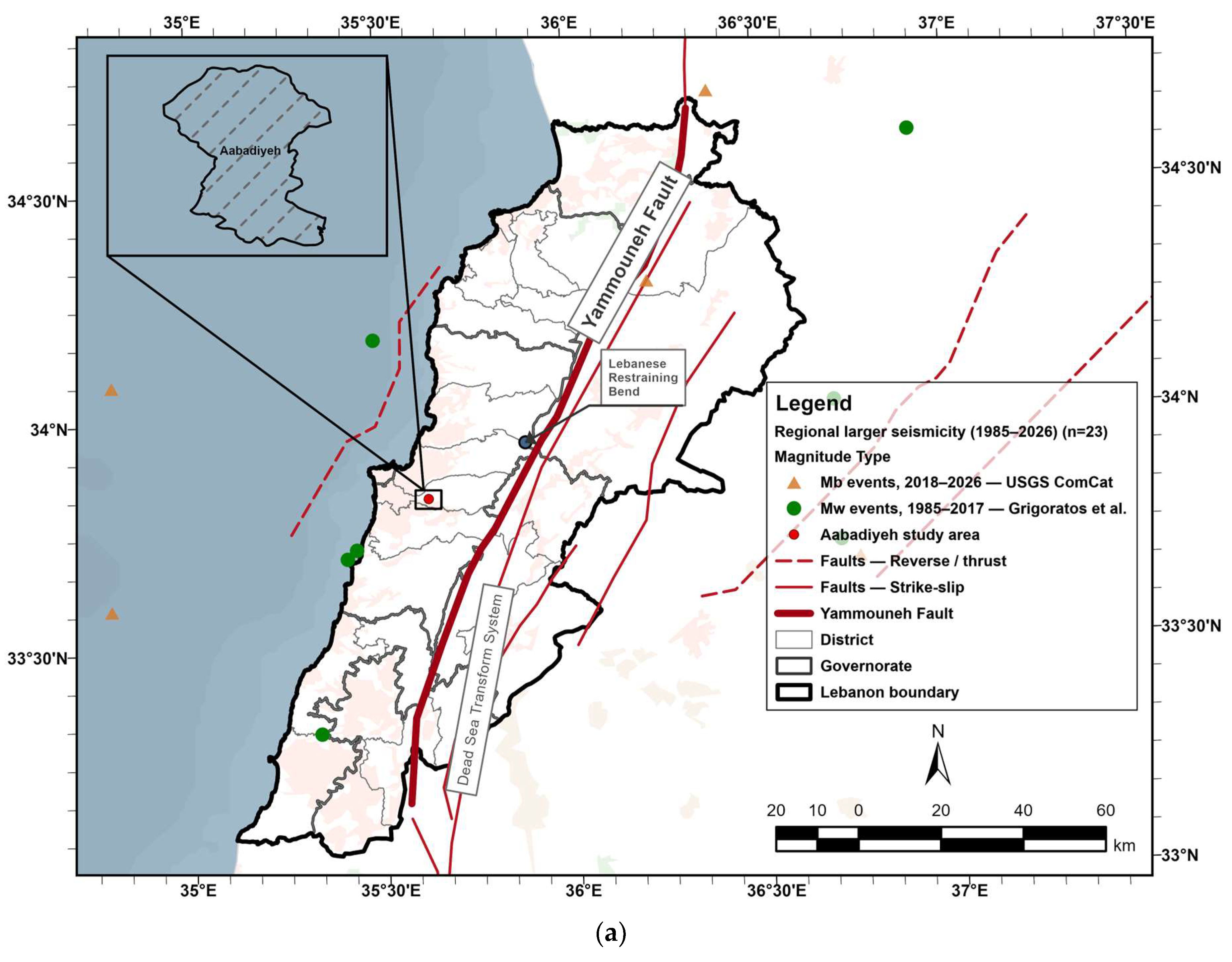
Figure 1. (a) Study area and regional seismicity: (a) location of Aabadiyeh Municipality, Lebanon, within the regional seismotectonic setting, relative to the principal active fault system; (b) magnitude through time for the 23 selected regional events [24,25,26,27]; (c) annual counts for the same event set.
Ijgi 15 00425 g001aIjgi 15 00425 g001bIjgi 15 00425 g001c
Figure 2. EGS workflow and admission logic. Arrows indicate the order of assessment: each candidate layer is assessed at all four gates (G1–G4), a failure at one gate does not stop assessment at the others, and the combined gate outcomes determine one of four dispositions for the stated use (Table 3).
Ijgi 15 00425 g002
Figure 3. (a) Construction-epoch proxy classes in road-network context: 455 buildings post-2000 (class 1), 697 in 1990–2000 (class 2), and 400 pre-1990 (class 3). (b) Spatial distribution of the construction-epoch validation frame and stratified sample.
Ijgi 15 00425 g003
Figure 4. Soil classification schemes derived from the CNRS polygons: (a) building-level two-class criterion, transferred to footprints through the project’s 10 m raster workflow; (b) source-side three-class field on the common grid.
Ijgi 15 00425 g004
Figure 5. Independent two-interpreter validation of the construction-epoch proxy: (a,c) binary confusion matrices for the decision-relevant 1990-or-later versus pre-1990 split, for Interpreters A and B respectively; (b,d) the corresponding three-class matrices for post-2000, 1990–2000, and pre-1990. Rows contain interpreter reference classifications and columns contain GAIA-derived proxy classes.
Ijgi 15 00425 g005
Figure 6. Soil evidence and evidence-gate outcomes for the building-level criterion and the source-side field: (a) recovered two-class building criterion; (b) source-side three-class distribution among matched footprints; (c) gate outcome for the building-level criterion.
Ijgi 15 00425 g006
Figure 7. Spatial distribution of the buildings classified as exploratory High by the ASI.
Ijgi 15 00425 g007
Figure 8. Sensitivity and stability of the exploratory ASI across seven tested construction-epoch weights: (a) high-priority count by age weight; the dashed vertical line marks the historical baseline weight of 0.625 used in Equation (2); (b) cross-scenario class stability.
Ijgi 15 00425 g008
Figure 9. Factor-of-safety and Newmark evidence-gate diagnostics: (a) the 240 tested factor-of-safety reconstruction configurations, plotted by correlation and 99th-percentile relative error, with the retained configuration highlighted (the blue points represent the tested factor-of-safety reconstruction configurations, whereas the orange point identifies the retained configuration selected on the basis of minimum RMSE and MAE); (b) critical-acceleration applicability classes for the non-flat project cells; (c) composition of the project 30 cm displacement class.
Ijgi 15 00425 g009
Figure 10. Composition of cells flagged by the Newmark displacement raster across the tested displacement thresholds, separating valid in-domain predictions from imposed cap values and below-domain extrapolations.
Ijgi 15 00425 g010
Figure 11. Class distribution of the project-specific raster ERI across 90,146 cells.
Ijgi 15 00425 g011
Figure 12. Raster-to-building transfer and building-domain accounting for the historical raster workflow.
Ijgi 15 00425 g012
Figure 13. Consequences of evidence admission for the municipal follow-up queue: (a) exploratory ASI High set versus the retained age-only construction-epoch queue; (b) evidential status of the Newmark 30 cm cells; (c) raster-to-building transfer accounting.
Ijgi 15 00425 g013
Figure 14. Conditionally admitted 400-building preliminary follow-up queue shown in road-network context. The mapped buildings are the pre-1990 construction-epoch class retained for low-consequence municipal triage and subsequent record review, field inspection, and engineering assessment. The queue is a prioritization aid only; it does not represent structural vulnerability, expected damage, code compliance, life-safety risk, or building-specific seismic performance.
Ijgi 15 00425 g014
Table 1. Principal products, spatial support, and role in the audit.
Dataset or ProductSource Support and ProvenanceOriginal SourceTarget Support or RoleProduct DesignationVerification Status
Municipal building inventoryPolygon footprintsMicrosoft Global ML Building Footprints (2023 release) [28], supplemented by manual digitization from Esri World Imagery (2025) [29]1552 decision unitsScreening, zonal transfer, and omission auditCount and source identifiers verified; geometry redistribution remains subject to data-owner permission
GAIA Version 2024 annual impervious area [30,31]30 m Landsat-derived raster, 1985–2024Global Artificial Impervious Area (GAIA), Version 2024Building footprints (modal class per footprint)Construction-epoch proxy from the 1985, 1990, and 2000 annual layersProduct DOI/version and rule verified; original cloud task IDs and export-time environment were not retained
Detailed Lebanese soil map [32]1:50,000 polygonsNational Council for Scientific Research (CNRS) Center for Remote Sensing detailed soil map of LebanonBuilding-level soil criterion and source-side soil fieldSoil_Risk and Seismic_Risk productsEdition and field lineage documented; source geometry is restricted from redistribution
HWSD version 2.0 [33]~1 km (30 arc-second) raster with soil-mapping-unit attribute tablesHarmonized World Soil Database version 2.0 (HWSD2)Attribute lookup through HWSD2_SMU_ID0–20 cm texture and bulk-density proxiesVersion, join key, dominant-layer fields, and fallback rule documented
Digital elevation modelDerived 10 m project rasterDirectorate of Geographic Affairs (DGA) 10 m-interval contours converted to a TIN, rasterized at 10 m, and hydrologically filledTerrain and common model gridElevation, slope, snap, extent, and maskGrid geometry and DEM processing recovered; original contour redistribution remains restricted
Factor-of-safety rasterDerived 10 m project rasterDEM slope, soil/HWSD proxies, TWI-based ru, and the intended infinite-slope relation (Equation (A1)) [32,33,34]Newmark input on the common project gridRaw and post-processed factor of safetyIntended generator documented; no executable lineage/checksum proves that it generated the stored raw surface
Critical-acceleration rasterDerived 10 m project rasterFactor of safety and DEM slope combined using Equation (A2) [35,36]Newmark input and calibration-domain auditApplicability classification and displacement inputEquation and stored output audited; provenance inherits the unresolved raw factor-of-safety input
Newmark displacement rasterDerived 10 m project rasterArias intensity and critical acceleration combined using Supplementary Equation (S4) [37,38,39,40]Threshold and signal auditProject co-seismic displacement implementationFormula and thresholds audited; rejected for operational use because the provenance, applicability, and input-support gates failed independently of threshold choice, and the signal gate failed at the 30 cm decision class
Arias intensity raster (Ia)Derived 10 m project rasterIa_M75 computed from Supplementary Equations (S2) and (S3) using the Travasarou-type Arias-intensity model [40] for a deterministic Mw 7.5 strike-slip rupture on the Yammouneh Fault, with cell-specific rupture distance and site-category indicator terms (Sc, SdS) derived from spatial time-averaged shear-wave velocity in the upper 30 m (VS30) values. Newmark displacement inputScenario-based Arias intensity for the Newmark processing chainScenario, equations, coefficients, spatial inputs, and centroid quality-control calculation documented; computational method verified, but not independently validated against observed shaking
Peak ground acceleration (PGA) rasterDerived 10 m project rasterGEM Global Seismic Hazard Map v2023.1 probabilistic PGA [41,42] (475-year return period, reference rock), used as the ERI PGA component; nearest-neighbor resample to 10 m, then three ordinal classes at 0.360 g and 0.373 gReclassified ERI input on the project gridHistorical three-class shaking componentStored component and ERI contribution verified; source, scenario, and class breaks documented (GEM v2023.1 probabilistic PGA, 475-year, reference rock); audited as a probabilistic input combined with the deterministic Newmark processing chain in the ERI
Slope-risk rasterArchived 10 m project rasterProject slope-risk classification on the common project grid; the generating operation is not documented in the archiveReclassified ERI input on the project gridHistorical two-class slope-risk componentStored component and ERI contribution verified; the class definition was not retrieved from the project archive, so the slope values separating class 1 from class 2 remain undocumented
Source-side soil field (Seismic_Risk)Derived 10 m project rasterThree-class lookup from the CNRS soil polygons (Anthrosols, Cambisols, Luvisols; Arenosols, Leptosols, Regosols; Gleysols), rasterized to the common gridReclassified ERI input on the project gridHistorical three-class soil componentLookup and rasterization documented and class counts reproduce; the polygon-matching residual and the rationale for the two-class reduction were not retrieved from the project archive
Exploratory Age-Soil Index (ASI)Individual building footprints (n = 1552)Weighted combination of construction-epoch and building-level soil codes using Equation (2)Exploratory building-level ASI used for relative municipal triage and sensitivity analysis; not a grid raster, measured hazard variable, or operationally admitted fusion productExploratory ASIFormula reproduced from stored components; retained for exploratory counterfactual only, inheriting the soil layer’s applicability and support limitations
ERIDerived 10 m composite rasterWeighted Sum combination of reclassified Newmark, PGA, slope-risk, and source-side soil rasters using Equation (3)Five-class composite rasterHistorical earthquake-risk-index surfaceFormula reproduced from stored components; end-to-end component lineage remains incomplete
Table 2. EGS gate definitions and evidence requirements.
GateQuestionEvidence ExaminedDecision Implication
G1 Computational provenanceCan the output be reproduced from documented inputs, operations, masks, transfer rules, and parameters?Source identity, code or model records, intermediate outputs, grid definition, deterministic comparison, with declared tolerance only for documented stochastic or approximate proceduresFail (hard failure); a deterministic operational product whose generating chain cannot be recovered is rejected for operational use
G2 ApplicabilityIs the evidence used within its purpose, scale, support, analytical unit, calibration range, and decision context?Source purpose, stated use, source–target support, domain limits, transfer completenessFail when the mismatch is material; the layer is rejected for the declared use; bounded mismatches may receive a conditional pass
G3 Signal validityDoes the decision-relevant class contain meaningful discriminatory information?Occupied classes, thresholds, cap values, placeholders, extrapolations, domain statusPass, pass as numerical variation, threshold-dependent, limited, or numerical variation present but not sufficient status; fail if the operational class contains no valid signal; pass as numerical variation, or numerical variation present but not sufficient status; fail if the operational class contains no valid signal
G4 Input supportAre data, proxy meanings, assumptions, classes, parameters, and weights independently supported?Local observations, reference labels, standards, primary literature, calibration or validationConditional pass only when support is bounded and adequate for a low-consequence purpose; otherwise fail
Table 3. EGS gate status and overall disposition.
GateStatusDefinition
G1 Computational provenancePassThe generating chain is recoverable and the stored output reproduces at every level examined.
Formula passThe documented expression recalculates from the stored components, but a component or its input chain cannot be verified.
Partial provenanceThe documented rule reproduces the stored output, but one or more steps in the generating chain are absent from the archive. Neither a pass, because the unrecorded steps cannot be audited, nor a hard failure, because the principal operation is recoverable and reproduces.
Fail (hard failure)The generating chain of a deterministic product cannot be recovered from the documented record.
G2 ApplicabilityPassThe evidence matches the declared use.
Conditional passThe mismatch between the evidence and the declared use is bounded and not material.
FailThe mismatch between the evidence and the declared use is material.
G3 Signal validityPassThe decision-relevant class carries meaningful discriminatory information.
Pass as numerical variationOrdered variation is present at the decision unit, without an absolute physical interpretation.
Threshold-dependentThe decision-relevant class is discriminatory at some thresholds but not at others.
LimitedThe decision-relevant class separates few decision units from the rest.
Numerical variation present but not sufficientVariation is present, but it does not reproduce the distinctions the declared use requires.
FailThe operational class carries no valid signal.
G4 Input supportPassIndependent support is adequate for the declared use.
Conditional passIndependent support for the declared use is bounded and adequate for a low-consequence purpose.
FailIndependent support is absent or inadequate for the declared use.
Any gateFail by inheritanceA composite fails any gate its components fail for the declared use, regardless of whether its formula reproduces.
Overall dispositionAdmitThe layer enters the retained operational screen. Requires an unconditional pass at all four gates.
Conditionally admitThe layer is permitted only for the specified low-consequence use, with the recorded limitation. Requires a full G1 pass, a bounded and non-material G2 mismatch, a meaningful G3 signal, and bounded G4 support adequate for that purpose.
RejectMapping and discussion for forensic diagnosis are permitted, but the layer is excluded from the retained operational screen. Follows from a hard failure at any single gate; passes at the remaining gates cannot offset it.
Exploratory onlyA composite reproduces at formula level but inherits a failure from a controlling component.
Table 4. Construction-epoch distribution.
ClassCountPercentage of 1552 Buildings
Post-200045529.32%
1990–200069744.91%
Pre-199040025.77%
Total1552100.00%
Table 5. Counts for the two soil products.
ProductClass CountsDenominatorInterpretation
Building-level soil criterion260 class 1; 1292 class 21552Recovered building criterion
Source-side soil field292 class 1; 763 class 2; 495 class 31550 matchedSeparate source-side pedological/raster field
Source-side unmatched21552 total footprintsNo source–polygon match
Table 6. Exploratory ASI sensitivity.
Age WeightSoil WeightLowModerateHighRecords Differing from Baseline
0.500.505846653030
0.550.455846653030
0.600.405846653030
0.6250.3755846653030
0.650.355846653030
0.700.30455697400226
0.750.25455697400226
Table 7. Building-level calibration-domain support.
Domain-Support ClassCountPercentage of 1243 Evaluable BuildingsPercentage of All 1552 Buildings
Entirely in domain45836.85%29.51%
Partly in domain1118.93%7.15%
No in-domain area67454.22%43.43%
Evaluable total1243100.00%80.09%
Table 8. Final EGS gate matrix and operational decisions.
Candidate ProductG1G2G3G4Overall DecisionOperational Consequence
Construction-epoch proxyPassConditional passPassConditional passConditionally admitStandalone low-consequence triage only
Building-level soil criterionPassFailLimitedFailRejectExcluded from retained screen
Source-side soil fieldPartial provenanceFailLimitedFailRejectDescriptive/audit use only
Exploratory ASIFormula passFail by inheritancePass as numerical variationFail by inheritanceExploratory onlyCounterfactual comparison only
Newmark displacement rasterFail at raw-generator levelFailThreshold-dependent; fail at 30 cmFail/insufficientRejectNo operational threshold class retained
ERIFormula pass; component/input-chain failureFail by inheritanceNumerical variation present but not sufficientFail by inheritanceRejectHistorical audited product only
Table 9. External reference-case gate matrix: independent assessor outcomes for the four external products.
External ProductAssessorG1G2G3G4Overall Decision
GAIA (Case 1)Assessor APassConditional passLimitedConditional passConditionally admit
Assessor BPassConditional passLimitedConditional passConditionally admit
SoilGrids (Case 2)Assessor AFailFailNumerical variation present but not sufficientFailReject
Assessor BFailFailLimitedFailReject
Landslide susceptibility (Case 3)Assessor APassConditional passThreshold-dependentConditional passConditionally admit
Assessor BPassConditional passLimitedConditional passConditionally admit
INFORM Lebanon (Case 4)Assessor APassFailPass as numerical variationFailReject
Assessor BPassFailPass as numerical variationConditional passReject
Disclaimer/Publisher’s Note: The statements, opinions and data contained in all publications are solely those of the individual author(s) and contributor(s) and not of MDPI and/or the editor(s). MDPI and/or the editor(s) disclaim responsibility for any injury to people or property resulting from any ideas, methods, instructions or products referred to in the content.