Spatial Dependence and Urban Facility Context of Public Library Use Intensity: Evidence from Seven Metropolitan Cities in South Korea

Abstract

This study examined public library use intensity across seven metropolitan cities in South Korea, considering spatial dependence and the surrounding urban environment. From 485 public libraries, model-specific analytical samples were constructed for visits per m², loans per m², and borrowers per m². Urban facility variables within 1- and 2-km catchments were used as predictors, and academy density was corrected using education office records geocoded using the Kakao Local API. Moran’s I and Anselin–Florax Lagrange Multiplier diagnostics were used to assess spatial dependence among libraries and compare ordinary least squares, spatial autoregressive (SAR), and spatial error model results. Moran’s I indicated significant spatial clustering across all three outcome variables. SAR results revealed that the indirect component accounted for 46.3% and 40.8% of the total academy effect on visits and loans per m², respectively, representing model-based indirect effects rather than direct evidence of user movement. A supplementary negative binomial model using library floor area as an exposure did not corroborate the academy-density association, indicating that this finding is specific to the area-normalized model rather than scale-invariant. These findings highlight the importance of considering spatial dependence and urban facility contexts when interpreting public library use intensity at the regional scale.

1. Introduction

Public libraries are essential facilities that support residents’ access to information while promoting learning and cultural activities. Library use is influenced not only by internal facility characteristics, such as collection size, programs, operating hours, and building size, but also by the surrounding population structure, land use, transportation accessibility, and distribution of educational and commercial facilities [1,2,3,4,5,6]. In metropolitan areas, libraries do not function as isolated facilities; they are embedded within spatially connected usage environments shaped by nearby libraries, educational facilities, and commercial and transportation hubs [7,8,9,10].

Previous studies on public library use primarily employed regression models to examine the relationships between library use and explanatory variables measured at the individual library scale [1,2,3,6]. However, when library use indicators exhibit spatial clustering, conventional regression models that assume independent observations may not adequately account for spatial dependence [11,12,13]. Moreover, simple measures, such as the number of visitors or loans, do not account for differences in library size. A more suitable method would be to examine library use intensity normalized by facility floor area [6]. This study addresses the aforementioned gaps in the literature by considering three variables: visits, loans, and borrowers per m², thereby presenting a detailed analysis of public library use intensity while exploring the spatial dependence and urban facility context of 485 libraries across 7 metropolitan cities in South Korea.

This study explores three objectives. First, it assesses the spatial autocorrelation in public library use intensity across seven metropolitan cities in South Korea. Second, after controlling for city fixed effects, it examines the associations among surrounding urban facility variables and library use intensity by comparing ordinary least squares (OLS), spatial autoregressive (SAR), and spatial error model (SEM) specifications. Third, it uses geographically weighted regression (GWR) to explore local spatial heterogeneity that may be averaged in global models. GWR was employed as an exploratory local heterogeneity analysis to supplement the interpretation of spatial patterns, rather than being used as primary evidence for causal inference.

This study makes three contributions to empirical literature on public library use. First, it applies an established sequence of spatial econometric diagnostics (Moran’s I and Lagrange Multiplier (LM) tests, comparison of OLS, SAR, and SEM specifications, SAR impact decomposition, and exploratory GWR) to public library use intensity in South Korea, a context in which these diagnostics have rarely been applied together. Second, it demonstrates that academy variables derived from OpenStreetMap may undercount officially registered academies, and constructs an improved measure by combining education office records with Kakao geocoding. Third, it quantifies the model-based indirect effect component through SAR impact decomposition, capturing spatially structured associations that are difficult to identify in facility-level analysis, while explicitly avoiding the interpretation of these indirect effects as direct evidence of actual user movement between libraries.

2. Literature Review and Theoretical Background

2.1. Determinants of Public Library Use: Achievements and Methodological Limits

Previous studies analyzed public library use based on a wide range of factors, including population size, age structure, educational attainment, income, library collections, program provisions, and facility accessibility [1,2,3,4,5,6]. Studies at the facility level primarily focused on the relationships between internal library resources and performance indicators, while regional-level studies focused on socioeconomic demands and accessibility of libraries [1,2,3,4,5]. Koontz et al. [14] proposed neighborhood-based in-library use performance measures to capture disparities in use patterns that system-wide aggregation can obscure. Recent studies adopted the floating catchment area (FCA) approach to determine library accessibility with greater precision. Larimore et al. [15] analyzed the spatial inequalities in library accessibility in Calhoun County in the United States of America, using the enhanced two-step FCA method. Furthermore, Dunne et al. [16] evaluated the effects of administrative boundary reorganization on library accessibility in Pembrokeshire, United Kingdom. Complementary approaches include a scalable method for assessing the spatial equity of library locations across socioeconomic subgroups [17] and an analysis of regional variation in population-weighted distance to public libraries across the United States [18]. Koo and Chang [19] applied spatial regression methods, conceptually similar to those used in the present study, to examine the accessibility of public libraries in Busan, one of the seven metropolitan cities considered here. However, these studies primarily focused on accessibility and did not model the spatial dependence of library use intensity. Consequently, approaches that treat individual libraries as independent observations may not adequately capture the influence of neighboring environments or the network effects among libraries.

2.2. Urban Facility Environment, Point of Interest (POI) Data, and Public Facility Use

Public libraries are embedded within everyday activity spaces near educational, cultural, commercial, and transportation facilities. The density of academies, cafés, cinemas, subway stations, and bus stops can serve as proxies for pedestrian activity, opportunities for prolonged stay, educational demand, and urban centrality [7,8,9,20,21]. However, POI data may vary in completeness and classification depending on the data source. In particular, facilities that are administratively registered, such as private academies, may exhibit substantial discrepancies between official records and commercial or open-source POI datasets [6,8,20]. Therefore, when urban facility variables are used in empirical analysis, the data sources and procedures used for data correction should be clearly documented.

2.3. Spatial Econometric Methods Applied to Urban Public Facility Demand

Moran’s I is a widely used statistic for diagnosing spatial autocorrelation between either dependent variables or model residuals [13]. When spatial autocorrelation is present, OLS alone may not adequately account for spatial dependence. In such cases, Anselin–Florax LM diagnostics can be used to assess whether SAR or SEM specifications are warranted [11,12]. The SAR model incorporates the values of neighboring observations through a spatial lag of the dependent variable; the impact decomposition proposed by LeSage and Pace [22] can be used to estimate the direct and indirect effects. The indirect effects represent statistical quantities derived from the model and spatial weights matrix rather than denoting direct evidence of actual user movement. The GWR model relaxes the assumption of spatially constant coefficients in global models and enables the exploration of spatial variations in local parameter estimates [23]. For public facility use, where urban structure and usage patterns vary across regions, global average coefficients alone may not be adequate to explain local differences [10,24]. Spatially explicit modeling of library circulation itself predates contemporary spatial econometric diagnostics: Ottensmann [25] applied gravity-model spatial-interaction principles to predict circulation in a public library system, illustrating a long-standing interest in spatially structured models of library use. In the current study, GWR was not used as an alternative to the SAR model but as supplementary analysis to examine the local heterogeneity underlying the global model results.

2.4. Research Gap

The literature review conducted in the current study revealed several important gaps.

Table 1. Comparison between previous research and the present study.

Research Stream	Current Approach	Remaining Limitation	Present Study	References
Library use determinants	Explaining use based on facility- and regional-level variables	Spatial dependence not explicitly examined	Moran’s I, LM diagnostics, and SAR–SEM comparison	[1,2,3,4,5,6]
Accessibility and GIS	Distance- and catchment-based FCA measures	Limited interpretation of spatial spillover effects	Use intensity + SAR impact decomposition	[4,5,9,6,22,15,16]
Urban POI data	Use of POI density as a proxy for urban environments	Inconsistencies across data sources	Official records + Kakao geocoding	[7,8,9,20,21]
Spatial econometrics for public services	Spatial lag and spatial error models	Limited application to public libraries	Selection of the optimal model for each indicator of library use intensity	[11,12,26,27,28,13,29,22]
Local coefficient analysis	Exploration of regional variation using GWR	Risk of overinterpreting local coefficients as causal effects	Restricted to exploratory analysis	[23,24,10]

Abbreviations: geographic information system (GIS), Lagrange multiplier (LM), spatial autoregressive model (SAR), spatial error model (SEM), floating catchment area (FCA), point of interest (POI), geographically weighted regression (GWR).

systematically summarizes these gaps.

3. Materials and Methods

3.1. Study Area and Data Sources

In this study, we considered the data of public libraries located across seven metropolitan cities in South Korea, namely, Seoul, Busan, Daegu, Incheon, Gwangju, Daejeon, and Ulsan. The original dataset included 485 public libraries; the final analytical samples for each outcome variable comprised libraries with valid use and gross floor area data required for the corresponding analysis. Figure 1 illustrates the spatial distribution of the libraries and the geographic extent of the seven metropolitan cities considered in this study.

3.2. Outcome Variables and Sample Refinement

The outcome variables considered in this study included visits, loans, and borrowers per m²; the corresponding indicators were calculated by dividing the annual number of visits, loans, and borrowers by the library’s gross floor area, respectively. These area-normalized indicators were used to mitigate the advantage of larger libraries in terms of absolute use volume and to facilitate comparisons of use intensity relative to facility size [6]. However, as the gross floor area did not distinguish among service, shared, and administrative spaces, it did not fully represent the demand relative to the area actually available for library users. This limitation is discussed separately in Section 5.7 (Limitations).

The sample refinement process for the final analytical datasets is summarized in

Table 2. Sample refinement process adopted in this study.

Outcome Variable	Original Dataset (n)	Excluded Because of Missing or Invalid Gross Floor Area or the Lack of Outcome-Related Data	Additional Exclusions Because of Missing Use Data or the Lack of Derived Outcome Values	Final Analytical Sample (n)
Visits per m2	485	132	18	335
Loans per m2	485	132	33	320
Borrowers per m2	485	132	33	320

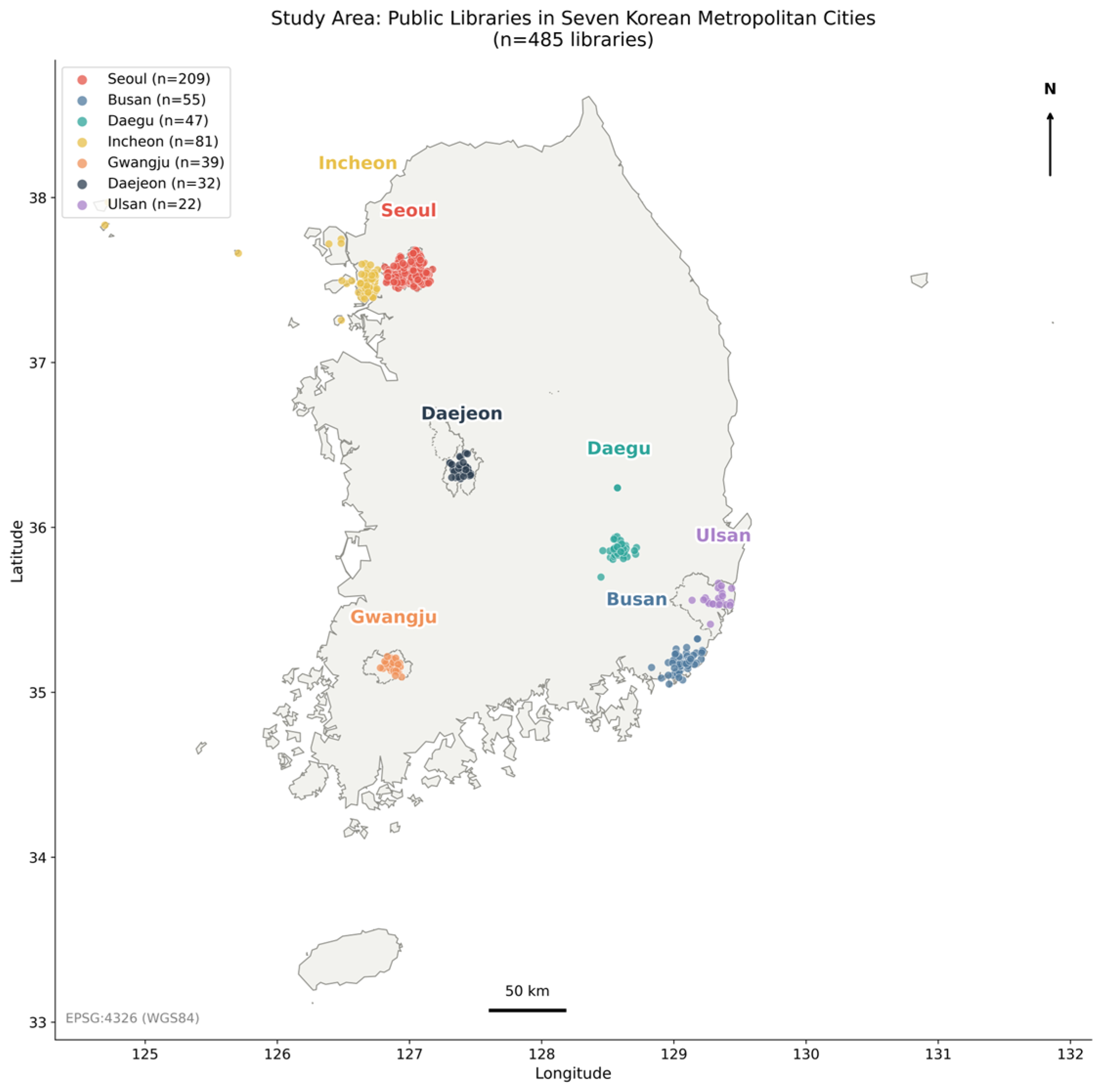
Note: Sample sizes (n) were calculated from the final analytical datasets. The additional exclusion category was determined based on observations with missing derived outcome variables for each respective outcome.

. From the 485 libraries in the original dataset, 132 were excluded because of missing or invalid data on gross floor area and outcome-related use data. An additional 18 libraries were excluded from the “visits per m²” analysis because of missing derived outcome values; furthermore, 33 additional libraries were excluded from the analyses of loans and borrowers per m² because of missing use data or the lack of derived outcome values. Thus, the final analytical samples comprised 335 libraries for visits per m² and 320 libraries for each of loans and borrowers per m².

3.3. Analytical Framework and Model Specification

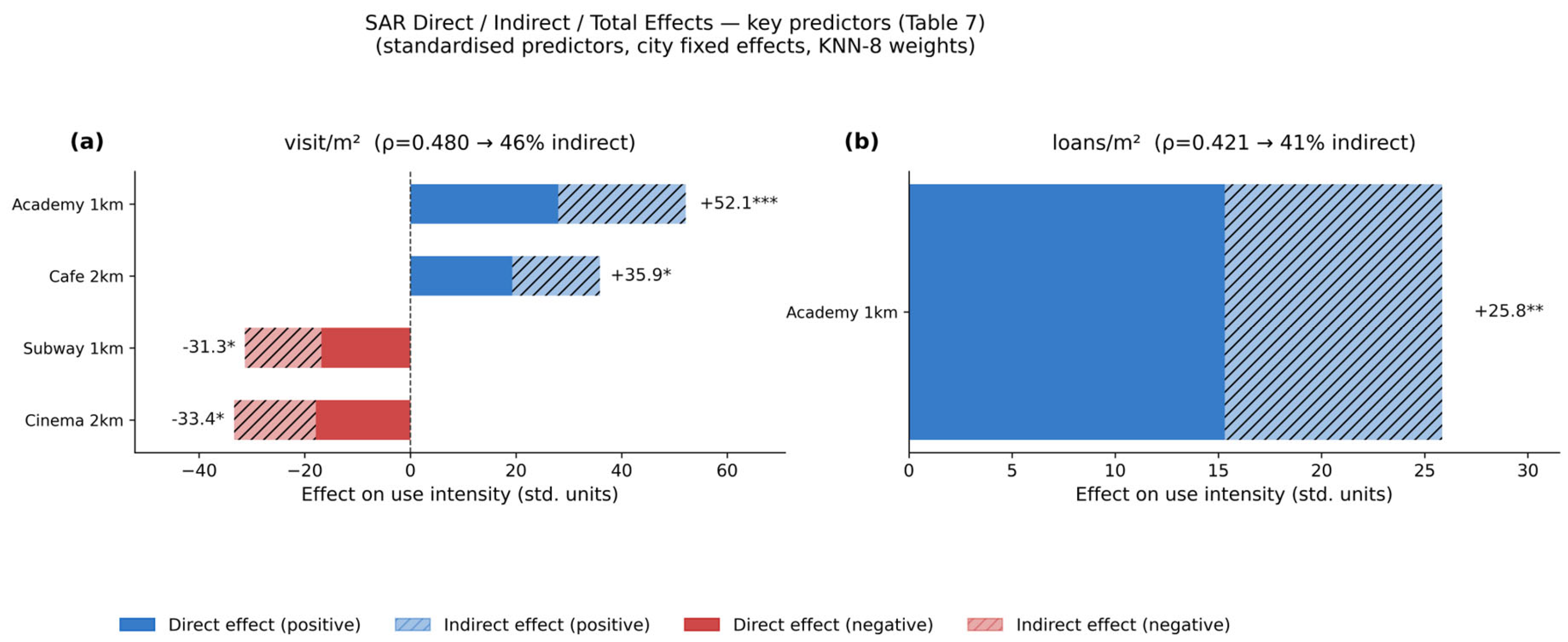
The predictor variables comprised the number of urban facilities located within 1- and 2-km catchments surrounding each library. Candidate variables included academies, cafés, cinemas, subway stations, bus stops, parks, schools (elementary, middle, and high schools), and supermarkets. The final models for each outcome variable included a subset of these catchment-specific variables based on diagnostic results and the variable selection procedure.

The candidate predictor set was narrowed once, before estimating any of the reported models, based on two preliminary diagnostics: severe multicollinearity between the 1- and 2-km versions of school-count variables (variance inflation factor [VIF] as high as 84 for elementary schools at 2 km), and weak or inconsistent agreement between independently sourced computations of the park and 2-km bus-stop variables. Elementary, middle, and high schools and parks were accordingly retained at 1 km only, while cafés, cinemas, supermarkets, subway stations, bus stops, and academies retained both 1- and 2-km versions. This resulting 17-variable candidate set, together with city fixed effects, was then applied identically to all three outcome variables (visits, loans, and borrowers per m²) and all three model families (OLS, SAR, and SEM); no further outcome-specific variable elimination occurred at the estimation stage.

The rationale for selecting each predictor is as follows. Academies represent major destinations for students and parents engaged in recurring education-related travel and may therefore generate usage patterns that complement those of nearby public libraries [20]. Cafés were included as proxies for complementary use because, according to Ray Oldenburg’s Third Place theory [21], they function as venues for leisure, learning, and extended stays within individuals’ routine activity spaces in ways similar to public libraries. Cinemas were included as potentially competing leisure facilities that may substitute for library use during discretionary leisure time. Subway stations and bus stops were included as indicators of public transportation accessibility, reflecting high-density commercial characteristics typically associated with transportation hubs. Consequently, the direction of their associations with library use was expected to be ambiguous. Parks, schools, and supermarkets were included as background variables to control for the general density of public, educational, and commercial facilities within the surrounding urban environment. Variables representing 1- and 2-km catchments for the same facility type were initially constructed to distinguish between walkable neighborhoods and broader activity areas.

The academy variable was constructed using education office records of registered private academies. The addresses in the official dataset were geocoded using the Kakao Local API, and the resulting coordinates were used to calculate the number of officially registered academies within 1- and 2-km catchments of each library.

The reference dates of the datasets were not completely aligned. The library use statistics represented the annual usage for 2024, while the official bus-stop dataset corresponded to the version dated 31 October 2025. Kakao geocoding was performed on 8 June 2026. Accordingly, the urban facility variables should be interpreted as cross-sectional proxies for the recent urban environment and not as exposure measures that correspond exactly to the same year as the library use statistics for 2024.

Socioeconomic variables, such as population, income, and age structure, were not included in the final models. Rather than estimating a causal model that fully controlled for demographic and socioeconomic characteristics, the present study focuses on exploring the spatial associations between urban facility POI variables and public library use intensity. Although city fixed effects were included to account for average differences across metropolitan cities, the socioeconomic heterogeneity within the cities was not fully controlled. Therefore, the estimated relationships should be interpreted as conditional associations rather than as independent causal effects of urban facility variables. This issue is discussed further in Section 5.7.

Table 3. Primary data sources and final datasets used in this study.

Data	Final Dataset	Purpose	Reference Date/Status
Final library analytical dataset	Model-ready library-level dataset	Outcome variables, urban facility variables, and city fixed effects	Library use statistics for 2024
Official academy records	Official academy administrative source	Source addresses for registered academies	Public administrative records available at the time of data collection
Kakao geocoding output	Cleaned Kakao-geocoded address dataset	Geocoded academy locations	Geocoding version 2026-06-08
Library-level academy counts	Library-level academy buffer counts	Construction of academy variables within 1 and 2 km catchments	Based on Kakao-geocoded records
VIF diagnostics	Supplementary Table S1	Assessment of multicollinearity	Final analytical dataset
K sensitivity analysis	Supplementary Table S2	Sensitivity analysis of the spatial weights matrix	KNN 5,6,8,10

Abbreviations: Variance inflation factor (VIF), K-nearest neighbors (KNN).

presents the data sources and final datasets used in this study.

3.4. Analytical Procedure

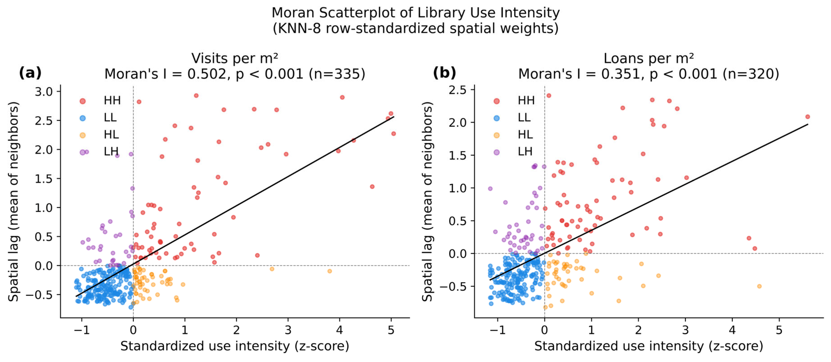
The analytical procedure comprised several sequential steps. First, the analytical sample was determined for each outcome variable. Next, spatial autocorrelation was assessed using Moran’s I computed from the observed outcome values. An OLS model with city fixed effects was then estimated, and Moran’s I tests were conducted on the residuals. Subsequently, Anselin–Florax and robust LM diagnostics were applied, followed by comparisons of the OLS, SAR, and SEM specifications. For outcome variables for which the SAR model was selected, the direct, indirect, and total impacts were estimated. Finally, local spatial heterogeneity was explored using GWR.

• The OLS, SAR, and SEM specifications can be expressed as shown below in Equations (1)–(3), respectively:

y = X β + city fixed effects + ε

(1)

y = ρ W y + X β + city fixed effects + ε

(2)

y = X β + city fixed effects + u, u = λ W u + ε

(3)

In the current study, KNN-8 was used as the primary algorithm. The robustness of this model was evaluated through sensitivity analyses using KNN-5, KNN-6, and KNN-10. The choice of k in a KNN spatial weights matrix has no universally correct value: as Gerkman and Ahlgren [30] note in their review of practices in the applied spatial econometrics literature, “the number k is usually unknown, and must be inferred from the data” (cf. [22], p. 162). It is generally established through sensitivity analysis across a plausible range rather than a fixed rule of thumb, which is the approach followed here. For bus stops within the 2-km catchment, the maximum VIF was 8.88. The VIF values for academy density were 3.11 and 3.72 for the 1- and 2-km catchments, respectively, while those for café density were 3.53 and 4.36, respectively. Although café density was significant in some models, it was not included in the main interpretation because of potential multicollinearity and its role as a general proxy for urban amenities. Neighbor relationships under KNN-8 were computed on unprojected coordinates without imposing city-level constraints. In practice, only 4 of 2680 directed neighbor edges (0.15%) for the visits per m² sample crossed metropolitan city boundaries. Although the resulting spatial weights matrix ensured that each library had eight neighbors, it did not form a single connected graph; instead, it was partitioned into five weakly connected components corresponding to geographically distinct metro-area clusters. As a robustness check, the SAR models for visits and loans per m² were re-estimated under a Voronoi-tessellation rook-contiguity matrix and a 2-km distance-band matrix (projected to EPSG:32652). The academy-density association within 1 km remained positive and significant under both alternative specifications (p ≤ 0.022 in all cases; Table S4). However, the estimated SAR parameter ρ varied across spatial weights matrixes, taking values of 0.48, 0.36, and 0.15 under the KNN-8, Voronoi, and the distance-band specifications, respectively. This pattern is consistent with ρ being scaled by the connectivity density of the spatial weights matrix and therefore does not represent an absolute, specification-invariant quantity.

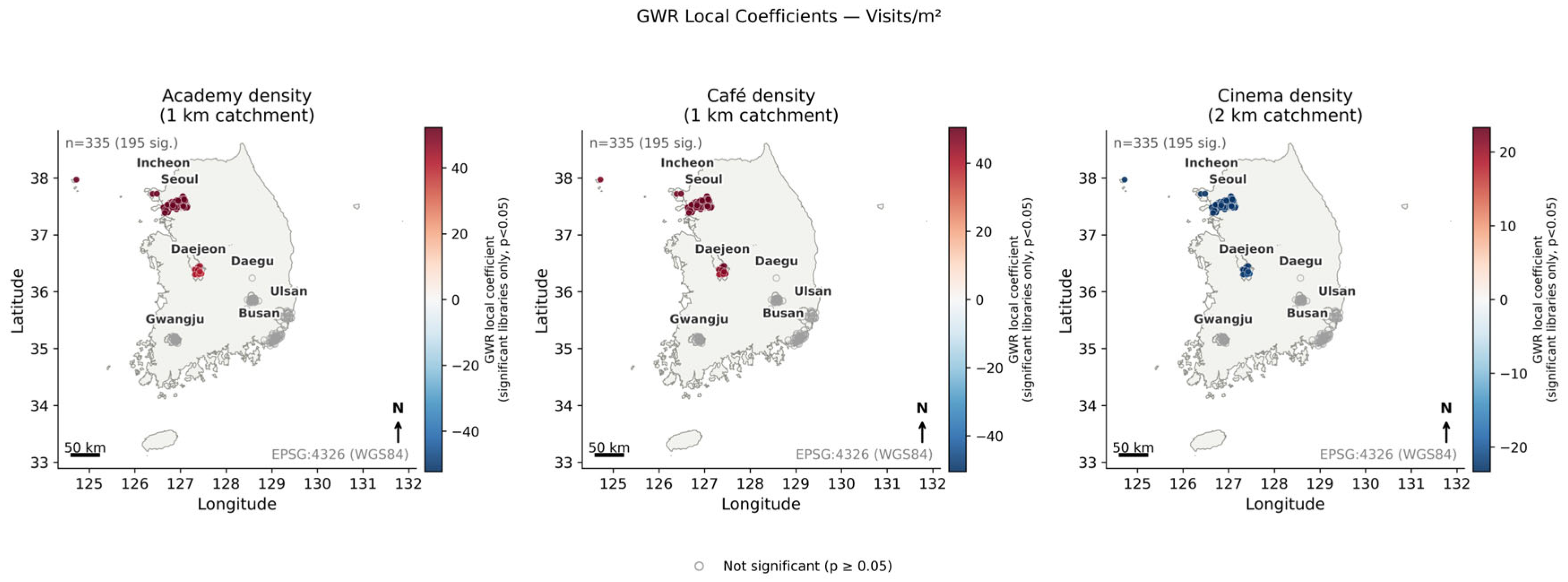
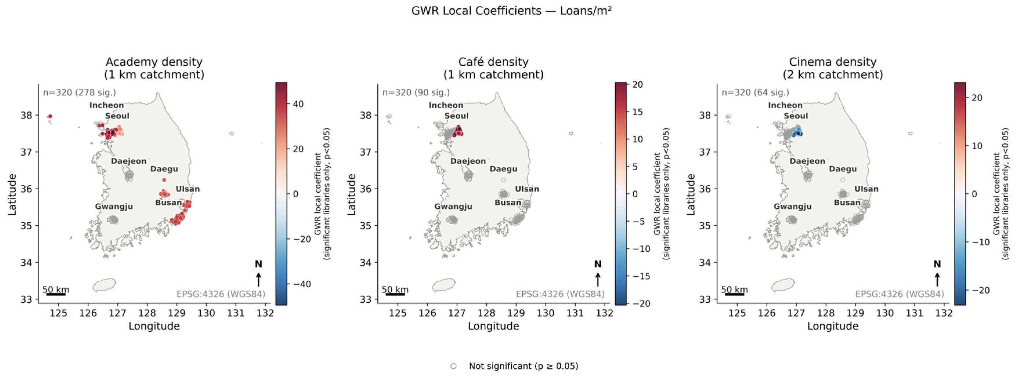
For borrowers per m², the Moran’s I test on the residuals of the OLS model with city fixed effects and the robust LM diagnostic results were both nonsignificant. Accordingly, the final interpretation was based on the OLS model and not an SAR specification. As GWR served a different analytical purpose from SAR, we considered it a separate exploratory analysis. City fixed effects were not included in the GWR models because city dummy variables could absorb most location-based variations captured by local regression or reduce the stability of local design matrixes in cities with relatively small sample sizes. This design choice follows general guidance on GWR specification, which cautions against including spatially clustered categorical or grouping variables in GWR models because of the risk of local multicollinearity in the local design matrixes [31]. Therefore, the GWR results were interpreted as supplementary evidence of spatial heterogeneity rather than being considered as confirmatory results supporting the SAR and OLS models. The GWR models further used a reduced six-variable specification consisting of academy (1 km), café (1 km), cinema (2 km), bus-stop (1 km), subway-station (2 km), and high-school (1 km) densities, rather than the full 17-variable SAR/OLS specification. This reduced specification retained one representative predictor from each of the education, culture, transportation, and commerce categories used in our earlier physical-factor study of Busan public libraries [6], thereby preserving degrees of freedom given the local bandwidths (128–266 neighboring observations). However, this set does not precisely reproduce the variable and radius choices of that earlier study. Consequently, GWR and SAR/OLS coefficients differed in both the inclusion of city fixed effects and the predictor set used and should not be compared directly in magnitude.

The statistical significance of Moran’s I was evaluated using 999 permutations. The SAR and SEM models were estimated using maximum likelihood with spreg.ML_Lag and spreg.ML_Error, respectively. The GWR analyses were conducted using the UTM Zone 52N (EPSG:32652) projected coordinate system, an adaptive bisquare kernel, and bandwidth selection based on the corrected Akaike Information Criterion (AICc). The analytical environment comprised Python 3.13.9 with libpysal 4.14.1, esda 2.9.0, spreg 1.9.0, and mgwr 2.2.1 (Python Software Foundation, Wilmington, DE, USA).

4. Results

4.1. Spatial Autocorrelation and Model Selection

The Moran’s I values calculated from the observed outcome values were significant for all three outcome variables, with values of 0.502 (p < 0.001) for visits per m², 0.351 (p < 0.001) for loans per m², and 0.167 (p = 0.002) for borrowers per m². After controlling for city fixed effects, Moran’s I tests performed on the OLS residuals remained significant for visits (0.095, p = 0.002) and loans (0.092, p = 0.003) per m², while the residual Moran’s I result for borrowers per m² was nonsignificant (−0.029, p = 0.147).

Table 4. Spatial autocorrelation and Lagrange Multiplier (LM) diagnostics.

Outcome Variable	n	Moran’s I for Observed Values (p)	Moran’s I for OLS Residuals (p)	Robust LM-Lag (p)	Robust LM-Error (p)
Visits per m2	335	0.502 (<0.001)	0.095 (0.002)	50.520 (<0.001)	13.368 (<0.001)
Loans per m2	320	0.351 (<0.001)	0.092 (0.003)	22.525 (<0.001)	6.808 (0.009)
Borrowers per m2	320	0.167 (0.002)	−0.029 (0.147)	1.068 (0.301)	1.928 (0.165)

Note: For borrowers per m², neither Moran’s I for the OLS model residuals nor the robust LM-Lag and robust LM-Error diagnostics were significant. Accordingly, the OLS model with city fixed effects was retained as the final model for interpretation. Abbreviations: Lagrange multiplier (LM), ordinary least squares (OLS).

presents the results for spatial autocorrelation and LM diagnostics conducted in this study. Figure 2 presents the Moran scatterplots for the outcomes of library use intensity.

4.2. Model Fit Comparisons

For visits and loans per m², spatial autocorrelation remained in the OLS residuals, and the robust LM-Lag diagnostic was significant. For these two outcome variables, the SAR model with city fixed effects yielded lower AIC values and substantially reduced residual spatial autocorrelation. In contrast, for borrowers per m², neither the Moran’s I test on the OLS residuals nor the robust LM-Lag (p = 0.301) and LM-Error (p = 0.165) diagnostics were significant. Accordingly, the OLS model with city fixed effects was retained as the final model for interpretation.

Table 5. Comparison of the ordinary least squares (OLS), spatial autoregressive (SAR), and spatial error model (SEM) results employed in this study.

Outcome Variable	Model	n	R2/pR2	AIC	Spatial Parameter	Residual Moran’s I	p
Visits per m2	OLS	335	0.440	3987.870	-	0.095	0.002
Visits per m2	SAR	335	0.516	3950.512	ρ = 0.480	−0.046	0.032
Visits per m2	SEM	335	0.402	3967.238	λ = 0.537	0.239	0.001
Loans per m2	OLS	320	0.299	3605.364	-	0.092	0.003
Loans per m2	SAR	320	0.360	3584.922	ρ = 0.421	−0.015	0.329
Loans per m2	SEM	320	0.274	3588.995	λ = 0.475	0.174	0.001
Borrowers per m2	OLS	320	0.232	2650.056	-	−0.029	0.147
Borrowers per m2	SAR	320	0.233	2651.651	ρ = −0.075	−0.017	0.277
Borrowers per m2	SEM	320	0.231	2648.199	λ = −0.208	−0.036	0.062

Note: The SAR model with city fixed effects was selected as the final model for interpreting visits and loans per m². Although the SEM yielded a slightly lower AIC than that of the OLS model for borrowers per m², neither Moran’s I for the OLS residuals nor the robust LM diagnostics supported the need for a spatial model. Consequently, the final interpretation for borrowers per m² was based on the OLS model with city fixed effects using HC3 robust standard errors. Abbreviations: number of libraries in sample (n), Akaike Information Criterion (AIC).

presents a comparison of the three models considered in this study. For completeness, Table 5 also reports the SEM specification for borrowers per m² (λ = −0.208); this specification was not selected for interpretation, and its residual spatial autocorrelation (Moran’s I = −0.036, p = 0.062) does not reach the conventional 0.05 significance threshold used elsewhere in this study for model selection. Because the decisive diagnostics for this outcome—Moran’s I on the OLS residuals and both robust LM tests—were all clearly nonsignificant, a more complex two-parameter specification such as SARMA was not additionally fitted for borrowers per m²; such a specification may nonetheless be a useful direction for future work on outcomes exhibiting a plausible mixture of positive and negative spatial dependence.

4.3. SAR Estimation Results

In the SAR model for visits per m², academy density within the 1-km catchment was positively associated with library use intensity (β = 27.12, z = 3.49, p < 0.001). Café density within the 2-km catchment was also positively associated with visits per m² (β = 18.67, z = 2.02, p = 0.044). In contrast, cinema density within the 2-km catchment (β = −17.36, p = 0.025) and subway-station density within the 1-km catchment (β = −16.30, p = 0.044) were negatively associated with visits per m².

For loans per m², the SAR model identified academy density within the 1-km catchment as the only variable with a significant positive association (β = 14.97, z = 2.61, p = 0.009). In the OLS model for borrowers per m², academy density within the 2-km catchment (β = 6.13, t = 2.28, p = 0.023) was positively associated with the outcome, whereas bus-stop density within the 2-km catchment showed a negative correlation (β = −5.18, t = −2.13, p = 0.034).

Table 6. Key coefficients from the final models.

Variable	Visits per m2 SAR β(z)	Loans per m2 SAR β(z)	Borrowers per m2 OLS β(t)
Academy density (1 km)	27.12 (3.49) ***	14.97 (2.61) **	−0.22 (−0.15)
Academy density (2 km)	-	-	6.13 (2.28) *
Café density (1 km)	-	-	2.35 (1.31)
Café density (2 km)	18.67 (2.02) *	7.43 (0.99)	-
Cinema density (2 km)	−17.36 (−2.24) *	−5.81 (−0.85)	-
Subway-station density (1 km)	−16.30 (−2.01) *	−1.29 (−0.18)	-
Bus-stop density (2 km)	-	-	−5.18 (−2.13) *

Note: The results for visits and loans per m² are based on the SAR model with city fixed effects. The results for borrowers per m² are based on the OLS model with city fixed effects using HC3 robust standard errors. The dashes (-) indicate a variable that was estimated but not highlighted for that outcome (see Section 3.3). * p < 0.05, ** p < 0.01, *** p < 0.001. Abbreviations: ordinary least squares (OLS), spatial autoregressive model (SAR).

presents the key coefficients from the final models considered in this study.

4.4. Decomposition of SAR Impacts

SAR impact decomposition was performed only for visits and loans per m², as these outcome variables were modeled using SAR specifications. For visits per m², the total effect of academy density within the 1-km catchment was 52.14, comprising a direct effect of 28.01 and an indirect effect of 24.14. The indirect component accounted for 46.3% of the total effect. For loans per m², the total effect of academy density within the 1-km catchment was 25.85, comprising a direct effect of 15.31 and an indirect effect of 10.53. The indirect component represented 40.8% of the total effect (see

Table 7. Spatial autoregressive (SAR) impact decomposition.

Outcome Variable	Variable	Direct Effect	Indirect Effect	Total Effect	Indirect Effect (%)
Visits per m2	Academy density (1 km)	28.01	24.14	52.14	46.3
Visits per m2	Café density (2 km)	19.28	16.62	35.90	46.3
Visits per m2	Cinema density (2 km)	−17.92	−15.45	−33.37	46.3
Visits per m2	Subway-station density (1 km)	−16.83	−14.51	−31.34	46.3
Loans per m2	Academy density (1 km)	15.31	10.53	25.85	40.8

Note: SAR impact decomposition was not performed for borrowers per m² because the final selected model was ordinary least squares (OLS). The identical proportion of indirect effects within each outcome variable is an inherent property of the SAR model, determined by the spatial weights matrix and the estimated spatial autoregressive parameter (ρ).

). Figure 3 presents the direct, indirect, and total impacts estimated from the SAR models for visits and loans per m².

4.5. GWR Results: Spatial Heterogeneity of Predictor Effects

For the GWR model for visits per m², the optimal bandwidth comprised 266 neighboring observations (79% of that outcome’s analytical sample), while that for loans per m² was 128 (40%). The GWR model for visits per m² achieved a global coefficient of determination (R²) of 0.434, AICc of 3980.851, and mean local R² of 0.300; for loans per m², the corresponding values were 0.406, 3588.499, and 0.312, respectively (see

Table 8. Summary of geographically weighted regression (GWR) models.

Outcome Variable	n	Bandwidth	Global R2	AICc	Mean Local R2
Visits per m2	335	266	0.434	3980.851	0.300
Loans per m2	320	128	0.406	3588.499	0.312

Abbreviations: sample size (n), coefficient of determination (R²), corrected Akaike Information Criterion (AICc).

for detailed GWR results).

Table 9. Summary of geographically weighted regression (GWR) local coefficients for academy density within the 1-km catchment by metropolitan city, including the standard deviations of local coefficients within each city.

Outcome Variable	Metropolitan City	n	Mean Coefficient (SD)	Libraries with Significant Positive Coefficients (n)
Visits/m2	Seoul	136	52.21 (0.07)	136
Visits/m2	Incheon	34	52.08 (0.09)	34
Visits/m2	Daejeon	25	42.21 (1.90)	25
Visits/m2	Busan	49	20.77 (0.22)	0
Visits/m2	Daegu	39	20.92 (0.16)	0
Visits/m2	Gwangju	31	11.13 (0.42)	0
Visits/m2	Ulsan	21	21.80 (0.15)	0
Loans/m2	Seoul	137	30.50 (10.91)	137
Loans/m2	Busan	49	35.46 (0.27)	49
Loans/m2	Daegu	35	33.30 (0.15)	35
Loans/m2	Incheon	42	43.92 (2.56)	42
Loans/m2	Ulsan	15	34.22 (0.13)	15
Loans/m2	Gwangju	24	21.62 (0.34)	0
Loans/m2	Daejeon	18	23.36 (4.32)	0

Abbreviations: sample size (n).

presents the GWR local coefficients for academy density (1 km), the focal variable given its consistent significance across cities, including the standard deviations of local coefficients within each city. Corresponding summaries for the other five GWR predictors (café density 1 km, cinema density 2 km, bus-stop density 1 km, subway-station density 2 km, and high-school density 1 km) are reported in Table S3. Figure 4 and Figure 5 show the local GWR coefficients for academy, café, and cinema densities with respect to the visits and loans per m², respectively. These city-level standard deviations describe the dispersion of local point estimates among the individual libraries within each city; they do not represent the standard error of any single local coefficient estimate, and the present data do not support formal statistical tests of whether GWR coefficients differ significantly between cities.

5. Discussion

5.1. Spatial Dependence and Model Selection

Spatial autocorrelation was identified for both visits and loans per m² in the observed values as well as in the residuals of OLS models. The SAR model with city fixed effects reduced the residual spatial autocorrelation more effectively than either the OLS or SEM models. These findings indicate that public library use intensity is not solely an attribute of individual libraries but is embedded within the spatial continuity of neighboring libraries and their surrounding urban environments [11,12,13,22,26,27,28,29]. However, these results provide statistical evidence of spatial dependence rather than presenting direct evidence of user movement between libraries. A small but significant residual autocorrelation remained in the visits per m² SAR residuals (Moran’s I = −0.046, p = 0.032), indicating that the single spatial lag parameter did not fully absorb the spatial dependence in this outcome. This residual pattern was itself sensitive to the choice of spatial weights matrix (larger under a Voronoi-based specification, resolved under a 2-km distance-band specification; see Section 3.4), consistent with the possibility of a mixed positive/negative spatial autocorrelation process that a single ρ parameter cannot fully capture.

For borrowers per m², the Moran’s I values calculated from the observed values were significant, while those for the OLS residuals with city fixed effects were not. This suggests that the number of registered borrowers may be more strongly influenced by city-level fixed effects or institutional characteristics of individual libraries than that of visits or loans. One plausible interpretation is that “borrowers” reflects registered membership status, a more administrative, one-time registration event, rather than a repeated-visit behavior such as visits or loans; therefore, it may be less associated with the spatially contiguous foot-traffic patterns that visits and loans reflect, and more dependent on library-specific institutional factors such as onboarding events or school partnerships. This distinction has empirical support at the national level. Across Korean public libraries, the number of registered borrowers is reported to have decreased by 57.5% between 2015 and 2019 while the number of items loaned increased by 18.2% over the same period, indicating that registration counts and usage-volume counts can move in opposite directions and are not interchangeable measures of library use [32]. This interpretation remains speculative and requires validation using additional data, such as membership-registration event records.

5.2. Academy Density: An Association Specific to the Area-Normalized Specification

The academy variable, constructed from education office records and refined through Kakao geocoding, exhibited significant positive associations with the visits and loans per m² within the 1-km catchment. For borrowers per m², academy density within the 2-km catchment was significantly associated with the outcome. These findings suggest that libraries located in areas with a high concentration of academies are more likely to be situated within neighborhoods characterized by intensive educational and learning activities [6,20,21]. However, as this study is based on cross-sectional data, the results do not imply that academy density results in greater library use. Notably, academy density should be interpreted as a proxy reflecting multiple characteristics of the surrounding urban environment, including educational demand, the mobility patterns of students and parents, mixed residential and commercial land use, and urban centrality. As a further robustness check, we fitted negative binomial models for the raw annual counts of visits, loans, and borrowers, using library floor area as an offset rather than as a normalizing denominator, with the same predictor set and city fixed effects as those in the main models. Under this specification, academy density within 1 km was not significantly associated with any outcome (incidence rate ratio = 1.10, p = 0.22 for visits; 0.94, p = 0.57 for loans; 0.98, p = 0.86 for borrowers), and this null result persisted after accounting for residual spatial autocorrelation in the visits model via Moran eigenvector spatial filtering. Disagreement between these two specifications is consistent with established statistical results on ratio-based outcomes. Constructing a rate or ratio by dividing a dependent variable by a denominator can alter partial regression coefficients, and may even reverse the sign of an association, relative to a specification that treats the same denominator as an offset or covariate. This occurs because the two approaches impose different functional-form and error-variance assumptions on the underlying numerator–denominator relationship [33,34]. We interpret this discrepancy as indicating that the academy-density association is a property of the area-normalized, additive specification that motivates this study’s spatial dependence framework, rather than as a scale-invariant relationship that also holds under a multiplicative, exposure-based specification. Accordingly, the academy-density finding reported here should be interpreted as specific to the area-normalized model specification rather than as a general finding regarding library use intensity. Furthermore, because academies (hagwon) are a private, market-driven institution specific to the Korean and broader East Asian education system, the specific role of academy density identified here may not directly generalize to other national contexts. Replication elsewhere would require identifying a locally comparable institution and verifying that it functions as a similar proxy for educational demand and neighborhood mobility.

5.3. Urban Facility Variables: Interpretation and Limitations

Café density within the 2-km catchment was significant only in the SAR model for visits per m². This suggests that cafés may reflect urban amenities or environments that support longer visits and are associated with library use. However, as café density was not consistently significant for loans or borrowers per m², it was considered a supplementary exploratory variable rather than a primary explanatory factor. Cinema density within the 2-km catchment and subway-station density within the 1-km catchment were negatively associated with visits per m², while bus-stop density within the 2-km catchment was negatively associated with borrowers per m² in the OLS model. Subway-station density was itself moderately to strongly correlated with café and supermarket density within matching catchments (Pearson r = 0.32–0.64, all p < 0.001, n = 485), indicating that subway-station density is not spatially independent of general commercial density. These associations reflect a combination of urban commercial centrality, high-density development, competing leisure opportunities, and the locational characteristics of libraries situated near major transportation hubs, rather than denoting simple causal relationships [5,9,21]. Broadly, none of the associations reported in the present study can rule out confounding by unobserved neighborhood socioeconomic characteristics or library-internal operational factors. Section 5.7 reports a targeted check using seating capacity, the one library-internal characteristic available in the present dataset. Accordingly, all associations reported in this study should be understood as statistical correlations conditional on the included covariates, not as causal effects of urban facility density on library use; the possibility of confounding by unmeasured neighborhood socioeconomic characteristics or library-internal operational factors cannot be excluded on the basis of the present cross-sectional data.

5.4. Counterintuitive Results and Spatial Heterogeneity

SAR impact decomposition indicated that the indirect component of the academy effect accounted for 46.3% and 40.8% of the total effects for visits and loans per m², respectively. The indirect effects were statistical quantities estimated through the SAR model and the specified spatial weights matrix [22]. Because ρ itself varies with the choice of spatial weights matrix (Section 3.4), the reported 46.3% and 40.8% indirect effect shares should be interpreted as specific to the KNN-8 specification rather than as fixed properties of the academy–library relationship. Accordingly, they should not be interpreted as evidence that library users physically moved between libraries or that library demand diffused across space to the extent indicated by these percentages. Instead, the indirect effects should be interpreted as reflecting the statistical interdependence of library use intensity across spatially connected libraries.

5.5. Geospatial Data Pipeline and Limitations

The GWR analysis demonstrated that the local coefficients for academy density varied across metropolitan cities. The optimal bandwidth was 266 neighboring observations for the “visits per m²” model and 128 neighboring observations for the “loans per m²” model. This suggested that the former captured broader spatial trends, while the latter reflected relatively localized variations [23]. However, differences in bandwidth should be regarded only as exploratory evidence and should not serve as the basis for independent policy conclusions. Therefore, the GWR results were interpreted as exploratory summaries of local coefficient variations. In particular, statistical inference for cities with relatively small sample sizes, such as Gwangju and Daejeon, should be interpreted cautiously because local parameter estimates may be less stable. Accordingly, in the current study, GWR was presented as a complementary assessment of spatial patterns rather than as independent evidence supporting causal inference. The standard deviation of local academy-density coefficients within each city (Table 9) did not scale monotonically with city sample size. Seoul, the largest city (n = 136–137), had the most stable local coefficients for visits per m² (SD = 0.07) but the least stable for loans per m² (SD = 10.91), indicating that local coefficient stability depends on outcome-specific factors beyond sample size alone and should be assessed per outcome rather than assumed from city size. This pattern was not specific to academy density. Seoul showed elevated within-city standard deviations across all five remaining GWR predictors in the loans per m² model (Table S3), suggesting a general instability of Seoul’s local loans model rather than a predictor-specific artifact.

5.6. Reference Dates of Data and Scope of Interpretation

The reference dates of the outcome and predictor variables were not completely aligned. While library use statistics represented usage during 2024, some urban facility datasets reflected information collected or geocoded in 2025 or 2026. Consequently, this study should be interpreted as a cross-sectional analysis of the spatial associations between the recent urban facility environment and public library use intensity, rather than as a study designed to establish temporal prediction or causal relationships.

5.7. Study Limitations and Future Research

First, as the analysis was based on cross-sectional data, causal relationships could not be established in this study. The observed associations between urban facility variables and public library use intensity may simultaneously reflect location selection, regional demand, urban centrality, and institutional differences in library operation.

Second, socioeconomic variables were not included in the final models. As discussed in Section 3.3, the estimated relationships were interpreted as conditional associations rather than as independent causal effects of the urban facility variables. Note that potentially important determinants of library use, including income, age structure, student population, household composition, and educational attainment, cannot be fully controlled through city fixed effects alone. Therefore, future studies should integrate socioeconomic data at the grid or neighborhood scale to reduce the potential for omitted-variable bias.

Third, complete temporal alignment among datasets could not be achieved in this study. The library use statistics corresponded to 2024, while the bus-stop and academy location data derived from Kakao geocoding included information from more recent periods.

Fourth, although area-normalized use intensity provides a meaningful adjustment for differences in library size, gross floor area does not necessarily correspond to the space that is actually available for library users. In addition, relevant operational characteristics, such as opening hours, seating capacity, collection turnover, the number of programs offered in libraries, and closure schedules, were not incorporated into the analysis. Future studies should address these issues by considering various spatial uses at the library scale while accounting for operational characteristics. As a partial check on this limitation, we re-estimated the main models with seating capacity, available for all 485 libraries, added as a control variable (Table S7). The academy-density association remained materially unchanged, but seating capacity itself was significantly negatively associated with every outcome (e.g., β = −12.29, p = 0.008 for visits per m²). Because seating capacity is closely associated with gross floor area, the denominator used to construct every outcome, this negative association most likely reflects a scale artifact of area-normalized specification rather than a substantive effect of seating capacity on use, reinforcing the denominator concern raised above rather than resolving it.

Fifth, the final analytical samples are not representative of the original 485-library dataset. Libraries excluded from the analysis had approximately half the median seating capacity and floor area of included libraries (Mann–Whitney p < 0.001 for both), and inclusion rates varied sharply by city, from 42% in Incheon and 65% in Seoul to 89–95% in Busan and Ulsan. Logistic regression confirmed that inclusion is significantly predictable from city, library type, and size (pseudo-R² = 0.06–0.12, p < 0.001). Systematic association between sample inclusion and these observed characteristics makes an exclusion pattern unrelated to them implausible, but such diagnostics alone cannot establish that the remaining missingness is unrelated to the outcome itself [35,36]. Because city fixed effects are already included in the main models, selection operating through observed metropolitan differences is at least partly accounted for [36,37]. Nonetheless, residual selection effects related to library type, size, or other unobserved characteristics may persist. Accordingly, the results should be understood as applying to larger public libraries with more consistent statistical reporting, rather than to the full population of public libraries.

Sixth, the area-normalized framing central to this study’s results is itself a specification choice rather than the only defensible one. A supplementary negative binomial specification, using library floor area as an exposure rather than as a normalizing denominator, did not corroborate the academy-density association reported in Section 4.3 (Section 5.2). The SAR/OLS academy-density finding should accordingly be interpreted as specific to the additive, area-normalized specification rather than as scale-invariant.

Seventh, the GWR analysis was explicitly limited to an exploratory local heterogeneity analysis. In particular, local coefficient estimates for cities with relatively small sample sizes may be statistically unstable. Future research should combine longitudinal panel data, user movement data, and detailed operational data to evaluate the stability of the spatial processes identified in this study.

6. Conclusions

In this study, we investigated the spatial characteristics of public library use intensity across seven South Korean metropolitan cities through spatial autocorrelation diagnostics; comparisons of SAR, SEM, and OLS models; SAR impact decomposition; and exploratory GWR analysis. Spatial autocorrelation was identified for visits and loans per m², leading to the selection of the SAR model with city fixed effects as the final model for interpretation. In contrast, for borrowers per m², neither Moran’s I test on the OLS residuals with city fixed effects nor the robust LM diagnostics indicated significant spatial dependence. Accordingly, the OLS model with city fixed effects was retained for final analysis.

The academy variable, constructed from education office records and refined through Kakao geocoding, exhibited significant positive associations with the visits and loans per m² within the 1-km catchment, while academy density within the 2-km catchment showed significant correlation with borrowers per m². SAR impact decomposition demonstrated the presence of model-based indirect effects for visits and loans per m². However, these indirect effects represented statistical quantities derived from the spatial weights matrix rather than denoting direct evidence of actual user movement between libraries. This association was specific to the area-normalized specification. A supplementary count-based (negative binomial) check using floor area as an exposure did not corroborate it, indicating scale-sensitivity rather than a scale-invariant relationship (Section 5.2).

The café density variable was significant only in the case of the 2-km catchment in the model for visits per m²; consistent with Section 5.3, this association is best regarded as a supplementary, exploratory finding rather than a principal result of this study. The GWR analysis suggested that the association between academy density and public library use intensity varied across the seven metropolitan cities. Owing to the limitations associated with sample size and the stability of local parameter estimates, the GWR results were interpreted as supplementary exploratory evidence.

Overall, this study illustrates how spatial econometric methods and improved administrative data construction can inform discussions of public library planning within the Korean metropolitan context. Because academy density reflects a broader educational and mobility environment rather than a lever that planners can directly adjust, and because the findings are specific to seven Korean metropolitan cities and to the area-normalized specification (Section 5.2), generalization to other national contexts or to facility-siting decisions should be made cautiously.