Asymptotic Forms of Solutions to System of Nonlinear Partial Differential Equations

Abstract

Here, we considerably develop the methods of power geometry for a system of partial differential equations and apply them to two different fluid dynamics problems: computing the boundary layer on a needle in the first approximation and computing the asymptotic forms of solutions to the problem of evolution of the turbulent flow. For each equation of the system, its Newton polyhedron and its hyperfaces with their normals and truncated equations are calculated. To simplify the truncated systems, power-logarithmic transformations are used and the truncated systems are further extracted. Here, we propose algorithms for computing unimodular matrices of power transformations for differential equations. Results: (1) the boundary layer on the needle is absent in liquid, while in gas it is described in the first approximation; (2) the solutions to the problem of evolution of turbulent flow have eight asymptotic forms, presented explicitly.

1. Introduction

A universal asymptotic nonlinear analysis is formed, whose unified methods allow finding asymptotic forms and expansions of solutions to nonlinear equations and systems of different types:

• Algebraic;
• Ordinary differential equations (ODEs);
• Partial differential equations (PDEs).

This calculus contains two methods:

1

Transformation of coordinates, bringing equations to normal form;

2

Separating truncated equations.

Two kinds of coordinate changes can be used to analyze the resulting equations:

1

Power;

2

Logarithmic.

In this paper, we consider systems of nonlinear partial differential equations in two variants:

1

With boundary conditions;

2

Without boundary conditions.

We show how to find asymptotic forms of their solutions using algorithms of power geometry. In this case, by asymptotic form of solution, we mean a simple expression in which each of the independent or dependent variables tends to zero or infinity.

Here, we consider two fluids problems: (1) boundary layer and (2) turbulence flow by methods of power geometry.

For problem (1), it was firstly given in [1] (Chapter 6, Section 6). The usual approach was in papers [2] and [3]; see also [4,5]. For the new approach via power geometry, see [6], and here in Section 3. A boundary layer on a needle has a stronger singularity than on a plane, and it was first considered in [6]. We are not sure that it is possible with the usual analysis. Our approach is, in some sense, opposite to the approach in [7].

For problem (2), we firstly make it here and we are not sure that it is possible with the usual analysis. Our approach is, in a sense, opposite to the approach in [8].

The structure of the paper is as follows. Section 2 outlines the basics of power geometry for partial differential equations. These are applied in Section 3 to calculate the boundary layer on the needle. In Section 4, the theory and algorithms are further developed to apply to variant 2 problems. In Section 5, Section 6 and Section 7, they are used to compute asymptotic forms of evolution of turbulent flow. Section 8 contains a summary of the computed asymptotics in the above sections.

2. Basics of Power Geometry

For more detail, see [1] (Chapters VI–VIII).

Let $X=(x_1,\cdots ,x_m)\in {\mathbb{C}}^m$ be independent and $Y=(y_1,\cdots ,y_n)\in {\mathbb{C}}^n$ be dependent variables. Place $Z=(X,Y)\in {\mathbb{C}}^{n+m}$. Differential monomial $a\left(Z\right)$ is a product of an ordinary monomial $c{Z}^R=c{z}_1^{r_1}\cdots z_{m+n}^{r_{m+n}}$, where $c=\mathrm{const}\in \mathbb{C}$, and a finite number of derivatives of the form

$$\frac{{\partial }^l{y}_j}{\partial x_1^{l_1}\cdots {\partial }^{l_m}{x}_m}\equiv \frac{{\partial }^l{y}_j}{\partial X^L},l_j⩾0,\sum _{j=1}^m{l}_j=l,L=\left(l_1,\cdots ,l_m\right).$$

(1)

The differential monomial $a\left(Z\right)$ corresponds to its vector exponent of degree $Q\left(a\right)\in {\mathbb{R}}^{m+n}$, formed by the following rules:

$$Q\left(Z^R\right)=R,Q\left({\partial }^l{y}_j/\partial X^L\right)=(-L,E_j),$$

(2)

where $E_j$ is the unit vector. The product of monomials corresponds to the sum of their vector exponents of degree:

$$Q\left(ab\right)=Q\left(a\right)+Q\left(b\right).$$

Differential sum is the sum of differential monomials:

$$f\left(Z\right)=\sum a_k\left(Z\right).$$

(3)

The set $\mathbf{S}\left(f\right)$ of vector exponents $Q\left(a_k\right)$ is called support of sum $f\left(Z\right)$. The closure of the convex hull

$$\mathbf{\Gamma }\left(f\right)=\left\{Q=\sum {\lambda }_j{Q}_j,Q_j\in \mathbf{S},{\lambda }_j⩾0,\sum {\lambda }_j=1\right\}$$

of the support $\mathbf{S}\left(f\right)$ is called the polyhedron of the sum $f\left(Z\right)$. The boundary $\partial \mathbf{\Gamma }$ of the polyhedron $\mathbf{\Gamma }\left(f\right)$ consists of generalized faces ${\mathbf{\Gamma }}_j^{\left(d\right)}$, where $d=dim{\mathbf{\Gamma }}_j^{\left(d\right)}$, $0⩽d⩽m+n-1$. Each face ${\mathbf{\Gamma }}_j^{\left(d\right)}$ corresponds to:

• Normal cone

  $${\mathbf{U}}_j^{\left(d\right)}=\left\{P\in {\mathbb{R}}_{*}^{m+n}:⟨P,Q^{\prime }⟩=⟨P,Q^{″}⟩>⟨P,Q^{‴}⟩,\right.\left.\mathrm{where}{Q}^{\prime },Q^{″}\in {\mathbf{\Gamma }}_j^{\left(d\right)},Q^{‴}\in \mathbf{\Gamma }\backslash {\mathbf{\Gamma }}_j^{\left(d\right)}\right\},$$

  where the space ${\mathbb{R}}_{*}^{m+n}$ is conjugate to the space ${\mathbb{R}}^{m+n}$, $⟨·,·⟩$ is a scalar product;
• Truncated sum

  $${\widehat{f}}_j^{\left(d\right)}\left(Z\right)=\sum a_k\left(Z\right)\mathrm{over}Q\left(a_k\right)\in {\mathbf{\Gamma }}_j^{\left(d\right)}\bigcap \mathbf{S}.$$

Consider a system of equations:

$$f_i(X,Y)=0,i=1,\cdots ,n,$$

(4)

where $f_i$ are differential sums. Each equation $f_i=0$ corresponds to:

• Its support $\mathbf{S}\left(f_i\right)$;
• Its polyhedron $\mathbf{\Gamma }\left(f_i\right)$ with a set of faces ${\mathbf{\Gamma }}_{ij}^{\left(d_i\right)}$ in the main space ${\mathbb{R}}^{m+n}$;
• Set of their normal cones ${\mathbf{U}}_{ij}^{\left(d_i\right)}$ in the dual space ${\mathbb{R}}_{*}^{m+n}$;
• Set of truncated equations ${\widehat{f}}_{ij}^{\left(d_i\right)}(X,Y)=0$.

The set of truncated equations

$${\widehat{f}}_{i{j}_i}^{\left(d_i\right)}(X,Y)=0,i=1,\cdots ,n,$$

(5)

is a truncated system if the intersection is not empty:

$${\mathbf{U}}_{1j_i}^{\left(d_1\right)}\cap \cdots \cap {\mathbf{U}}_{n{j}_n}^{\left(d_n\right)}.$$

(6)

A truncated system is always a quasi-homogeneous system.

In the solution of the system (4),

$$y_i={\phi }_i\left(X\right),i=1,\cdots ,n,$$

(7)

where ${\phi }_i$ are series in powers of $x_k$ and their logarithms, each ${\phi }_i$ corresponds to its support, polyhedron, normal cones ${\mathbf{u}}_i$, and truncations. Here, the logarithm $\ln x_i$ has a zero exponent of degree on $x_i$.

The set of truncated solutions $y_i={\widehat{\phi }}_i$, $i=1,\cdots ,n$, corresponds to the intersection of their normal cones:

$$\mathbf{u}=\bigcap _{i=1}^n{\mathbf{u}}_i\subset {\mathbb{R}}_{*}^{m+n}.$$

If it is not empty, it corresponds to truncated solution:

$$y_i={\widehat{\phi }}_i,i=1,\cdots ,n.$$

Theorem 1.

If the normal cone $\mathbf{u}$ intersects the normal cone (6), then the truncation $y_i=\widehat{\phi }\left(X\right)$, $i=1,\cdots ,n$, of this solution satisfies the truncated system (5).

Multiplying the differential sum (5) with the support $\mathbf{S}\left(f\right)$ by the monomial $Z^R$ gives the differential sum, $g\left(Z\right)=Z^{R}f\left(Z\right)$, with the support $\mathbf{S}\left(g\right)=R+\mathbf{S}\left(f\right)$. Thus, the multiplication leads to a shift of supports. Multiplications by monomials form a group of linear transformations of supports, and they can be used to simplify supports, differential sums, and systems of equations.

Let $\mathbf{S}\left(f\right)$ be the support of the differential sum $f\left(Z\right)$ and $Q\in \mathbf{S}\left(f\right)$. The set

$$\tilde{\mathbf{S}}\left(f\right)\equiv \mathbf{S}\left(f\right)-Q$$

is called shifted support of the sum $f\left(Z\right)$.

Each equation $f_i=0$ in the system (4) corresponds to a support $\mathbf{S}\left(f_i\right)$ and a shifted support $\tilde{\mathbf{S}}\left(f_i\right)$. Let $\tilde{\mathbf{\Gamma }}$ be the convex hull of their union

$$\tilde{\mathbf{S}}\left(f_1\right)\cup \cdots \cup \tilde{\mathbf{S}}\left(f_n\right),$$

and d is the dimension of $\tilde{\mathbf{\Gamma }}$. If $d<m+n$, then the system (4) is quasi-homogeneous.

A similar technique is valid for systems of equations containing small or large parameters. Here, the exponents of degrees of these parameters are taken into account in the same way as the exponents of degrees of variables tending to zero or to infinity.

3. Boundary Layer on a Needle

The theory of the boundary layer on a plate for the flow of a viscous incompressible fluid was developed by Prandtl ([2], 1904) and Blasius ([3], 1908) (see [1] (Chapter 6, Section 6)). More developed their theory; see [4,5]. However, a similar theory for the boundary layer on a needle was not available until recently, for the sticking conditions on a needle correspond to a stronger singularity than on a plane. This theory has been constructed using power geometry [6].

Let there be an axis x in three-dimensional space, r is the distance from it, and a semi-infinite needle located on the semiaxis $x>0$, $r=0$. Stationary axisymmetric viscous fluid flows were studied, which at $x=-\infty$ have a constant velocity parallel to the axis x, and on the needle satisfy the sticking conditions (Figure 1). Two variants were considered.

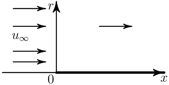
Figure 1. Streamline of a needle by the filling flow.

The first variant: an incompressible fluid. For this, the Navier–Stokes equations in independent variables $x,r$ are equivalent to a system of two PDEs for the flow function $\psi$ and pressure p:

$$\begin{array}{cc}\hfill g_1\equiv & -\frac{1}{r}\frac{\partial \psi }{\partial x}\frac{\partial }{\partial r}\left(\frac{1}{r}\frac{\partial \psi }{\partial r}\right)+\frac{1}{r}\frac{\partial \psi }{\partial r}\frac{\partial }{\partial x}\left(\frac{1}{r}\frac{\partial \psi }{\partial r}\right)+\frac{1}{\rho }\frac{\partial p}{\partial x}-\nu \left(\frac{1}{r}\frac{\partial }{\partial r}\left(r\frac{\partial }{\partial r}\left(\frac{1}{r}\frac{\partial \psi }{\partial r}\right)\right)+\frac{{\partial }^2}{\partial x^2}\left(\frac{1}{r}\frac{\partial \psi }{\partial r}\right)\right)=0,\hfill \\ \hfill g_2\equiv & \frac{1}{r}\frac{\partial \psi }{\partial x}\frac{\partial }{\partial r}\left(\frac{1}{r}\frac{\partial \psi }{\partial x}\right)-\frac{1}{r}\frac{\partial \psi }{\partial r}\frac{\partial }{\partial x}\left(\frac{1}{r}\frac{\partial \psi }{\partial x}\right)+\frac{1}{\rho }\frac{\partial p}{\partial r}+\nu \left(\frac{\partial }{\partial r}\left(\frac{1}{r}\frac{{\partial }^2\psi }{\partial x\partial r}\right)+\frac{{\partial }^2}{\partial x^2}\left(\frac{1}{r}\frac{\partial \psi }{\partial x}\right)\right)=0,\hfill \end{array}$$

(8)

where density $\rho$ and viscosity $\nu =\mathrm{const}$, with boundary conditions

$$\psi =\frac{u_{\infty }}{2}{r}^2,p=p_0\mathrm{at}x=-\infty ,u_{\infty },p_0=\mathrm{const};$$

(9)

$$\frac{\partial \psi }{\partial x}=\frac{\partial \psi }{\partial r}=\frac{{\partial }^2\psi }{\partial x\partial r}=\frac{{\partial }^2\psi }{\partial r^2}=0\mathrm{in}x⩾0,r=0.$$

(10)

The system (8) has the form (4) with $m=n=2$ and $m+n=4$. Thus, supports of Equation (8) should be considered in ${\mathbb{R}}^4$. It turns out that the polyhedra $\Gamma \left(g_1\right)$ and $\Gamma \left(g_2\right)$ of the Equation (8) are three-dimensional tetrahedrons which can be placed into one linear three-dimensional subspace by parallel transfer, which simplifies the separation of truncated systems. Analyzing the solutions of the truncated systems and the results of their jointing, it was possible to show that the system (8) has no solution with $p⩾0$ satisfying both boundary conditions (9) and (10).

The second variant: a compressible thermally conductive fluid and a nonthermally conductive needle. For this variant, the Navier–Stokes equations in independent variables $x,r$ are equivalent to a system of three PDEs for the flow function $\psi$, density $\rho$, and enthalpy h (analog of temperature):

$$\begin{array}{cc}\hfill f_1\equiv & -\frac{1}{r}\frac{\partial \psi }{\partial x}\frac{\partial }{\partial r}\left(\frac{1}{\rho r}\frac{\partial \psi }{\partial x}\right)+\frac{1}{r}\frac{\partial \psi }{\partial r}\frac{\partial }{\partial x}\left(\frac{1}{\rho r}\frac{\partial \psi }{\partial x}\right)-A\frac{\partial }{\partial r}\left(\rho h\right)+\hfill \\ \hfill & +\frac{2}{3}{C}^{\nu }\frac{\partial }{\partial r}\left(\frac{h^{\nu }}{r}\frac{\partial }{\partial r}\left(\frac{1}{\rho }\frac{\partial \psi }{\partial x}\right)\right)-\frac{2}{3}{C}^{\nu }\frac{\partial }{\partial r}\left(\frac{h^{\nu }}{r}\frac{\partial }{\partial x}\left(\frac{1}{\rho }\frac{\partial \psi }{\partial r}\right)\right)-\hfill \\ \hfill & -\frac{2C^{\nu }}{r}\frac{\partial }{\partial r}\left(h^{\nu }r\frac{\partial }{\partial r}\left(\frac{1}{\rho r}\frac{\partial \psi }{\partial x}\right)\right)+C^{\nu }\frac{\partial }{\partial x}\left(h^{\nu }\frac{\partial }{\partial r}\left(\frac{1}{\rho r}\frac{\partial \psi }{\partial r}\right)\right)-\hfill \\ \hfill & -C^{\nu }\frac{\partial }{\partial x}\left(h^{\nu }\frac{\partial }{\partial x}\left(\frac{1}{\rho r}\frac{\partial \psi }{\partial x}\right)\right)+\frac{2C^{\nu }{h}^{\nu }}{\rho r^3}\frac{\partial \psi }{\partial x}=0,\hfill \\ \hfill f_2\equiv & \phantom{-}\frac{1}{r}\frac{\partial \psi }{\partial x}\frac{\partial }{\partial r}\left(\frac{1}{\rho r}\frac{\partial \psi }{\partial r}\right)-\frac{1}{r}\frac{\partial \psi }{\partial r}\frac{\partial }{\partial x}\left(\frac{1}{\rho r}\frac{\partial \psi }{\partial r}\right)-A\frac{\partial }{\partial x}\left(\rho h\right)+\hfill \\ \hfill & +\frac{2}{3}{C}^{\nu }\frac{\partial }{\partial x}\left(\frac{h^{\nu }}{r}\frac{\partial }{\partial r}\left(\frac{1}{\rho }\frac{\partial \psi }{\partial x}\right)\right)-\frac{2}{3}{C}^{\nu }\frac{\partial }{\partial x}\left(\frac{h^{\nu }}{r}\frac{\partial }{\partial x}\left(\frac{1}{\rho }\frac{\partial \psi }{\partial r}\right)\right)+\hfill \\ \hfill & +\frac{C^{\nu }}{r}\frac{\partial }{\partial r}\left(h^{\nu }r\frac{\partial }{\partial r}\left(\frac{1}{\rho r}\frac{\partial \psi }{\partial r}\right)\right)-\frac{C^{\nu }}{r}\frac{\partial }{\partial r}\left(h^{\nu }r\frac{\partial }{\partial x}\left(\frac{1}{\rho r}\frac{\partial \psi }{\partial x}\right)\right)+\hfill \\ \hfill & +2C^{\nu }\frac{\partial }{\partial x}\left(h^{\nu }\frac{\partial }{\partial x}\left(\frac{1}{\rho r}\frac{\partial \psi }{\partial r}\right)\right)=0,\hfill \\ \hfill f_3\equiv & \phantom{-}\frac{1}{r}\frac{\partial \psi }{\partial x}\frac{\partial h}{\partial r}-\frac{1}{r}\frac{\partial \psi }{\partial r}\frac{\partial h}{\partial x}-\frac{A}{\rho r}\frac{\partial \psi }{\partial x}\frac{\partial \left(\rho h\right)}{\partial r}+\frac{A}{\rho r}\frac{\partial \psi }{\partial r}\frac{\partial \left(\rho h\right)}{\partial x}+\hfill \\ \hfill & +2C^{\nu }{h}^{\nu }{\left(\frac{\partial }{\partial r}\left(\frac{1}{\rho r}\frac{\partial \psi }{\partial x}\right)\right)}^2+2C^{\nu }{h}^{\nu }{\left(\frac{1}{r^2\rho }\frac{\partial \psi }{\partial x}\right)}^2+2C^{\nu }{h}^{\nu }{\left(\frac{\partial }{\partial x}\left(\frac{1}{\rho r}\frac{\partial \psi }{\partial r}\right)\right)}^2+\hfill \\ \hfill & +C^{\nu }{h}^{\nu }{\left(\frac{\partial }{\partial x}\left(\frac{1}{\rho r}\frac{\partial \psi }{\partial x}\right)\right)}^2-C^{\nu }{h}^{\nu }\frac{\partial }{\partial x}\left(\frac{1}{\rho r}\frac{\partial \psi }{\partial x}\right)\frac{\partial }{\partial r}\left(\frac{1}{\rho r}\frac{\partial \psi }{\partial r}\right)+\hfill \\ \hfill & +C^{\nu }{h}^{\nu }{\left(\frac{\partial }{\partial r}\left(\frac{1}{\rho r}\frac{\partial \psi }{\partial r}\right)\right)}^2-\frac{2}{3}{C}^{\nu }{h}^{\nu }{\left(\frac{1}{r}\frac{\partial }{\partial r}\left(\frac{1}{\rho }\frac{\partial \psi }{\partial x}\right)\right)}^2+\hfill \\ \hfill & +\frac{4C^{\nu }{h}^{\nu }}{3r}\frac{\partial }{\partial r}\left(\frac{1}{\rho }\frac{\partial \psi }{\partial x}\right)\frac{\partial }{\partial x}\left(\frac{1}{\rho r}\frac{\partial \psi }{\partial r}\right)-\frac{2}{3}{C}^{\nu }{h}^{\nu }{\left(\frac{\partial }{\partial x}\left(\frac{1}{\rho r}\frac{\partial \psi }{\partial r}\right)\right)}^2+\hfill \\ \hfill & +\frac{C^{\nu }}{\sigma r}\frac{\partial }{\partial r}\left(r{h}^{\nu }\frac{\partial h}{\partial r}\right)+\frac{C^{\nu }}{\sigma }\frac{\partial }{\partial x}\left(h^{\nu }\frac{\partial h}{\partial x}\right)=0,\hfill \end{array}$$

(11)

where the parameters $A,C,\sigma >0$ and $\nu \in [0,1]$, with boundary conditions

$$\psi ={\psi }_0{r}^2,\rho ={\rho }_0,h=h_0\mathrm{at}x=-\infty ,{\psi }_0,{\rho }_0,h_0=\mathrm{const}$$

(12)

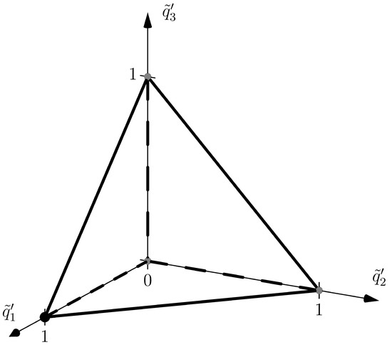
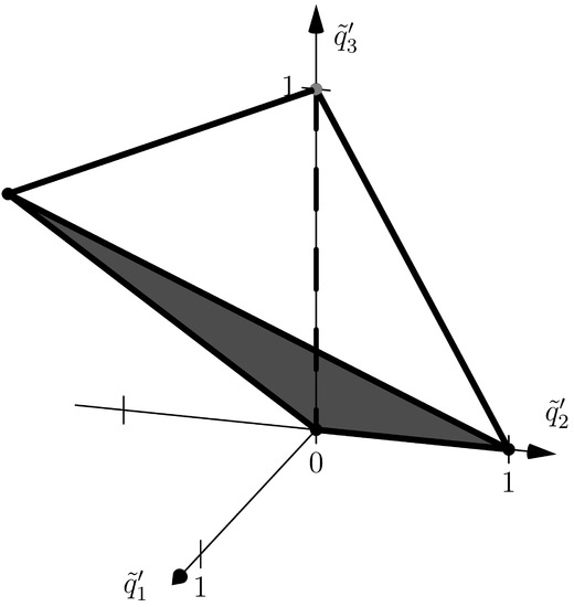
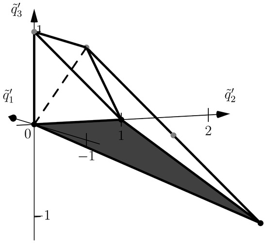
and (10). Here, $x_1=x$, $x_2=r$, $y_1=\psi$, $y_2=\rho$, $y_3=h$, so $m=2$, $n=3$, $m+n=5$. In the space ${\mathbb{R}}^5$, all polyhedra $\Gamma \left(f_1\right)$, $\Gamma \left(f_2\right)$, $\Gamma \left(f_3\right)$ of equations (11) are three-dimensional and can be shifted parallel in one linear three-dimensional subspace. In the coordinates $\left({\tilde{q}}_1^{\prime },{\tilde{q}}_2^{\prime },{\tilde{q}}_3^{\prime }\right)$ of this three-dimensional space, they are shown in Figure 2, Figure 3 and Figure 4, respectively.

Figure 2. The polyhedron $\Gamma \left(f_1\right)$ of the first equation of the system (11). The boldface point corresponds to the first equation of the truncated system (13).

Figure 3. The polyhedron $\Gamma \left(f_2\right)$ of the second equation of the system (11). The selected face corresponds to the second equation of the truncated system (13).

Figure 4. The polyhedron $\Gamma \left(f_3\right)$ of the third equation of the system (11). The selected face corresponds to the third equation of the truncated system (13).

It follows from the boundary conditions (12) that the boundary layer corresponds to a normal vector $P=(2,1,2,0,0)$. Thus, the truncated system corresponding to the boundary layer on the needle has the form:

$$\begin{array}{cc}\hfill {\widehat{f}}_{12}^{\left(0\right)}\equiv & -A\frac{\partial \left(\rho h\right)}{\partial r}=0\mathrm{or}\frac{\partial \left(\rho h\right)}{\partial r}=0,\hfill \\ \hfill {\widehat{f}}_{22}^{\left(2\right)}\equiv & \phantom{-}\frac{1}{r}\frac{\partial \psi }{\partial x}\frac{\partial }{\partial r}\left(\frac{1}{\rho r}\frac{\partial \psi }{\partial r}\right)-\frac{1}{r}\frac{\partial \psi }{\partial r}\frac{\partial }{\partial x}\left(\frac{1}{\rho r}\frac{\partial \psi }{\partial r}\right)-A\frac{\partial \left(\rho h\right)}{\partial x}+\frac{C^{\nu }}{r}\frac{\partial }{\partial r}\left(h^{\nu }r\frac{\partial }{\partial r}\left(\frac{1}{\rho r}\frac{\partial \psi }{\partial r}\right)\right)=0,\hfill \\ \hfill {\widehat{f}}_{32}^{\left(2\right)}\equiv & \phantom{-}\frac{1}{r}\frac{\partial \psi }{\partial x}\frac{\partial h}{\partial r}-\frac{1}{r}\frac{\partial \psi }{\partial r}\frac{\partial h}{\partial x}-\frac{A}{\rho r}\frac{\partial \psi }{\partial x}\frac{\partial \left(\rho h\right)}{\partial r}+\frac{A}{\rho r}\frac{\partial \psi }{\partial r}\frac{\partial \left(\rho h\right)}{\partial x}+C^{\nu }{h}^{\nu }{\left(\frac{\partial }{\partial r}\left(\frac{1}{\rho r}\frac{\partial \psi }{\partial r}\right)\right)}^2+\hfill \\ \hfill & +\frac{C^{\nu }}{\sigma r}\frac{\partial }{\partial r}\left(r{h}^{\nu }\frac{\partial h}{\partial r}\right)=0,\hfill \end{array}$$

(13)

with self-similar variables

$$\psi =xG\left(\xi \right),\rho =P\left(\xi \right),h=H\left(\xi \right),\xi =r^2/x,$$

(14)

and the boundary conditions

$$\psi ={\psi }_0{r}^2,\rho ={\rho }_0,h=h_0;{\psi }_0,{\rho }_0,h_0=\mathrm{const},r\to \infty$$

(15)

and (10). In Figure 2, Figure 3 and Figure 4, the vertex and faces corresponding to the truncated system (13) are boldfaced. According to Equations  (13)–(15), the product $P\left(\xi \right)H\left(\xi \right)=\mathrm{const}=C_0\equiv {\rho }_0{h}_0$. Thus, $P\left(\xi \right)=C_0/H\left(\xi \right)$ and the system (13), for variables (14) is equivalent to a system of two ODEs:

$$\begin{array}{cc}\hfill F_2\equiv & G{\left(G^{\prime }H\right)}^{\prime }+2C^{\nu }{\left[\xi H^{\nu }{\left(G^{\prime }H\right)}^{\prime }\right]}^{\prime }=0,\hfill \\ \hfill F_3\equiv & 2G{H}^{\prime }+16C^{\nu }{C}_0^{-2}\xi H^{\nu }{\left({\left(G^{\prime }H\right)}^{\prime }\right)}^2+4C^{\nu }{\sigma }^{-1}{\left(\xi H^{\nu }{H}^{\prime }\right)}^{\prime }=0\hfill \end{array}$$

(16)

where ${}^{\prime }\equiv d/d\xi$, with boundary conditions

$$\begin{array}{cc}\hfill G=& {\psi }_0\xi ,H=h_0\mathrm{for}\xi \to +\infty ,\hfill \end{array}$$

(17)

$$\begin{array}{cc}\hfill G=& dG/d\xi =0\mathrm{for}\xi =0.\hfill \end{array}$$

(18)

The problem (16), (17) and (18) has an invariant manifold ${\left(G^{\prime }H\right)}^{\prime }=0$, on which it reduces to one equation

$$\Delta \equiv 2{\left(\xi H^{\nu }{H}^{\prime }\right)}^{\prime }H-2\xi H^{\nu }{H^{\prime }}^2+(\xi +c_2)H^{\prime }=0,$$

where $c_2$ is an arbitrary constant, with boundary conditions

$$\begin{array}{cccc}\hfill H\to & 1\hfill & \hfill \mathrm{at}\xi & \to +\infty ,\hfill \\ \hfill H\to & +\infty \hfill & \hfill \mathrm{at}\xi & \to +0.\hfill \end{array}$$

An analysis of the solutions of the last problem by methods of planar power geometry [9] shows that for $\nu \in (0,1)$, it has solutions of the form

$$H\sim c_3{\left||\ln \xi \right|}^{1/\nu },\xi \to 0,$$

where $c_3$ is an arbitrary constant.

Thus, at $\nu \in (0,1)$ in the boundary layer $r^2/x<\mathrm{const}$ at $x\to +\infty$ and $\xi =r^2/x\to 0$, the asymptotic form of the flow is obtained:

$$\psi \sim c_1{r}^2{\left|\ln \xi \right|}^{-1/\nu },\rho \sim c_2{\left|\ln \xi \right|}^{-1/\nu },h\sim c_3{\left|\ln \xi \right|}^{1/\nu }$$

i.e., near the needle, the density decreases to zero and the temperature increases to infinity as the distance from the tip of the needle tends to plus infinity.

4. Algorithms of Power Geometry

4.1. Euler’s Algorithm and a Generalization of Continued Fraction

A matrix $\alpha$ is called unimodular if all its elements are integer and $det\alpha =\pm 1$.

Problem 1.

Let n-dimensional integer vector $A=(a_1,a_2,\cdots ,a_n)$ be given. Find an n-dimensional unimodular matrix α such that the vector $A\alpha =C=(c_1,\cdots ,c_n)$ contains only one coordinate $c_n$ different from zero.

To solve it, Euler [10] proposed the following algorithm. Firstly, let all coordinates of the vector A be non-negative. Using the permutation ${A\alpha }_0=\left({\tilde{a}}_1,{\tilde{a}}_2,\cdots ,{\tilde{a}}_n\right)$, we order the coordinates

$${\tilde{a}}_j⩽{\tilde{a}}_{j+1},j=1,\cdots ,n-1.$$

Here, ${\alpha }_0$ is a unimodular permutation matrix. Let ${\tilde{a}}_k$ be the smallest of the numbers ${\tilde{a}}_j$ different from zero.

Let

$$b_j=\left[\frac{{\tilde{a}}_j}{{\tilde{a}}_k}\right],j=1,\cdots ,n,$$

where $\left[x\right]$ is the integer part of the number x. In this case, $b_1=\cdots =b_{k-1}=0$, $b_k=1$. Let us perform the transformation

$$d_j={\tilde{a}}_j-b_j{\tilde{a}}_k,1⩽j⩽n,j\ne k,d_k={\tilde{\alpha }}_k.$$

(19)

It corresponds to a unimodular matrix ${\alpha }_1$ that has ones on the diagonal, and in the kth row are elements

$$0,0,\cdots ,0,1,-b_{k+1},\cdots ,-b_n,$$

i.e.,

$$\tilde{A}{\alpha }_1=D=(d_1,\cdots ,d_n).$$

Now we order the components of the vector D using the unimodular permutation matrix ${\beta }_0$ such that $D{\beta }_0=\tilde{D}=\left(0,\cdots ,0,{\tilde{d}}_k,\cdots ,{\tilde{d}}_n\right)$, where ${\tilde{d}}_j⩽{\tilde{d}}_{j+1}$.

Let ${\tilde{d}}_l$ be the smallest of ${\tilde{d}}_j$ different from zero, and $e_j=\left[{\tilde{d}}_j/{\tilde{d}}_l\right]$, $j=1,\cdots ,l$. We perform the transformation

$$f_j={\tilde{d}}_j-e_j{\tilde{d}}_l,1⩽j⩽n,j\ne l,f_l={\tilde{d}}_l,$$

and so on. At each step, the maximum of the coordinates of the vector decreases and is the nth coordinate. Thus, after a finite number of steps we obtain a vector with one nonzero coordinate which is the last one. Its value is the GCD of all initial coordinates $a_1,\cdots ,a_n$. Each step consists of a permutation matrix and a triangular matrix with a unit diagonal:

$$A{\alpha }_0{\alpha }_1{\beta }_0{\beta }_1{\gamma }_0{\gamma }_1\cdots {\omega }_0{\omega }_1=A\alpha =C=(0,\cdots ,0,c_n).$$

Matrix

$$\alpha ={\alpha }_0{\alpha }_1{\beta }_0{\beta }_1{\gamma }_0{\gamma }_1\cdots {\omega }_0{\omega }_1$$

(20)

is the solution to Problem 1.

If not all coordinates $a_j$ of the original vector A are of the same sign, then we first order them by modulo

$$\left|{\tilde{a}}_j\right|⩽\left|{\tilde{a}}_{j+1}\right|$$

and suppose

$$b_j=[\left|{\tilde{a}}_j\right|/\left|{\tilde{a}}_k\right|]sign{\tilde{a}}_{j}sign\widetilde{a_k}.$$

Remark 1.

By multiplying the matrix α on the right by a unimodular permutation matrix, we can obtain a vector from vector C that has all but one coordinate equal to zero, and a single nonzero coordinate located at any position.

4.2. Power Transformations

To simplify a truncated system (5) and any quasi-homogeneous system, it is convenient to use a power transformation. Let $\alpha$ be a square real nondegenerate block matrix of dimension $m+n$ of the form

$$\alpha =\left(\begin{array}{cc}{\alpha }_{11}& {\alpha }_{12}\\ 0& {\alpha }_{22}\end{array}\right),$$

(21)

where ${\alpha }_{11}$ and ${\alpha }_{22}$ are square matrices of sizes m and n, respectively. We denote $\ln Z=\left(\ln z_1,\cdots ,\ln z_{m+n}\right)$, and by the asterisk ${}^{*}$ we denote transposition.

Transformation of the variables

$$\ln W=\left(\ln Z\right)\alpha$$

(22)

is called power transformation.

Theorem 2

([1]). The power transformation (22) changes a differential monomial $a\left(Z\right)$ with exponent of degree $Q\left(a\right)$ into a differential sum $b\left(W\right)$ with exponent of degree $Q\left(b\right)$:

$$R=Q\left(b\right)=Q\left(a\right){\alpha }^{-1*}.$$

(23)

Corollary 1.

The power transformation (22) changes the differential sum (3) with support $\mathbf{S}\left(f\right)$ into the differential sum $g\left(W\right)$ with support

$$\mathbf{S}\left(g\right)=\mathbf{S}\left(f\right){\alpha }^{-1*},$$

i.e.,

$$\mathbf{S}\left(f\right)=\mathbf{S}\left(g\right){\alpha }^{*}$$

(24)

Theorem 3

([1]). If the system (4) is a quasi-homogeneous system and $d=dim\tilde{\mathbf{\Gamma }}$, then there exist a power transformation (22) and monomials $Z^{T_i}$, $i=1,\cdots ,n$ which change the system (4) into the system

$$g_i\left(W\right)\equiv Z^{T_i}{f}_i\left(Z\right)=0,i=1,\cdots ,n,$$

where all $g_i\left(W\right)$ are differential sums, and all their supports $\mathbf{S}\left(g_i\right)$ have $m+n-d$ identical coordinates $q_j$ equal to zero.

Usually, the supports of differential equations are integer. For them, it is desirable to have power transformations that preserve the integrability of the supports. This property is possessed by power transformations (22) with a unimodular matrix $\alpha$ in which all elements are integers and $det\alpha =\pm 1$. For a unimodular matrix $\alpha$, its inverse ${\alpha }^{-1}$ and transpose ${\alpha }^{*}$ matrices are also unimodular.

Let us compute the unimodular matrix (21) of the power transformation (22) in one important case. Suppose that in the system (4) all supports $\mathbf{S}\left(f_1\right),\cdots ,\mathbf{S}\left(f_n\right)$ are integers and the normal to them is an integer vector $N=({\nu }_1,\cdots ,{\nu }_{m+n})\ne 0$, i.e., for all $Q\in \mathbf{S}\left(f_i\right)$ we have $⟨Q,N⟩={\lambda }_i$, $i=1,\cdots ,n$. Split the vector N into two parts: $N_1=({\nu }_1,\cdots ,{\nu }_m)$ and $N_2=({\nu }_{m+1},\cdots ,{\nu }_{m+n})$, and perform the same for the vector $Q=(Q_1,Q_2)$.

Consider three cases:

(1)

$N_1=0$, $N_2\ne 0$, then $⟨Q_2,N_2⟩={\lambda }_i$;

(2)

$N_1\ne 0$, $N_2=0$, then $⟨Q_1,N_1⟩={\lambda }_i$;

(3)

$N_1\ne 0$, $N_2\ne 0$.

Below, I is the unit matrix.

Lemma 1.

In the case 1, there exists a unimodular matrix ${\alpha }_{22}$ of size n such that, after transformation (22) with ${\alpha }_{11}=I$, ${\alpha }_{12}=0$ in each transformed differential sum $g_i\left(W\right)$, the coordinate $w_{m+n}$ is contained only in a fixed degree ${\tilde{\lambda }}_i$.

Proof of Lemma 1.

Using the Euler algorithm from Section 4.1 for the vector $N_2$, we find such a unimodular matrix ${\alpha }_{22}$ of size n that

$$N_2{\alpha }_{22}=(0,\cdots ,0,{\mu }_2),$$

and ${\mu }_2$ is GCD of numbers ${\nu }_{m+1},\cdots ,{\nu }_{m+n}$. According to (23) and (24) for $Q\in \mathbf{S}\left(f_i\right)$ we have

$${\lambda }_i=⟨N_2,Q_2⟩=⟨N_2,R_2{\alpha }_{22}^{*}⟩=⟨N_2{\alpha }_{22},R_2⟩={\mu }_2{r}_{m+n}.$$

Then, ${\tilde{\lambda }}_i={\lambda }_i/{\mu }_2$. The proof is over.    □

Lemma 2.

In the case 2, there exists a unimodular matrix ${\alpha }_{11}$ of size m such that after transformation (22) with ${\alpha }_{22}=I$, ${\alpha }_{21}=0$ in each transformed differential sum $g_i\left(W\right)$, the coordinate $w_m$ contains only a fixed degree ${\tilde{\lambda }}_i$.

The proof is the same as the proof of Lemma 1.

Lemma 3.

In the case 3, if $gcd{N}_2/gcd{N}_1=\omega$ is an integer, then there exists such a unimodular matrix α of (21) that every differential sum $g_i\left(W\right)$ contains the coordinate $w_m$ only in a fixed degree ${\tilde{\lambda }}_i$.

Proof of Lemma 3.

Let

$${\mu }_i=gcd{N}_i,i=1,2.$$

By Euler’s algorithm, we obtain the representations

$$N_i{\beta }_i=(0,\cdots ,0,{\mu }_i),i=1,2,$$

where ${\beta }_i$ are unimodular matrices of sizes m and n, respectively. In other words,

$$N\beta =(0,\cdots ,{\mu }_1,0,\cdots ,{\mu }_2)\equiv M={\mu }_1(0,\cdots ,1,0,\cdots ,\omega ),$$

where $\beta$ is a block unimodular matrix

$$\beta =\left(\begin{array}{cc}{\beta }_1& 0\\ 0& {\beta }_2\end{array}\right)$$

Then, we have

$$M(I-\gamma )=(0,\cdots ,{\mu }_1,0,\cdots ,0),$$

where I is a unit matrix of size $m+n$, and the matrix $\gamma =\left({\gamma }_{ij}\right)$ has a single nonzero element ${\gamma }_{m,m+n}=\omega$. Then the matrix $\alpha =\beta (I-\gamma )$ is unimodular, has a block structure (21), and each differential sum $g_i\left(W\right)$ contains the coordinate $w_m$ in degree $\tilde{\lambda }={\lambda }_i/{\mu }_1$. Reducing each of them by the value of $w_m^{{\tilde{\lambda }}_i}$, we obtain a system in which the variable $w_m$ is contained with zero-degree exponent. The proof is over.    □

Remark 2.

If the relation ω is not integer, we can still perform a degree transformation of Lemma 3, but the support of the transformed system will not be integer.

4.3. Logarithmic Transformation

Let $z_j$ be one of the coordinates $x_k$ or $y_l$ according to the beginning of Section 2. Transformation:

$${\zeta }_j=\ln z_j$$

(25)

Let us call this logarithmic transformation.

Theorem 4

([11]). Let $f\left(Z\right)$ be such a differential sum that for all its monomials, jth component of $q_j$ vector degree exponent $Q=(q_1,\cdots ,q_{m+n})$ is zero, then as a result of the logarithmic transformation (25), a differential sum $f\left(Z\right)$ transforms into a differential sum from $z_1,\cdots ,{\zeta }_j,\cdots ,z_n$.

In the system

$$f_i(X,Y)=0,i=1,\cdots ,n,$$

(26)

let all $f_i$ be differential sums. Let some of its truncated system be

$${\widehat{f}}_i(X,Y)=0,i=1,\cdots ,n.$$

(27)

It is quasi-homogeneous in dimension $d<m+n$. According to Theorem 3 there exists a power transformation (22) which reduces the system (27) to the system

$$g_i\left(W\right)=0,i=1,\cdots ,n,$$

(28)

in which all supports of sums $g_i\left(W\right)$ have $m+n-d$ zero coordinates. A logarithmic transformation can be applied to these coordinates, which by theorem 4 will reduce the system (28) to the form

$$h_i\left(\tilde{W}\right)=0,i=1,\cdots ,n,$$

(29)

where $h_i$ are differential sums, and ${\tilde{w}}_j=w_j$ or $\ln w_j$, $j=1,\cdots ,m+n$. In the system (29) we can again select truncated systems and so on.

For $z_j\to 0$ or ∞, the coordinate ${\zeta }_j=\ln w_j$ always tends to $\pm \infty$. If we are interested only in those solutions (7) which have a normal cone $\mathbf{u}$ intersecting a given cone K, then the cone K is called the cone of problem. Thus, after the logarithmic transformation (25) for the coordinate ${\zeta }_j$ in the cone of the problem, we have $p_j⩾0$.

In the following, we will not consider all possible truncated systems (5), but only those in which one of the equations has dimension $d_i=m+n-1$. The calculations show that in this case the above procedure will cover all the truncated systems. Finally, it is convenient to combine the power and logarithmic transformations. Namely, the logarithmic transformation is performed for the coordinate $w_{m+n}$ in the case 1 and for the coordinate $w_m$ in the cases 2 and 3 of Section 4.2.

4.4. System of Notations

The original system is denoted by S, and its equations by $E1S$ and $E2S$, respectively. For the equations of the system S, the polyhedrons, normal cones, are calculated and the corresponding shortened systems are found by them, which are denoted as $S\left(1\right)$, $S\left(2\right)$, etc. For the truncated system $S\left(k\right)$, a power and/or logarithmic transformation is applied, the result of which is the system $P\left(k\right)$. The corresponding truncations of the system $P\left(k\right)$ are denoted by $S(k,1)$, $S(k,2)$, etc., and the results of their power-logarithmic transformations are denoted by $P(k,1)$, $P(k,2)$, etc. If new truncations are required, the corresponding systems are denoted as $S(k,l,m)$, and the results of the power-logarithmic transformations are denoted as $P(k,l,m)$. This branching procedure stops when one obtains a system that is solvable explicitly. Each system $S\left(m\right)$ has its cone of problem $K\left[S\right(m\left)\right]$. In the following Section 5, Section 6 and Section 7, the vectors are denoted in square brackets $[x_1,\cdots ,x_m]$, as is usual in Maple.

4.5. About the Computation of the Objects of Power Geometry

The computer algebra system Maple 2021 [12] was used for calculations in this work. A library of procedures based on the PolyhedralSets CAS Maple package was developed to implement the algorithms of power geometry. The library includes calculation procedures:

• Vector degree exponent Q of the differential monomial $a\left(Z\right)$ for a given order of independent and dependent variables.
• Of the support $\mathbf{S}$ of a partial differential equation written as a sum of differential monomials.
• Newton’s polyhedron $\mathbf{\Gamma }$ in the form of a graph of generalized faces ${\mathbf{\Gamma }}_j^{\left(d\right)}$ of all dimensions d for the given support of the equation (see below Figure 5 and Figure 6); the number j is given by the program; each generalized face has its own number j; each line of the graph contains all generalized faces ${\mathbf{\Gamma }}_j^{\left(d\right)}$ of the same dimension d, the first line contains the Newton’s polyhedron $\mathbf{\Gamma }$, the next line contains all faces ${\mathbf{\Gamma }}_j^{(m+n-1)}$ of dimension $m+n-1$ and so on; the last line contains the empty set; if ${\mathbf{\Gamma }}_j^{\left(d\right)}\subset {\mathbf{\Gamma }}_k^{(d+1)}$, then they are connected by an arrow. In ([1], Ch. 1, Section 1), “the structural diagram” was used that is similar to the graph and differs from it in two properties: numeration of faces ${\mathbf{\Gamma }}_j^{\left(d\right)}$ is independent for each dimension d and arrows are replaced by segments (see also [13]).
  

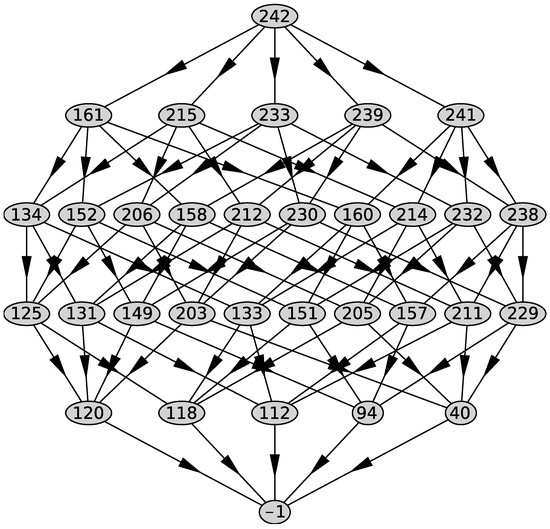  Figure 5. Graph of the polyhedron $\mathbf{\Gamma }\left(E1S\right)$ of Equation (48).
  

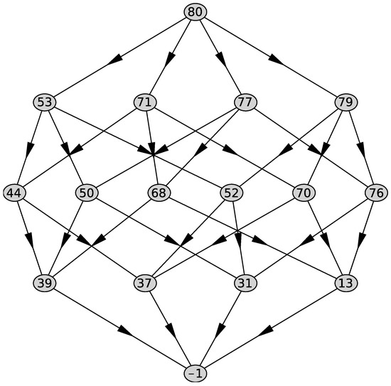  Figure 6. Graph of the polyhedron $\mathbf{\Gamma }\left(E2S\right)$ of Equation (49).
• Of the normal vector $N_j$ for the each generalized face ${\mathbf{\Gamma }}_j^{(m+n-1)}$ for the second line of the graph;
• Of the truncated equation ${\widehat{f}}_j^{\left(d\right)}=0$ by the given number j of the generalized face.
• Of the truncated equation ${\widehat{f}}_j^{\left(d\right)}=0$ by a given normal vector $N_j$, if $d=m+n-1$.
• Of the normal cone of the corresponding generalized face: if the face

  $${\mathbf{\Gamma }}_j^{\left(d\right)}={\mathbf{\Gamma }}_i^{(m+n-1)}\cap {\mathbf{\Gamma }}_k^{(m+n-1)}\cap \cdots \cap {\mathbf{\Gamma }}_l^{(m+n-1)},$$

  then the normal cone ${\mathbf{U}}_j^{\left(d\right)}$ is the conic hull of the normals $N_i,N_k,\cdots ,N_l$.
• To calculate the power or logarithmic transformation of the original variables by a given normal N of the hyperface. For this purpose, the algorithms for constructing the unimodular matrix described in Section 4.1 are used.

5. The $\mathit{k}$–$\mathit{\epsilon }$ Model of Evolution of Turbulent Bursts

According to [14,15,16,17], the model is described by the system

$$\begin{array}{cc}\hfill & k_t={\left(\frac{k^2}{\epsilon }{k}_x\right)}_x-\epsilon ,\hfill \\ \hfill & {\epsilon }_t={\left(\frac{k^2}{\epsilon }{\epsilon }_x\right)}_x-\gamma \frac{{\epsilon }^2}{k}.\hfill \end{array}$$

(30)

Here, time t and coordinate x are independent variables, the turbulent density k and the dissipation rate $\epsilon$ are dependent variables, and $\gamma$ is a real parameter. Here, $m=n=2$, $m+n=4$ and $x_1=t$, $x_2=x$, $y_1=k$, $y_2=\epsilon$.

The support of the first equation ${\mathbf{S}}_1$ of the system (30) consists of points

$$Q_1=[-1,0,1,0],Q_2=[0,-2,3,-1],Q_3=[0,0,0,1].$$

The support of the second equation ${\mathbf{S}}_2$ of the system (30) consists of points

$$Q_4=[-1,0,0,1],Q_5=[0,-2,2,0],Q_6=[0,0,-1,2].$$

The shifted supports ${\tilde{\mathbf{S}}}_1={\mathbf{S}}_1-Q_3$ and ${\tilde{\mathbf{S}}}_2={\mathbf{S}}_2-Q_6$ consist of three points:

$$\begin{array}{cc}\hfill R_1& \equiv Q_1-Q_3=Q_4-Q_6=[-1,0,1,-1],\hfill \\ \hfill R_2& \equiv Q_2-Q_3=Q_5-Q_6=[0,-2,3,-2],\hfill \\ \hfill 0& =Q_3-Q_3=Q_6-Q_6.\hfill \end{array}$$

Therefore, $d=2$.

According to Theorem 3 let us introduce new dependent variables:

$$u=Z^{R_1}=t^{-1}k{\epsilon }^{-1},v=Z^{R_2}=x^{-2}{k}^3{\epsilon }^{-2}.$$

Then

$$k=\frac{x^{2}v}{t^2{u}^2},\epsilon =\frac{x^{2}v}{t^3{u}^3}.$$

(31)

This is a power transformation (22) with matrix (21), where

$${\alpha }_{11}=\left(\begin{array}{cc}1& 0\\ 0& 1\end{array}\right),{\alpha }_{12}=\left(\begin{array}{cc}-1& 0\\ 0& -2\end{array}\right),{\alpha }_{22}=\left(\begin{array}{cc}1& 3\\ -1& -2\end{array}\right).$$

This power transformation is constructed directly on the support of the system such that it lies in the coordinate plane. The theory of Section 4.2 is not used here.

Change of the variables (31) leads the system (30) to the form

$$\begin{array}{cc}\hfill ut{\left(\ln v\right)}_t-2u-2t{u}_t=& v\left(6-12U+7V+6U^2-7UV+2V^2-2x{U}_x+x{V}_x\right)-1,\hfill \\ \hfill ut{\left(\ln v\right)}_t-3u-3t{u}_t=& v\left(6-17U+7V+12U^2-10UV+2V^2-3x{U}_x+x{V}_x\right)-\gamma ,\hfill \end{array}$$

(32)

where $U=x{\left(\ln u\right)}_x$, $V=x{\left(\ln v\right)}_x$.

Let us find the self-similar solutions of this system. Consider two cases.

The first case: $u,v$ are constants. Then, the system (32) has the form

$$\begin{array}{cc}\hfill -2u& =6v-1,\hfill \\ \hfill -3u& =6v-\gamma .\hfill \end{array}$$

(33)

Its solution

$$u=\gamma -1,v=(3-2\gamma )/6$$

(34)

has two critical values: $\gamma =1$ and $\gamma =3/2$.

The second case: Let $\zeta =t^{\sigma }x$, where $\sigma \in \mathbb{R}$. Now u and v are functions of $\zeta$. In this case, in the matrix (21), the submatrix

$${\alpha }_{11}=\left(\begin{array}{cc}1& \sigma \\ 0& 1\end{array}\right)$$

and the submatrices ${\alpha }_{21}$ and ${\alpha }_{22}$ are the same as before. For $u\left(\zeta \right)$ and $v\left(\zeta \right)$, the system (32) after substitutions

$$\frac{\partial }{\partial t}=\frac{d}{d\zeta }\frac{\partial \zeta }{\partial t}=\frac{\sigma \zeta }{t}\frac{d}{d\zeta },\frac{\partial }{\partial x}=\frac{d}{d\zeta }\frac{\partial \zeta }{\partial x}=\frac{\zeta }{x}\frac{d}{d\zeta }$$

generates a one-parameter by $\sigma$ family of systems of two ODEs:

$$\begin{array}{cc}\hfill \sigma u\zeta {\left(\ln v\right)}_{\zeta }-2u-2u\zeta u_{\zeta }=& v\left(6-12U+7V+6U^2-7UV+2V^2-2\zeta U_{\zeta }+\zeta V_{\zeta }\right)-1,\hfill \\ \hfill \sigma u\zeta {\left(\ln v\right)}_{\zeta }-3u-3\zeta u_{\zeta }=& v\left(6-17U+7V+12U^2-10UV+2V^2-3\zeta U_{\zeta }+\zeta V_{\zeta }\right)-\gamma ,\hfill \end{array}$$

(35)

where $U=\zeta {\left(\ln u\right)}_{\zeta }$, $V=\zeta {\left(\ln v\right)}_{\zeta }$.

If u and v are functions only of t, then from (32) we obtain the system of ODES:

$$\begin{array}{cc}\hfill ut{\left(\ln v\right)}_t-2u-2t{u}_t& =6v-1,\hfill \\ \hfill ut{\left(\ln v\right)}_t-3u-3t{u}_t& =6v-\gamma .\hfill \end{array}$$

(36)

For its solutions

$$u=w/t$$

(37)

and, if $\gamma \ne 1$, $\gamma \ne 3/2$, then

$$v=\frac{2\gamma -3}{-6+\beta w^{(3-2\gamma )/(\gamma -1)}},$$

(38)

where $w=(\gamma -1)t+\alpha$ and $\alpha$, $\beta$ are constants.

For $\gamma =1$

$$v=\frac{1}{6+\beta exp(t/\alpha )}.$$

(39)

For $\gamma =3/2$

$$v=\frac{1}{\beta -12\ln (\alpha +t/2)}.$$

(40)

Let $\gamma \ne 1$, $\gamma \ne 3/2$, and $u=\gamma -1+\alpha /t$. Find solutions of the system (32) of the form $v(t,x)=v_p\left(t\right)x^p$ with $p\ne 0$. For them, $U=0$, $V=p$, and $V_x=0$ and equations (32) reduce to one equation:

$$ut{\left(\ln v_p\right)}_t=v_p{x}^p\left(6+7p+2p^2\right)+3-2\gamma .$$

Here, the first and last terms are of order zero on x, and the middle term is of order $p\ne 0$. Consequently, this equation has a solution only if the middle term is zero, i.e.,

$$6+7p+2p^2=0.$$

This equation has two roots: $p=-2$, $p=-3/2$. Moreover, for these values of p it is possible to find a solution of the system (32) of the form

$$v(t,x)=v_0\left(t\right)+v_p\left(t\right)x^p,$$

where $v_0\left(t\right)$ is the solution (38) of the system (36). Here, for $v_p$, we obtain the equation

$$ut{\left(\ln v_p\right)}_t=-\left(7p+3p^2\right)v_0+2\gamma -3.$$

(41)

Here, the coefficient

$$-\left(7p+3p^2\right)=\left\{\begin{array}{cc}2,\hfill & \mathrm{if}p=-2,\hfill \\ 15/4,\hfill & \mathrm{if}p=-3/2.\hfill \end{array}\right.$$

Thus, it is proven.

Theorem 5.

The system (32) reduces to a finite dimensional ODE system in three cases:

1. 

To a one-parameter family of two Equations (35);

2. 

To a system of three Equations (36) and (41) with $p=-2$;

3. 

To the system of three Equations (36) and (41) with $p=-3/2$.

Up to now, only solutions to the case 2 at $u=\gamma -1$ have been known, i.e., solutions to the two-dimensional system of ODEs (see [15,16,17,18]).

Theorem 6.

The system (32) has a one-parameter by α family of solutions:

$$u=\frac{\alpha x^p}{t},p=\frac{12\gamma -17\pm \sqrt{24\gamma +1}}{12(\gamma -2)},v=\frac{25+12\gamma \mp 7\sqrt{24\gamma +1}}{12},$$

where α is an arbitrary constant.

Proof of Theorem 6.

Here, $v_t=0$, $u+t{u}_t=0$, $U=p$, $V=0$, $U_x=0$, $V_x=0$. Thus, the Equation (32) take the form

$$\begin{array}{cc}\hfill v\left(6-12p+6p^2\right)& =6v{(p-1)}^2=1,\hfill \\ \hfill v\left(6-17p+12p^2\right)& =v(4p-3)(3p-2)=\gamma .\hfill \end{array}$$

Substituting the specified values of p and v here, we obtain two identities. □

If in (32) u and v are functions only of x, then they satisfy the system of ODEs:

$$\begin{array}{cc}\hfill -2u=& v\left(6-12U+7V+6U^2-7UV+2V^2-2U_{x}x+V_{x}x\right)-1,\hfill \\ \hfill -3u=& v\left(6-17U+7V+12U^2-10UV+2V^2-3U_{x}x+V_{x}x\right)-\gamma .\hfill \end{array}$$

(42)

This is a particular case of the family (35) at $\sigma =0$.

Below, we assume that each intermediate variable is different from identical zero. Thus, we can consider its logarithm.

After the logarithmic transformation,

$$\tau =\ln t,\xi =\ln x$$

(43)

the system (32) takes the form

$$\begin{array}{cc}\hfill u{\left(\ln v\right)}_{\tau }-2u-2u_{\tau }& =v\left(6-12U+7V+6U^2-7UV+2V^2-2U_{\xi }+V_{\xi }\right)-1,\hfill \end{array}$$

(44)

$$\begin{array}{cc}\hfill u{\left(\ln v\right)}_{\tau }-3u-3u_{\tau }& =v\left(6-17U+7V+12U^2-10UV+2V^2-3U_{\xi }+V_{\xi }\right)-\gamma ,\hfill \end{array}$$

(45)

where $U={\left(\ln u\right)}_{\xi }$, $V={\left(\ln v\right)}_{\xi }$.

Below, all computations are performed for the system S consisting of a linear combination of the original equations:

1

Equation $E1S$ is the difference of the Equations (44) and (45);

2

Equation $E2S$ is the difference of the tripled Equation (44) and the doubled Equation (45).

As a result, the S system takes the form

$$\begin{array}{cc}\hfill u+u_{\tau }& =5vU-7v{U}^2+3U{v}_{\xi }+v{U}_{\xi }+\gamma -1,\hfill \end{array}$$

(46)

$$\begin{array}{cc}\hfill u{\left(\ln v\right)}_{\tau }& =6v-2vU+7v_{\xi }-6v{U}^2+U{v}_{\xi }+v_{\xi }V+v_{\xi \xi }+2\gamma -3.\hfill \end{array}$$

(47)

To apply the Section 4.5 procedures, Equations (46) and (47) of the S system are rewritten as a sum of differential monomials:

$$\begin{array}{cc}\hfill E1S\equiv & u^3+\left(u_{\tau }\right)u^2-\gamma u^2-5v\left(u_{\xi }\right)u-v\left(u_{\xi ,\xi }\right)u-3\left(u_{\xi }\right)\left(v_{\xi }\right)u+7v{\left(u_{\xi }\right)}^2+u^2=0,\hfill \end{array}$$

(48)

$$\begin{array}{cc}\hfill E2S\equiv & u^3\left(v_{\tau }\right)-\left(v_{\xi ,\xi }\right)v{u}^2-6v^2{u}^2-7\left(v_{\xi }\right)v{u}^2-2\gamma v{u}^2-{\left(v_{\xi }\right)}^2{u}^2+\hfill \\ \hfill & +2v^2\left(u_{\xi }\right)u+\left(u_{\xi }\right)\left(v_{\xi }\right)vu+6v^2{\left(u_{\xi }\right)}^2+3v{u}^2=0.\hfill \end{array}$$

(49)

The supports of Equations (48) and (49) are

$$\begin{array}{cc}\hfill \mathbf{S}\left(E1S\right)=& \left\{\right[-1,0,3,0],[0,-2,2,1],[0,-1,2,1],[0,0,2,0],[0,0,3,0\left]\right\},\phantom{111}\hfill \end{array}$$

(50)

$$\begin{array}{cc}\hfill \mathbf{S}\left(E2S\right)=& \left\{\right[-1,0,3,1],[0,-2,2,2],[0,-1,2,2],[0,0,2,1],[0,0,2,2\left]\right\}.\hfill \end{array}$$

(51)

To perform computations with a convex polyhedron of large dimension n, it is convenient to represent the latter as an oriented graph, all vertices of which have a unique number j (identifier) and correspond to a generalized face ${\mathbf{\Gamma }}_j^{\left(d\right)}$ of appropriate dimension d. The top vertex of the graph contains the polyhedron $\mathbf{\Gamma }$ itself, the next level contains generalized faces ${\mathbf{\Gamma }}_k^{(n-1)}$ of dimension $n-1$, below are generalized faces ${\mathbf{\Gamma }}_k^{(n-2)}$ of dimension $n-2$, and so on. The lowest vertex of the graph is an empty set. The segments connecting vertices of the graph mean that the lower element (the generalized edge) lies in the upper one (the generalized edge of higher dimension). The alternative sum of the number of vertices of the graph in the lines is equal to zero.

The graph of the polyhedron $\mathbf{\Gamma }\left(E1S\right)$ computed by support (50) is shown in Figure 5. The alternative sum of the numbers of elements in the rows is $1-5+10-10+5-1=0$. The polyhedron $\mathbf{\Gamma }\left(E1S\right)$ is a four-dimensional simplex and has five three-dimensional faces with identifiers $161,215,233,239,241$, computed by the program. They correspond to the external normals

$$\begin{array}{c}{N}_{161}^{\left(3\right)}=[1,0,0,0],N_{215}^{\left(3\right)}=[-1,0,-1,0],N_{233}^{\left(3\right)}=[0,0,1,1],\\ N_{239}^{\left(3\right)}=[0,1,0,1],N_{241}^{\left(3\right)}=[0,-1,0,-2].\end{array}$$

The graph of the polyhedron $\mathbf{\Gamma }\left(E2S\right)$ computed by support (51) is shown in Figure 6. The polyhedron $\Gamma \left(E2S\right)$ lies in a three-dimensional plane with the normal

$$N_{80}^{\left(3\right)}\left(E2S\right)=[1,0,1,0]$$

and is a three-dimensional simplex, i.e., the Equation (49) is quasi-homogeneous.

Let us construct all truncations corresponding to the cone of problem $K\left[S\right]=\{p_1,p_2⩾0\}$ according to change (43). The normals $N_{161}^{\left(3\right)}$, $N_{233}^{\left(3\right)}$, $N_{239}^{\left(3\right)}$, and $N_{80}^{\left(3\right)}$ fall into the cone of problem $K\left[S\right]$. For each of the mentioned normals, we compute the truncations of the system (48), (49) and reject trivial, i.e., those consisting of a single algebraic monomial.

The truncation of Equation (49) corresponding to the normal $N_{239}^{\left(3\right)}$ and the truncation of Equation (48) corresponding to the normal $N_{80}^{\left(3\right)}$ consist of one algebraic monomial $-6u^2{v}^2$ and $u^3$, respectively. There remain two nontrivial truncations, which we denote according to the notation system of Section 4.4 by $S\left(1\right)$ and $S\left(2\right)$.

The truncated system $S\left(1\right)$ depends on the variables $\xi$, u, v and is the system of ODEs, and cone of problem $K\left[S\left(1\right)\right]=\{p_1⩾0\}$. The equations of the system have the form:

$$\begin{array}{cc}\hfill E1S\left(1\right)\equiv & u^3-\gamma u^2-5v\left(u_{\xi }\right)u-v\left(u_{\xi ,\xi }\right)u-3\left(u_{\xi }\right)\left(v_{\xi }\right)u+7v{\left(u_{\xi }\right)}^2+u^2=0,\hfill \end{array}$$

(52)

$$\begin{array}{cc}\hfill E2S\left(1\right)\equiv & (3-2\gamma )v{u}^2+6v^2{\left(u_{\xi }\right)}^2+\left(u_{\xi }\right)\left(v_{\xi }\right)vu+2v^2\left(u_{\xi }\right)u-\hfill \\ \hfill & -{\left(v_{\xi }\right)}^2{u}^2-7\left(v_{\xi }\right)v{u}^2-6v^2{u}^2-\left(v_{\xi ,\xi }\right)v{u}^2=0.\hfill \end{array}$$

(53)

The truncated system of PDEs $S\left(2\right)$ depends on the variables $\tau$, $\xi$, u, v, and the cone of problem $K\left[S\left(2\right)\right]=\{p_1,p_2⩾0\}$. The equations of the system have the form:

$$\begin{array}{cc}\hfill E1S\left(2\right)\equiv & \left(u_{\tau }\right)u^2+u^3-5v\left(u_{\xi }\right)u-v\left(u_{\xi ,\xi }\right)u-3\left(u_{\xi }\right)\left(v_{\xi }\right)u+7v{\left(u_{\xi }\right)}^2=0,\phantom{1111}\hfill \end{array}$$

(54)

$$\begin{array}{cc}\hfill E2S\left(2\right)\equiv & 6v^2{\left(u_{\xi }\right)}^2+\left(u_{\xi }\right)\left(v_{\xi }\right)vu+2v^2\left(u_{\xi }\right)u-{\left(v_{\xi }\right)}^2{u}^2-7\left(v_{\xi }\right)v{u}^2-\hfill \\ \hfill & -6v^2{u}^2-\left(v_{\xi ,\xi }\right)v{u}^2+u^3\left(v_{\tau }\right)=0.\hfill \end{array}$$

(55)

6. Asymptotic Forms of Solutions to the System $\mathit{S}\left(\mathbf{1}\right)$

Consider the computation of asymptotic forms of solutions to the system of ODEs $S\left(1\right)$ in which Equations (52) and (53) depend on variables $\xi$, u, v, i.e., all corresponding objects of the power geometry are three-dimensional, and the cone of problem $K\left[S\left(1\right)\right]=\{p_1⩾0\}$.

The supports of the Equations (52) and (53) are

$$\begin{array}{cc}\hfill \mathbf{S}\left(E1S\right(1\left)\right)& =\left\{[-2,2,1],[-1,2,1],[0,2,0],[0,3,0]\right\},\hfill \end{array}$$

(56)

$$\begin{array}{cc}\hfill \mathbf{S}\left(E2S\right(1\left)\right)& =\left\{[-2,2,2],[-1,2,2],[0,2,1],[0,2,2]\right\}.\hfill \end{array}$$

(57)

The convex polyhedron $\mathbf{\Gamma }\left(E1S\right(1\left)\right)$ is a tetrahedron, i.e., a three-dimensional simplex with normals to two-dimensional faces, computed by the program,

$$\begin{array}{c}{N}_{53}^{\left(2\right)}=[0,1,1],N_{71}^{\left(2\right)}=[0,-1,0],N_{77}^{\left(2\right)}=[1,0,1],N_{79}^{\left(2\right)}=[-1,0,-2].\end{array}$$

The convex polyhedron $\mathbf{\Gamma }\left(E2S\right(1\left)\right)$ is a two-dimensional simplex, i.e., the left-hand side of the Equation (53) is a quasi-homogeneous differential sum. The corresponding normals are

$$\begin{array}{c}{N}_{71}^{\left(2\right)}=[0,-1,0],N_{72}^{\left(2\right)}=[0,1,0].\end{array}$$

Suitable normals are those with numbers 53, 71, 77, 72. The corresponding truncated systems are $S(1,1)$, $S(1,2)$, $S(1,3)$, and $S(1,4)$.

The shortened system $S(1,3)$ contains the trivial shortened equation $E2S(1,3)\equiv -6u^2{v}^2=0$, and the shortened system $S(1,4)$ contains the trivial equation $E1S(1,4)\equiv u^3=0$. Therefore, we do not consider these systems below.

6.1. Analysis of the Truncated System $S(1,1)$

Making truncation for the normal vector $N_{53}^{\left(2\right)}=[0,1,1]$, we obtain a system $S(1,1)$ with equations

$$\begin{array}{cc}\hfill E1S(1,1)\equiv & 7v{\left(u_{\xi }\right)}^2-3\left(u_{\xi }\right)\left(v_{\xi }\right)u-v\left(u_{\xi ,\xi }\right)u-5v\left(u_{\xi }\right)u+u^3=0,\hfill \end{array}$$

(58)

$$\begin{array}{cc}\hfill E2S(1,1)\equiv & 6v^2{\left(u_{\xi }\right)}^2+\left(u_{\xi }\right)\left(v_{\xi }\right)vu+2v^2\left(u_{\xi }\right)u-{\left(v_{\xi }\right)}^2{u}^2-7\left(v_{\xi }\right)v{u}^2-\hfill \\ \hfill & -6v^2{u}^2-\left(v_{\xi ,\xi }\right)v{u}^2=0.\hfill \end{array}$$

(59)

The normal vector $N_{53}^{\left(2\right)}=[0,1,1]$ refers to the case 1 of Section 4.2 and by Lemma 1 defines a power-logarithmic substitution

$$u=rv,s=\ln v,$$

(60)

converting after reducing Equation (58) by $v^3$ and Equation (59) by $v^4$ of system $S(1,1)$ into system $P(1,1)$ with respect to variables $\xi$, r, s with equations

$$\begin{array}{cc}\hfill E1P(1,1)\equiv & 3r^2{s}_{\xi }^2+r^3-5r^2{s}_{\xi }-r^2{s}_{\xi ,\xi }+9r{r}_{\xi }{s}_{\xi }-5r{r}_{\xi }-r-r_{\xi ,\xi }+7r_{\xi }^2,\hfill \end{array}$$

(61)

$$\begin{array}{cc}\hfill E2P(1,1)\equiv & 5r^2{s}_{\xi }^2-5r^2{s}_{\xi }-r^2{s}_{\xi ,\xi }+13r{r}_{\xi }{s}_{\xi }-6r^2+2r{r}_{\xi }+6r_{\xi }^2\hfill \end{array}$$

(62)

with new cone of problem $K\left[S(1,1)\right]=\{p_1,p_3⩾0\}$. The supports of Equations (61) and (62) are

$$\begin{array}{cc}\hfill \mathbf{S}\left(E1P\right(1,1\left)\right)=& \left\{[-2,2,0],[-2,2,1],[-2,2,2],[-1,2,0],[-1,2,1],[0,3,0]\right\},\phantom{1111}\hfill \end{array}$$

(63)

$$\begin{array}{cc}\hfill \mathbf{S}\left(E2P\right(1,1\left)\right)=& \left\{[-2,2,0],[-2,2,1],[-2,2,2],[-1,2,0],[-1,2,1],[0,2,0]\right\}.\hfill \end{array}$$

(64)

They differ only in the last point of the support.

The normals to the two-dimensional faces of the convex polyhedron $\mathbf{\Gamma }\left(E1P\right(1,1\left)\right)$ of the support (63) are:

$$\begin{array}{c}{N}_{53}^{\left(2\right)}=[1,-1,0],N_{107}^{\left(2\right)}=[-1,2,0],N_{233}^{\left(2\right)}=[0,-1,0],N_{235}^{\left(2\right)}=[0,0,-1],N_{237}^{\left(2\right)}=[1,0,1],\end{array}$$

and the convex hull of the support (64) is a two-dimensional simplex with the normals:

$$N_{232}^{\left(2\right)}=[0,1,0],N_{233}^{\left(2\right)}=[0,-1,0].$$

Only the normals $N_{53}^{\left(2\right)}$, $N_{232}^{\left(2\right)}$, $N_{233}^{\left(2\right)}$, and $N_{237}^{\left(2\right)}$ are suitable, i.e., only they fall within the cone of problem. We denote the corresponding truncated systems by $S(1,1,1)$, $S(1,1,2)$, $S(1,1,3)$, and $S(1,1,4)$, respectively.

The truncated systems $S(1,1,1)$ and $S(1,1,2)$ are not considered below since they contain trivial equations in the form of a single monomial.

6.1.1. Asymptotic Forms of Solutions to the System $S(1,1,3)$

The truncated ODE system $S(1,1,3)$ has the form:

$$\begin{array}{cc}\hfill E1S(1,1,3)\equiv & 7r_{\xi }^2-r{r}_{\xi ,\xi }-5r{r}_{\xi }+9r{r}_{\xi }{s}_{\xi }-r^2{s}_{\xi ,\xi }-5r^2{s}_{\xi }+3r^2{s}_{\xi }^2=0,\hfill \end{array}$$

(65)

$$\begin{array}{cc}\hfill E2S(1,1,3)\equiv & 5r^2{s}_{\xi }^2-5r^2{s}_{\xi }-r^2{s}_{\xi ,\xi }+13r{r}_{\xi }{s}_{\xi }-6r^2+2r{r}_{\xi }+6r_{\xi }^2=0.\hfill \end{array}$$

(66)

The normal vector $N_{233}^{\left(2\right)}=[0,-1,0]$ belongs to the case 1 of Section 4.2 and by Lemma 1 defines the logarithmic transformation

$$T=\ln r,$$

(67)

translating, after reducing the Equations (65) and (66) by $r^2$ of the system $S(1,1,3)$ into the system $P(1,1,3)$ with respect to the variables $\xi$, T, s with the equations

$$\begin{array}{cc}\hfill E1P(1,1,3)\equiv & -6{\left(T_{\xi }\right)}^2-9\left(T_{\xi }\right)-3{\left(s_{\xi }\right)}^2+5T_{\xi }+T_{\xi ,\xi }+5s_{\xi }+s_{\xi ,\xi },\hfill \end{array}$$

(68)

$$\begin{array}{cc}\hfill E2P(1,1,3)\equiv =& -6{\left(T_{\xi }\right)}^2-13\left(T_{\xi }\right)-5{\left(s_{\xi }\right)}^2-2T_{\xi }+5s_{\xi }+s_{\xi ,\xi }+6,\phantom{1111}\hfill \end{array}$$

(69)

and with new cone of problem $K\left[P(1,1,3)\right]=\{p_1,p_2,p_3⩾0\}$. The supports $\mathbf{S}$ of the Equations (68) and (69) are

$$\begin{array}{cc}\hfill \mathbf{S}\left(E1P\right(1,1\left)\right)=& \left\{\right[-2,0,1],[-2,0,2],[-2,1,0],[-2,1,1],[-2,2,0],[-1,0,1],[-1,1,0\left]\right\},\hfill \end{array}$$

(70)

$$\begin{array}{cc}\hfill \mathbf{S}\left(E2P\right(1,1\left)\right)=& \left\{\right[-2,0,1],[-2,0,2],[-2,1,1],[-2,2,0],[-1,0,1],[-1,1,0],[0,0,0\left]\right\}.\hfill \end{array}$$

(71)

Consistently computing the convex polyhedra $\mathbf{\Gamma }\left(E1P\right(1,1,3\left)\right)$ and $\mathbf{\Gamma }\left(E2P\right(1,1,3\left)\right)$ by supports (70) and (71), respectively, we find the corresponding external normals to their two-dimensional faces $\mathbf{\Gamma }\left(E1P\right(1,1,3\left)\right)$ and $\mathbf{\Gamma }\left(E2P\right(1,1,3\left)\right)$, correspondingly:

$$\begin{array}{cc}\hfill & N_{161}^{\left(2\right)}=[1,1,1],N_{185}^{\left(2\right)}=[0,0-1],N_{209}^{\left(2\right)}=[0,-1,0],N_{233}^{\left(2\right)}=[0,-1,-1],N_{241}^{\left(2\right)}=[-1,0,0],\hfill \\ \hfill & N_{161}^{\left(2\right)}=[1,1,1],N_{209}^{\left(2\right)}=[0,-1,0],N_{77}^{\left(2\right)}=[-1,-1,-2],N_{241}^{\left(2\right)}=[-1,0,0].\hfill \end{array}$$

Only normal $N_{161}^{\left(2\right)}$ is suitable, and its corresponding truncated system of ODEs has the form

$$\begin{array}{cc}\hfill E1S(1,1,3)\equiv & -\left(T_{\xi }+s_{\xi }\right)\left(6T_{\xi }+3s_{\xi }-5\right)=0,\hfill \\ \hfill E2S(1,1,3)\equiv & 6+5s_{\xi }-2T_{\xi }-5{\left(s_{\xi }\right)}^2-13\left(T_{\xi }\right)\left(s_{\xi }\right)-6{\left(T_{\xi }\right)}^2=0.\hfill \end{array}$$

This system is algebraic with respect to the quantities $s_{\xi }$ and $T_{\xi }$, and its solutions are the following subsystems:

$$\begin{array}{cc}\hfill & \left\{s_{\xi }=-\frac{3}{2},T_{\xi }=\frac{3}{2}\right\},\hfill \end{array}$$

(72)

$$\begin{array}{cc}\hfill & \left\{s_{\xi }=-2,T_{\xi }=2\right\},\hfill \end{array}$$

(73)

$$\begin{array}{cc}\hfill & \left\{s_{\xi }=-1,T_{\xi }=\frac{4}{3}\right\}.\hfill \end{array}$$

(74)

Using the substitutions (60) and (67), we obtain that System (72) defines the asymptotic form

$${\mathsf{Asymp}}_{1}S(1,1,3):\left\{u=C_1,v=C_2{\mathrm{e}}^{-3\xi /2}\right\},$$

(75)

System (73) defines the asymptotic form

$${\mathsf{Asymp}}_{2}S(1,1,3):\left\{u=C_1,v=C_2{\mathrm{e}}^{-2\xi }\right\},$$

(76)

and System (74) defines asymptotic form

$${\mathsf{Asymp}}_{3}S(1,1,3):\left\{u=C_1{\mathrm{e}}^{\xi /3},v=C_2{\mathrm{e}}^{-\xi }\right\},$$

(77)

where $C_1$ and $C_2$ are arbitrary constants.

6.1.2. Asymptotic Forms of Solutions to the System $S(1,1,4)$

According to Equations (61)–(64), the truncated ODE system, corresponding to $N_{237}^{\left(2\right)}=[1,0,1]$, is the following:

$$\begin{array}{cc}\hfill r^2\left(\xi \right)\left(3s_{\xi }^2-5s_{\xi }+r\left(\xi \right)\right)& =0,\hfill \\ \hfill r^2\left(\xi \right)\left(5s_{\xi }^2-5s_{\xi }-6\right)& =0.\hfill \end{array}$$

(78)

The truncated ODE system $S(1,1,4)$ after reduction by $r^2\left(\xi \right)$ has the form:

$$\begin{array}{cc}\hfill E1S(1,1,4)\equiv & 3s_{\xi }^2-5s_{\xi }+r\left(\xi \right)=0,\hfill \end{array}$$

(79)

$$\begin{array}{cc}\hfill E2S(1,1,4)\equiv & 5s_{\xi }^2-5s_{\xi }-6=0.\hfill \end{array}$$

(80)

This system is algebraic with respect to the quantities $r,s_{\xi }$, and its solutions are the following subsystems:

$$\begin{array}{cc}\hfill r=& a_1,s_{\xi }=b_1,\hfill \end{array}$$

(81)

$$\begin{array}{cc}\hfill r=& a_2,s_{\xi }=b_2,\hfill \end{array}$$

(82)

where

$$a_{1,2}=-\frac{13\pm \sqrt{145}}{5},b_{1,2}=\frac{5\mp \sqrt{145}}{10}.$$

(83)

Using the substitution (60), we obtain that the system (81) defines the asymptotic form

$${\mathsf{Asymp}}_{1}S(1,1,4):\left\{u=C_1{a}_1{\mathrm{e}}^{b_1\xi },v=C_1{\mathrm{e}}^{b_1\xi }\right\},$$

(84)

and the system (82) defines the asymptotic form

$${\mathsf{Asymp}}_{2}S(1,1,4):\left\{u=C_1{a}_2{\mathrm{e}}^{b_2\xi },v=C_1{\mathrm{e}}^{b_2\xi }\right\}.$$

(85)

6.2. Analysis of the Truncated System $S(1,2)$

Now consider the truncated system $S(1,2)$ for the normal $N_{71}^{\left(2\right)}=[0,-1,0]$ from the system $S\left(1\right)$ with equations:

$$\begin{array}{cc}\hfill E1S(1,2)\equiv & -\gamma u^2-5v\left(u_{\xi }\right)u-v\left(u_{\xi ,\xi }\right)u-3\left(u_{\xi }\right)\left(v_{\xi }\right)u+7v{\left(u_{\xi }\right)}^2+u^2,\phantom{11177}\hfill \end{array}$$

(86a)

$$\begin{array}{cc}\hfill E2S(1,2)\equiv & 3v{u}^2+6v^2{\left(u_{\xi }\right)}^2+\left(u_{\xi }\right)\left(v_{\xi }\right)vu+2v^2\left(u_{\xi }\right)u-{\left(v_{\xi }\right)}^2{u}^2-\hfill \\ \hfill & -\left(v_{\xi ,\xi }\right)v{u}^2-2\gamma v{u}^2-7\left(v_{\xi }\right)v{u}^2-6v^2{u}^2.\hfill \end{array}$$

(86b)

The normal vector $N_{71}^{\left(2\right)}$ belongs to the case 1 of Section 4.2 and by Lemma 1 defines the logarithmic transformation

$$r=\ln u,$$

(87)

which, after reducing the Equations (86a) and (86b) of the system $S(1,2)$ by the factor $u^2$ to the system $P(1,2)$ with the equations

$$\begin{array}{cc}\hfill E1P(1,2)\equiv & 6{\left(r_{\xi }\right)}^{2}v-5\left(r_{\xi }\right)v-\left(r_{\xi ,\xi }\right)v-3\left(r_{\xi }\right)\left(v_{\xi }\right)-\gamma +1=0,\hfill \\ \hfill E2P(1,2)\equiv & 6v^2{\left(r_{\xi }\right)}^2+2v^2\left(r_{\xi }\right)+v\left(r_{\xi }\right)\left(v_{\xi }\right)-6v^2-7\left(v_{\xi }\right)v-\hfill \\ \hfill & -2v\gamma -v\left(v_{\xi ,\xi }\right)-{\left(v_{\xi }\right)}^2+3v=0.\hfill \end{array}$$

We calculate the supports of the equations of the system $P(1,2)$

$$\begin{array}{c}\mathbf{S}\left(E1P(1,2)\right)=\left\{[-2,2,1],[-1,1,1],[-2,1,1],[0,0,0]\right\},\\ \mathbf{S}\left(E2P(1,2)\right)=\left\{[-2,2,2],[-1,1,2],[-2,1,2],[0,0,2],[-1,0,2],[0,0,1],[-2,0,2]\right\}\end{array}$$

their polyhedra $\mathbf{\Gamma }\left(E1P\right(1,2\left)\right)$, $\mathbf{\Gamma }\left(E2P\right(1,2\left)\right)$ and the normals to the two-dimensional faces:

$$\begin{array}{cc}\hfill \mathrm{for}\mathbf{\Gamma }\left(E1P\right(1,2\left)\right):& N_{53}^{\left(2\right)}=[1,1,0],N_{71}^{\left(2\right)}=[0,-1,1],N_{77}^{\left(2\right)}=[0,0,1],N_{79}=[-1,0,-2],\hfill \\ \hfill \mathrm{for}\mathbf{\Gamma }\left(E2P\right(1,2\left)\right):& N_{53}^{\left(2\right)}=[1,1,0],N_{72}^{\left(2\right)}=[0,-1,0],N_{77}^{\left(2\right)}=[0,0,1],N_{79}=[-1,0,-2].\hfill \end{array}$$

In cone of problem $K\left[P(1,2)\right]=\left\{p_1,p_2⩾0\right\}$ only two normals, $N_{53}^{\left(2\right)}=[1,1,0]$ and $N_{77}^{\left(2\right)}=[0,0,1]$, fall in.

6.2.1. Asymptotic Forms of Solutions to the System $S(1,2,1)$

The truncation corresponding to the normal $N_{53}^{\left(2\right)}=[1,1,0]$ gives the system $S(1,2,1)$ with the equations:

$$\begin{array}{cc}\hfill E1S(1,2,1)\equiv & 1-\gamma -5\left(r_{\xi }\right)v+6{\left(r_{\xi }\right)}^{2}v=0,\hfill \\ \hfill E2S(1,2,1)\equiv & 3v-2v\gamma -6v^2+2v^2\left(r_{\xi }\right)+6v^2{\left(r_{\xi }\right)}^2=0,\hfill \end{array}$$

which we solve as an algebraic system with respect to the functions $r_{\xi }$ and v:

$$\begin{array}{cc}\hfill {\mathsf{Sol}}_{1}S(1,2,1)& :\left\{r_{\xi }=a_1,v=b_1\right\},\hfill \\ \hfill {\mathsf{Sol}}_{2}S(1,2,1)& :\left\{r_{\xi }=a_2,v=b_2,\right\}\hfill \end{array}$$

where

$$a_{1,2}=\frac{12\gamma -17\pm \sqrt{24\gamma +1}}{12\gamma -24},b_{1,2}=\gamma \pm \frac{7\sqrt{24\gamma +1}}{12}+\frac{25}{12}.$$

(88)

Returning to the original variables by (87) and (60), we obtain the asymptotic forms of the solutions

$$\begin{array}{cc}\hfill {\mathsf{Asymp}}_1(1,2,1):& \left\{u=C_1{\mathrm{e}}^{a_1\xi },v=b_1\right\},\hfill \\ \hfill {\mathsf{Asymp}}_2(1,2,1):& \left\{u=C_1{\mathrm{e}}^{a_2\xi },v=b_2\right\}.\hfill \end{array}$$

6.2.2. Asymptotic Forms of Solutions to the System $S(1,2,2)$

The truncation corresponding to the normal $N_{77}^{\left(2\right)}=[0,0,1]$ gives the system $S(1,2,2)$ with equations:

$$\begin{array}{cc}\hfill E1S(1,2,2)\equiv & -5\left(r_{\xi }\right)v-3\left(v_{\xi }\right)\left(r_{\xi }\right)-\left(r_{\xi ,\xi }\right)v+6{\left(r_{\xi }\right)}^{2}v=0,\hfill \end{array}$$

(89)

$$\begin{array}{cc}\hfill E2S(1,2,2)\equiv & -6v^2-7\left(v_{\xi }\right)v-{\left(v_{\xi }\right)}^2-\left(v_{\xi ,\xi }\right)v+2\left(r_{\xi }\right)v^2+\hfill \\ \hfill & +\left(v_{\xi }\right)\left(r_{\xi }\right)v+6{\left(r_{\xi }\right)}^2{v}^2=0.\hfill \end{array}$$

(90)

The normal vector $N_{77}^{\left(2\right)}$ belongs to the case 1 of Section 4.2; hence, by Lemma 1 we have a logarithmic transformation

$$T=\ln r,$$

(91)

which, after reducing Equation (89) by v and Equation (90) by $v^2$ leads to the system $P(1,2,2)$ with cone of problem $K\left[P(1,2,2)\right]=\{p_1,p_2,p_3⩾0\}$:

$$\begin{array}{cc}\hfill E1P(1,2,2)\equiv & -3\left(r_{\xi }\right)\left(T_{\xi }\right)-5r_{\xi }-r_{\xi ,\xi }+6{\left(r_{\xi }\right)}^2,\hfill \\ \hfill E2P(1,2,2)\equiv & -2{\left(T_{\xi }\right)}^2-7T_{\xi }-6-T_{\xi ,\xi }+\left(r_{\xi }\right)\left(T_{\xi }\right)+2r_{\xi }+6{\left(r_{\xi }\right)}^2\hfill \end{array}$$

The supports of these equations of the system $P(1,2,2)$ are

$$\begin{array}{c}\mathbf{S}\left(E1P\right(1,2,2\left)\right)=\left\{\right[-2,1,1],[-1,1,0],[-2,1,0],[-2,2,0\left]\right\},\\ \mathbf{S}\left(E2P\right(1,2,2\left)\right)=\left\{\right[-2,0,2],[-1,0,1],[0,0,0],[-2,0,1],[-2,1,1],[-1,1,0],[-2,2,0\left]\right\}.\end{array}$$

Both supports have the following normals:

$$N_{53}^{\left(2\right)}=[1,1,1],N_{71}^{\left(2\right)}=[0,0,-1],N_{77}^{\left(2\right)}=[0,-1,0],N_{79}^{\left(2\right)}=[-1,0,0],$$

of which the only normal $N_{53}^{\left(2\right)}$ is suitable. The corresponding truncated ODE system has the form

$$\begin{array}{cc}\hfill & 6{\left(r_{\xi }\right)}^2-5r_{\xi }-3\left(r_{\xi }\right)\left(T_{\xi }\right)=0,\hfill \\ \hfill & 6{\left(r_{\xi }\right)}^2-6-7T_{\xi }-2{\left(T_{\xi }\right)}^2+2r_{\xi }+\left(r_{\xi }\right)\left(T_{\xi }\right)=0.\hfill \end{array}$$

We obtain an algebraic system with respect to the functions $r_{\xi }$, $T_{\xi }$, which has the following solutions:

$$\begin{array}{cc}\hfill {\mathsf{Sol}}_{1}S(1,2,2):& \left\{r_{\xi }=0,T_{\xi }=-2\right\},\hfill \\ \hfill {\mathsf{Sol}}_{2}S(1,2,2):& \left\{r_{\xi }=0,T_{\xi }=-3/2\right\},\hfill \\ \hfill {\mathsf{Sol}}_{3}S(1,2,2):& \left\{r_{\xi }=1/3,T_{\xi }=-1\right\}.\hfill \end{array}$$

According to (91), (87), and (60), these solutions correspond to asymptotic forms:

$$\begin{array}{cc}\hfill {\mathsf{Asymp}}_{1}S(1,2,2):\{u=& C_1,v=C_2{\mathrm{e}}^{-2\xi }\},\hfill \\ \hfill {\mathsf{Asymp}}_{2}S(1,2,2):\{u=& C_1,v=C_2{\mathrm{e}}^{-3\xi /2}\},\hfill \\ \hfill {\mathsf{Asymp}}_{3}S(1,2,2):\{u=& C_1{\mathrm{e}}^{\xi /3},v=C_2{\mathrm{e}}^{-\xi }\}.\hfill \end{array}$$

It is not difficult to see that they correspond to the previously found asymptotic forms in Section 6.1.1.

7. Asymptotic Forms of Solutions to the System $\mathit{S}\left(\mathbf{2}\right)$

Now consider the computation of the asymptotic forms of the solutions to the PDE system $S\left(2\right)$, in which Equations (54) and (55) depend on variables $\tau$, $\xi$, u, v, and cone of problem $K\left[S\left(2\right)\right]=\{p_1,p_2⩾0\}$.

The normal vector $N_{233}^{\left(3\right)}\left(E1S\right)=[0,0,1,1]$ refers to the case 1 of Section 4.2 and by Lemma 1 defines the power-logarithmic transformation

$$u=rv,s=\ln v,$$

(92)

reducing the system $S\left(2\right)$ to the system $P\left(2\right)$ with respect to the variables $\tau$, $\xi$, r, and s with equations:

$$\begin{array}{cc}\hfill E1P\left(2\right)\equiv & r^3\left(s_{\tau }\right)+3r^2{\left(s_{\xi }\right)}^2+r^3+r^2\left(r_{\tau }\right)-5r^2\left(s_{\xi }\right)-r^2\left(s_{\xi ,\xi }\right)+\hfill \\ \hfill & +9r\left(r_{\xi }\right)-5r\left(r_{\xi }\right)-r\left(r_{\xi ,\xi }\right)+7{\left(r_{\xi }\right)}^2=0,\hfill \end{array}$$

(93)

$$\begin{array}{cc}\hfill E2P\left(2\right)\equiv & r^3\left(s_{\tau }\right)+5r^2{\left(s_{\xi }\right)}^2-5r^2\left(s_{\xi }\right)-r^2\left(s_{\xi ,\xi }\right)+13r\left(r_{\xi }\right)\left(s_{\xi }\right)-6r^2+\hfill \\ \hfill & +2r\left(r_{\xi }\right)+6{\left(r_{\xi }\right)}^2=0.\hfill \end{array}$$

(94)

The cone of problem of the system $P\left(2\right)$ is $K=\{p_1,p_2,p_4⩾0\}$.

The supports of Equations (93) and (94) of the system $P\left(2\right)$ are:

$$\begin{array}{c}\mathbf{S}\left(E1P\right(2\left)\right)=\left\{\right[-1,0,3,0],[-1,0,3,1],[0,-2,2,0],[0,-2,2,1],[0,-2,2,2],\\ [0,-1,2,1],[0,0,3,0]\},\\ \mathbf{S}\left(E2P\right(2\left)\right)=\left\{\right[-1,0,3,1],[0,-2,2,0],[0,-2,2,1],[0,-2,2,2],[0,-1,2,0],\\ [0,-1,2,1],[0,0,2,0]\}\end{array}$$

The normals to the three-dimensional faces of the convex polyhedron $\mathbf{\Gamma }\left(E1P\right(2\left)\right)$ are

$$\begin{array}{c}{N}_{485}^{\left(3\right)}=[0,-1,2,0],N_{647}^{\left(3\right)}=[0,1,-1,0],N_{701}^{\left(3\right)}=[-1,0,-1,0],\\ N_{707}^{\left(3\right)}=[0,0,0,-1],N_{713}^{\left(3\right)}=[1,1,0,1],N_{727}^{\left(3\right)}=[1,0,0,0].\end{array}$$

The convex polyhedron $\mathbf{\Gamma }\left(E2P\right(2\left)\right)$ is a three-dimensional simplex, i.e., the support of the equation $E2P\left(2\right)$ lies in the hyperplane with normals $N_{700}^{\left(3\right)}=[1,0,1,0]$ and $N_{701}^{\left(3\right)}$.

The normals with numbers 647, 700, 713, and 727 are suitable, and we denote the corresponding systems by $S(2,1)$, $S(2,2)$, $S(2,3)$, and $S(2,4)$.

The shortened system $S(2,1)$ contains the trivial shortened equation $E2S(2,1)\equiv -6r^2=0$, and the shortened system $S(2,2)$ contains the trivial equation $E1S(2,2)\equiv r^3=0$. Therefore, we do not consider these systems below.

7.1. Analysis of the Truncated System $S(2,3)$

The PDE system $S(2,3)$ corresponding to the normal $N_{713}^{\left(3\right)}=[1,1,0,1]$ consists of equations:

$$\begin{array}{cc}\hfill E1S(2,3)\equiv & \left(s_{\tau }\right)r+3{\left(s_{\xi }\right)}^2-5s_{\xi }+r=0,\hfill \end{array}$$

(95)

$$\begin{array}{cc}\hfill E2S(2,3)\equiv & \left(s_{\tau }\right)r+5{\left(s_{\xi }\right)}^2-5s_{\xi }-6=0,\hfill \end{array}$$

(96)

derived from the corresponding equations of the system $P\left(2\right)$ after reduction by the multiplier $r^2$. Excluding the function r from $E2S(2,3)$ and substituting it into $E1S(2,3)$, we obtain the equation:

$$E1S{(2,3)}^{\prime }\equiv -2{\left(s_{\xi }\right)}^2\left(s_{\tau }\right)-5{\left(s_{\xi }\right)}^2+5s_{\xi }+6s_{\tau }+6=0,$$

(97)

which we consider as one PDE. It can be solved by the method of separation of variables, considering the required function $s(\tau ,\xi )$ in the form of

$$s(\tau ,\xi )=s_1\left(\tau \right)+s_2\left(\xi \right).$$

Then, after substitution, it turns out that Equation (97) can be considered as the equation of an algebraic curve of genus 0 with respect to the derivatives ${\left(s_1\right)}_{\tau }$ and ${\left(s_2\right)}_{\xi }$. This curve allows a rational parametrization

$${\left(s_1\right)}_{\tau }=-\frac{5C_1^2-5C_1-6}{2(C_1^2-3)},{\left(s_2\right)}_{\xi }=C_1,$$

where $C_1$ is an arbitrary constant. Hence, the solution of the system $S(2,3)$ is the following:

$$\mathsf{Sol}S(2,3):\left\{r\left(\tau ,\xi \right)=2(C_1^2-3),s\left(\tau ,\xi \right)=\frac{\left(5C_1^2-5C_1-6\right)\tau }{-2(C_1^2-3)}+C_1+C_2\xi \right\}$$

(98)

which, according to (92), in the $u,v$ variables is written as

$$u=2C_2\left(C_1^2-3\right){\mathrm{e}}^w,v=C_2{\mathrm{e}}^w,$$

(99)

where $w={\displaystyle \frac{\left(5C_1^2-5C_1-6\right)}{-2(C_1^2-3)}}\tau +C_1\xi$, and $C_2$ is an arbitrary constant.

7.2. Analysis of the Truncated System $S(2,4)$

The truncated ODE system $S(2,4)$ is

$$\begin{array}{cc}\hfill E1S(2,4)\equiv & 7{\left(r_{\xi }\right)}^2-r\left(r_{\xi ,\xi }\right)-5r\left(r_{\xi }\right)+9r\left(r_{\xi }\right)\left(s_{\xi }\right)-r^2\left(s_{\xi ,\xi }\right)-5r^2\left(s_{\xi }\right)+r^3+3r^2{\left(s_{\xi }\right)}^2=0,\hfill \end{array}$$

(100)

$$\begin{array}{cc}\hfill E2S(2,4)\equiv & 6{\left(r_{\xi }\right)}^2+2r\left(r_{\xi }\right)-6r^2+13r\left(r_{\xi }\right)\left(s_{\xi }\right)-r^2\left(s_{\xi ,\xi }\right)-5r^2\left(s_{\xi }\right)+5r^2{\left(s_{\xi }\right)}^2=0.\hfill \end{array}$$

(101)

Note that Equation (100) differs from Equation (65) of system $S(1,1,3)$ only by monomial $r^3$, and Equation (101) is exactly the same as Equation (66). Moreover, the variable derivatives $\tau$ of the functions $r(\tau ,\xi )$ and $s(\tau ,\xi )$ are not included in the system $S(2,4)$, which allows us to consider the latter as a ODE system of functions $r\left(\xi \right)$ and $s\left(\xi \right)$ that depend on one variable, $\xi$. Consequently, the objects of power geometry related to the system $S(2,4)$ become three-dimensional in this case. The cone of problem corresponding to the system $S(2,4)$ is $K\left[S(2,4)\right]=\{p_1,p_3⩾0\}$.

The supports of Equations (100) and (101) are

$$\begin{array}{c}\hfill \mathbf{S}\left(E1S\right(2,4\left)\right)=\left\{\right[-2,2,0],[-2,2,1],[-2,2,2],[-1,2,0],[-1,2,1],[0,3,0\left]\right\},\\ \hfill \mathbf{S}\left(E2S\right(2,4\left)\right)=\left\{\right[-2,2,0],[-2,2,1],[-2,2,2],[-1,2,0],[-1,2,1],[0,2,0\left]\right\},\end{array}$$

and the corresponding vectors of external normals are

$$\begin{array}{c}{N}_{53}^{\left(2\right)}=[1,-1,0],N_{107}^{\left(2\right)}=[-1,2,0],N_{233}^{\left(2\right)}=[0,-1,0],\\ N_{234}^{\left(2\right)}=[0,1,0],N_{235}^{\left(2\right)}=[0,0,-1],N_{237}^{\left(2\right)}=[1,0,1].\end{array}$$

Only the normals with numbers 53, 233, 234, and 237 are suitable.

The truncations corresponding to the first and the third normals are trivial systems.

The truncated system corresponding to the normal $N_{233}^{\left(2\right)}$ differs only by the sign from the system $P(1,1,3)$ with Equations (68) and (69) from Section 6.1.1. Hence, it defines the same asymptotic forms of the solutions given by the Formulas (75)–(77).

A similar match takes place for the truncated system corresponding to the normal $N_{237}^{\left(2\right)}$, only in this case, the Equations (79) and (80) of the system $S(1,1,4)$ from Section 6.1.2 are obtained. Hence, it defines the same asymptotic forms of solutions given by the Formulas (84) and (85).

8. Summary of Results for the System (30)

In this section, we present the final results in the form of exact solutions and asymptotic forms of the solutions to the original system (30) in the initial functions $k(t,x)$ and $\epsilon (t,x)$.

8.1. Self-Similar Solutions

The exact solution (34) in variables $u,v$ corresponds to the solution

$$k=-\frac{x^2\left(-3+2\gamma \right)}{6t^2{\left(\gamma -1\right)}^2},\epsilon =-\frac{x^2\left(-3+2\gamma \right)}{6t^3{\left(\gamma -1\right)}^3}$$

(102)

The solutions to the system (36) take the following form:

• For$\gamma \ne 1,3/2$:

  $$k=\frac{x^2\left(-3+2\gamma \right)}{\left(6+\beta {\left(t(\gamma -1)+\alpha \right)}^{\delta }\right){\left(t(\gamma -1)+\alpha \right)}^2},\epsilon =\frac{x^2\left(-3+2\gamma \right)}{\left(6+\beta {\left(t(\gamma -1)+\alpha \right)}^{\delta }\right){\left(t(\gamma -1)+\alpha \right)}^3},$$

  (103)

  where $\delta =-(-3+2\gamma )/(\gamma -1)$.
• For$\gamma =1$:

  $$k=\frac{x^2}{\left(6+\beta {\mathrm{e}}^{t/\alpha }\right){\alpha }^2},\epsilon =\frac{x^2}{\left(6+\beta {\mathrm{e}}^{t/\alpha }\right){\alpha }^3}.$$

  (104)
• For$\gamma =3/2$:

  $$\begin{array}{cccc}\hfill k=& -\frac{4x^2}{\left(-\beta +12\ln \left(t/2+\alpha \right)\right){\left(t+2\alpha \right)}^2},\hfill & \hfill \epsilon =& -\frac{8x^2}{\left(-\beta +12\ln \left(t/2+\alpha \right)\right){\left(t+2\alpha \right)}^3}.\hfill \end{array}$$

  (105)

8.2. Asymptotic Forms of Solutions to the System $S\left(1\right)$

In Section 6, four groups of asymptotics were found, two of which coincided with each other.

The asymptotic forms of the system $S(1,1,3)$:

$$\begin{array}{cc}\hfill {\mathsf{Asymp}}_{1}S(1,1,3):& \left\{k=\frac{\sqrt{x}{C}_2}{t^2{C}_1^2},\epsilon =\frac{\sqrt{x}{C}_2}{t^3{C}_1^3}\right\},\hfill \\ \hfill {\mathsf{Asymp}}_{2}S(1,1,3):& \left\{k=\frac{C_2}{t^2{C}_1^2},\epsilon =\frac{C_2}{t^3{C}_1^3}\right\},\hfill \\ \hfill {\mathsf{Asymp}}_{3}S(1,1,3):& \left\{k=\frac{x^{1/3}{C}_2}{t^2{C}_1^2},\epsilon =\frac{C_2}{t^3{C}_1^3}\right\}.\hfill \end{array}$$

Asymptotic forms of the system $S(1,1,4)$:

$$\begin{array}{c}\hfill {\mathsf{Asymp}}_{1,2}S(1,1,4):\left\{k=\frac{x^2}{C_1{a}_{1,2}^2{x}^{b_{1,2}}{t}^2},\epsilon =\frac{x^2}{C_1^2{a}_{1,2}^3{x}^{2b_{1,2}}{t}^3}\right\},\end{array}$$

where $a_{1,2}$ and $b_{1,2}$ are given by the Formula (83).

Asymptotic forms of the system $S(1,2,1)$

$$\begin{array}{c}\hfill {\mathsf{Asymp}}_{1,2}S(1,2,1):\left\{k=\frac{x^2{b}_{1,2}}{t^2{C}_1^2{x}^{2a_{1,2}}},\epsilon =\frac{x^2{b}_{1,2}}{t^3{C}_1^{3a_{1,2}}}\right\}\end{array}$$

where $a_{1,2}$ and $b_{1,2}$ are given by the Formula (88).

The asymptotic forms of the system $S(1,2,2)$ coincide with the asymptotic forms of the system $S(1,1,3)$.

8.3. Asymptotic Forms of Solutions to the System $S\left(2\right)$

The solution found for the truncated system $S(2,3)$ gives the two-parameter asymptotic form

$$\begin{array}{cccc}\hfill \mathsf{Asymp}S(2,3):\{k=& \frac{x^{(2-C_1)}{t}^{\left(C_1-2\right)\left(C_1-3\right)/\left(2C_1^2-6\right)}}{4C_2{\left(C_1^2-3\right)}^2},\hfill & \hfill \epsilon =& \frac{x^{2(1-C_1)}{t}^{(2C_1-3)(C_1-1)/\left(C_1^2-3\right)}}{8C_2^2{\left(C_1^2-3\right)}^3}\},\hfill \end{array}$$

defined for all parameter values $C_1\ne \pm \sqrt{3}$, $C_2\ne 0$.

The truncated system $S(2,4)$ does not define new asymptotic forms.

References

- Bruno, A.D. Power Geometry in Algebraic and Differential Equations; Elsevier Science: Amsterdam, The Netherlands, 2000. [Google Scholar]
- Tollmien, W.; Schlichting, H.; Görtler, H.; Riegels, F.W. Über Flüssigkeitsbewegung bei sehr kleiner Reibung. In Ludwig Prandtl Gesammelte Abhandlungen: Zur angewandten Mechanik, Hydro- und Aerodynamik; Riegels, F.W., Ed.; Springer: Berlin/Heidelberg, Germany, 1961; pp. 575–584. [Google Scholar] [CrossRef]
- Blasius, H. Grenzschichten in Flüssigkeiten mit kleiner Rebung. Zeit. Math. Phys. 1908, 56, 1–37. [Google Scholar]
- Landau, L.D.; Lifshitz, E.M. Fluid Mechanics, 2nd ed.; Course of Theoretical Physics; Pergamon Press: Oxford, UK, 1987; Volume 6. [Google Scholar]
- Boyd, J.P. The Blasius function: Computations before computers, the value of tricks, undergraduate projects, and open research problems. SIAM Rev. 2008, 50, 791–804. [Google Scholar] [CrossRef]
- Bruno, A.D.; Shadrina, T.V. Axisymmetric boundary layer on a needle. Trans. Mosc. Math. Soc. 2007, 68, 201–259. [Google Scholar] [CrossRef][Green Version]
- Dalibard, A.L.; Saint-Raymond, L. Mathematical study of degenerate boundary layers: A Large Scale Ocean Circulation Problem. arXiv 2018, arXiv:1203.5663. [Google Scholar] [CrossRef]
- Kuksin, S. Kolmogorov’s theory of turbulence and its rigorous 1d model. arXiv 2021, arXiv:2101.03761. [Google Scholar] [CrossRef]
- Bruno, A.D. Asymptotics and expansions of solutions to an ordinary differential equation. Russ. Mathem. Surv. 2004, 59, 429–480. [Google Scholar] [CrossRef]
- Euler, L. De relatione inter ternas pluresve quantitates instituenda. Opera Omnia 1785, 4, 136–145. [Google Scholar]
- Bruno, A.D. Algorithms of the nonlinear analysis. Russ. Math. Surv. 1996, 51, 956. [Google Scholar]
- Thompson, I. Understanding Maple; Cambridge University Press: Cambridge, UK, 2016. [Google Scholar]
- Conradi, C.; Feliu, E.; Mincheva, M.; Wiuf, C. Identifying parameter regions for multistationarity. PLoS Comput. Biol. 2017, 13, e1005751. [Google Scholar] [CrossRef]
- Kolmogorov, A.N. Local structure of turbulence in an incompressible viscous fluid at very large Reynolds numbers. In Selected Works of A.N. Kolmogorov; Tikhomirov, V.M., Ed.; Kluwer Academic Publisher: Dordrecht, The Netherlands, 1991; Vol. I. Mathematics and Mechanics, pp. 312–318. [Google Scholar]
- Kolmogorov, A.N. On the degeneration of isotropic turbulence in an incompressible viscous fluid. In Selected Works of A.N. Kolmogorov; Tikhomirov, V.M., Ed.; Kluwer Academic Publisher: Dordrecht, The Netherlands, 1991; Vol. I. Mathematics and Mechanics, pp. 319–323. [Google Scholar]
- Kolmogorov, A.N. The equation of turbulent motion of an incompressible fluid. In Selected Works of A.N. Kolmogorov; Tikhomirov, V.M., Ed.; Kluwer Academic Publisher: Dordrecht, The Netherlands, 1991; Vol. I. Mathematics and Mechanics, pp. 328–330. [Google Scholar]
- Bertsch, M.; Dal Pazo, R.; Kersner, R. The evolution of turbulent bursts: The b-epsilon model. Europ. J. Appl. Math. 1994, 5, 537–557. [Google Scholar] [CrossRef]
- Galaktionov, V.A. Invariant solutions of two models of evolution of turbulent bursts. Europ. J. Appl. Math. 1999, 10, 237–249. [Google Scholar] [CrossRef]
Disclaimer/Publisher’s Note: The statements, opinions and data contained in all publications are solely those of the individual author(s) and contributor(s) and not of MDPI and/or the editor(s). MDPI and/or the editor(s) disclaim responsibility for any injury to people or property resulting from any ideas, methods, instructions or products referred to in the content. |
© 2023 by the authors. Licensee MDPI, Basel, Switzerland. This article is an open access article distributed under the terms and conditions of the Creative Commons Attribution (CC BY) license (https://creativecommons.org/licenses/by/4.0/).