Regularity of a General Class of “Quantum Deformed” Black Holes

Abstract

We discuss the “quantum deformed Schwarzschild spacetime”, as originally introduced by Kazakov and Solodukhin in 1993, and investigate the precise sense in which it does and does not satisfy the desiderata for being a “regular black hole”. We shall carefully distinguish (i) regularity of the metric components, (ii) regularity of the Christoffel components, and (iii) regularity of the curvature. We shall then embed the Kazakov–Solodukhin spacetime in a more general framework where these notions are clearly and cleanly separated. Finally, we analyze aspects of the classical physics of these “quantum deformed Schwarzschild spacetimes”. We shall discuss the surface gravity, the classical energy conditions, null and timelike geodesics, and the appropriate variant of the Regge–Wheeler equation.

1. Introduction

The unification of general relativity and quantum mechanics is of the utmost importance in reconciling many open problems in theoretical physics today. One avenue of exploration towards a fully quantized theory of gravity is to, on a case-by-case basis, apply various quantum corrections to existing black hole solutions to the Einstein equations and thoroughly analyze the resulting geometries through the lens of standard general relativity. As with the majority of theoretical analysis, to make progress, one begins by applying quantum-corrections to the simplest case: the Schwarzschild solution [1].

Historically, various treatments of a quantum-corrected Schwarzschild metric have been performed in multiple different settings [2,3,4,5,6,7,8,9,10,11,12,13,14,15,16]. A specific example of such a metric is the “quantum deformed Schwarzschild metric” derived by Kazakov and Solodukhin in Reference [1]. Much of the literature sees the original metric exported from the context of static, spherical symmetry into something dynamical, or else it invokes a different treatment of the quantum-correcting process to that performed in Reference [1] (see, e.g., Reference [17]).

The metric derived in Reference [1] invokes the following change to the line element for Schwarzschild spacetime in standard curvature coordinates:

$$\begin{array}{ccc}\hfill 1-\frac{2m}{r}& ⟶& \sqrt{1-\frac{a^2}{r^2}}-\frac{2m}{r}.\hfill \end{array}$$

(1)

Thence,

$$\begin{array}{ccc}\hfill \mathrm{d}{s}^2& =& -\left(\sqrt{1-\frac{a^2}{r^2}}-\frac{2m}{r}\right)\mathrm{d}{t}^2+\frac{\mathrm{d}{r}^2}{\sqrt{1-\frac{a^2}{r^2}}-\frac{2m}{r}}+r^2\mathrm{d}{\Omega }_2^2.\hfill \end{array}$$

(2)

To keep the metric components real, the r coordinate must be restricted to the range $r\in [a,\infty )$. So, the “center” of the spacetime at $r\to a$ is now a 2-sphere of finite area $A=4\pi a^2$. The fact that the “center” has now been “smeared out” to finite r was originally hoped to be a step towards rendering the spacetime regular.

This metric was originally derived via an action principle which has its roots in the 2-D, more precisely the (1+1)-D, dilaton theory of gravity [1,18]:

$$\begin{array}{c}\hfill S=-\frac{1}{8}\int {\mathrm{d}}^{2}z\sqrt{-g}\left[r^2{R}^{\left(2\right)}-2{(\nabla r)}^2+\frac{2}{\kappa }U\left(r\right)\right].\end{array}$$

(3)

Here, $R^{\left(2\right)}$ is the two-dimensional Ricci scalar, $\kappa$ is a constant with dimensions of length, and $U\left(r\right)$ is the “dilaton potential”. The action (3) yields two equations of motion, one of which is then used to derive the general form of the metric:

$$\begin{array}{c}\hfill \mathrm{d}{s}^2=-f\left(r\right)\mathrm{d}{t}^2+\frac{\mathrm{d}{r}^2}{f\left(r\right)}+r^2\mathrm{d}{\Omega }_2^2,f\left(r\right)=-\frac{2m}{r}+\frac{1}{r}{\int }^{r}U\left(\rho \right)\mathrm{d}\rho .\end{array}$$

(4)

The dilaton potential $U\left(r\right)$ is quantized within the context of the $D=2$$\sigma$-model [1,18], resulting in the specific metric (2). Specifically, Kazakov and Solodukhin choose

$$\begin{array}{c}\hfill U\left(r\right)=\frac{r}{\sqrt{r^2-a^2}}.\end{array}$$

(5)

Note that generic metrics of the form

$$\begin{array}{c}\hfill \mathrm{d}{s}^2=-f\left(r\right)\mathrm{d}{t}^2+\frac{\mathrm{d}{r}^2}{f\left(r\right)}+r^2\mathrm{d}{\Omega }_2^2,\end{array}$$

(6)

where one does not necessarily make further assumptions about the function $f\left(r\right)$, have a long and complex history [19,20,21,22].

In Kazakov and Solodukhin’s original work [1], it is asserted that the metric (2) is “regular at $r=a$”. However, by this they just mean “regular” in the sense of the metric components (in this specific coordinate chart) being finite for all $r\in [a,\infty )$. This is not the meaning of the word “regular” that is usually adopted in the GR community. We find it useful to carefully distinguish (i) regularity of the metric components, (ii) regularity of the Christoffel components, and (iii) regularity of the curvature. Indeed, within the GR community, the term “regular” means that the spacetime is entirely free of curvature singularities [23,24,25,26,27,28,29,30,31,32,33,34,35,36,37,38,39,40,41,42,43,44,45,46,47,48,49,50,51,52], with infinities in the polynomial curvature invariants of the Riemann tensor being used as the typical diagnostic. (That is, one typically considers the polynomial scalar curvature invariants, which are constructed purely from contractions on products of the Riemann curvature tensor. More complicated definitions of regularity using derivatives of the Riemann tensor could also be envisaged but will not be explored in the current article.) While the metric (2) is regular in terms of the metric components, it fails to be regular in terms of the Christoffel components and has a Ricci scalar which is manifestly singular at $r=a$:

$$\begin{array}{c}\hfill R=\frac{2}{r^2}-\frac{2r^2-3a^2}{r{(r^2-a^2)}^{\frac{3}{2}}}=\frac{a}{{\left(2a\right)}^{\frac{3}{2}}{(r-a)}^{\frac{3}{2}}}-\frac{23}{4{\left(2a\right)}^{\frac{3}{2}}{(r-a)}^{\frac{1}{2}}}+\mathcal{O}\left(1\right).\end{array}$$

(7)

The specific metric (2) derived by Kazakov and Solodukhin falls in to a more general class of metrics given by

$$\begin{array}{c}\hfill \mathrm{d}{s}_n^2=-f_n\left(r\right)\mathrm{d}{t}^2+\frac{\mathrm{d}{r}^2}{f_n\left(r\right)}+r^2\left(\mathrm{d}{\theta }^2+{sin}^2\theta \mathrm{d}{\varphi }^2\right),\end{array}$$

(8)

where now we take

$$\begin{array}{c}\hfill f_n\left(r\right)={\left(1-\frac{a^2}{r^2}\right)}^{\frac{n}{2}}-\frac{2m}{r}.\end{array}$$

(9)

Here, $n\in \left\{0\right\}\cup \{1,3,5,\cdots \}$, $r\in [a,\infty )$, and $a\in (0,\infty )$. (Note that we include $n=0$ as a special case since this reduces the metric to the Schwarzschild metric in standard curvature coordinates, which is useful for consistency checks.) We only consider odd values for n (except for the $n=0$ Schwarzschild solution) as any even value of n will allow for the r-coordinate to continue down to $r=0$, and so produce a black-hole spacetime which is not regular at its core, and hence not of interest in this work.

The class of metrics described by Equations (8) and (9) has the following regularity structure:

• $n=0$ (Schwarzschild): Not regular;
• $n\ge 1$: Metric–regular;
• $n\ge 3$: Christoffel–symbol–regular;
• $n\ge 5$: Curvature–regular.

We wish to stress that, unlike Reference [1], we make no attempt to derive the class of metrics described by Equations (8) and (9) from a modified action principle in this current work. We feel that there are a number of technical issues requiring clarification in the derivation presented in Reference [1], so instead, we shall simply use the results of Kazakov and Solodukhin’s work as inspiration and motivation for the analysis of our general class of metrics. As such, our extended class of Kazakov–Solodukhin models can be viewed as another set of “black hole mimickers” [53,54,55,56,57,58,59,60,61,62,63,64], arbitrarily closely approximating standard Schwarzschild black holes, and so potentially of interest to observational astronomers [65].

2. Geometric Analysis

In this section, we shall analyze the metric (8), its associated Christoffel symbols, and the various curvature tensor quantities derived therefrom.

2.1. Metric Components

We immediately enforce $a\ne 0$ since $a=0$ is trivially Schwarzschild, and, in fact, we shall specify $a>0$ since a is typically to be identified with the Planck scale. At large r and/or small a, we have:

$$\begin{array}{c}\hfill f_n\left(r\right)={\left(1-\frac{a^2}{r^2}\right)}^{\frac{n}{2}}-\frac{2m}{r}=1-\frac{2m}{r}-\frac{n{a}^2}{2r^2}+\mathcal{O}\left(\frac{a^4}{r^4}\right).\end{array}$$

(10)

So, the spacetime is asymptotically flat with mass m for any fixed finite value of n. As $r\to a$, we note that, for $n\ge 1$, we have the finite limit

$$\begin{array}{c}\hfill \underset{r\to a}{lim}{f}_n\left(r\right)=-\frac{2m}{a}.\end{array}$$

(11)

This is enough to imply metric-regularity. Note, however, that, for the radial derivative, we have

$$\begin{array}{c}\hfill f_n^{\prime }\left(r\right)=\frac{n{a}^2}{r^3}{\left(1-\frac{a^2}{r^2}\right)}^{\frac{n}{2}-1}+\frac{2m}{r^2},\end{array}$$

(12)

and that only for $n\ge 3$ do we have a finite limit

$$\begin{array}{c}\hfill \underset{r\to a}{lim}{f}_n^{\prime }\left(r\right)=\frac{2m}{a^2}.\end{array}$$

(13)

Similarly, for the second radial derivative,

$$\begin{array}{c}\hfill f_n^{″}\left(r\right)=\frac{n{a}^2(n{a}^2+a^2-3r^2)}{r^6}{\left(1-\frac{a^2}{r^2}\right)}^{\frac{n}{2}-2}-\frac{4m}{r^3},\end{array}$$

(14)

and only for $n\ge 5$ do we have a finite limit

$$\begin{array}{c}\hfill \underset{r\to a}{lim}{f}_n^{″}\left(r\right)=-\frac{4m}{a^3}.\end{array}$$

(15)

This ultimately is why we need $n\ge 3$ to make the Christoffel symbols regular, and $n\ge 5$ to make the curvature tensors regular.

2.2. Event Horizons

Event horizons (Killing horizons) may be located by solving $g_{tt}\left(r\right)=f_n\left(r\right)=0$, and so are implicitly characterized by

$$\begin{array}{c}\hfill r_H=2m{\left(1-\frac{a^2}{r_H^2}\right)}^{-\frac{n}{2}}.\end{array}$$

(16)

This is not algebraically solvable for general n, though we do have the obvious bounds that $r_H>2m$ and $r_H>a$. Furthermore, for small a, we can use (16) to find an approximate horizon location by iterating the lowest-order approximation $r_H=2m+\mathcal{O}(a^2/m)$ to yield

$$\begin{array}{c}\hfill r_H=2m\left\{1+\frac{n{a}^2}{8m^2}+\mathcal{O}\left(\frac{a^4}{m^4}\right)\right\}.\end{array}$$

(17)

Iterating a second time

$$\begin{array}{c}\hfill r_H=2m\left\{1+\frac{n{a}^2}{8m^2}-\frac{n(3n-2)a^4}{128m^4}+\mathcal{O}\left(\frac{a^6}{m^6}\right)\right\}.\end{array}$$

(18)

We shall soon find that taking this second iteration is useful when estimating the surface gravity. As usual, while event horizons are mathematically easy to work with, one should bear in mind that they are impractical for observational astronomers to deal with—any physical observer limited to working in a finite region of space+time can at best detect apparent horizons or trapping horizons [66]; also see Reference [67]. In view of this intrinsic limitation, approximately locating the position of the horizon is good enough for all practical purposes.

2.3. Christoffel Symbols of the Second Kind

Up to the usual symmetries, the non-trivial non-zero coordinate components of the Christoffel connection in this coordinate system are:

$$\begin{array}{ccc}{{\Gamma }}^t{}_{tr}\hfill & =\hfill & -{{\Gamma }}^r{}_{rr}=\frac{2m/r+n(a^2/r^2){(1-a^2/r^2)}^{\frac{n}{2}-1}}{2r\{{(1-a^2/r^2)}^{\frac{n}{2}}-2m/r\}};\hfill \\ {{\Gamma }}^r{}_{tt}\hfill & =\hfill & \frac{\{2m/r+n(a^2/r^2){(1-a^2/r^2)}^{\frac{n}{2}-1}\}\{{(1-a^2/r^2)}^{\frac{n}{2}}-2m/r\}}{2r};\hfill \\ {{\Gamma }}^r{}_{\theta \theta }\hfill & =\hfill & \frac{{{\Gamma }}^r{}_{\varphi \varphi }}{{sin}^2\theta }=2m-r{(1-a^2/r^2)}^{\frac{n}{2}}.\hfill \end{array}$$

(19)

The trivial non-zero components are:

$$\begin{array}{ccc}{{\Gamma }}^{\theta }{}_{r\theta }\hfill & =\hfill & {{\Gamma }}^{\varphi }{}_{r\varphi }=\frac{1}{r};\hfill \\ {{\Gamma }}^{\theta }{}_{\varphi \varphi }\hfill & =\hfill & -sin\theta cos\theta ;\hfill \\ {{\Gamma }}^{\varphi }{}_{\theta \varphi }\hfill & =\hfill & cot\theta .\hfill \end{array}$$

(20)

Inspection of the numerators of ${{\Gamma }}^t{}_{tr}$, ${{\Gamma }}^r{}_{rr}$, and ${{\Gamma }}^r{}_{\theta \theta }$ shows that (in this coordinate system) the Christoffel symbols are finite at $r=a$ so long as $n\ge 3$. Indeed, as $r\to a$, we see

$$\begin{array}{ccc}{{\Gamma }}^t{}_{tr}\hfill & =\hfill & -{{\Gamma }}^r{}_{rr}\to -\frac{1}{2a};{{\Gamma }}^r{}_{tt}\to -\frac{2m^2}{a^3};\hfill \\ {{\Gamma }}^r{}_{\theta \theta }\hfill & =\hfill & \frac{{{\Gamma }}^r{}_{\varphi \varphi }}{{sin}^2\theta }\to 2m;{{\Gamma }}^{\theta }{}_{r\theta }={{\Gamma }}^{\varphi }{}_{r\varphi }\to \frac{1}{a}.\hfill \end{array}$$

(21)

2.4. Orthonormal Components

When a metric $g_{ab}$ is diagonal, then the quickest way of calculating the orthonormal components of the Riemann and Weyl tensors is to simply set

$$\begin{array}{c}\hfill R_{\widehat{a}\widehat{b}\widehat{c}\widehat{d}}=\frac{R_{abcd}}{|g_{ac}\left|\right|g_{bd}|};C_{\widehat{a}\widehat{b}\widehat{c}\widehat{d}}=\frac{C_{abcd}}{|g_{ac}\left|\right|g_{bd}|}.\end{array}$$

(22)

When a metric $g_{ab}$ is diagonal and a tensor $X_{ab}$ is diagonal, then the quickest way of calculating the orthonormal components is to simply set

$$\begin{array}{c}\hfill X_{\widehat{a}\widehat{b}}=\frac{X_{ab}}{|g_{ab}|}.\end{array}$$

(23)

In both situations, some delicacy is called for when crossing any horizon that might be present. Let us (using $-+++$ signature and assuming a diagonal metric) define

$$\begin{array}{c}\hfill S=\mathrm{sign}(-g_{tt})=\mathrm{sign}\left(g_{rr}\right).\end{array}$$

(24)

Then, $S=+1$ in the domain of outer communication (above the horizon) and $S=-1$ below the horizon.

2.5. Riemann Tensor

We shall now analyze what values of n result in non-singular components of various curvature tensors in an orthonormal basis $(\widehat{t},\widehat{r},\widehat{\theta },\widehat{\varphi })$. First, the non-zero orthonormal components of the Riemann tensor are:

$$\begin{array}{ccc}{R}_{\widehat{r}\widehat{t}\widehat{r}\widehat{t}}\hfill & =\hfill & -\frac{2m}{r^3}-\frac{n{a}^2\left[3-(n+1)a^2/r^2\right]{(1-a^2/r^2)}^{\frac{n}{2}-2}}{2r^4},\hfill \\ R_{\widehat{r}\widehat{\theta }\widehat{r}\widehat{\theta }}\hfill & =\hfill & R_{\widehat{r}\widehat{\varphi }\widehat{r}\widehat{\varphi }}=-R_{\widehat{\theta }\widehat{t}\widehat{\theta }\widehat{t}}=-R_{\widehat{\varphi }\widehat{t}\widehat{\varphi }\widehat{t}}=-S\left\{\frac{m}{r^3}+\frac{n{a}^2{(1-a^2/r^2)}^{\frac{n}{2}-1}}{2r^4}\right\},\hfill \\ R_{\widehat{\theta }\widehat{\varphi }\widehat{\theta }\widehat{\varphi }}\hfill & =\hfill & \frac{2m}{r^3}+\frac{1-{(1-a^2/r^2)}^{\frac{n}{2}}}{r^2}.\hfill \end{array}$$

(25)

Analysis of the numerator of $R_{\widehat{r}\widehat{t}\widehat{r}\widehat{t}}$ shows that all of the orthonormal components of the Riemann tensor remain finite at $r=a$ if and only if $n\ge 5$. This is sufficient to conclude that all associated polynomial Riemann curvature invariants, constructed purely from contractions on products of the Riemann tensor, shall also be finite at $r=a$ (and, in fact, globally) for $n\ge 5$. The $n\ge 5$ case, therefore, satisfies our desiderata for curvature regularity, as defined in Section 1. Indeed, as $r\to a$ (where $S\to -1$), we see

$$\begin{array}{cc}{R}_{\widehat{r}\widehat{t}\widehat{r}\widehat{t}}\hfill & \to -\frac{2m}{a^3};R_{\widehat{\theta }\widehat{\varphi }\widehat{\theta }\widehat{\varphi }}\to \frac{1}{a^2}+\frac{2m}{a^3}.\hfill \\ R_{\widehat{r}\widehat{\theta }\widehat{r}\widehat{\theta }}\hfill & =R_{\widehat{r}\widehat{\varphi }\widehat{r}\widehat{\varphi }}=-R_{\widehat{\theta }\widehat{t}\widehat{\theta }\widehat{t}}=-R_{\widehat{\varphi }\widehat{t}\widehat{\varphi }\widehat{t}}\to +\frac{m}{a^3}.\hfill \end{array}$$

(26)

Conversely, at large r (where $S\to +1$), we see

$$\begin{array}{ccc}{R}_{\widehat{r}\widehat{t}\widehat{r}\widehat{t}}\hfill & =\hfill & -\frac{2m}{r^3}+\mathcal{O}(a^2/r^4),\hfill \\ R_{\widehat{r}\widehat{\theta }\widehat{r}\widehat{\theta }}\hfill & =\hfill & R_{\widehat{r}\widehat{\varphi }\widehat{r}\widehat{\varphi }}=-R_{\widehat{\theta }\widehat{t}\widehat{\theta }\widehat{t}}=-R_{\widehat{\varphi }\widehat{t}\widehat{\varphi }\widehat{t}}=-\frac{m}{r^3}+\mathcal{O}(a^2/r^4),\hfill \\ R_{\widehat{\theta }\widehat{\varphi }\widehat{\theta }\widehat{\varphi }}\hfill & =\hfill & \frac{2m}{r^3}+\mathcal{O}(a^2/r^4).\hfill \end{array}$$

(27)

So, as it should, the spacetime curvature asymptotically approaches that of Schwarzschild.

2.6. Ricci Tensor

The non-zero orthonormal components of the Ricci tensor are:

$$\begin{array}{ccc}{R}_{\widehat{t}\widehat{t}}\hfill & =\hfill & -R_{\widehat{r}\widehat{r}}=-S\frac{n{a}^2}{2r^4}\left[1-(n-1)a^2/r^2\right]{(1-a^2/r^2)}^{\frac{n}{2}-2},\hfill \\ R_{\widehat{\theta }\widehat{\theta }}\hfill & =\hfill & R_{\widehat{\varphi }\widehat{\varphi }}=\frac{1}{r^2}-\frac{1}{r^2}\left[1+(n-1)a^2/r^2\right]{(1-a^2/r^2)}^{\frac{n}{2}-1}.\hfill \end{array}$$

(28)

Analysis of the $R_{\widehat{r}\widehat{r}}$ component shows that all of the components of the Ricci tensor remain finite at $r=a$ so long as $n\ge 5$. Indeed, as $r\to a$, we see

$$\begin{array}{c}\hfill R_{\widehat{t}\widehat{t}}=-R_{\widehat{r}\widehat{r}}\to 0,R_{\widehat{\theta }\widehat{\theta }}=R_{\widehat{\varphi }\widehat{\varphi }}\to \frac{1}{a^2}.\end{array}$$

(29)

Conversely, at large r, we have

$$\begin{array}{cc}\hfill R_{\widehat{t}\widehat{t}}& =-R_{\widehat{r}\widehat{r}}=R_{\widehat{\theta }\widehat{\theta }}=R_{\widehat{\varphi }\widehat{\varphi }}=-\frac{n{a}^2}{2r^4}+\mathcal{O}(a^4/r^6).\end{array}$$

(30)

2.7. Ricci Scalar

As stated in Section 1, our class of metrics is only curvature regular for $n\ge 5$, where n is an odd integer. Indeed, in general, we have

$$\begin{array}{c}\hfill R=\frac{2}{r^2}-{(1-a^2/r^2)}^{\frac{n}{2}-2}\left\{\frac{2+(n-4)a^2/r^2+(n-2)(n-1)a^4/r^4}{r^2}\right\},\end{array}$$

(31)

and so the spacetime is non-singular at $r=a$ if and only if $n\ge 5$. Furthermore, any $n\ge 5$ spacetime has positive scalar curvature at $r=a$, where $R\to \frac{2}{a^2}$. As an explicit example,

$$\begin{array}{c}\hfill R_{n=5}=\frac{2}{r^2}-\sqrt{r^2-a^2}\left\{\frac{2r^4+a^2{r}^2+12a^4}{r^7}\right\},\end{array}$$

(32)

which is indeed singularity–free in the region $r\in [a,\infty )$ and positive at $r=a$.

2.8. Einstein Tensor

The non-zero components of the Einstein tensor are:

$$\begin{array}{ccc}{G}_{\widehat{t}\widehat{t}}\hfill & =\hfill & -G_{\widehat{r}\widehat{r}}=\frac{S}{r^2}\left\{1-\left[1+(n-1)\frac{a^2}{r^2}\right]{\left(1-\frac{a^2}{r^2}\right)}^{(n-2)/2}\right\},\hfill \\ G_{\widehat{\theta }\widehat{\theta }}\hfill & =\hfill & G_{\widehat{\varphi }\widehat{\varphi }}=-\frac{n{a}^2}{2r^4}\left[1-(n-1)\frac{a^2}{r^2}\right]{\left(1-\frac{a^2}{r^2}\right)}^{(n-4)/2}.\hfill \end{array}$$

(33)

Analysis of the $G_{\widehat{\theta }\widehat{\theta }}$ component reveals that the Einstein tensor remains finite in all of its orthonormal components if and only if $n\ge 5$. Indeed, as $r\to a$ (where $S\to -1$), we see

$$\begin{array}{cc}\hfill G_{\widehat{t}\widehat{t}}& =-G_{\widehat{r}\widehat{r}}\to -\frac{1}{a^2},G_{\widehat{\theta }\widehat{\theta }}=G_{\widehat{\varphi }\widehat{\varphi }}\to 0.\end{array}$$

(34)

At large r (where $S\to +1$), we have

$$\begin{array}{c}\hfill G_{\widehat{t}\widehat{t}}=-G_{\widehat{r}\widehat{r}}=G_{\widehat{\theta }\widehat{\theta }}=G_{\widehat{\varphi }\widehat{\varphi }}=-\frac{n{a}^2}{2r^4}+\mathcal{O}(a^4/r^6).\end{array}$$

(35)

2.9. Weyl Tensor

The non-zero components of the Weyl tensor are

$$\begin{array}{cc}\hfill C_{\widehat{r}\widehat{t}\widehat{r}\widehat{t}}=& 2S{C}_{\widehat{r}\widehat{\theta }\widehat{r}\widehat{\theta }}=2S{C}_{\widehat{r}\widehat{\varphi }\widehat{r}\widehat{\varphi }}=-2S{C}_{\widehat{\theta }\widehat{t}\widehat{\theta }\widehat{t}}=-2S{C}_{\widehat{\varphi }\widehat{t}\widehat{\varphi }\widehat{t}}=-C_{\widehat{\theta }\widehat{\varphi }\widehat{\theta }\widehat{\varphi }}\hfill \\ \hfill =& -\frac{2m}{r^3}+\frac{{(1-a^2/r^2)}^{\frac{n}{2}-2}-1}{3r^2}\hfill \\ \hfill & -a^2{(1-a^2/r^2)}^{\frac{n}{2}-2}\left\{\frac{(5n+4)-(n+2)(n+1)a^2/r^2}{6r^4}\right\}.\hfill \end{array}$$

(36)

Thus, the components of the Weyl tensor remain finite at $r=a$ so long as $n\ge 5$.

Indeed, as $r\to a$ (where $S\to -1$), we see

$$\begin{array}{cc}\hfill C_{\widehat{r}\widehat{t}\widehat{r}\widehat{t}}& =-2C_{\widehat{r}\widehat{\theta }\widehat{r}\widehat{\theta }}=-2C_{\widehat{r}\widehat{\varphi }\widehat{r}\widehat{\varphi }}=+2C_{\widehat{\theta }\widehat{t}\widehat{\theta }\widehat{t}}=+2C_{\widehat{\varphi }\widehat{\varphi }}=-C_{\widehat{\theta }\widehat{\varphi }\widehat{\theta }\widehat{\varphi }}\to -\frac{1}{3a^2}-\frac{2m}{a^3}.\end{array}$$

(37)

At large r (where $S\to +1$), we find

$$\begin{array}{cc}\hfill C_{\widehat{r}\widehat{t}\widehat{r}\widehat{t}}& =2C_{\widehat{r}\widehat{\theta }\widehat{r}\widehat{\theta }}=2C_{\widehat{r}\widehat{\varphi }\widehat{r}\widehat{\varphi }}=-2C_{\widehat{\theta }\widehat{t}\widehat{\theta }\widehat{t}}=-2C_{\widehat{\varphi }\widehat{t}\widehat{\varphi }\widehat{t}}=-C_{\widehat{\theta }\widehat{\varphi }\widehat{\theta }\widehat{\varphi }}=-\frac{2m}{r^3}-\frac{n{a}^2}{r^4}+\mathcal{O}(a^4/r^6).\end{array}$$

(38)

2.10. Weyl Scalar

The Weyl scalar is defined by $C_{abcd}{C}^{abcd}$. In view of all the symmetries of the spacetime one can show that $C_{abcd}{C}^{abcd}=12{\left(C_{\widehat{r}\widehat{t}\widehat{r}\widehat{t}}\right)}^2$, so one gains no additional behavior beyond looking at the Weyl tensor itself. Thus, for purposes of tractability, we will only display the result for $n=5$ at $r=a$ in order to show that the $n=5$ spacetime is indeed regular at $r=a$:

$$\begin{array}{c}\hfill {\left.{\left(C_{abcd}{C}^{abcd}\right)}_{n=5}\right|}_{r=a}=\frac{4{(6m+a)}^2}{3a^6}.\end{array}$$

(39)

2.11. Kretschmann Scalar

The Kretschmann scalar is given by

$$\begin{array}{c}\hfill K=R_{abcd}{R}^{abcd}=C_{abcd}{C}^{abcd}+2R_{ab}{R}^{ab}-\frac{1}{3}{R}^2.\end{array}$$

(40)

The general result is rather messy and does not provide much additional insight into the spacetime. Thus, for purposes of tractability we will only display the result for $n=5$ at $r=a$ in order to show that the $n=5$ spacetime is indeed regular at $r=a$:

$$\begin{array}{c}\hfill {\left.K_{n=5}\right|}_{r=a}=\frac{4}{a^6}\left(a^2+4am+12m^2\right).\end{array}$$

(41)

The fact that the Kretschmann scalar is positive definite, and can be written as a sum of squares, is ultimately a due to spherical symmetry and the existence of a hypersurface orthogonal Killing vector [68].

3. Surface Gravity and Hawking Temperature

Let us calculate the surface gravity at the event horizon for the generalized QMS spacetime. Because we are working in curvature coordinates, we always have [69]

$$\begin{array}{c}\hfill {\kappa }_H=\underset{r\to r_H}{lim}\frac{1}{2}\frac{{\partial }_r{g}_{tt}}{\sqrt{g_{tt}{g}_{rr}}}.\end{array}$$

(42)

Thence,

$$\begin{array}{c}\hfill {\kappa }_H={\left.\frac{1}{2}{\partial }_r{f}_n\left(r\right)\right|}_{r_H}=\frac{m}{r_H^2}+\frac{n{a}^2}{2r_H^3}{\left(1-\frac{a^2}{r_H^2}\right)}^{\frac{n}{2}-1}.\end{array}$$

(43)

Using Equation (16), we can also rewrite this as

$$\begin{array}{c}\hfill {\kappa }_H=\frac{m}{r_H^2}\left\{1+\frac{n{a}^2}{r_H^2-a^2}\right\}.\end{array}$$

(44)

This result is, so far, exact. Given that the horizon location is not analytically known for general n, we shall use the asymptotic result $r_H=2m\left\{1+\frac{n{a}^2}{8m^2}-\frac{n(3n-2)a^4}{128m^4}+\mathcal{O}\left(\frac{a^6}{m^6}\right)\right\}$. Thence,

$$\begin{array}{c}\hfill {\kappa }_H=\frac{1}{4m}\left\{1-\frac{n(n-1)a^4}{32m^4}+\mathcal{O}(a^6/m^6)\right\}.\end{array}$$

(45)

Note the potential $\mathcal{O}(a^2/m^2)$ term vanishes (which is why we estimated $r_H$ up to $\mathcal{O}\left(a^4\right)$). As usual, the Hawking temperature is simply $k_B{T}_H=\frac{1}{2\pi }\hslash {\kappa }_H$.

4. Stress-Energy Tensor

Let us examine the Einstein field equations for this spacetime. Above the horizon, for $r>r_H$, we have

$$\begin{array}{c}\hfill 8\pi \rho =G_{\widehat{t}\widehat{t}};8\pi p_r=G_{\widehat{r}\widehat{r}}.\end{array}$$

(46)

Below the horizon, for $r<r_H$, we have

$$\begin{array}{c}\hfill 8\pi \rho =G_{\widehat{r}\widehat{r}};8\pi p_r=G_{\widehat{t}\widehat{t}}.\end{array}$$

(47)

But then, regardless of whether one is above or below the horizon, one has

$$\begin{array}{ccc}\rho \hfill & =\hfill & -p_r=\frac{1}{8\pi r^2}\left\{1-\left[1+(n-1)\frac{a^2}{r^2}\right]{\left(1-\frac{a^2}{r^2}\right)}^{(n-2)/2}\right\},\hfill \\ p_{\perp }\hfill & =\hfill & -\frac{n{a}^2}{16\pi r^4}\left[1-(n-1)\frac{a^2}{r^2}\right]{\left(1-\frac{a^2}{r^2}\right)}^{(n-4)/2}.\hfill \end{array}$$

(48)

By inspection, for $n>1$, we see that $p_{\perp }\left(r\right)=0$ at $r=\sqrt{n-1}a$. Indeed, we see that $p_{\perp }\left(r\right)>0$ for $r<\sqrt{n-1}a$ and $p_{\perp }\left(r\right)<0$ for $r>\sqrt{n-1}a$. The analogous result for $\rho \left(r\right)$ is not analytically tractable (though it presents no numerical difficulty) as by inspection it amounts to finding the roots of

$$\begin{array}{c}\hfill (r^2-a^2)r^n-{(r^2-a^2)}^{\frac{n}{2}}(r^2+(n-1)a^2)=0.\end{array}$$

(49)

We note that asymptotically

$$\begin{array}{c}\hfill \rho =-\frac{n{a}^2}{16\pi r^4}+\mathcal{O}(a^4/r^6),\end{array}$$

(50)

and

$$\begin{array}{c}\hfill p_{\perp }=-\frac{n{a}^2}{16\pi r^4}+\mathcal{O}(a^4/r^6).\end{array}$$

(51)

An initially surprising result is that the stress-energy tensor has no dependence on the total mass m of the spacetime. To see what is going on here, consider the Misner–Sharp quasi-local mass

$$\begin{array}{c}\hfill 1-\frac{2m\left(r\right)}{r}=f_n\left(r\right)\Rightarrow m\left(r\right)=m+\frac{r}{2}\left\{1-{\left(1-\frac{a^2}{r^2}\right)}^{\frac{n}{2}}\right\}.\end{array}$$

(52)

Then, noting that $m=m\left(r\right)+4\pi {\int }_r^{\infty }\rho \left(\overline{r}\right){\overline{r}}^2\mathrm{d}\overline{r}$ above the horizon, we see

$$\begin{array}{c}\hfill 4\pi {\int }_r^{\infty }\rho \left(\overline{r}\right){\overline{r}}^2\mathrm{d}\overline{r}=-\frac{r}{2}\left\{1-{\left(1-\frac{a^2}{r^2}\right)}^{\frac{n}{2}}\right\}.\end{array}$$

(53)

Here, the RHS is manifestly independent of m. Consequently, without need of any detailed calculation, $\rho \left(r\right)$ is manifestly independent of m. As an aside note that $m\left(r_H\right)=\frac{r_H}{2}$, so we could also write $m\left(r\right)=\frac{r_H}{2}+4\pi {\int }_{r_H}^r\rho \left(\overline{r}\right){\overline{r}}^2\mathrm{d}\overline{r}$.

5. Energy Conditions

The classical energy conditions are constraints on the stress-energy tensor that attempt to keep various aspects of “unusual physics” under control [70,71,72,73,74,75,76,77,78,79,80,81,82,83,84,85,86,87,88,89,90]. While it can be argued that the classical energy conditions are not truly fundamental [77,80,86], often being violated by semi-classical quantum effects, they are nevertheless extremely useful indicative probes, well worth the effort required to analyze them.

5.1. Null Energy Condition

A necessary and sufficient condition for the null energy condition (NEC) to hold is that both $\rho +p_r\ge 0$ and $\rho +p_{\perp }\ge 0$ for all r, a, m. Since $\rho =-p_r$, the former inequality is trivially satisfied, and, for all $r\ge a$, we may simply consider

$$\begin{array}{c}\hfill \rho +p_{\perp }=\frac{1}{8\pi r^2}\left\{1-\frac{{(1-a^2/r^2)}^{\frac{n}{2}-2}}{2}\left[2+(3n-4)a^2/r^2-(n+2)(n-1)a^4/r^4\right]\right\}.\end{array}$$

(54)

Whether or not this satisfies the NEC depends on the value for n. Furthermore, for no value of n is the NEC globally satisfied.

Provided $n\ge 5$, so that the limits exist, we have

$$\begin{array}{c}\hfill \underset{r\to a}{lim}(\rho +p_{\perp })=+\frac{1}{8\pi a^2}.\end{array}$$

(55)

So, the NEC is definitely satisfied deep in the core of the system. Note that, at asymptotically large distances,

$$\begin{array}{c}\hfill \rho +p_t=-\frac{n{a}^2}{8\pi r^4}+\mathcal{O}(a^4/r^6).\end{array}$$

(56)

So, the NEC (and consequently all the other classical point-wise energy conditions) are always violated at asymptotically large distances. However, for some values of n, there are bounded regions of the spacetime in which the NEC is satisfied. See Figure 1.

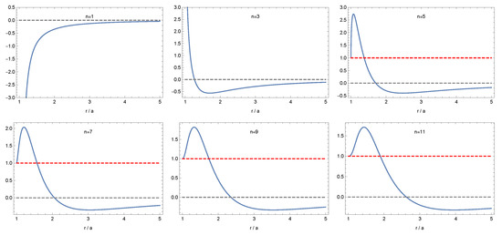
Figure 1. Plots of the NEC for several values of n. Here, the y-axis depicts $8\pi r^2(\rho +p_{\perp })$, plotting against $r/a$ on the x-axis. Of particular interest are the qualitative differences in behavior as $r/a\to 1$; we see divergent behavior for the $n=1$ and $n=3$ cases, whilst, for $n\ge 5$, we see $8\pi r^2(\rho +p_{\perp })\to 1$ as $r\to a$. This is ultimately due to the fact that the $n\ge 5$ cases are curvature regular, with globally finite stress-energy components.

5.2. Weak Energy Condition

In order to satisfy the weak energy condition (WEC), we require the NEC be satisfied, and in addition $\rho \ge 0$. But, in view of the asymptotic estimate (50) for $\rho$, we see that the WEC is always violated at large distances. Furthermore, it can be seen from Table 1 that the region in which the NEC is satisfied is always larger than that in which $\rho$ is positive (this would be as good as impossible to prove analytically for general n). Thus, we can conclude (see Table 2) that the WEC is satisfied for smaller regions than the NEC for all values of n.

Table 1. Regions of the spacetime where the orthonormal components of the stress-energy tensor satisfy certain inequalities.

n	$\mathit{\rho }+{\mathit{p}}_{\perp }\ge 0$	$\mathit{\rho }\ge 0$	${\mathit{p}}_{\perp }\ge 0$	$\mathit{\rho }-{\mathit{p}}_{\perp }\ge 0$
0	$a<r<\infty$	$a<r<\infty$	$a<r<\infty$	$a<r<\infty$
1	globally violated	globally violated	globally violated	globally violated
3	$a<r⪅1.26595a$	$a<r⪅1.07457a$	$a<r⪅1.41421a$	globally violated
5	$a<r⪅1.70468a$	$a<r⪅1.37005a$	$a<r\le 2a$	$a<r⪅1.00961a$
7	$a<r⪅2.05561a$	$a<r⪅1.62933a$	$a<r⪅2.44949a$	$a<r⪅1.11129a$
9	$a<r⪅2.35559a$	$a<r⪅1.85537a$	$a<r⪅2.82843$	$a<r⪅1.23076a$
11	$a<r⪅2.62173a$	$a<r⪅2.05757a$	$a<r⪅3.16228a$	$a<r⪅1.34552a$
⋮	⋮	⋮	⋮	⋮

Table 2. Regions of the spacetime where the energy conditions are satisfied.

n	NEC	WEC	SEC	DEC
0	$a<r<\infty$	$a<r<\infty$	$a<r<\infty$	$a<r<\infty$
1	globally violated	globally violated	globally violated	globally violated
3	$a<r⪅1.26595a$	$a<r⪅1.07457a$	same as NEC	globally violated
5	$a<r⪅1.70468a$	$a<r⪅1.37005a$	same as NEC	$a<r⪅1.00961a$
7	$a<r⪅2.05561a$	$a<r⪅1.62933a$	same as NEC	$a<r⪅1.11129a$
9	$a<r⪅2.35559a$	$a<r⪅1.85537a$	same as NEC	$a<r⪅1.23076a$
11	$a<r⪅2.62173a$	$a<r⪅2.05757a$	same as NEC	$a<r⪅1.34552a$
⋮	⋮	⋮	⋮	⋮

5.3. Strong Energy Condition

In order to satisfy the strong energy condition (SEC), we require the NEC to be satisfied, and in addition $\rho +p_r+2p_{\perp }=2p_{\perp }\ge 0$. But regardless of whether one is above or below the horizon, the second of these conditions $p_{\perp }\ge 0$ amounts to

$$\begin{array}{c}\hfill 0<a<r\le a\sqrt{n-1}.\end{array}$$

(57)

However, it can be seen from Table 1 that the region in which the NEC is satisfied is always smaller than that in which $p_{\perp }$ is positive (this would be as good as impossible to prove analytically for general n). Thus, we can conclude (see Table 2) that the SEC is satisfied in the same region as the NEC for all values of n.

5.4. Dominant Energy Condition

The dominant energy condition is the strongest of the standard classical energy conditions. Perhaps the best physical interpretation of the DEC is that, for any observer with timelike 4-velocity $V^a$, the flux vector $F^a=T^{ab}{V}_b$ is non-spacelike (timelike or null). It is a standard result that, in spherical symmetry (in fact, for any type I stress-energy tensor), this reduces to positivity of the energy density $\rho >0$ combined with the condition $|p_i|\le \rho$. Since, in the current framework, for the radial pressure, we always have $p_r=-\rho$, the only real constraint comes from demanding $|p_{\perp }|\le \rho$. But this means we want both $\rho +p_{\perp }\ge 0$ and $\rho -p_{\perp }\ge 0$. The first of these conditions is just the NEC, so the only new constraint comes from the second condition. By inspection, it can be seen from Table 1 that the region in which the NEC is satisfied is always larger than that in which $\rho -p_{\perp }$ is positive (this would be as good as impossible to prove analytically for general n). Thus, we can conclude (see Table 2) that the DEC is satisfied for smaller regions than the NEC for all values of n.

6. ISCO and Photon Sphere Analysis

It should be noted that particle orbits around quantum-corrected Schwarzschild black holes have previously been explored in Reference [91], for the case of timelike test particles, and in Reference [92], for a treatment of the photon ring. For ease of exposition, we feel it is worthwhile presenting a unified pedagogical derivation of the locations of the orbits of interest via the following discussion.

We have the generalized quantum modified Schwarzschild metric

$$\begin{array}{ccc}\hfill \mathrm{d}{s}^2& =& -\left\{{\left(1-\frac{a^2}{r^2}\right)}^{\frac{n}{2}}-\frac{2m}{r}\right\}\mathrm{d}{t}^2+\frac{\mathrm{d}{r}^2}{{\left(1-\frac{a^2}{r^2}\right)}^{\frac{n}{2}}-\frac{2m}{r}}+r^2\mathrm{d}{\Omega }_2^2.\hfill \end{array}$$

(58)

Let us now find the location of both the photon sphere for massless particles, and the ISCO for massive particles, as functions of the parameters m, n, and a. Consider the tangent vector to the worldline of a massive or massless particle, parameterized by some arbitrary affine parameter, $\lambda$:

$$\begin{array}{c}\hfill g_{ab}\frac{\mathrm{d}{x}^a}{\mathrm{d}\lambda }\frac{\mathrm{d}{x}^b}{\mathrm{d}\lambda }=-g_{tt}{\left(\frac{\mathrm{d}t}{\mathrm{d}\lambda }\right)}^2+g_{rr}{\left(\frac{\mathrm{d}r}{\mathrm{d}\lambda }\right)}^2+r^2\left\{{\left(\frac{\mathrm{d}\theta }{\mathrm{d}\lambda }\right)}^2+{sin}^2\theta {\left(\frac{\mathrm{d}\varphi }{\mathrm{d}\lambda }\right)}^2\right\}.\end{array}$$

(59)

We may, without loss of generality, separate the two physically interesting cases (timelike and null) by defining:

$$\begin{array}{c}\hfill ϵ=\left\{\begin{array}{cc}\hfill -1& \mathrm{m}\mathrm{a}\mathrm{s}\mathrm{s}\mathrm{i}\mathrm{v}\mathrm{e}\mathrm{p}\mathrm{a}\mathrm{r}\mathrm{t}\mathrm{i}\mathrm{c}\mathrm{l}\mathrm{e},\mathrm{i}.\mathrm{e}.,\mathrm{t}\mathrm{i}\mathrm{m}\mathrm{e}\mathrm{l}\mathrm{i}\mathrm{k}\mathrm{e}\mathrm{w}\mathrm{o}\mathrm{r}\mathrm{l}\mathrm{d}\mathrm{l}\mathrm{i}\mathrm{n}\mathrm{e}\hfill \\ \hfill 0& \mathrm{m}\mathrm{a}\mathrm{s}\mathrm{s}\mathrm{l}\mathrm{e}\mathrm{s}\mathrm{s}\mathrm{p}\mathrm{a}\mathrm{r}\mathrm{t}\mathrm{i}\mathrm{c}\mathrm{l}\mathrm{e},\mathrm{i}.\mathrm{e}.,\mathrm{n}\mathrm{u}\mathrm{l}\mathrm{l}\mathrm{w}\mathrm{o}\mathrm{r}\mathrm{l}\mathrm{d}\mathrm{l}\mathrm{i}\mathrm{n}\mathrm{e}.\hfill \end{array}\right.\end{array}$$

(60)

That is, $\mathrm{d}{s}^2/\mathrm{d}{\lambda }^2=ϵ$. Due to the metric being spherically symmetric, we may fix $\theta =\frac{\pi }{2}$ arbitrarily and view the reduced equatorial problem:

$$\begin{array}{c}\hfill g_{ab}\frac{\mathrm{d}{x}^a}{\mathrm{d}\lambda }\frac{\mathrm{d}{x}^b}{\mathrm{d}\lambda }=-g_{tt}{\left(\frac{\mathrm{d}t}{\mathrm{d}\lambda }\right)}^2+g_{rr}{\left(\frac{\mathrm{d}r}{\mathrm{d}\lambda }\right)}^2+r^2{\left(\frac{\mathrm{d}\varphi }{\mathrm{d}\lambda }\right)}^2=ϵ.\end{array}$$

(61)

The Killing symmetries yield the following expressions for the conserved energy E and angular momentum L per unit mass:

$$\begin{array}{c}\hfill \left\{{\left(1-\frac{a^2}{r^2}\right)}^{\frac{n}{2}}-\frac{2m}{r}\right\}\left(\frac{\mathrm{d}t}{\mathrm{d}\lambda }\right)=E;r^2\left(\frac{\mathrm{d}\varphi }{\mathrm{d}\lambda }\right)=L.\end{array}$$

(62)

Hence,

$$\begin{array}{c}\hfill {\left\{{\left(1-\frac{a^2}{r^2}\right)}^{\frac{n}{2}}-\frac{2m}{r}\right\}}^{-1}\left\{-E^2+{\left(\frac{\mathrm{d}r}{\mathrm{d}\lambda }\right)}^2\right\}+\frac{L^2}{r^2}=ϵ,\end{array}$$

(63)

implying

$$\begin{array}{c}\hfill {\left(\frac{\mathrm{d}r}{\mathrm{d}\lambda }\right)}^2=E^2+\left\{{\left(1-\frac{a^2}{r^2}\right)}^{\frac{n}{2}}-\frac{2m}{r}\right\}\left\{ϵ-\frac{L^2}{r^2}\right\}.\end{array}$$

(64)

This gives “effective potentials" for geodesic orbits as follows:

$$\begin{array}{c}\hfill V_{ϵ}\left(r\right)=\left\{{\left(1-\frac{a^2}{r^2}\right)}^{\frac{n}{2}}-\frac{2m}{r}\right\}\left\{-ϵ+\frac{L^2}{r^2}\right\}.\end{array}$$

(65)

6.1. Photon Orbits

For a photon orbit, we have the massless particle case $ϵ=0$. Since we are in a spherically symmetric environment, solving for the locations of such orbits amounts to finding the coordinate location of the “photon sphere”. These circular orbits occur at $V_0^{{}^{\prime }}\left(r\right)=0$. That is:

$$\begin{array}{c}\hfill V_0\left(r\right)=\left\{{\left(1-\frac{a^2}{r^2}\right)}^{\frac{n}{2}}-\frac{2m}{r}\right\}\left\{\frac{L^2}{r^2}\right\},\end{array}$$

(66)

leading to:

$$\begin{array}{c}\hfill V_0^{{}^{\prime }}\left(r\right)=\frac{L^2}{r^4}\left\{6m+r{\left(1-\frac{a^2}{r^2}\right)}^{\frac{n}{2}-1}\left[(n+2)\frac{a^2}{r^2}-2\right]\right\}.\end{array}$$

(67)

Solving $V_0^{{}^{\prime }}\left(r\right)=0$ analytically is intractable, but we may perform a Taylor series expansion of the above function about $a=0$ for a valid approximation (recall a is associated with the Planck length).

To fifth-order, this yields:

$$\begin{array}{c}\hfill V_0^{{}^{\prime }}\left(r\right)=\frac{2L^2}{r^4}(3m-r)+\frac{2L^{2}n{a}^2}{r^5}-\frac{3n{a}^4{L}^2(n-2)}{4r^7}+\mathcal{O}\left(L^2{a}^6/r^9\right).\end{array}$$

(68)

Equating this to zero and solving for r yields:

$$\begin{array}{c}\hfill r_{\gamma }=3m\left\{1+\frac{a^{2}n}{{\left(3m\right)}^2}-\frac{n(11n-6)a^4}{8{\left(3m\right)}^4}+\mathcal{O}(a^6/m^6)\right\}.\end{array}$$

(69)

The $a=0$, (or $n=0$), Schwarzschild sanity check reproduces $r_{\gamma }=3m$, the expected result.

To verify stability, we check the sign of $V_0^{{}^{″}}\left(r\right)$:

$$\begin{array}{c}\hfill V_0^{{}^{″}}\left(r\right)=-\frac{L^2}{r^4}\left\{\frac{24m}{r}-{\left(1-\frac{a^2}{r^2}\right)}^{\frac{n}{2}-2}\left[6-(7n+12)\frac{a^2}{r^2}+(n+2)(n+3)\frac{a^4}{r^4}\right]\right\}.\end{array}$$

(70)

We now substitute the approximate expression for $r_{\gamma }$ into Equation (70) to determine the sign of $V_0^{″}\left(r_{\gamma }\right)$. We find:

$$\begin{array}{c}\hfill V_0^{″}\left(r_{\gamma }\right)=-\frac{2L^2}{81m^4}\left\{1-\frac{3n{a}^2}{{\left(3m\right)}^2}+\frac{n(67n-6)a^4}{8{\left(3m\right)}^4}+\mathcal{O}(a^6/m^6)\right\}.\end{array}$$

(71)

Given that all bracketed terms to the right of the 1 are strictly subdominant in view of $a\ll m$, we may conclude that $V_0^{{}^{″}}\left(r_{\gamma }\right)<0$, and, hence, the null orbits at $r=r_{\gamma }$ are unstable.

Let us now recall the generalized form of Equation (66), and specialize to $n=5$ (the lowest value for n for which our quantum deformed Schwarzschild spacetime is regular). We have:

$$\begin{array}{ccc}\hfill V_0(r,n=5)& =& \frac{L^2}{r^2}\left\{{\left(1-\frac{a^2}{r^2}\right)}^{\frac{5}{2}}-\frac{2m}{r}\right\};\hfill \\ & & \hfill \end{array}$$

(72)

$$\begin{array}{ccc}\hfill V_0^{\prime }(r,n=5)& =& \frac{L^2}{r^4}\left\{6m-\sqrt{r^2-a^2}\left(2-\frac{9a^2}{r^2}+\frac{7a^4}{r^4}\right)\right\}.\hfill \end{array}$$

(73)

Once again, setting this to zero and attempting to solve analytically is an intractable line of inquiry, and we instead inflict Taylor series expansions about $a=0$.

To fifth-order, we have the following:

$$\begin{array}{l}{V}_0^{\prime }(r,n=5)=-\frac{2L^2}{r^3}\left\{1-\frac{3m}{r}-\frac{5a^2}{r^2}+\frac{45L^2{a}^4}{8r^4}+\mathcal{O}(a^6/r^6)\right\};\\ ⟹r_{\gamma }=3m\left\{1+\frac{5a^2}{{\left(3m\right)}^2}-\frac{245a^4}{8{\left(3m\right)}^4}+\mathcal{O}(a^6/m^6)\right\},\end{array}$$

(74)

which is consistent with the result for general n displayed in Equation (69).

6.2. ISCOs

For massive particles, the geodesic orbit corresponds to a timelike worldline, and we have the case that $ϵ=-1$. Therefore:

$$\begin{array}{c}\hfill V_{-1}\left(r\right)=\left\{{\left(1-\frac{a^2}{r^2}\right)}^{\frac{n}{2}}-\frac{2m}{r}\right\}\left\{1+\frac{L^2}{r^2}\right\},\end{array}$$

(75)

and it is easily verified that this leads to:

$$\begin{array}{c}\hfill V_{-1}^{{}^{\prime }}\left(r\right)=\frac{2m(3L^2+r^2)}{r^4}+\frac{{(1-a^2/r^2)}^{\frac{n}{2}-1}}{r^3}\left[n{a}^2+L^2\left((n+2)\frac{a^2}{r^2}-2\right)\right].\end{array}$$

(76)

For small a, we have

$$\begin{array}{c}\hfill V_{-1}\left(r\right)=\left\{1+\frac{L^2}{r^2}\right\}\left\{1-\frac{2m}{r}-\frac{n{a}^2}{2r^2}+\frac{n(n-2)a^4}{8r^4}+\mathcal{O}\left(\frac{a^6}{r^6}\right)\right\},\end{array}$$

(77)

and

$$\begin{array}{c}\hfill V_{-1}^{{}^{\prime }}\left(r\right)=\frac{2(L^2(3m-r)+m{r}^2)}{r^4}+\frac{(2L^2+r^2)n{a}^2}{r^5}-\frac{(3L^2+2r^2)n(n-2)a^4}{4r^7}+\mathcal{O}\left(\frac{a^6}{r^7}\right).\end{array}$$

(78)

Equating this to zero and rearranging for r presents an intractable line of inquiry. Instead, it is preferable to assume a fixed circular orbit at some $r=r_c$, and rearrange the required angular momentum $L_c$ to be a function of $r_c$, m, and a. It then follows that the innermost circular orbit shall be the value of $r_c$ for which $L_c$ is minimized. It is of course completely equivalent to perform this procedure for the mathematical object $L_c^2$, and we do so for tractability.

Hence, if $V_{-1}^{{}^{\prime }}\left(r_c\right)=0$, we have:

$$\begin{array}{c}\hfill L_c^2=\frac{n{a}^2{\left(1-\frac{a^2}{r^2}\right)}^{\frac{n}{2}}+2mr\left(1-\frac{a^2}{r^2}\right)}{{\left(1-\frac{a^2}{r^2}\right)}^{\frac{n}{2}}\left[2-(n+2)\frac{a^2}{r^2}\right]-\frac{6m}{r}\left(1-\frac{a^2}{r^2}\right)}.\end{array}$$

(79)

For small a, we have

$$\begin{array}{c}\hfill L_c^2=\frac{m{r}^2}{r-3m}+\frac{nr(r-m)a^2}{2{(r-3m)}^2}-\frac{n\{(2n+4)r^2+(5n-18)mr-9(n-2)m^2\}{a}^4}{8r{(r-3m)}^3}+\mathcal{O}\left(a^6\right).\end{array}$$

(80)

As a consistency check, for large $r_c$ (i.e., $r_c\gg a,m$), we observe from the dominant term of Equation (80) that $L_c\approx \sqrt{m{r}_c}$, which is consistent with the expected value when considering circular orbits in weak-field GR. Indeed, it is easy to check that, for large r, we have $L_c^2=m{r}_c+\mathcal{O}\left(1\right)$. Note that, in classical physics, the angular momentum per unit mass for a particle with angular velocity $\omega$ is $L_c\sim \omega r_c^2$. Kepler’s third law of planetary motion implies that $r_c^2{\omega }^2\sim G_{N}m/r_c$. (Here, m is the mass of the central object, as above.) It, therefore, follows that $L_c\sim \sqrt{G_{N}m/r_c}{r}_c$. That is $L_c\sim \sqrt{m{r}_c}$, as above.

Differentiating Equation (79) and finding the resulting roots is not analytically feasible. We instead differentiate Equation (80), obtaining a Taylor series for $\frac{\partial L_c^2}{\partial r_c}$ for small a:

$$\begin{array}{ccc}\frac{\partial L_c^2}{\partial r_c}\hfill & =\hfill & \frac{m{r}_c(r_c-6m)}{{(r_c-3m)}^2}-\frac{mn(5r_c-3m)a^2}{2{(r_c-3m)}^3}\hfill \\ \hfill & \hfill & -\frac{n\{16r_c^3+(n-2)(4r_c^3+21m{r}_c^2-36m^2{r}_c+27m^3)\}{a}^4}{8r_c^2{(r_c-3m)}^4}+\mathcal{O}\left(a^6\right).\hfill \end{array}$$

(81)

Solving for the stationary points yields:

$$\begin{array}{c}\hfill r_{\mathrm{ISCO}}=6m\left\{1+\frac{n{a}^2}{8m^2}-\frac{n(49n-22)a^4}{3456m^4}+\mathcal{O}\left(\frac{a^6}{m^6}\right)\right\},\end{array}$$

(82)

and the $a=0$ Schwarzschild sanity check reproduces $r_c=6m$ as required.

6.3. Summary

Denoting $r_{\mathrm{H}}$ as the location of the horizon, $r_{\gamma }$ as the location of the photon sphere, and $r_{\mathrm{ISCO}}$ as the location of the ISCO, we have the following summary:

• $r_H=2m\times \{1+\frac{n{a}^2}{2{\left(2m\right)}^2}-\frac{n(3n-2)a^4}{8{\left(2m\right)}^4}+\mathcal{O}\left(\frac{a^6}{m^6}\right)\}$;
• $r_{\gamma }=3m\times \left\{1+\frac{n{a}^2}{{\left(3m\right)}^2}-\frac{n(11n-6)a^4}{8{\left(3m\right)}^4}+\mathcal{O}\left(\frac{a^6}{m^6}\right)\right\}$;
• $r_{\mathrm{ISCO}}=6m\times \left\{1+\frac{n{a}^2}{8m^2}-\frac{n(49n-22)a^4}{3456m^4}+\mathcal{O}\left(\frac{a^6}{m^6}\right)\right\}$.

7. Regge–Wheeler Analysis

Now, considering the Regge–Wheeler equation, in view of the unified formalism developed in Reference [93] (also see References [64,94,95]), we may explicitly evaluate the Regge–Wheeler potentials for particles of spin $S\in \{0,1\}$ in our spacetime. Firstly, define a tortoise coordinate as follows:

$$\begin{array}{c}\hfill \mathrm{d}{r}_{\ast }=\frac{\mathrm{d}r}{{\left(1-\frac{a^2}{r^2}\right)}^{\frac{n}{2}}-\frac{2m}{r}}.\end{array}$$

(83)

This tortoise coordinate is, for general n, not analytically defined. However, let us make the coordinate transformation regardless; this yields the following expression for the metric:

$$\begin{array}{c}\hfill \mathrm{d}{s}^2=\left\{{\left(1-\frac{a^2}{r^2}\right)}^{\frac{n}{2}}-\frac{2m}{r}\right\}\left\{-\mathrm{d}{t}^2+\mathrm{d}{r}_{\ast }^2\right\}+r^2\left(\mathrm{d}{\theta }^2+{sin}^2\theta \mathrm{d}{\varphi }^2\right).\end{array}$$

(84)

It is convenient to write this as:

$$\begin{array}{c}\hfill \mathrm{d}{s}^2=A{\left(r_{\ast }\right)}^2\left\{-\mathrm{d}{t}^2+\mathrm{d}{r}_{\ast }^2\right\}+B{\left(r_{\ast }\right)}^2\left(\mathrm{d}{\theta }^2+{sin}^2\theta \mathrm{d}{\varphi }^2\right).\end{array}$$

(85)

The Regge–Wheeler equation is [93,94,95]:

$$\begin{array}{c}\hfill {\partial }_{r_{\ast }}^2\widehat{\varphi }+\{{\omega }^2-{\mathcal{V}}_S\}\widehat{\varphi }=0,\end{array}$$

(86)

where $\widehat{\varphi }$ is the scalar or vector field, $\mathcal{V}$ is the spin-dependent Regge–Wheeler potential for our particle, and $\omega$ is some temporal frequency component in the Fourier domain. For a scalar field ($S=0$), examination of the d’Alembertian equation quickly yields:

$$\begin{array}{c}\hfill {\mathcal{V}}_{S=0}=\left\{\frac{A^2}{B^2}\right\}\ell (\ell +1)+\frac{{\partial }_{r_{\ast }}^{2}B}{B}.\end{array}$$

(87)

For a massless vector field, ($S=1$, e.g., photon), explicit conformal invariance in 3+1 dimensions guarantees that the Regge–Wheeler potential can depend only on the ratio $A/B$, whence normalizing to known results implies:

$$\begin{array}{c}\hfill {\mathcal{V}}_{S=1}=\left\{\frac{A^2}{B^2}\right\}\ell (\ell +1).\end{array}$$

(88)

Collecting results, for $S\in \{0,1\}$, we have:

$$\begin{array}{c}\hfill {\mathcal{V}}_{S\in \{0,1\}}=\left\{\frac{A^2}{B^2}\right\}\ell (\ell +1)+(1-S)\frac{{\partial }_{r_{\ast }}^{2}B}{B}.\end{array}$$

(89)

The spin 2 axial mode is somewhat messier and (for current purposes) not of immediate interest. Note that, for our metric,

$$\begin{array}{c}\hfill {\partial }_{r_{\ast }}=\left\{{\left(1-\frac{a^2}{r^2}\right)}^{\frac{n}{2}}-\frac{2m}{r}\right\}{\partial }_r,\end{array}$$

(90)

and $B\left(r\right)=r$. We have:

$$\begin{array}{ccc}\frac{{\partial }_{r_{\ast }}^{2}B}{B}\hfill & =\hfill & \frac{{\partial }_{r_{\ast }}\left\{{\left(1-\frac{a^2}{r^2}\right)}^{\frac{n}{2}}-\frac{2m}{r}\right\}}{r}\hfill \\ \hfill & =\hfill & \frac{1}{r^2}\left\{{\left(1-\frac{a^2}{r^2}\right)}^{\frac{n}{2}}-\frac{2m}{r}\right\}\left\{n{\left(1-\frac{a^2}{r^2}\right)}^{\frac{n}{2}-1}\frac{a^2}{r^2}+\frac{2m}{r}\right\}.\hfill \end{array}$$

(91)

For small a:

$$\begin{array}{c}\hfill \frac{{\partial }_{r_{\ast }}^{2}B}{B}=\frac{2m(1-2m/r)}{r^3}+\frac{n(r-3m)}{r^5}{a}^2+\frac{n\left\{5\right(n-2)m-4(n-1\left)r\right\}}{4r^7}{a}^4+\mathcal{O}\left(\frac{m{a}^6}{r^9}\right).\end{array}$$

(92)

Therefore:

$$\begin{array}{ccc}\hfill {\mathcal{V}}_{S\in \{0,1\}}& =& \frac{1}{r^2}\left[{\left(1-\frac{a^2}{r^2}\right)}^{\frac{n}{2}}-\frac{2m}{r}\right]\left\{\ell \left(\ell +1\right)+\left(1-S\right)\left[n{\left(1-\frac{a^2}{r^2}\right)}^{\frac{n}{2}-1}\frac{a^2}{r^2}+\frac{2m}{r}\right]\right\}.\hfill \end{array}$$

(93)

This has the correct behavior as $a\to 0$, reducing to the Regge–Wheeler potential for Schwarzschild:

$$\begin{array}{c}\hfill \underset{a\to 0}{lim}{\mathcal{V}}_{S\in \{0,1\}}=\frac{1}{r^2}\left[1-\frac{2m}{r}\right]\left\{\ell (\ell +1)+(1-S)\frac{2m}{r}\right\}.\end{array}$$

(94)

In the small a approximation, we have the asymptotic result

$$\begin{array}{cc}{\mathcal{V}}_{S\in \{0,1\}}=& \frac{\left(1-\frac{2m}{r}\right)}{r^2}\left\{\ell (\ell +1)+(1-S)\frac{2m}{r}\right\}-\frac{n{a}^2}{2r^4}\left\{\ell (\ell +1)+2(1-S)\left[\frac{3m}{r}-1\right]\right\}\\ & +\frac{n{a}^4}{2r^6}\left\{\frac{(n-2)}{4}\left[\ell (\ell +1)\right]-\left(1-S\right)\left[2(n-1)+5\left(1-\frac{n}{2}\right)\frac{m}{r}\right]\right\}+\mathcal{O}\left(\frac{a^6}{r^8}\right).\end{array}$$

(95)

The Regge–Wheeler equation is fundamental to exploring the quasi-normal modes of the candidate spacetimes, an integral part of the “ringdown” phase of the LIGO calculation to detect astrophysical phenomena via gravitational waves. Explorations of the quasi-normal modes of various quantum-corrected black hole spacetimes have been performed in References [96,97,98,99,100].

8. Discussion and Conclusions

The original Kazakov–Solodukhin “quantum deformed Schwarzschild spacetime” [1] is certainly more “regular” than Schwarzschild spacetime, but it is not “regular” in the sense normally intended in the general relativity community. While the metric components are regular, both Christoffel symbols and curvature invariants diverge at the “center” of the spacetime, a 2-sphere where $r\to a$ with finite area $A=4\pi a^2$. The “smearing out” of the “center” to $r\to a$ is not sufficient to guarantee curvature regularity.

We have generalized the original Kazakov–Solodukhin spacetime to a two-parameter class compatible with the ideas mooted in Reference [1]. Our generalized two-parameter class of “quantum corrected” Schwarzschild spacetimes contains exemplars which have much better regularity properties, and we can distinguish three levels of regularity: metric regularity, Christoffel regularity, and regularity of the curvature invariants.

Furthermore, our generalized two-parameter class of models distorts Schwarzschild spacetime in a clear and controlled way—so providing yet more examples of black-hole “mimickers” potentially of interest for observational purposes. In this regard, we have analyzed the geometry, surface gravity, stress-energy, and classical energy conditions. We have also perturbatively analyzed the locations of ISCOs and photon spheres, and set up the appropriate Regge–Wheeler formalism for spin-1 and spin-0 excitations.

Overall, the general topic of “quantum corrected” Schwarzschild spacetimes is certainly of significant interest, and we hope that these specific examples may serve to encourage further investigation in this field.

References

- Kazakov, D.; Solodukhin, S. On quantum deformation of the Schwarzschild solution. Nucl. Phys. B 1994, 429, 153–176. [Google Scholar] [CrossRef]
- Solodukhin, S.N. “Nongeometric” contribution to the entropy of a black hole due to quantum corrections. Phys. Rev. D 1995, 51, 618–621. [Google Scholar] [CrossRef]
- Solodukhin, S.N. Two-dimensional quantum-corrected eternal black hole. Phys. Rev. D 1996, 53, 824–835. [Google Scholar] [CrossRef]
- Ashtekar, A.; Olmedo, J.; Singh, P. Quantum extension of the Kruskal spacetime. Phys. Rev. D 2018, 98, 126003. [Google Scholar] [CrossRef]
- Nojiri, S.; Odintsov, S.D. Can quantum-corrected btz black hole anti-evaporate? Mod. Phys. Lett. A 1998, 13, 2695–2704. [Google Scholar] [CrossRef]
- Maluf, R.V.; Neves, J. Bardeen regular black hole as a quantum-corrected Schwarzschild black hole. Int. J. Mod. Phys. D 2019, 28, 1950048. [Google Scholar] [CrossRef]
- Zaslavskii, O.B. Near-extremal and extremal quantum-corrected two-dimensional charged black holes. Class. Quantum Gravity 2004, 21, 2687–2701. [Google Scholar] [CrossRef]
- Ali, A.F.; Khalil, M.M. Black hole with quantum potential. Nucl. Phys. B 2016, 909, 173–185. [Google Scholar] [CrossRef]
- Calmet, X.; El-Menoufi, B.K. Quantum corrections to Schwarzschild black hole. Eur. Phys. J. C 2017, 77, 243. [Google Scholar] [CrossRef]
- Shahjalal, M. Shahjalal Phase transition of quantum-corrected Schwarzschild black hole in rainbow gravity. Phys. Lett. B 2018, 784, 6–11. [Google Scholar] [CrossRef]
- Qi, D.-J.; Liu, L.; Liu, S.-X. Quantum tunneling and remnant from a quantum-modified Schwarzschild space–time close to Planck scale. Can. J. Phys. 2019, 97, 1012–1018. [Google Scholar] [CrossRef]
- Shahjalal, M. Thermodynamics of quantum-corrected Schwarzschild black hole surrounded by quintessence. Nucl. Phys. B 2019, 940, 63–77. [Google Scholar] [CrossRef]
- Eslamzadeh, S.; Nozari, K. Tunneling of massless and massive particles from a quantum deformed Schwarzschild black hole surrounded by quintessence. Nucl. Phys. B 2020, 959, 115136. [Google Scholar] [CrossRef]
- Good, M.R.; Linder, E.V. Schwarzschild Metric with Planck Length. arXiv 2020, arXiv:2003.01333. [Google Scholar]
- Nozari, K.; Hajebrahimi, M. Geodesic Structure of the Quantum-Corrected Schwarzschild Black Hole Surrounded by Quintessence. arXiv 2020, arXiv:2004.14775. [Google Scholar]
- Nozari, K.; Hajebrahimi, M.; Saghafi, S. Quantum corrections to the accretion onto a Schwarzschild black hole in the background of quintessence. Eur. Phys. J. C 2020, 80, 1–13. [Google Scholar] [CrossRef]
- Burger, D.J.; Moynihan, N.; Das, S.; Haque, S.S.; Underwood, B. Towards the Raychaudhuri equation beyond general relativity. Phys. Rev. D 2018, 98, 024006. [Google Scholar] [CrossRef]
- Russo, J.G.; Tseytlin, A. Scalar-tensor quantum gravity in two dimensions. Nucl. Phys. B 1992, 382, 259–275. [Google Scholar] [CrossRef]
- Jacobson, T. When is gttgrr = −1? Class. Quantum Gravity 2007, 24, 5717–5719. [Google Scholar] [CrossRef]
- Kiselev, V.V. Quintessence and black holes. Class. Quantum Gravity 2003, 20, 1187–1197. [Google Scholar] [CrossRef]
- Visser, M. The Kiselev black hole is neither perfect fluid, nor is it quintessence. Class. Quantum Gravity 2019, 37, 045001. [Google Scholar] [CrossRef]
- Boonserm, P.; Ngampitipan, T.; Simpson, A.; Visser, M. Decomposition of the total stress energy for the generalized Kiselev black hole. Phys. Rev. D 2020, 101, 024022. [Google Scholar] [CrossRef]
- Bardeen, J.M. Non-singular general-relativistic gravitational collapse. In Proceedings of the GR5 Conference, Tbilisi, Georgia, 9–13 September 1968; p. 174. [Google Scholar]
- Roman, T.A.; Bergmann, P.G. Stellar collapse without singularities? Phys. Rev. D 1983, 28, 1265–1277. [Google Scholar] [CrossRef]
- Borde, A. Regular black holes and topology change. Phys. Rev. D 1997, 55, 7615–7617. [Google Scholar] [CrossRef]
- Bronnikov, K.A. Regular magnetic black holes and monopoles from nonlinear electrodynamics. Phys. Rev. D 2001, 63, 044005. [Google Scholar] [CrossRef]
- Moreno, C.; Sarbach, O. Stability properties of black holes in self-gravitating nonlinear electrodynamics. Phys. Rev. D 2003, 67, 024028. [Google Scholar] [CrossRef]
- Ayon-Beato, E.; Garcia, A. Four parameter regular black hole solution. Gen. Rel. Grav. 2005, 37, 635. [Google Scholar] [CrossRef]
- Hayward, S.A. Formation and Evaporation of Nonsingular Black Holes. Phys. Rev. Lett. 2006, 96, 031103. [Google Scholar] [CrossRef]
- Bronnikov, K.A.; Fabris, J.C. Regular Phantom Black Holes. Phys. Rev. Lett. 2006, 96, 251101. [Google Scholar] [CrossRef]
- Bronnikov, K.A.; Dehnen, H.; Melnikov, V.N. Regular black holes and black universes. Gen. Relativ. Gravit. 2007, 39, 973–987. [Google Scholar] [CrossRef]
- Lemos, J.P.S.; Zaslavskii, O.B. Quasi-black holes: Definition and general properties. Phys. Rev. D 2007, 76, 084030. [Google Scholar] [CrossRef]
- Ansoldi, S. Spherical black holes with regular center: A Review of existing models including a recent realization with Gaussian sources. arXiv 2008, arXiv:0802.0330. [Google Scholar]
- Lemos, J.P.S.; Zanchin, V.T. Regular black holes: Electrically charged solutions, Reissner-Nordström outside a de Sitter core. Phys. Rev. D 2011, 83, 124005. [Google Scholar] [CrossRef]
- Bronnikov, K.A.; Konoplya, R.A.; Zhidenko, A. Instabilities of wormholes and regular black holes supported by a phantom scalar field. Phys. Rev. D 2012, 86, 024028. [Google Scholar] [CrossRef]
- Bambi, C.; Modesto, L. Rotating regular black holes. Phys. Lett. B 2013, 721, 329–334. [Google Scholar] [CrossRef]
- Bardeen, J.M. Black hole evaporation without an event horizon. arXiv 2014, arXiv:1406.4098. [Google Scholar]
- Frolov, V.P. Information loss problem and a ‘black hole’ model with a closed apparent horizon. JHEP 2014, 5, 49. [Google Scholar] [CrossRef]
- Frolov, V.P. Do Black Holes Exist? arXiv 2014, arXiv:1411.6981. [Google Scholar]
- Balart, L.; Vagenas, E.C. Regular black holes with a nonlinear electrodynamics source. Phys. Rev. D 2014, 90, 124045. [Google Scholar] [CrossRef]
- De Lorenzo, T.; Pacilio, C.; Rovelli, C.; Speziale, S. On the effective metric of a Planck star. Gen. Relativ. Gravit. 2015, 47, 41. [Google Scholar] [CrossRef]
- Frolov, V.P. Notes on nonsingular models of black holes. Phys. Rev. D 2016, 94, 104056. [Google Scholar] [CrossRef]
- Fan, Z.-Y.; Wang, X. Construction of regular black holes in general relativity. Phys. Rev. D 2016, 94, 124027. [Google Scholar] [CrossRef]
- Frolov, V.P.; Zelnikov, A. Quantum radiation from an evaporating nonsingular black hole. Phys. Rev. D 2017, 95, 124028. [Google Scholar] [CrossRef]
- Frolov, V.P. Remarks on non-singular black holes. EPJ Web Conf. 2018, 168, 01001. [Google Scholar] [CrossRef]
- Cano, P.A.; Chimento, S.; Ortín, T.; Ruipérez, A. Regular stringy black holes? Phys. Rev. D 2019, 99. [Google Scholar] [CrossRef]
- Bardeen, J.M. Models for the nonsingular transition of an evaporating black hole into a white hole. arXiv 2018, arXiv:1811.06683. [Google Scholar]
- Carballo-Rubio, R.; Di Filippo, F.; Liberati, S.; Pacilio, C.; Visser, M. On the viability of regular black holes. J. High Energy Phys. 2018, 2018, 23. [Google Scholar] [CrossRef]
- Carballo-Rubio, R.; Di Filippo, F.; Liberati, S.; Visser, M. Phenomenological aspects of black holes beyond general relativity. Phys. Rev. D 2018, 98, 124009. [Google Scholar] [CrossRef]
- Carballo-Rubio, R.; Di Filippo, F.; Liberati, S.; Visser, M. Opening the Pandora’s box at the core of black holes. Class. Quantum Gravity 2020, 37, 145005. [Google Scholar] [CrossRef]
- Carballo-Rubio, R.; Di Filippo, F.; Liberati, S.; Visser, M. Geodesically complete black holes. Phys. Rev. D 2020, 101, 084047. [Google Scholar] [CrossRef]
- Carballo-Rubio, R.; Di Filippo, F.; Liberati, S.; Pacilio, C.; Visser, M. Inner horizon instability and the unstable cores of regular black holes. J. High Energy Phys. 2021, 2021, 1–16. [Google Scholar] [CrossRef]
- Cardoso, V.; Hopper, S.; Macedo, C.F.B.; Palenzuela, C.; Pani, P. Gravitational-wave signatures of exotic compact objects and of quantum corrections at the horizon scale. Phys. Rev. D 2016, 94, 084031. [Google Scholar] [CrossRef]
- Visser, M.; Barceló, C.; Liberati, S.; Sonego, S. Small, dark, and heavy: But is it a black hole? PoS 2009, 75, 10. [Google Scholar] [CrossRef]
- Visser, M. Black holes in general relativity. PoS 2009, 75. [Google Scholar] [CrossRef]
- Visser, M.; Wiltshire, D.L. Stable gravastars—An alternative to black holes? Class. Quantum Gravity 2004, 21, 1135–1151. [Google Scholar] [CrossRef]
- Barceló, C.; Liberati, S.; Sonego, S.; Visser, M. Black Stars, Not Holes. Sci. Am. 2009, 301, 38–45. [Google Scholar] [CrossRef] [PubMed]
- Simpson, A.; Visser, M. Black-bounce to traversable wormhole. J. Cosmol. Astropart. Phys. 2019, 2019, 042. [Google Scholar] [CrossRef]
- Simpson, A.; Martín-Moruno, P.; Visser, M. Vaidya spacetimes, black-bounces, and traversable wormholes. Class. Quantum Gravity 2019, 36, 145007. [Google Scholar] [CrossRef]
- Lobo, F.S.N.; Simpson, A.; Visser, M. Dynamic thin-shell black-bounce traversable wormholes. Phys. Rev. D 2020, 101, 124035. [Google Scholar] [CrossRef]
- Simpson, A.; Visser, M. Regular Black Holes with Asymptotically Minkowski Cores. Universe 2019, 6, 8. [Google Scholar] [CrossRef]
- Berry, T.; Lobo, F.S.N.; Simpson, A.; Visser, M. Thin-shell traversable wormhole crafted from a regular black hole with asymptotically Minkowski core. Phys. Rev. D 2020, 102, 064054. [Google Scholar] [CrossRef]
- Berry, T.; Simpson, A.; Visser, M. Photon Spheres, ISCOs, and OSCOs: Astrophysical Observables for Regular Black Holes with Asymptotically Minkowski Cores. Universe 2020, 7, 2. [Google Scholar] [CrossRef]
- Boonserm, P.; Ngampitipan, T.; Simpson, A.; Visser, M. Exponential metric represents a traversable wormhole. Phys. Rev. D 2018, 98, 084048. [Google Scholar] [CrossRef]
- Barausse, E.; Berti, E.; Hertog, T.; Hughes, S.A.; Jetzer, P.; Pani, P.; Sotiriou, T.P.; Tamanini, N.; Witek, H.; Yagi, K.; et al. Prospects for fundamental physics with LISA. Gen. Relativ. Gravit. 2020, 52, 1–33. [Google Scholar] [CrossRef]
- Visser, M. Physical observability of horizons. Phys. Rev. D 2014, 90, 127502. [Google Scholar] [CrossRef]
- Hawking, S.W. Information Preservation and Weather Forecasting for Black Holes. arxiv 2014, arXiv:1401.5761. [Google Scholar]
- Lobo, F.S.N.; Rodrigues, M.E.; Silva, M.V.D.S.; Simpson, A.; Visser, M. Novel black-bounce geometries. arXiv 2021, arXiv:2009.12057. [Google Scholar]
- Visser, M. Dirty black holes: Thermodynamics and horizon structure. Phys. Rev. D 1992, 46, 2445–2451. [Google Scholar] [CrossRef]
- Available online: https://en.wikipedia.org/wiki/Energy_condition (accessed on 26 May 2021).
- Tipler, F.J. Energy conditions and spacetime singularities. Phys. Rev. D 1978, 17, 2521–2528. [Google Scholar] [CrossRef]
- Borde, A. Geodesic focusing, energy conditions and singularities. Class. Quantum Gravity 1987, 4, 343–356. [Google Scholar] [CrossRef]
- Klinkhammer, G. Averaged energy conditions for free scalar fields in flat spacetime. Phys. Rev. D 1991, 43, 2542–2548. [Google Scholar] [CrossRef]
- Ford, L.H.; Roman, T.A. Averaged energy conditions and quantum inequalities. Phys. Rev. D 1995, 51, 4277–4286. [Google Scholar] [CrossRef]
- Visser, M. Lorentzian Wormholes: From Einstein to Hawking; Springer: New York, NY, USA, 1995. [Google Scholar]
- Fewster, C.J.; Roman, T.A. Null energy conditions in quantum field theory. Phys. Rev. D 2003, 67, 044003. [Google Scholar] [CrossRef]
- Barceló, C.; Visser, M. Twilight for the energy conditions? Int. J. Mod. Phys. D 2002, 11, 1553–1560. [Google Scholar] [CrossRef]
- Visser, M. Energy Conditions in the Epoch of Galaxy Formation. Science 1997, 276, 88–90. [Google Scholar] [CrossRef] [PubMed]
- Visser, M.; Barceló, C. Energy conditions and their cosmological implications. arXiv 1999, arXiv:gr-qc/0001099. [Google Scholar]
- Visser, M. Gravitational vacuum polarization. II. Energy conditions in the Boulware vacuum. Phys. Rev. D 1996, 54, 5116–5122. [Google Scholar] [CrossRef] [PubMed]
- Roman, T.A. Some thoughts on energy conditions and wormholes. arXiv 2004, arXiv:gr-qc/0409090. [Google Scholar]
- Cattoen, C.; Visser, M. Cosmological milestones and energy conditions. J. Phys. Conf. Ser. 2007, 68, 012011. [Google Scholar] [CrossRef]
- Visser, M. Energy conditions and galaxy formation. arXiv 1997, arXiv:gr-qc/9710010. [Google Scholar] [CrossRef]
- Fewster, C.J.; Galloway, G.J. Singularity theorems from weakened energy conditions. Class. Quantum Gravity 2011, 28, 125009. [Google Scholar] [CrossRef]
- Zaslavskii, O. Regular black holes and energy conditions. Phys. Lett. B 2010, 688, 278–280. [Google Scholar] [CrossRef]
- Martín-Moruno, P.; Visser, M. Classical and Semi-classical Energy Conditions. Black Hole Phys. 2017, 189, 193–213. [Google Scholar] [CrossRef]
- Martin-Moruno, P.; Visser, M. Semiclassical energy conditions for quantum vacuum states. J. High Energy Phys. 2013, 2013, 1–36. [Google Scholar] [CrossRef]
- Martín-Moruno, P.; Visser, M. Classical and quantum flux energy conditions for quantum vacuum states. Phys. Rev. D 2013, 88. [Google Scholar] [CrossRef]
- Curiel, E. A Primer on Energy Conditions. Einstein Stud. 2017, 13, 43–104. [Google Scholar] [CrossRef]
- Martín-Moruno, P.; Visser, M. Semi-classical and nonlinear energy conditions. In Proceedings of the 14th Marcel Grossmann Meeting, Rome, Italy, 12–18 July 2015. [Google Scholar] [CrossRef]
- Deng, X.-M. Geodesics and periodic orbits around quantum-corrected black holes. Phys. Dark Universe 2020, 30, 100629. [Google Scholar] [CrossRef]
- Peng, J.; Guo, M.; Feng, X.H. Influence of Quantum Correction on the Black Hole Shadows, Photon Rings and Lensing Rings. arXiv 2020, arXiv:2008.00657. [Google Scholar]
- Boonserm, P.; Ngampitipan, T.; Visser, M. Regge-Wheeler equation, linear stability, and greybody factors for dirty black holes. Phys. Rev. D 2013, 88. [Google Scholar] [CrossRef]
- Flachi, A.; Lemos, J.P.S. Quasinormal modes of regular black holes. Phys. Rev. D 2013, 87, 24034. [Google Scholar] [CrossRef]
- Fernando, S.; Correa, J. Quasinormal modes of the Bardeen black hole: Scalar perturbations. Phys. Rev. D 2012, 86. [Google Scholar] [CrossRef]
- Rincón, Á.; Panotopoulos, G. Quasinormal modes of an improved Schwarzschild black hole. Phys. Dark Universe 2020, 30, 100639. [Google Scholar] [CrossRef]
- Konoplya, R. Quantum corrected black holes: Quasinormal modes, scattering, shadows. Phys. Lett. B 2020, 804, 135363. [Google Scholar] [CrossRef]
- Saleh, M.; Bouetou, B.T.; Kofane, T.C. Quasinormal modes of a quantum-corrected Schwarzschild black hole: Gravitational and Dirac perturbations. Astrophys. Space Sci. 2016, 361, 1–8. [Google Scholar] [CrossRef]
- Zhang, Y.; Lu, X. Electromagnetic quasinormal mode of quantum corrected Schwarzschild black hole. J. Kunming Univ. Sci. Technol. Nat. Sci. Ed. 2016, 6, 139–144. [Google Scholar] [CrossRef]
- Saleh, M.; Thomas, B.B.; Kofané, T.C. Quasinormal modes of scalar perturbation around a quantum-corrected Schwarzschild black hole. Astrophys. Space Sci. 2014, 350, 721–726. [Google Scholar] [CrossRef]
Publisher’s Note: MDPI stays neutral with regard to jurisdictional claims in published maps and institutional affiliations. |
© 2021 by the authors. Licensee MDPI, Basel, Switzerland. This article is an open access article distributed under the terms and conditions of the Creative Commons Attribution (CC BY) license (https://creativecommons.org/licenses/by/4.0/).