Electron-Positron Vacuum Instability in Strong Electric Fields. Relativistic Semiclassical Approach

Abstract

The instability of electron-positron vacuum in strong electric fields is studied. First, falling to the Coulomb center is discussed at $Z>137/2$ for a spinless boson and at $Z>137$ for electron. Subsequently, focus is concentrated on description of deep electron levels and spontaneous positron production in the field of a finite-size nucleus with the charge $Z>Z_{\mathrm{cr}}\simeq 170$. Next, these effects are studied in application to the low-energy heavy-ion collisions. Subsequently, we consider phenomenon of “electron condensation” on levels of upper continuum crossed the boundary of the lower continuum $ϵ=-m$ in the field of a supercharged nucleus with $Z\gg Z_{\mathrm{cr}}$. Finally, attention is focused on many-particle problems of polarization of the quantum electrodynamics (QED) vacuum and electron condensation at ultra-short distances from a source of charge. We argue for a principal difference of cases, when the size of the source is larger than the pole size $r_{\mathrm{pole}}$, at which the dielectric permittivity of the vacuum reaches zero and smaller $r_{\mathrm{pole}}$. Some arguments are presented in favor of the logical consistency of QED. All of the problems are considered within the same relativistic semiclassical approach.

1. Introduction

I dedicate this review to the blessed memory of Vladimir Stepanovich Popov, who recently left us as the result of a many-year hard illness, which prevented him working actively in his last years. The problem of the electron-positron pair production when the ground-state electron level dives below the energy $-m{c}^2$ (m is the electron mass, c is the speed of light) was of his interest starting from the end of 1960-th. Especially he contributed to this problem during the 1970s. V. S. Popov was awarded the I. Y. Pomeranchuk Prize in 2019 for his outstanding contributions to the theory of ionization of atoms and ions in the field of intense laser radiation and the theory of the creation of electron-positron pairs in the presence of superstrong external fields.

We worked together with Vladimir Stepanovich on problems of supercritical atoms with the charge $Z>Z_{\mathrm{cr}}=170-173$ during 1976–1978 when we developed semiclassical treatment of this problem. These works, cf. [1,2,3,4,5,6,7] became a part of my PhD thesis [8] that was defended in 1977 under the guidance of Arkadi Benediktovich Migdal.

As follows from the Dirac equation in the Coulomb field of a point-like nucleus with $Z>1/e^2$ (in units $\hslash =c=1$, which will be used in this paper, $e^2\simeq 1/137$), the electron that occupied the ground-state level should fall to the center. Following the idea of I. Pomeranchuk and Ya. Smorodinsky [9], the solution of the problem of the falling of the electron to the center can be found while taking into account the fact that the real nuclei have a finite radius. With increasing Z, the energy of the ground state level decreases and, at $Z>Z_{cr}$, crosses the boundary of the lower continuum $ϵ=-m$. The problem received a new push in the end of the 1960sThe important role of the Pauli principle was emphasized in [10]. However the authors erroneously assumed delocalization of the electron state with $ϵ\simeq -m$. Independently, W. Pieper and W. Greiner [11] (in numerical analysis) and V. S. Popov [12,13,14,15,16] (in analytical and numerical studies) correctly evaluated the value of the critical charge to be $Z_{\mathrm{cr}}\simeq 169-173$, depending on assumptions regarding the charge distribution inside the nucleus and the ratio $Z/A$. It was argued that two positrons with the energies $>m$ go off to infinity and electrons with $ϵ<-m$ screen the field of the nucleus by the charge $-2e$. The typical distance characterizing electrons of the vacuum K shell is $\sim 1/\left(3m\right)\gg R_{\mathrm{nucl}}$, cf. [7]. Subsequently, there appeared an idea to observe positron production in heavy-ion collisions, where the supercritical atom is formed for a short time [17,18]. As the reviews of these problems, I can recommend [19,20,21].

In 1976, with the inauguration of the UNI-LAC accelerator in GSI, Darmstadt, it became possible to accelerate heavy ions up to uranium below and above the Coulomb barrier. Instead of a positron line that is associated with the spontaneous decay of the electron-positron vacuum, mysterious line structures were observed, which, in spite of many attempts, did not get a reasonable theoretical interpretation. The experimental results on the mentioned positron lines proved to be erroneous. New experiments were conducted during 1993–1995, cf. [22,23,24]. The presence of the line structures was not observed. Events, which could be interpreted as the effect of the decay of the QED vacuum with the spontaneous production of the electron-positron pair, were not selected. In spite of the effect of the spontaneous production of positrons in the electric field of the supercharged nucleus being predicted many decades ago, it has not yet been observed experimentally in heavy-ion collisions.

One also studied a possibility of a nuclear sticking in the process of the heavy-ion collisions [25,26]. Although these expectations did not find a support in further investigations, extra arguments were given for a possibility of the observation of the spontaneous positron production in the heavy-ion collisions, cf. [27]. Especially, the usage of transuranium ions looks very promising [28]. Besides a spontaneous production of positrons, a more intensive induced production of pairs occurs due to an excitation of nuclear levels, cf. [20]. Therefore, the key question is how to distinguish spontaneous production of positrons that originated in the decay of the electron-positron vacuum from the induced production and other competing processes.

New studies of low-energy heavy-ion collisions at the supercritical regime are anticipated at the upcoming accelerator facilities in Germany, Russia, and China [29,30,31]. This possibility renewed theoretical interest to the problem [27,32,33,34]. As one can see from the numerical results reported in [34], these results support those that were obtained in earlier works, although a comparison with the analytical results derived in [1,2,3,4,5,6,7] was not performed. Additionally, it should be noted that there recently appeared statements that the spontaneous production of positrons should not occur in the problem under consideration. I see no serious grounds for these revisions and, thereby, will not review these works.

1.1. A General Picture

States with $|ϵ|<m$ correspond to the energy $E=({ϵ}^2-m^2)/2m<0$ and effective potential U, see Figure 1. In terms of the Schrödinger equation these are ordinary bound states. Let the ground state level be empty and we are able to adiabatically increase the charge of the nucleus Z. The latter means that the time ${\tau }_Z$ characterizing the increase of Z is much larger when compared to $1/|{ϵ}_0-{ϵ}_{njm}|$, where ${ϵ}_{njm}$ are the energies of other bound states in the potential well, and ${\tau }_Z>1/m$ for the case of transitions from the ground-state level, ${ϵ}_0$, to the continues spectrum. The empty level with $ϵ<-m$ becomes quasistationary, see Figure 1. When penetrating the barrier between continua, see Figure 2 below, two electrons (with opposite spins) are produced, which occupy this level, whereas two positrons of the opposite energy go off through the barrier to infinity. In the standard interpretation, cf. [16], the electron states, $\psi \propto e^{-iϵt}$, with $ϵ={ϵ}_0+i\Gamma \left({ϵ}_0\right)/2$ for ${ϵ}_0<-m$, $\mathsf{\Gamma }>0$, cf. Equations (3.5) and (3.6) in [35], are occupied due to the redistribution of the charge of the vacuum. The vacuum gets the charge $2e<0$ distributed in the region of the supercritical ion. Two positrons with ${ϵ}_{e^{+}}=-{ϵ}_0-i\mathsf{\Gamma }\left({ϵ}_0\right)/2$ go off to infinity after passage of a time $\sim {\tau }_0{e}^{\mathsf{\Gamma }t}$, ${\tau }_0\sim R$, where R is the size of the potential well for $R\gtrsim 1/m$, as it occurs for any decaying quasistationary state, producing a diverging spherical wave $\psi \propto e^{ikr}$, $k=\sqrt{{ϵ}_{e^{+}}^2-m^2}$ for the positron. For far-distant potentials, the situation is similar to that for the charged bosons, cf. [36]. For the case $V=-Z{e}^2/r$ for $r>R_{\mathrm{nucl}}$, one obtains $\mathsf{\Gamma }(-m)=0$.

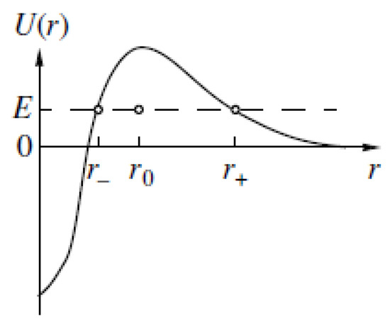
Figure 1. Typical dependence of effective Schrödinger potential U on r for a charged particle in an electric central-symmetric potential well, $r_{\pm }$ are turning points, and $r_0$ corresponds to maximum of the effective potential U. The dashed line describes the quasistationary level with $ϵ<-m$.

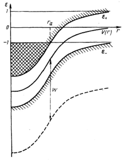
Figure 2. Illustration of the deformation of the upper and lower continua in a strong external electric field (the boundaries of the continua are shaded). Electrons that belong to the vacuum shell in the upper continuum fill the cross-hatched region. The states below the curve ${ϵ}_{-}/m=V(r)/m-1$ form the unobservable Dirac sea. The quantity W shows an artificial cutoff energy.

For $Z<Z_{\mathrm{cr}}$ electrons of the lower continuum (with $ϵ<-m$), fill all energy levels according to the Dirac picture of the electron-positron vacuum. They are spatially distributed at large distances. For $Z>Z_{\mathrm{cr}}$ the process of the tunneling of the electron of the lower continuum to the empty (localized) state that was prepared in the upper continuum with $ϵ<-m$ can be treated as the tunneling of the virtual positron (electron hole) with ${ϵ}_{e^{+}}=-{ϵ}_0-i\mathsf{\Gamma }/2$ from the region of the potential well to infinity, where it already can be observed. If one scatters an external real positron with a resonance energy ${ϵ}_{e^{+}}\simeq -{ϵ}_0>m$ on such a potential, this positron, for a short time, forms a resonance quasistationary state in the effective potential, which, after passage of a time $\sim 1/\mathsf{\Gamma }$, is decayed. As the result, the positron goes back to infinity. After that, during a time of the same order of magnitude, two positrons, being produced in a fluctuation together with two electrons, go off to infinity and those two electrons fill the stationary negative-energy state, as was explained.

If the ground state level was initially occupied by two electrons of opposite spins, then, at adiabatic change of the potential (in the sense clarified above), they remain on this level $ϵ={ϵ}_0$. At the adiabatic change of the potential, electrons have no energy to escape anywhere from this level. The production of pairs does not occur, since the level is occupied by electrons. During a time $\sim 1/\mathsf{\Gamma }$, their charge $2e<0$ is redistributed over the range of energies ${ϵ}_0-\mathsf{\Gamma }\left({ϵ}_0\right)/2\lesssim ϵ\lesssim {ϵ}_0+\mathsf{\Gamma }\left({ϵ}_0\right)/2$. This charge is localized at distances ($\sim 1/\left(3m\right)$ that are typical for the ground state in the Coulomb field [7]). In this sense, one formally requires a many-particle description of the stationary electron with $\mathrm{Re}{ϵ}_0<-m$ at $\mathsf{\Gamma }\ne 0$. However, neglecting a tiny $\mathsf{\Gamma }$ correction, for the finding of $ϵ\left(Z\right)$, one may continue to employ the one-particle description. If the experimenter scatters an external positron with ${ϵ}_{e^{+}}\simeq -{ϵ}_0>m$ on such a potential, the positron annihilates with one of the two electrons have occupied the ground-state level. After the passage of a time $\sim 1/\mathsf{\Gamma }$, there occurs spontaneous production of the one new pair, the electron fills empty state (after that, again, two electrons occupy the ground-state level) and the positron goes to infinity.

1.2. Semiclassical Approximation

Semiclassical approximation is one of the most important approximate methods of quantum mechanics [37]. Classical and semiclassical ideas are widely used in quantum field theory in problems dealing with the spontaneous vacuum symmetry breaking for bosons, cf. [21,36,38], in condensed matter physics, cf. [39,40,41], and in physics of nuclear matter [42,43].

As a consequence of the instability of the boson vacuum in a strong external field, there appears a reconstruction of the ground state and there arises a condensate of the classical boson field [44,45]. Many-particle repulsion of particles in the condensate provides the stability of the ground state. After that, excitations prove to be stable, cf. [42,43]. They are also successfully described using semiclassical methods, e.g., such as the loop expansion [36,46].

For fermions, there exist two possibilities. In the first situation, fermions heaving attractive interaction, being rather close to each other, may form Cooper pairs, cf. [40]. In the second situation, which we focus on here, electron-positron pairs, being produced in a strong static electric field, are well separated from each other by the potential barrier. Consequently, the electric potential attracts particles of one sign of the charge and repels antiparticles. Because of the Pauli principle, each unstable single-particle state is occupied by only one fermion. Therefore, it is natural to prolong a single-particle description in a overcritical region (until there appeared still not too many dangerous states). Classical approximation does not work for fermions, but semiclassical methods prove to be working. As is known, the semiclassical approach yields correct results for the values of the energy levels with big quantum numbers and in the case of spatially smooth potentials, when $d\tilde{\lambda }/dx\ll 1$, where $\tilde{\lambda }=1/p\left(x\right)$ is the reduced electron De Broglie length, $p\left(x\right)$ is the momentum, and x is the coordinate. For the Coulomb field for the ground-state level, a rough estimate yields $d\tilde{\lambda }/dr\sim 1/\left(Z{e}^2\right)$ for $r\to 0$. However, even for $d\tilde{\lambda }/dx\sim 1$, semiclassical approximation continues to work not bad in calculation of the energy levels, with an error not larger than 10% due to the presence of a numerically small parameter $\sim 1/{\pi }^2$, cf. [37].

Instability of the vacuum near a nucleus heaving a supercritical charge. It proves to be that the semiclassical approximation is applicable with an appropriate accuracy for the description of the electron energy levels in the supercritical field of a nucleus with the supercritical charge $Z>(170-173)$. Semiclassical approximation allows for finding rather simple expressions for the critical value of the charge, cf. Refs. [8,47,48], for energies of deep levels as a function of Z and for the probabilities of the penetration of the barrier between continua, cf. [3,4,5,6,7].

The spontaneous positron production in low-energy heavy-ion collisions. A comparison of the theory and experiment should check the application of QED in the region of strong fields outside the applicability of the perturbation theory. The description of the spontaneous production of positrons in heavy-ion collisions needs a solution of the two-center problem for the Dirac equation. Because variables are not separated in this case, the problem does not allow for the analytical treatment and numerical calculations are cumbersome. However, the use of the semiclassical approximation results in simple analytical expressions for the energies of the electron levels, cf. [6,7], valid with error less than few %. Thereby, this is one more example of the efficiency of the semiclassical approach.

Electron condensation in a field of a supercharged nucleus. In supercritical fields, many energy levels cross the boundary of the lower continuum and the problem of the finding of the vacuum charge density becomes of purely many-particle origin. It can be considered within the relativistic Thomas-Fermi method, cf. [2]. All of the initially empty states, which crossed the boundary $ϵ=-m$, are filled after a while. In this sense, one may speak about “electron condensate”.

Vacuum polarization and electron condensation at super-short distances from Coulomb center. In spite of the successes in explanation of all purely electrodynamical phenomena, QED is a principally unsatisfactory theory, since relations between the bare mass and charge and observable ones contain divergent integrals [49,50]. As the result, as one thinks, there is no not contradictive manner to pass from super-short to long distances. In spite of this, as is well known, it is possible to remove divergencies from all observable quantities with the help of the renormalization procedure.

The problem of the so-called “zero charge” or Moscow zero, cf. [51,52], is one of central problems related to renormalization of the charge. When considering the square of the charge of electron $e^2\left(r\right)$ as a function of the radius r and assuming finite value of the bare charge $e^2\left(r_0\right)=e_0^2>0$ for the source-size $r_0\to 0$, one derives $e^2(r\to \infty )\to 0$ instead of an expected value $e^2(r\to \infty )\to e^2=1/137$. The same problem appears, when one considers the screening of the central source with the charge density $n_{\mathrm{ext}}=Z_0\delta (r-r_0)$ for $r_0\to 0$, cf. [3]. The problem of a distribution of the charge near an external source of the charge with the radius $R\ll 1/m$, as well as the problem of the distribution of the charge of the electron at distances $r\ll 1/m$ are the key principal problems of QED. The semiclassical approach proves to be very promising in the calculation of the vacuum dielectric permittivity in strong inhomogeneous electric fields [53]. The density of the polarized charge is supplemented by the density from the electron condensation [3,42]. The problem proves to be specific and it depends on whether the radius of the external source of the charge is larger than a distance $r_{\mathrm{pole}}$, where the dielectric permittivity decreases to zero, or smaller $r_{\mathrm{pole}}$, cf. [54,55]. References [54,55] argued for the condensation of electron states in the upper continuum at distances larger than $r_{\mathrm{pole}}$ for $r_0>r_{\mathrm{pole}}$ and for the condensation of electron states originated in the lower continuum at distances smaller than $r_{\mathrm{pole}}$ (for $r_0<r_{\mathrm{pole}}$), at which the dielectric permittivity proves to be negative and $e_0^2<0$. The semiclassical consideration of this problem allows for presenting arguments in favor of a logical consistency of QED.

Similar effects in semimetals and in stack of graphene layers. The existence of the Weyl semimetals, i.e., materials with the points in Brillouin zone, where the completely filled valence and completely empty conduction bands meet with a linear dispersion law, $ϵ=v_{\mathrm{F}}p$, where the Fermi velocity is $v_{\mathrm{F}}\sim {10}^{-2}$, has been predicted in [56]. Systems with the relativistic dispersion law are likely to be realized in some doped silver chalcogenides, pyrochlore iridates, and in topological insulator multilayer structures. Weyl semimetals are three-dimensional analogs of graphene [57], where the energy of excitations is also approximately presented by the linear function of the momentum, but the electron subsystem is a two-dimensional one, whereas the photon subsystem remains three-dimensional. Even though the mass of excitations $m=0$ for ideal graphene and Weyl semimetals without interactions, a non-zero mass, $m\ne 0$, can be induced in many ways [58], resulting in a dispersion relation characterized by a gap, i.e. ${ϵ}^2=p^2{v}_{\mathrm{F}}^2+m^2{v}_{\mathrm{F}}^4.$ In difference with a small value of the fine structure constant in QED, $e^2=1/137$, the effective coupling in Weyl semimetals and in graphene is ${\alpha }_{\mathrm{ef}}=e^2/v_{\mathrm{F}}{\epsilon }_0$, where ${\epsilon }_0$ is the dielectric permittivity of the substance. The coupling constant ${\alpha }_{\mathrm{ef}}$ can be as $\ll 1$ as $\gtrsim 1$, depending on the substance, and both weak and strong coupling regimes are experimentally accessible. Thus, Weyl semimetals and an infinite stack of graphene layers make it possible to experimentally study various effects have been considered in 3+1 quantum electrodynamics (QED) for weak and effectively strong couplings, cf. [59,60].

Not concerning spontaneous production of positrons of our interest here, the electron-positron production in heavy-ion collisions was studied in many papers, cf. [61,62,63,64].

Additionally, electron-positron pair production from the vacuum can be triggered by the laser electromagnetic fields, e.g., see [65,66,67,68,69,70,71,72]. However it seems unlikely to realize such a possibility at least in the nearest future, cf. [73] and the references therein.

Electric fields with the strength $E\gg m^2$ may exist in astrophysical environments, e.g., they may occur at phase transitions in neutron and hybrid stars [43,74] and in neutron star mergers [75], and they also exist at surfaces of hypothetical nuclearites and abnormal superheavy nuclei [43,53,76,77,78].

Various radiative corrections to the deeply bound electron levels should certainly be taken into account, e.g., cf. [79,80,81] and the references therein. These higher-order corrections will not be considered in the given paper.

Below, attention is focused on a semiclassical description. I describe the instabilities of the boson and fermion vacua in static potentials, in particular in the Coulomb field. Afterwards, focus is concentrated on the description of the spontaneous positron production in low-energy heavy-ion collisions. Next, a many-particle semiclassical description of the electron condensation is considered. Finally, modification of the Coulomb field at super-short distances due to the vacuum polarization and electron condensation is studied.

The paper is organized, as follows. Section 2 starts with a brief discussion of instability for the charged bosons in static electric fields, in particular in the Coulomb field of a point-like nucleus with the charge $Z>Z_{\mathrm{cr}}=1/\left(2e^2\right)$. The behavior of deeply bound electrons obeying the Dirac equation in the strong static electric fields is considered in Section 3. First, I consider the case of a one-dimensional field and then of a spherically symmetric field. The Dirac equation is transformed to equivalent Schrödinger form in an effective potential and the interpretation of the solutions is discussed. Subsequently, in Section 3.5, I demonstrate exact solution of the problem of bound states in the strong Coulomb field of a point-like center. The focus is made on the problem of the falling of the electron to the center for a nucleus with the charge $Z\ge 1/e^2$. Section 3.6 describes how the problem is resolved while taking into account that nuclei have a finite size. In Section 4, I introduce a semiclassical approach to the Dirac equation, being transformed to the second-order differential equation. Electron levels crossed the boundary of the lower continuum are considered. The mean radius of the K-electron shell and the critical charge of the nucleus are found for $ϵ=-m$, as well as the number of levels that crossed the boundary of the lower continuum and their energies. The critical charge of the nucleus for the muon is also found. A comparison of semiclassical expressions with much more cumbersome exact expressions permits understanding the merits of the semiclassical approach. In Section 5, a semiclassical approximation is developed for the system of linear Dirac equations. Semiclassical wave functions in classically allowed and forbidden regions are introduced, and the Bohr–Sommerfeld quantization rule is formulated. Next, the probability of the positron production is calculated. Subsequently, semiclassical approximation is applied to non-central potentials. In Section 6, focus is concentrated on problems of the spontaneous positron production in low-energy collisions of heavy ions. The energies of deep levels as a function of the distance between colliding nuclei and the angular distribution of the positron production are found while employing semiclassical approach. Subsequently, I consider a screening of the charge at collisions of not fully striped nuclei. Semiclassical approximation (imaginary time method) is adequate for describing dynamics of the tunneling of electrons from the lower continuum to the upper one. In such a way, a correction on non-adiabaticity to the probability of the production of positrons is found. The electron condensation in the field of a supercharged nucleus is considered in Section 7. Section 8 presents the effects that are associated with the polarization of the electron-positron vacuum in weak and strong fields. Subsequently, in Section 9, I focus on the description of the charge distribution at super-short distances from the charge source. The effects of polarization of the vacuum and the electron condensation in the upper and lower continua will be considered. Section 10 contains a conclusion.

2. Relativistic Spinless Charged Particle in Static Field ${\mathit{A}}^{\mathit{\mu }}=({\mathit{A}}^{\mathbf{0}},\overrightarrow{\mathbf{0}})$

2.1. Reduction of Klein-Gordon-Fock Equation to Schrödinger Equation

Consider a spinless negatively charged boson placed in a stationary attractive potential well V. The Klein–Gordon–Fock equation renders

$$\Delta \varphi +[{(ϵ-V)}^2-m^2]\varphi =0.$$

(1)

With the help of notations

$$E=\frac{{ϵ}^2-m^2}{2m},U_{\mathrm{ef}}=-\frac{V^2-2ϵV}{2m},$$

(2)

we may rewrite Equation (1) in the form of the Schrödinger equation,

$$\Delta \varphi +2m(E-U_{\mathrm{ef}})\varphi =0.$$

(3)

As we see from Equation (2), for relativistic particles there appears to be an attractive term in the effective potential $-V^2/\left(2m{c}^2\right)$, even for a purely repulsive potential V. In the limit case $E\ll m$ and $|V|\ll m$, we have $ϵ\simeq m+E$ and $U_{\mathrm{ef}}\simeq V$, and we recover the Schrödinger equation for a nonrelativistic particle. For $|ϵ|<m$ the “nonrelativistic” energy is $E<0$, which corresponds to bound states in the interval of energies $-m<ϵ<m$. For a sufficiently deep potential well, the energy of the ground state level may cross the boundary $ϵ=-m$. In a deeper potential, other levels cross this boundary. For $ϵ<-m$, here $\mathrm{Re}E>0$, the levels become quasistationary, see Figure 1.

A comment is in order (D. N. Voskresensky 1974, see comment in [82]). For a spinless particle under consideration, the ground-state single-particle level only crosses the boundary $ϵ=-m$ for far-distant potentials, when $-V(r\to \infty )>C_{\mathrm{cr}}/r^2$, for a constant $C_{\mathrm{cr}}>0$. For potentials obeying condition $-V(r\to \infty )<C_{\mathrm{cr}}/r^2$, there appears to be a bound state for the antiparticle. In both cases for a broad potential well of a typical radius $R\gg 1/m$ the vacuum instability occurs at $|V|\simeq {|V|}_{\mathrm{cr}}\simeq 2m(1\pm O(1/\left(m^2{R}^2\right))$ either at ${ϵ}_{\mathrm{cr}}=-m$ or at ${ϵ}_{\mathrm{cr}}\simeq -m(1-O(1/\left(m^2{R}^2\right))$. In the case of a broad potential well, solutions of many-particle problems in both cases are almost the same, cf. [36]. For $-V>-V_{\mathrm{cr}}$ there appears production of pairs. Positively charged antiparticles go to infinity and negatively charged particles form a condensate, see [36,42].

Let us illustrate how the deformation of boundaries of upper and lower continua occurs in a static electric field forming a broad potential well for a negatively charged particle, cf. [2]. To be specific, consider a spherically symmetric field. Boundaries of continua, ${ϵ}_{\pm }$, are determined by

$${\overrightarrow{p}}^2\left(r\right)={({ϵ}_{\pm }-V)}^2-m^2=0.$$

(4)

They are shown in Figure 2. In upper and lower continua $p^2\left(r\right)>0$, these are classically allowed regions. In the gap between continua $p^2\left(r\right)<0$. This is a classically forbidden region. For $V<V_{\mathrm{cr}}=-2m-O(1/\left(m^2{R}^2\right))$, there arises a region of the overlapping of the continua that means that the negatively charged particle may penetrate from the lower continuum (from the exterior of the potential well) to the upper one (to the interior of the well).

With an exponential accuracy, the probability of a passage of the one-dimensional barrier is determined by

$$W\sim e^{-2\mathrm{Im}S}\sim e^{-2{\int }_{x_1}^{x_2}|p|dx},$$

(5)

where $x_1$ and $x_2$ are the turning points at which $p\left(x\right)=0$. This expression is applicable for $W\ll 1$.

As example, consider a uniform static electric field $eE=-\nabla V=const$, $|eE|\ll m^2$. Then we have $p\simeq \sqrt{{(ϵ+eEx)}^2-m^2}$. From Equation (5), we immediately obtain

$$W\sim e^{-\pi E_0/E},E_0=m^2.$$

(6)

This expression coincides with the first term of the infinite series solution [83].

A question arises as to whether it is possible to observe a process of the production of pairs already in a weak attractive electric field with the strength $|E|\ll m^2$ at $-\delta V>2m$? The critical difference $-\delta V\simeq -2m$ can be easily reached in the field of the capacitor, where $\nabla A_0=const$, at the increase of the distance d between plates. Employing $|\nabla A_0|=|\overrightarrow{E}|\sim {10}^4$ V/cm, the value, which is easily produced in electrical engineering, we estimate $|\delta V|>2m_{\pi }$ already for $d\gtrsim {10}^3$ cm. Here, $m_{\pi }\simeq 140$ MeV is the mass of the lightest charged boson, the pion. However the probability of the production of the pairs $W\sim e^{-2\mathrm{Im}S}$, $\mathrm{Im}S={\int }_{x_1}^{x_2}|p|dx$, is negligibly small at these conditions. Indeed, for $V=-eEx$, we get $\mathrm{Im}S={\int }_{x_1}^{x_2}|p|dx=\frac{\pi }{2}\frac{E_0}{E}.$ For pions $E_0\simeq {10}^{21}$ V/cm. For electrons $E_0\simeq 1.3·{10}^{16}\mathrm{V}/\mathrm{cm}$.

2.2. Relativistic Spinless Charged Particle in Coulomb Field of Point-Like Center

In the case of the Coulomb field of a point-like nucleus, $V=-Z{e}^2/r$, with the help of the replacement $\varphi (\overrightarrow{r})=R\left(r\right)Y_{lm}$, we obtain equation for the radial wave function $R\left(r\right)$ in the form

$${\Delta }_{r}R+2m\left[E+\frac{{\left(Z{e}^2\right)}^2}{2m{r}^2}-\frac{l(l+1)}{2m{r}^2}+\frac{ϵZ{e}^2}{mr}\right]R=0,{\Delta }_r=\frac{1}{r}\frac{{\partial }^2\left(rR\right)}{\partial r^2},$$

(7)

where $E=\frac{{ϵ}^2-m^2}{2m}$ is the effective nonrelativistic Schrödinger energy of the particle,

$$U_{\mathrm{ef}}\left(r\right)=-\frac{{\left(Z{e}^2\right)}^2}{2m{r}^2}+\frac{l(l+1)}{2m{r}^2}-\frac{ϵZ{e}^2}{mr}$$

(8)

is the effective potential, now, depending on l. Equation (7) and the ordinary Schrödinger equation for the radial function in the effective potential coincide after undertaking replacements

$$l(l+1)-{\left(Z{e}^2\right)}^2=\lambda (\lambda +1),ϵZ{e}^2/m\to Z^{\prime }{e}^2$$

(9)

in the former one. Thus, instead of the expression for the energy of the Schrödinger particle in the Coulomb field, we derive

$$E_{n_r,l}=-\frac{{\left(Z^{\prime }{e}^2\right)}^{2}m}{2{(n_r+\lambda +1)}^2}.$$

(10)

Here, $n_r+\lambda +1=n+\lambda -l$, $n_r=0, 1,\dots$ is the radial quantum number. Solving Equation (9) and retaining solution with positive-sign square root, $\lambda =-\frac{1}{2}+\sqrt{{(l+\frac{1}{2})}^2-{\left(Z{e}^2\right)}^2}$, because, for $Z=0$, $l=0$, one should have $\lambda =0$, we find the Sommerfeld formula for a spinless particle,

$${ϵ}_{n_r,l}^2=\frac{m^2}{1+\frac{Z^2{e}^4}{{(n-l-1/2+\sqrt{{(l+1/2)}^2-{\left(Z{e}^2\right)}^2})}^2}}.$$

(11)

There are two square-root solutions of this equation. Solution, which yields $ϵ\to m$ for $Z{e}^2\ll 1$, $n=1$, $l=0$, describes a negatively charged particle in the attractive Coulomb field ($Z>0)$. Solution, which yields $ϵ\to -m$ for $Z{e}^2\ll 1$, $n=1$, $l=0$, $Z>0$, after a change of $ϵ\to -ϵ$ describes the positively charged particle of the same mass in the field $Z<0$, since Equation (1) does not change under simultaneous replacement $ϵ\to -ϵ$ and $Z\to -Z$.

In the limit $Z{e}^2\ll 1$, Equation (11) for a negatively charged spinless boson, in the ground state ($n=1$, $l=0$), produces $ϵ\to m-\frac{{\left(Z{e}^2\right)}^{2}m}{2n^2}$ in accordance with the result for the Schrödinger particle.

For $Z>Z_{cr}=1/\left(2e^2\right)$ the particle, being in the ground state ($n=1$), falls down to the center. Let $Z{e}^2=1/2+\delta$ for $0<\delta \ll 1$. Subsequenty, choosing positive-sign square root of solution (11) we have for $Z{e}^2=1/2+\delta$, $ϵ\simeq \frac{m(1+i\delta )}{\sqrt{2}}$ and the wave function

$$\varphi \propto e^{-iϵt}\propto e^{m\delta t/\sqrt{2}}\to \infty \mathrm{for}t\to \infty ,$$

is not normalized, reflecting the fact of the falling of the negatively charged particle to the Coulomb center with $Z>0$ and the falling of the positively charged particle to the Coulomb center at $Z<0$. We dropped the negative-root solution of Equation (11) as not physical one, since it arises at $ϵ\simeq -m$ already for small $Z>0$. However, note that the negative-root solution of Equation (11), $-\frac{m(1+i\delta )}{\sqrt{2}}$, for the negatively charged particle near the Coulomb center for $Z>Z_{\mathrm{cr}}=1/\left(2e^2\right)$ yields $\varphi \propto e^{-m\delta t/\sqrt{2}}$, i.e., decreasing at $t\to \infty$. This implies a possibility of a multi-particle interpretation of the $ϵ<0$ solution for the negatively charged particle in the field $Z>0$. We return to this question in Section 9.2.

The value $Z_{cr}=68.5$. It means that the Mendeleev table would be closed on element with $Z_{cr}=68$, if the nuclei were point-like. As we have mentioned, the lightest spinless meson is the pion. The radius of the real nucleus with atomic number A is found from the condition $4\pi {\rho }_0{R}^3/3=A$, where ${\rho }_0\simeq 0.16$ fm${}^{-3}\simeq 0.48m_{\pi }^3$. For a symmetric nucleus $A\simeq 2Z$ we estimate $R>a_{1\mathrm{B}}^{\pi }=1/\left(m_{\pi }Z{e}^2\right)$ (radius of the ground-state orbit for the pion) already for $Z>40$. Subsequently, the lowest pion orbit enters inside the nucleus and approximation of a point-like nucleus becomes invalid.

Note that, for $Z=Z_{\mathrm{cr}}$, ${ϵ}_{\mathrm{part}}+{ϵ}_{\mathrm{a}.\mathrm{part}}=m\sqrt{2}>0$, and thereby pairs are not produced at such conditions. This peculiarity appears only for the case of the point-like Coulomb field. For a field, being cut at $R\ne 0$ ($R\ll 1/m_{\pi }$, such that $V=-Z{e}^2/r$ for $r>R$ and $V=-Z{e}^2/R$, the model I, or for $V=-\frac{Z{e}^2}{R}(\frac{3}{2}-\frac{r^2}{R^2})$, the model II at $r<R$, the ground state particle level continues to decrease with increasing Z and decreasing R and for $Z=Z_{\mathrm{cr}}\left(R\right)>Z_{\mathrm{cr}}$, it reaches $ϵ=-m$. At $Z=Z_{\mathrm{cr}}\left(R\right)$, the sum ${ϵ}_{\mathrm{part}}+{ϵ}_{\mathrm{a}.\mathrm{part}}$ is zero, corresponding to the spontaneous production of the pairs for $Z\ge Z_{\mathrm{cr}}\left(R\right)$, at $R<R_{\mathrm{cr}}$.

Sommerfeld formula for electron. Electron has spin $1/2$. In the absence of the magnetic field spin and orbital spaces are orthogonal. Thus one may expect that expression (11) continues to hold also for electron after replacement $l+1/2\to |\overrightarrow{J}|+1/2=|\kappa |$, where $\kappa =-1, 0, 1\dots$ is integer number, since axial vectors of angular momentum and spin are summed up, $\overrightarrow{L}\to \overrightarrow{J}=\overrightarrow{L}+\overrightarrow{s}$. Subsequently, we have

$${ϵ}_{n_r,\kappa }^2=\frac{m^2}{1+\frac{Z^2{e}^4}{{(n_r+\sqrt{{\kappa }^2-{\left(Z{e}^2\right)}^2})}^2}},$$

(12)

where $n_r=n-|\kappa |=0, 1,\dots$ is a radial quantum number. Now, falling to the center appears when the ground state level reaches the value $ϵ=0$. It occurs for $Z=Z_{\mathrm{cr}}=1/e^2=137$. For a field cutted at $R\ne 0$, e.g., for the case $V=-Z{e}^2/r$ for $r>R$ and $V=-Z{e}^2/R$ for $r<R$, the ground state level continues to decrease with increasing Z and for $Z=Z_{\mathrm{cr}}\left(R\right)>Z_{\mathrm{cr}}$ it reaches $ϵ=-m$. After that, the sum ${ϵ}_{\mathrm{part}}+{ϵ}_{\mathrm{a}.\mathrm{part}}$ reaches zero, corresponding to the spontaneous production of the electron-positron pairs. Two electrons occupy the ground-state level and two positrons with $-ϵ>m$ move to infinity.

Note that the same expression (12) is derived from the exact solution of the Dirac equation in the Coulomb field, as we will see in Section 3.5.

3. Dirac Equation for Particle in Static Electric Field, ${\mathit{A}}^{\mathbf{\mu }}=({\mathit{A}}^{\mathbf{0}},\overrightarrow{\mathbf{0}})$

We are now at the position to focus on the problem of our main interest in this paper, i.e., to describe the behavior of electrons in a strong static electric field.

Interaction with 4-vector field $A^{\mu }=(A^0,\overrightarrow{A})$ is constructed with the help of minimal coupling

$$({\gamma }^{\mu }{\widehat{p}}_{\mu }-e{\gamma }^{\mu }{A}_{\mu }-m)\mathsf{\Psi }=0,$$

(13)

$p_{\mu }=i{\partial }_{\mu }$, ${\gamma }^{\mu }$ are ordinary Dirac matrices.

3.1. Dirac System in Case of One-Dimensional Electric Field

In the case of a static one-dimensional electric field ($\overrightarrow{A}=0$) using replacement

$$\mathsf{\Psi }=e^{-iϵt}\tilde{\psi }\left(x\right)$$

(14)

we rewrite Equation (13) as

$$(ϵ-V+i{\gamma }^0\overrightarrow{\gamma }\frac{d}{dx}-{\gamma }^{0}m+V\left(x\right))\tilde{\psi }\left(x\right)=0.$$

(15)

We may rewrite Equation (15) as

$${\tilde{\psi }}^{\prime }={\hslash }^{-1}\widehat{D}\tilde{\psi },\widehat{D}=\left(\begin{array}{ccc}0& & m+ϵ-V\\ m-ϵ+V& & 0\end{array}\right),\tilde{\psi }=\left(\begin{array}{c}G\\ F\end{array}\right).$$

(16)

For further convenience, here we retained dependence on ℏ.

3.2. Dirac System in Central-Symmetric Field

Introducing

$$\begin{array}{c}\hfill {\psi }_{jlm}=\frac{1}{r}\left(\begin{array}{c}G\left(r\right){\mathsf{\Omega }}_{jlM}\left(\overrightarrow{n}\right)\\ iF\left(r\right){\mathsf{\Omega }}_{j{l}^{\prime }M}\left({\overrightarrow{n}}^{\prime }\right)\end{array}\right),{\mathsf{\Omega }}_{j{l}^{\prime }M}=-\overrightarrow{\sigma }\overrightarrow{n}{\mathsf{\Omega }}_{jlM}(\overrightarrow{n}),\end{array}$$

(17)

where ${\mathsf{\Omega }}_{jlM}$ is the spherical spinor, $j,M$ are full angular momentum and its projection, $j=l\pm 1/2$, l is the orbital angular momentum, $l+l^{\prime }=2j$, $\overrightarrow{n}=\overrightarrow{r}/r$, $|\kappa |=j+1/2$.

After the separation of angular and spin variables, the Dirac system becomes

$${\psi }^{\prime }={\hslash }^{-1}\widehat{D}\psi ,\widehat{D}=\left(\begin{array}{ccc}-\tilde{\kappa }/r& & m+ϵ-V\\ m-ϵ+V& & \tilde{\kappa }/r\end{array}\right),\psi =\left(\begin{array}{c}G\\ F\end{array}\right),$$

(18)

$\tilde{\kappa }=\hslash \kappa$, $|\kappa |=j+1/2$. The ground state corresponds to $\kappa =-1$. The one-dimensional result, see (16), follows from (18) provided one puts $\kappa =0$ and replaces $d/dr\to d/dx$.

3.3. Reduction of Dirac System to Schrödinger Equation

With the help of the replacement

$$\varphi ={(m+ϵ-V)}^{-1/2}G,$$

(19)

Equation (18) is reduced to the equation of the second-order in r-derivative, similar to the Schrödinger equation,

$${\varphi }^{″}+p^2\left(r\right)\varphi =0,p^2=2m(E-U_{\mathrm{ef}}\left(r\right)),$$

(20)

where

$$E=\frac{{ϵ}^2-m^2}{2m},U_{\mathrm{ef}}\left(r\right)=\frac{ϵV}{m}-\frac{V^2}{2m}+\frac{\kappa (1+\kappa )}{2r^{2}m}+U_s,$$

(21)

$$U_s=\frac{1}{4m}\left[\frac{V^{″}}{m+ϵ-V}+\frac{3}{2}{\left(\frac{V^{\prime }}{m+ϵ-V}\right)}^2-\frac{2\kappa V^{\prime }}{r(m+ϵ-V)}\right]$$

(22)

is the term appeared due to the spin. If $U_s$ were zero, after the replacement $\kappa \to l$ we would recover the Klein–Gordon–Fock equation for a spinless particle.

At $r\to 0$, for $V=-Z{e}^2/r$, we have $U_s\to -\frac{1+4\kappa }{8m{r}^2}$. For 1 s level $\kappa =-1$, $U_s\to \frac{3}{8m{r}^2}$. In the latter case

$$U_{\mathrm{ef}}\left(r\right)\to -\frac{{\left(Z{e}^2\right)}^2}{2m{r}^2}+\frac{3}{8m{r}^2}$$

(23)

for $r\to 0$. The falling to the center in such a Schrödinger potential occurs when $U_{\mathrm{ef}}\left(r\right)<-1/\left(8m{r}^2\right)$, cf. [84], which corresponds to $Z{e}^2>1$.

3.4. Interpretation of Bound States in a Weak Field

The Dirac equation describes the electron and positron simultaneously. Therefore at appearance of the bound state in a potential well there arises a question regarding whether it relates to the electron or to the positron. As example, consider the case of a weak external static central-symmetric electric field produced by a static source of a positive charge distributed in a range r. Subsequently, $V=-\zeta v\left(r\right)<0$ for the electron, where $\zeta >0$ is a parameter proportional to the depth of the potential well. As is known, for sufficiently small $\zeta$, the Dirac equation, as the Klein–Gordon–Fock equation, can be transformed to the Schrödinger equation for a nonrelativistic particle. The bound state for the electron appears first at a certain value of $\zeta$. At decreasing $\zeta$, this state is diluted in the continues spectrum with $ϵ\ge m$.

The system of Dirac Equation (18) is symmetric in respect to replacements $ϵ\to -ϵ$, $V\to -V$, $\kappa \to -\kappa$, $G\to F$. Equation describing energy levels does not depend on G and F. Thereby, it is symmetric, respectively, replacements $ϵ\to -ϵ$, $V\to -V$, $\kappa \to -\kappa$. In the case of the source of a positive charge, the electron undergoes attraction. In the field of the opposite-sign charge ($V\to -V$), the electron undergoes repulsion. Because, in the attractive field, there appears the electron energy level going from the upper continuum, in the repulsive field there appears the electron energy level originating from the lower continuum. However, because the Dirac equation simultaneously describes electron and positron, if the electron moves in a repulsive field, then the positron moves in an attractive one. Thereby, the electron level moving in a repulsive field from the lower continuum can be interpreted as the positron level ($ϵ\to -ϵ$, $\kappa \to -\kappa$) going from the upper continuum (now in the field of attraction to the positron). It is natural to think that in a weak repulsive field for the electron for a small $\zeta <0$ a deeply bound level with $ϵ\simeq -m$ should not exist. Because such a state nevertheless exists in the full set of solutions of the Dirac equation, after the replacement $ϵ\to -ϵ$, $\kappa \to -\kappa$, it should be interpreted as the positron state. This interpretation is confirmed experimentally. In the field of a proton, there are electron bound states lying near the boundary of the upper continuum but there are no positron states with $ϵ\simeq -m$. Vise versa, in the field of an antiproton, there exist positron levels with $ϵ\simeq m$, but there are no electron levels with $ϵ\simeq -m$. This picture is also established by the minimization of the energy in the mentioned cases. Namely, in the field of a positive charge, the presence of the bound electron is more energetically favorable when compared to the presence of the positron.

Statements done above seem obvious except the case, which I shall consider below in Section 9.2, when polarization of the vacuum may result in a negative dielectric permittivity and attraction is replaced by repulsion.

3.5. Exact Solution for Electron in Coulomb Field of Point-Like Center

Consider the discrete spectrum $ϵ<m$ of the Dirac equation in the potential $V=-Z{e}^2/r$. We search G and F in Equation (18) as

$$G=\sqrt{m+ϵ}{e}^{-\tilde{r}/2}{\tilde{r}}^g(Q_1+Q_2),F=-\sqrt{m-ϵ}{e}^{-\tilde{r}/2}{\tilde{r}}^g(Q_1-Q_2),$$

(24)

where

$$\tilde{r}=2r\sqrt{m^2-{ϵ}^2},g=\sqrt{{\kappa }^2-{\left(Z{e}^2\right)}^2}.$$

(25)

This form of the solution, cf. [49], follows from asymptotic behavior of $G,F\sim r^{\pm g}$ at $r\to 0$ and $G,F\sim e^{-\tilde{r}/2}$ at $r\to \infty$. Solutions $G,F\sim C_{1,2}{r}^{-g}$ are dropped (i.e., we put $C_{1,2}=0)$ due to the divergence of their contribution to the probability (${\int |\psi |}^{2}dr\to \infty$).

Setting (24) in Equation (18), we obtain a system of equations

$$\begin{array}{cc}& \tilde{r}{Q}_1^{\prime }+\left(g-\frac{Z{e}^2ϵ}{\sqrt{m^2-{ϵ}^2}}\right)Q_1+\left(\kappa -\frac{Z{e}^{2}m}{\sqrt{m^2-{ϵ}^2}}\right)Q_2=0,\\ & \tilde{r}{Q}_2^{\prime }+\left(g+\frac{Z{e}^2ϵ}{\sqrt{m^2-{ϵ}^2}}-\tilde{r}\right)Q_2+\left(\kappa +\frac{Z{e}^{2}m}{\sqrt{m^2-{ϵ}^2}}\right)Q_1=0.\end{array}$$

(26)

These equations are reduced to

$$\begin{array}{cc}& \tilde{r}{Q}_1^{″}+\left(2g+1-\tilde{r}\right)Q_1^{\prime }-\left(g-\frac{Z{e}^2ϵ}{\sqrt{m^2-{ϵ}^2}}\right)Q_1=0,\\ & \tilde{r}{Q}_2^{″}+\left(2g+1-\tilde{r}\right)Q_2^{\prime }-\left(g+1-\frac{Z{e}^2ϵ}{\sqrt{m^2-{ϵ}^2}}\right)Q_2=0.\end{array}$$

(27)

As is seen, Equation (27) are symmetric under simultaneous replacement $ϵ\to -ϵ$ and $Z{e}^2\to -Z{e}^2$.

The finite solution for $\tilde{r}\to 0$ gets the form

$$Q_1=AF\left(g-\frac{Z{e}^2ϵ}{\sqrt{m^2-{ϵ}^2}},2g+1,\tilde{r}\right),Q_2=BF\left(g+1-\frac{Z{e}^2ϵ}{\sqrt{m^2-{ϵ}^2}},2g+1,\tilde{r}\right),$$

(28)

where $F(\alpha ,\beta ,z)$ is the degenerate hypergeometric function. Setting $\tilde{r}=0$ in one of Equation (26), we find relation

$$B=-\frac{g-\frac{Z{e}^2ϵ}{\sqrt{m^2-{ϵ}^2}}}{\kappa -\frac{Z{e}^{2}m}{\sqrt{m^2-{ϵ}^2}}}A.$$

(29)

Both of the hypergeometrical functions in (28) are reduced to polynomials, otherwise they would grow as $e^{\tilde{r}}$ for $\tilde{r}\to \infty$, which results in the divergence of the probability. From this requirement follows that $\alpha$ in $F(\alpha ,\beta ,z)$ equals a non-positive integer number, i.e.,

$$g-\frac{Z{e}^2ϵ}{\sqrt{m^2-{ϵ}^2}}=-n_r,n_r=1, 2,\dots$$

(30)

For $n_r=0$, only one of two functions is reduced to a polynomial. Subsequenty, $g=\frac{Z{e}^2ϵ}{\sqrt{m^2-{ϵ}^2}}$ and $\frac{Z{e}^{2}m}{\sqrt{m^2-{ϵ}^2}}=|\kappa |$. If $\kappa <0$, then $B=0$ in Equation (29) and $Q_2=0$, and the required condition is fulfilled. If $\kappa >0$, then $B=-A$ and $Q_2$ is a divergent function at $n_r=0$. Thereby, permitted states are $n_r=0, 1,\dots$ for $\kappa <0$ and $n_r=1, 2,\dots$ for $\kappa >0$. From (30), it also follows the solution for the negatively charged particle with $ϵ<0$ for $Z<0$. In a single particle problem under consideration, one should drop such a solution, since it describes a strongly bound particle already in a weak field. However, such a solution can be appropriately treated within a many-particle picture with taking the vacuum polarization and the electron condensation that originated in the lower continuum into account, as we argue below in Section 9.2.

From (30), we obtain the Sommerfeld expression

$$ϵ=\pm m{\left[1+\frac{{\left(Z{e}^2\right)}^2}{{(\sqrt{{\kappa }^2-{\left(Z{e}^2\right)}^2}+n_r)}^2}\right]}^{-1/2},$$

(31)

cf. Equation (12). Note that, for $Z>0$, $Z<1/e^2$, only solution $ϵ>0$ follows from (30), since $n_r+g>0$. Thereby, “+” sign solutions (31) correspond to particles (electrons) in the field of the positively charged Coulomb center (or to antiparticles (positrons) in the field of the negatively charged Coulomb center). The “−” sign solutions (31), after replacements $ϵ\to -ϵ$, $\kappa \to -\kappa$ (after that “−” sign branch coincides with “+” sign branch) describe antiparticles with $ϵ>0$ in the field of negatively charged Coulomb center ($Z<0$).

The ground state 1 s-level of the electron in the field of the positively charged Coulomb center ($Z>0$) corresponds to $\kappa =-1$, $n_r=0$. Its energy is

$${ϵ}_0=m{g}_0,g_0=\sqrt{1-{\left(Z{e}^2\right)}^2}.$$

(32)

At $Z{e}^2\ge 1$, there occurs falling of the electron to the center. Indeed, for $r\to 0$ following (24), (27) we get

$$G=a_1{r}^g+a_2{r}^{-g},F=b_1{r}^g+b_2{r}^{-g}.$$

(33)

For $Z{e}^2=1+\delta >1$, the value $g=i\sqrt{2\delta }$ becomes imaginary and solutions oscillate as

$$C_{1}cos(|g|lnr)+C_{2}sin(|g|lnr),$$

(34)

that corresponds to not normalized probability ${\int }_0^{\infty }{|\psi |}^{2}dr$. At $Z{e}^2=1+\delta$, $0<\delta \ll 1$, solution of Equation (32) yields $ϵ=+im\sqrt{2\delta }$ and the electron wave function grows as $\mathsf{\Psi }\propto e^{+m\sqrt{2\delta }t}$, indicating the falling of the electron to the center. The solution of opposite sign (see Equation (31)) arises from the lower continuum at $V\to 0$. In the single-particle problem a negative-energy solution should be dropped. Note that at $Z{e}^2=1+\delta$, it yields $ϵ=-im\sqrt{2\delta }$ and $\mathsf{\Psi }\to 0$ at $t\to \infty$ that may suggest an interpretation. However, an appropriate interpretation proves to be possible only beyond the single-particle problem, as will be shown in Section 9.2.

Solutions (31) and (32) hold formally for the positron in the Coulomb potential of the nucleus with the charge $Z<0$. Within the single-particle problem under consideration, appropriate interpretation again exists for the solution, where energy originates from the upper continuum decreasing with increasing $-Z$, rather than the negative-energy solution, similarly to that happened for the electron at $Z>0$.

For $Z>0$, only two electrons (due to Pauli principle), if they have occupied the ground state, undergo falling to the Coulomb center for $Z{e}^2=1$. For levels with the quantum number $n_r>0$, we have ${ϵ}_{n_r,\kappa }>0$ for $Z=1/e^2$. Now, assume that the ground-state level was empty and we adiabatically increase Z. There is no appropriate solution of the single-particle problem for the point-like nucleus with $Z>1/e^2$ in this case.

Avoiding problem of falling to the center. A reasonable interpretation may appear, only if one assumes that the nucleus has a size $R\ne 0$, and then we may safely decrease R. First assume that $R\ll r_{\mathsf{\Lambda }}=1/m$. In the limit $\mathsf{\Lambda }=ln(r_{\mathsf{\Lambda }}/R)\gg 1$ for the ground-state level of the electron, one gets [15,16]

$${ϵ}_0(\zeta <1)=m{g}_0/\mathrm{th}\left(\mathsf{\Lambda }{g}_0\right),\mathrm{for}\zeta =Z{e}^2<1.$$

(35)

For $\zeta <1$, $\mathsf{\Lambda }{g}_0\gg 1$, the value $\mathrm{th}\left(\mathsf{\Lambda }{g}_0\right)\simeq 1-2e^{-2\mathsf{\Lambda }{g}_0}$ rapidly tends to unity and Equation (35) coincides with (32). For $R\ne 0$, the point $\zeta =1$ is already not a singular point for the function ${ϵ}_0\left(\zeta \right)$. Equation (35) is analytically continued in the region $\zeta >1$. For $\zeta$ close to unity, we have

$${ϵ}_0(\zeta >1)=m{\tilde{g}}_0/\mathrm{tg}\left(\mathsf{\Lambda }{\tilde{g}}_0\right),\mathrm{for}\zeta =Z{e}^2>1,$$

(36)

where ${\tilde{g}}_0=\sqrt{{\zeta }^2-1}$. At any $R\ne 0$ the curve ${ϵ}_0(\zeta >1)$ continues to decrease with increasing $\zeta$ and reaches the boundary of the lower continuum. It occurs at ${\zeta }_{\mathrm{cr}}=1+{\pi }^2/\left(2{\mathsf{\Lambda }}^2\right)+O\left({\mathsf{\Lambda }}^{-3}\right)$.

A comment is in order. The single-particle solution for $R\to 0$ should be modified. Indeed, for R as small as $R\sim r_{\mathrm{L}}\simeq r_{\mathsf{\Lambda }}{e}^{-3\pi /\left(2e^2\right)}$, the multi-particle effects of the polarization of the vacuum should be included, and the problem goes beyond the single-particle one, see the below consideration in Section 8.

3.6. Avoiding Problem of Falling to Center in Realistic Treatment. Spherical Nucleus of Finite Size

For the Coulomb field with the charge $Z<1/e^2$, the electron in the ground state is typically situated at distances $\sim a_{1\mathrm{B}}=1/\left(Z_{\mathrm{obs}}{e}^{2}m\right)>1/m$ and distribution of the charge $Z\left(r\right)$ at distances $r\sim R_{\mathrm{nucl}}\ll a_{1\mathrm{B}}$ almost does not affect the electron motion. In the realistic problem, the nucleus has a finite size, $R_{\mathrm{nucl}}\simeq r_N{A}^{1/3}\ll a_{1\mathrm{B}}$, where A is the atomic number, $r_N\simeq 1.2$ fm, and, thereby, the potential is smoothen at $r<R_{\mathrm{nucl}}$. The falling to the centrum does not occur, as it has been mentioned. Even for $Z\gg 1/e^2$, the electron density remains to be distributed at finite distances.

Taking into account of the distribution of the charge inside the nucleus, we have

$$V\left(r\right)=-\zeta f(r/R_{\mathrm{nucl}})/R_{\mathrm{nucl}}\mathrm{for}0<r<R_{\mathrm{nucl}},V=-\zeta /r,\mathrm{for}r>R_{\mathrm{nucl}}.$$

(37)

Two models have been employed in the literature: model I, when $f(x<1)=1$, that corresponds to the surface distribution of the charge, and model II, when $f(x<1)=(3-x^2)/2$, which describes distribution of protons with the constant volume density.

The energy shift of the electron level can be found with the help of the perturbation theory that is applied to the Dirac system (18). Following [16],

$$\beta =\frac{\partial ϵ}{\partial \zeta }=\int V\left(r\right)(G^2+F^2)dr/\zeta <0,$$

(38)

i.e., the curve $ϵ\left(\zeta \right)$ decreases monotonically with increasing $\zeta$ and crosses the boundary of the lower continuum with a finite value $\beta$. After that, $ϵ\left(\zeta \right)$ acquires an exponentially small imaginary part.

Because the exact solution of the Coulomb problem for $r>R$ looks rather cumbersome and for $r<R$ is impossible for a realistic cut of the potential, it is natural to use approximate methods. Most economical is a semiclassical approach. Here, we should notice that the replacement (19) becomes singular for $ϵ<-m$ in the point $V\left(r_1\right)=m+ϵ<0$. Because to this, the effective potential

$$U_{\mathrm{ef}}(r,ϵ)=\frac{3}{8m}{(r-r_1)}^{-2}+\dots \to \infty ,\mathrm{for}r\to r_1,$$

(39)

and semiclassical expressions loose their sense due to the divergency of the integral ${\int }^{r}2m{(E-U_{\mathrm{ef}}(r,ϵ))}^{1/2}dr$. However, this is only a formal problem, since the initial Dirac system (18) has no singularity at $r\to r_1$. To avoid the problem one should bypass the singular point in the complex plane, as one usually does bypassing turning points, or one may apply the semiclassical consideration straight to the linear Dirac equations. Note that, in the one-dimensional case corresponding to $\kappa =0$, see Equation (16), the mentioned singularity occurs in the turning points, and one may use standard semiclassical methods.

The probability of the spontaneous production of positrons is determined by the width of the corresponding electron level, $\mathrm{Im}ϵ$, for $\mathrm{Re}ϵ<-m$. Thus the width is found from the solution of the Dirac equation. The value $\mathsf{\Gamma }$, which determines probability of the positron production, $W\sim e^{\mathsf{\Gamma }t}$, can be expressed directly through components of the Dirac bispinor (G and F). It yields the flux of particles going to infinity (at normalization on one particle):

$$\mathsf{\Gamma }=\int {\psi }^{†}{\gamma }^0\overrightarrow{\gamma }\psi d\overrightarrow{f}=2\mathrm{Im}\left(F{G}^{*}\right){|}_{r\to \infty }.$$

(40)

4. Semiclassical Approach to Dirac Equation Transformed to Second-Order Differential Equation

4.1. Accuracy of Calculation of Energy Levels in Semiclassical Approximation

Substituting $\psi =A{e}^{iS/\hslash }$, where A and S are real quantities, in equation

$${\hslash }^2\Delta \psi +p^2\left(r\right)\psi =0$$

(41)

we find two equations

$${\hslash }^2\Delta A+p^{2}A=A{(\nabla S)}^2,i\hslash (2\nabla A\nabla S+A\Delta S)=0.$$

(42)

For a convenience, the dependence on ℏ is recovered here. The Hamilton–Jacobi equation for the action ${(\nabla S)}^2=p^2$ is obtained provided

$${\hslash }^2\frac{A^{″}}{p^{2}A}\sim \frac{{\hslash }^2}{{\left(pl\right)}^2}\sim {\left(\frac{d\tilde{\lambda }}{dr}\right)}^2\ll 1,\tilde{\lambda }=\frac{\hslash }{p},$$

(43)

where l is the typical size of the potential V. For the Coulomb potential at typical distances $r\sim 1/\left(2m\right)$ characterizing ground-state electron with $ϵ\simeq -m$ we have $p\sim \tilde{g}/r$. From estimate (43), we see that the semiclassical approximation for the wave function for such distances is accurate up to terms $1/{\tilde{g}}^2$, $\tilde{g}=\sqrt{{\zeta }^2-{\kappa }^2}$ for $\zeta >|\kappa |$.

Using the Bohr–Sommerfeld quantization rule, we have

$$\frac{{\hslash }^2}{{\left(pl\right)}^2}\sim \frac{{\hslash }^2}{{\left({\int }_{r_0}^{r_{-}}pdr\right)}^2}\sim \frac{1}{{\pi }^2{(n_r+\gamma )}^2},$$

(44)

where the phase $\gamma \sim 1$, $n_r=0,1,\dots$, $r_0$, and $r_{-}$ are the turning points separating the classically allowed region. Thus even in calculation of the energy of the levels with small quantum numbers one may consider on the error not larger that 10%.

Finally, let us notice that the transition from the Dirac equation in the external field to the corresponding more simple Hamilton–Jacobi equation has been used in many investigations, cf. [85,86,87]. The case of the deep electron levels, with the energy $ϵ\lesssim -m$, was studied in [3,4,5,6,7].

4.2. Semiclassical Approximation to Coulomb Field of Point-Like Nucleus

In the field $V=-\zeta /r$, for $\zeta <|\kappa |$, the semiclassical method results in exact expression for the energy spectrum. Let us show this. For that, we do replacements

$$G=\sqrt{\frac{m+ϵ}{r}}({\chi }_1+{\chi }_2),F=\sqrt{\frac{m-ϵ}{r}}({\chi }_1-{\chi }_2).$$

(45)

Subsequently, the system of two Dirac Equation (18) reduces to equations

$${\chi }_i^{″}+p_i^2\left(r\right){\chi }_i=0,i=1,2,$$

(46)

with

$$p_i\left(r\right)={\left[{ϵ}^2-m^2-\frac{2ϵ\zeta \pm \sqrt{m^2-{ϵ}^2}}{r}+\frac{{\zeta }^2-{\kappa }^2+1/4}{r^2}\right]}^{1/2}.$$

(47)

Adding the Langer correction to the effective potential results in replacements $p_i\to p_i^{*}$, we find

$$p_i^{*}\left(r\right)=\sqrt{-a+2b/r-g^2/r^2},a=m^2-{ϵ}^2,b=ϵ\zeta \pm \frac{1}{2}\sqrt{m^2-{ϵ}^2},g^2={\kappa }^2-{\zeta }^2.$$

(48)

Subsequently, applying the Bohr–Sommerfeld quantization rule, we have

$${\int }_{r_0}^{r_{-}}{p}_i^{*}dr=(a^{-1/2}b-g)\pi =(n_r+1/2)\pi .$$

(49)

From here, we recover the exact result (31). To get (31) from an exact solution of the Dirac equations, we have performed a cumbersome analysis of hypergeometric functions, whereas the semiclassical approach needs taking only one simple integral.

After replacements $b\to ϵ\zeta$, $g^2\to {(l+1/2)}^2-{\zeta }^2$, Equation (48) is also valid for spinless bosons. Performing integration leads us to the exact expression (11).

4.3. Finite Nucleus. Semiclassical Wave Functions and Quantization Rule

Certainly, it is also possible to apply semiclassical approach to Equation (20) with effective potential in the form (21), (22). In the range, where the parameter of applicability of semiclassical approximation is $|d\tilde{\lambda }/dr|\sim 1$, the usage of Dirac equations presented in different forms leads to slightly different results. For instance, applying (20) to the Coulomb field does not yield the exact result for the energy of the levels, although the accuracy of the approximation proves to be appropriate. For the electron energy $ϵ<-m$ the variable replacement (19) leads to the singularity in the point $r_1$, where $V\left(r_1\right)=m+ϵ<0$. Near this point, semiclassical expressions become invalid due to divergence of the contribution to the action $\int {\left[2m(E-U_{\mathrm{ef}})\right]}^{1/2}dr$. However, as it was mentioned, this circumstance is not reflected on the calculation of the energy levels, since $r_1$ is situated under the barrier, where wave functions prove to be exponentially small.

The electron energy levels can be found with the help of the Bohr–Sommerfeld quantization rule [3] applied to the Dirac equation presented in the form (20) with effective potential in the form (21), (22). We have

$${\int }_{r_0}^{r_{-}}{p}^{*}dr=(n_r+{\gamma }^{\prime })\pi .$$

(50)

Value $p^{*}$ is obtained from expression (20) after taking the Langer correction into account, i.e., after doing the replacement $\kappa (1+\kappa )/r^2\to {(\kappa +1/2)}^2/r^2$ in the expression for the effective potential. The value of the phase ${\gamma }^{\prime }$ depends on whether the turning point is inside the nucleus or outside it. In the latter case, the potential is $V=-\zeta /r$ and ${\gamma }^{\prime }=3/4$ for $\kappa =-1$ and ${\gamma }^{\prime }=1/2$ for $\kappa \ne -1$.

The contribution to the normalization of the semiclassical wave function from the classically forbidden region is usually dropped. In order to understand accuracy of this approximation consider the probability of the presence of the electron in sub-barrier region $r_{-}<r<r_{+}$:

$$W_0={\int }_{r_{-}}^{r_{+}}(G^2+F^2)dr.$$

(51)

To be specific, let us put $ϵ=-m$ and consider $\zeta \gg |\kappa |$. The wave function in the classically allowed region is [37]:

$$\chi =(c_0/\sqrt{p^{*}})sin({\int }_{r_0}^r{p}^{*}dr+\pi /4)dr.$$

(52)

Constant $c_0$ is found from the normalization condition [2],

$$2{\int }_{r_0}^{r_{-}}(ϵ-V){\chi }^{2}dr/m\simeq 1.$$

Subsequently, we expand the effective potential (21) near the turning point. For $V=-\zeta /r$, we obtain

$$U_{\mathrm{ef}}=\zeta /r-{\tilde{g}}^2/\left(2r^{2}m\right)=U\left(r_{-}\right)+4m^2(r-r_{-})/\zeta +\dots ,\tilde{g}=\sqrt{{\zeta }^2-{\kappa }^2},$$

(53)

for $r-r_{-}\ll r_{-}\sim \zeta$. The solution of Equation (20) in potential (53) is expressed through the Airy function

$$\chi \left(r\right)={(-V)}^{-1/2}G=c_{0}Ai(2{\zeta }^{-1/3}(r-r_{-})).$$

(54)

The probability of finding the particle in the sub-barrier region is

$$W=-{\int }_{r_{-}}^{\infty }(V/m+1){\chi }^{2}dr\simeq c_0^2{\int }_0^{\infty }A{i}^2(2x{\zeta }^{-1/3})dx=c_1{\zeta }^{-1/3},$$

(55)

where $c_1=3^{4/3}{\mathsf{\Gamma }}^2(2/3)/16\pi \simeq 0.158$.

Thus, the probability of a penetration of the electron in classically forbidden region is numerically small for $\zeta \sim 1$, and it falls down with increasing $\zeta$. This justifies that we neglected the contribution of the region $r>r_{-}$ at the normalization of the wave functions (taking $r_0<r<r_{-}$). Note that the quantization rule remains applicable with a larger accuracy, $1/{\zeta }^2$, since, at its derivation, it was not used how wave functions are normalized. Strictly speaking, in the case of quasistationary levels, the quantization rule is slightly modified, due to $\mathrm{Im}ϵ\ne 0$, cf. [88]. However, changes of the energy levels are exponentially small, due to the exponential smallness of the penetrability of the barrier.

With the semiclassical $\chi$ function, we obtain an expression for the averages $\overline{r^{\lambda }}$. For $ϵ=-m$ and $\zeta \gg |\kappa |$, one has [3],

$$\overline{r^{\lambda }}={\zeta }^{\lambda }\frac{3{\pi }^{1/2}(\lambda +2)\mathsf{\Gamma }(\lambda +1)}{m^{\lambda }{2}^{\lambda +3}\mathsf{\Gamma }(\lambda +5/2)}\left[1-\frac{(\lambda +3/2){\kappa }^2}{(\lambda +2){\zeta }^2}+...\right].$$

(56)

$\mathsf{\Gamma }\left(x\right)$ is the Euler $\mathsf{\Gamma }$-function. For $\zeta \sim 1$, the accuracy of this expression is not as good, but it increases appreciably with increasing $\zeta$.

The quantity $\overline{r}$ characterizes the mean radius of the bound state at $ϵ=-m$, values $\overline{r^{\lambda }}$ at $\lambda =1/2,3/2,2$ are met in the problem of the modification of the value $Z_{\mathrm{cr}}$ due to a screening of the charge by other electrons of the ion (if they are), see below in Section 6.4. A comparison of the semiclassical expressions with the exact solutions numerically found shows an appropriate accuracy of the semiclassical results, even for $\zeta \sim |\kappa |\sim 1$. For $\zeta \gg \kappa \gg 1$, the result (56) coincides with the corresponding asymptotic of the exact solution.

4.4. Critical Charge of the Nucleus

Let us calculate the critical charge of the nucleus (when the electron level with quantum numbers $n,\kappa$ reaches $ϵ=-m$). Using the Bohr–Sommerfeld quantization rule in the form (50), one obtains, cf. [48],

$$m{R}_{\mathrm{nucl}}={\tilde{g}}^2/\left(2\zeta {ch}^{2}y\right),$$

(57)

where y is positive root of the equation

$$y-\mathrm{th}y=\frac{(n_r+{\gamma }_1)\pi -\tilde{\gamma }}{2\tilde{g}},\tilde{\gamma }=\mathrm{arcctg}(\mathsf{\Xi }/\tilde{g}),$$

(58)

$n_r=0,1,\dots$ radial quantum number, ${\gamma }_1=3/4$ for $ns$ levels and ${\gamma }_1=1/2$ for $\kappa \ne -1$.

In Ref. [48], quantity $\mathsf{\Xi }$ was found from matching of the exact solution inside the nucleus and semiclassical one outside the nucleus. As was shown in [8], usage of the semiclassical solutions both inside and outside the nucleus does not spoil the accuracy of the result. Therefore we further follow consideration of [8].

For the model I, the semiclassical solution inside the nucleus coincides with the exact one and we find

$$\mathsf{\Xi }=\beta \mathrm{ctg}\beta \beta =\sqrt{\zeta (\zeta -2R_{\mathrm{nucl}}m)}.$$

(59)

Here, note that a first estimate of $R_{\mathrm{cr}}$ in this model was performed in [47], where it was taken $\tilde{\gamma }=\zeta$, that differs from that follows from (58), (59).

For the model II, an analytical expression can be found expanding $p(r<R)$ in the parameter $\zeta$,

$$\tilde{\gamma }=\mathrm{arcctg}[((p^{*}\left(R_{\mathrm{nucl}}\right)/\left(\tilde{g}m\right))\mathrm{ctg}{\int }_0^{R_{\mathrm{nucl}}}{p}^{*}dr],$$

(60)

$$\begin{array}{cc}& {\int }_0^{R_{\mathrm{nucl}}}{p}^{*}dr={\int }_0^{1}dx{[{\zeta }^2{f}^2\left(x\right)-2\zeta R_{\mathrm{nucl}}mf\left(x\right)-9/\left(4f^2\left(x\right)\right)]}^{1/2}\\ & =\frac{4}{3}\zeta \left[1-\frac{c_2}{{\zeta }^2}-\frac{3}{4}\frac{R_{\mathrm{nucl}}m}{\zeta }+O\left(\frac{1}{{\zeta }^4},\frac{R_{\mathrm{nucl}}^2{m}^2}{{\zeta }^2}\right)\right],c_2=\frac{9}{32}\left(1+\frac{1}{\sqrt{3}}\mathrm{arth}\frac{1}{\sqrt{3}}\right),\kappa =-1,\end{array}$$

(61)

where $f\left(x\right)$ follows Equation (37), here for the model II. Although the parameter of applicability of semiclassical expressions to the Coulomb field is $\tilde{g}\gg 1$, the difference of the above obtained expression with the result of the exact calculation is less than few percents, even at $\zeta ={\zeta }_{\mathrm{cr}}\simeq 1.24$.

For $\zeta \sim 1$, expanding (58) in $1/y$ and dropping numerically small term $e^{-2y}$, from Equation (57), we finally find

$$R_{\mathrm{nucl}}\simeq \frac{2{\tilde{g}}_{\mathrm{cr}}^2}{{\zeta }_{\mathrm{cr}}m}{\left[\exp \left(\frac{\pi (n_r+{\gamma }_1)-\tilde{\gamma }}{{\tilde{g}}_{\mathrm{cr}}}+2\right)+2\right]}^{-1},$$

(62)

from where we find $Z_{\mathrm{cr}}\left(R_{\mathrm{nucl}}\right)$.

4.5. Number of Levels Which Crossed Boundary of Lower Continuum

Now, let us find the number of levels $n_{\kappa }$ with fixed quantum number $\kappa$ and the total number of levels N, which have crossed the boundary $ϵ=-m$. For this aim [5], we need to use the Bohr–Sommerfeld quantization rule at $ϵ=-m$. For $\tilde{g}\gg 1$, we have $d\tilde{\lambda }/dr\ll 1$. For $\zeta \gg 1$, this means that $\zeta -|\kappa |\gg {\zeta }^{-1}$, i.e., semiclassical approximation can only be violated for states with the momenta at which $\zeta -|\kappa |\lesssim {\zeta }^{-1}$. The accuracy of the semiclassical expressions for the wave function is $\sim 1/{\zeta }^2$, cf. [2]. Taking these approximations into account, employing the Bohr–Sommerfeld quantization rule, we obtain

$$n_{\kappa }=\frac{1}{\pi }\int {(V^2+2Vm-{\kappa }^2/r^2)}^{1/2}dr.$$

(63)

For the potential that is given by Equation (37), for $R_{\mathrm{nucl}}m\ll 1$, we obtain

$$n_{\kappa }=\frac{g}{\pi }[2(\mathrm{Arth}\sqrt{1-\eta }-\sqrt{1-\eta })+h\left(\rho \right),$$

(64)

where $\rho =|\kappa |/\zeta$, $\eta =R_{\mathrm{nucl}}/r_{-}=2R_{\mathrm{nucl}}m/\left(\zeta (1-{\rho }^2)\right)$, $r_{-}$ is the turning point in the effective potential, $h\left(\rho \right)$ takes into account integral over the interior region of the nucleus $0<r<R_{\mathrm{nucl}}$,

$$h\left(\rho \right)={(1-{\rho }^2)}^{-1/2}{\int }_{x_0}^1{[f^2\left(x\right)-{\rho }^2{x}^{-2}]}^{1/2}dx,$$

(65)

where $x_0=x_0\left(\rho \right)$ is the root of equation $xf\left(x\right)=\rho$.

For $Z{e}^3\ll 1$ (at this condition distribution of electrons, which fill the vacuum shell, only slightly modifies the bare potential, as we shall see below), Equation (63) correctly determines the distribution of electrons with $ϵ<-m$ of the supercritical atom over the momenta $j=|\kappa |-1/2$. The maximum value of j corresponds to $r_{-}=R_{\mathrm{nucl}}$, $\eta =1$,

$${\kappa }_{\max }=\zeta -R_{\mathrm{nucl}}m+O(R_{\mathrm{nucl}}^2{m}^2/\zeta ).$$

(66)

The total number of levels with $ϵ<-m$,

$$N=\sum _{\kappa }{n}_{\kappa },$$

(67)

can be found by replacing the summation by the integration. We should take into account that, in the Dirac equation, $|\kappa |\ge 1$. Thereby, we still should subtract spurious term $\kappa =0$. Thus,

$$\begin{array}{cc}& N=\int dr[\frac{1}{2}(V^2+2Vm)r-\frac{1}{\pi }{(V^2+2Vm)}^{1/2}]\\ & =A_1{\zeta }^{2}ln\frac{\zeta }{R_{\mathrm{nucl}}m}+A_2{\zeta }^2+A_3\zeta ln\frac{\zeta }{R_{\mathrm{nucl}}m}+A_3\zeta +A_4+...,\end{array}$$

(68)

where $A_1=1/2$, $A_2={\int }_0^1{f}^2\left(x\right)xdx-ln2-1$, $A_3=-1/\pi$, $A_4=-\frac{1}{\pi }({\int }_0^{1}f\left(x\right)dx+ln2-2)$.

For the model II, the result of this calculation is shown in Figure 3. Again, we observe an excellent accuracy of the semiclassical result, even for $\zeta \sim 1$.

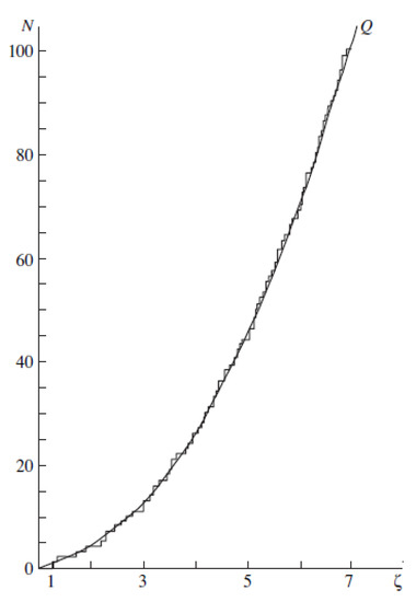
Figure 3. The number of levels with $ϵ<-m$ for the potential of the model II, cf. [5]. The stepwise broken line represents a numerical solution of the Dirac equation, while the curve Q was computed according to the semiclassical Equation (68).

4.6. Energy of Single-Particle Levels at $ϵ<-m$

4.6.1. Energy Spectrum for $|ϵ|-m\ll m$

Expand the effective potential in $m+ϵ$, cf. [3]:

$$U_{\mathrm{ef}}(r,ϵ)=\sum _{n=0}^{\infty }{(m+ϵ)}^n{u}_n\left(r\right),$$

(69)

where $U_{\mathrm{ef}}(r,ϵ)$ can be taken following Equation (21). Here, $u_0\left(r\right)=U_{\mathrm{ef}}(r,ϵ=-m)$. For $n\ge 1$,

$$u_n=\frac{V}{m^n}{\delta }_{n1}+\frac{1}{m{V}^n}\left[-\frac{V^{″}}{4V}+\frac{3(n+1)}{8}{\left(\frac{V^{\prime }}{V}\right)}^2+\frac{\kappa V^{\prime }}{2rV}\right],$$

(70)

where ${\delta }_{n1}$ is the Kronecker symbol.

The energy of the levels is found from the Bohr–Sommerfeld quantization condition

$${\int }_0^{r_{-}}\sqrt{-2m{u}_0}dr+(m+ϵ){\int }_0^{r_{-}}\sqrt{-2u_1}dr+O({(1+ϵ/m)}^{3/2})=(n_r+{\gamma }^{\prime })\pi .$$

(71)

As before, $\gamma =3/4$ for levels with $\kappa =-1$ and $\gamma =1/2$ for $\kappa \ne -1$. With the help of (71) we find

$$ϵ=-m+\beta ({\zeta }_{\mathrm{cr}}-\zeta )+...,$$

(72)

$$\beta =f_2/f_1,f_1={\int }_0^{r_{-}}\sqrt{-2m^2{u}_1}dr,f_2={\int }_0^{r_{-}}\frac{\zeta f^2/\left(m{R}_{\mathrm{nucl}}\right)-f}{\sqrt{-2u_0/m}{R}_{\mathrm{nucl}}}dr.$$

A comparison of numerical calculation done following these expressions with that for the exact Dirac equation again shows a good agreement. Note that the value $\beta$ determines the threshold behavior of the probability of the production of positrons.

4.6.2. Energy Spectrum for $|ϵ|\ll -m$

This spectrum has been found in [5]. For $\zeta \gg {\zeta }_{\mathrm{cr}}$, many levels have energies $|ϵ|\ll -m$. In this case, as follows from Equation (21) and (22), the terms $\propto \kappa$ in the centrifugal potential and in the spin term cancel each other. Approximately, we have

$$p^{*}\left(r\right)\simeq {[{(ϵ-V)}^2-{\kappa }^2/r^2]}^{1/2}.$$

(73)

For $k=\sqrt{{ϵ}^2-m^2}<\zeta /R_{\mathrm{nucl}}$, the turning point $r_{-}$ lies outside the nucleus, $r_{-}>R_{\mathrm{nucl}}$. Employing the Bohr–Sommerfeld quantization condition, we get

$$\begin{array}{cc}& k_n\simeq |{ϵ}_n|=c_0\zeta R_{\mathrm{nucl}}^{-1}{e}^{-n\pi /\zeta }=\zeta R_{\mathrm{nucl}}^{-1}{e}^{-(n-n_{*})\pi /\zeta },n>n_{*},\\ & c_0=\exp ({\int }_0^{1}f\left(x\right)dx-1),n_{*}=\zeta {\pi }^{-1}({\int }_0^{1}f\left(x\right)dx-1).\end{array}$$

(74)

For deeper levels, $k>\zeta R_{\mathrm{nucl}}^{-1}$, classically permitted region $r_0<r<r_{-}$ is completely inside the nucleus. Thereby, the spectrum is entirely determined by the expression for $f\left(x\right)$:

$$k_n=\zeta R_{\mathrm{nucl}}^{-1}f\left({\mathsf{\Xi }}_n\right),1\ll n\ll n_{*},$$

(75)

where ${\mathsf{\Xi }}_n$ is the root of equation

$${\int }_0^{\mathsf{\Xi }}f\left(x\right)dx-\mathsf{\Xi }f\left(\mathsf{\Xi }\right)=n\pi /\zeta .$$

(76)

For example, for the model II at $1\ll n\ll n_{*}$, we have

$$k_n=\frac{\zeta }{2R_{\mathrm{nucl}}}\left[3-{(n/n_{*})}^{2/3}\right],n_{*}=\frac{\zeta }{3\pi }.$$

(77)

From these expressions, it is easy to find expression for the level density $dn/dϵ$. For model II, we find

$$dn/dϵ=C{y}^{-1},\mathrm{for}0<y<1$$

(78)

and

$$dn/dϵ=C{(3-2y)}^{1/2},\mathrm{for},1<y<3/2$$

(79)

for $y=k{R}_{\mathrm{nucl}}/\zeta$, $C=const$. From here, we see the accumulation of levels toward the boundary $ϵ=-m$ ($k\to 0$).

For levels with arbitrary angular momenta the “Coulomb” part of the spectrum gets the form

$${ϵ}_{n\kappa }=-\zeta R_{\mathrm{nucl}}^{-1}c\left(\rho \right)\exp (-n\pi /\tilde{g}),$$

(80)

where $\rho =|\kappa |/\zeta$, $0<\rho <1$. Pre-exponential factor

$$c\left(\rho \right)=\exp \left[ln\left(2{\left(e\rho \right)}^{-1}(1-{\rho }^2)\right)-{(1-{\rho }^2)}^{-1/2}\mathrm{Arth}{(1-{\rho }^2)}^{1/2}+h\left(\rho \right)\right],$$

(81)

where $h\left(\rho \right)$ that is given by Equation (65) depends on the $f\left(x\right)$, $e=2.718...$ is the Euler number. The function $c\left(\rho \right)$ monotonically decreases with increase of $\rho$ from 1 for model I and from $\simeq 1.4$ for model II at $\rho =0$ up to zero for $\rho =1$ in both models.

Equation (80) is obtained at the condition that the turning point $r_{-}$ lies inside the nucleus. The condition of applicability of Equation (80) is $\tilde{g}/\pi \ll n<n_{\kappa }$. Because $n_{\kappa }\simeq (\tilde{g}/\pi )ln(\zeta /R_{\mathrm{nucl}})$, then, due to large values of the logarithm, this equation describes most of the levels crossed the boundary $ϵ<-m$.

The exponential dependence of ${ϵ}_n$ on n and the accumulation of levels near $ϵ=-m$, as follows from Equations (74) and (80), are related to the fact that $U_{\mathrm{ef}}\simeq -{\tilde{g}}^2/r^2$ for $r\to 0$. If R was zero, the electrons would collapse to the center. The spectrum of the Schrödinger equation in such a potential behaves as [89],

$$E_n=E_0{e}^{-2\pi n/\tilde{g}},$$

(82)

where $E_0$ is the energy of the lowest level. In our case, $E\simeq {ϵ}^2/2m$, and thereby we recover Equation (80) for $c\left(\rho \right)=1$.

4.7. Exponential Estimate of Probability of Spontaneous Production of Positrons

Because, following Dirac the process of the production of $e^{-}{e}^{+}$ pairs can be treated as the penetration of electrons of the lower continuum into the upper continuum through the classically forbidden region ($p^2<0$), the probability of this process is, as in case of spinless particles, determined by Equation (5). Equivalently, one can find the coefficient of transmission of the barrier in the effective potential or find semiclassical asymptotic of the functions G and F for $r\to \infty$. This single-particle picture is distorted with a deepening of the level and with the increase of the number of levels crossed the boundary $ϵ=-m$. We may use Equations (20)–(22) while taking the Langer correction into account, which improves the application of semiclassical expressions.

In the threshold region of positron energies setting $ϵ\simeq -m$ in the expression for the spin term $U_s$, we obtain

$$p^{*2}\left(r\right)\simeq {(ϵ-V)}^2-m^2-{\kappa }^2/r^2,$$

(83)

cf. with Equation (73) we have used for a description of the very deep levels. In case of the Coulomb field $V=-\zeta /r$, replacing (83) in (5), we obtain

$$W\sim \exp \left[-2\pi \zeta \left(\frac{{(m^2+k^2)}^{1/2}}{k}-{(1-{\rho }^2)}^{1/2}\right)\right],\rho =\kappa /\zeta ,k=\sqrt{{ϵ}^2-m^2}\ll m,$$

(84)

that coincides with the asymptotic of the exact solution of the Coulomb problem.

4.8. Critical Charge of Nucleus for Muon

For the electron, one has $R_{\mathrm{nucl}}\ll 1/m$, since $1/m\simeq 386$ fm and $R_{\mathrm{nucl}}\simeq r_0{A}^{1/3}\simeq A^{1/3}/m_{\pi }$, $m_{\pi }\simeq 280m$. For muon $R_{\mathrm{nucl}}\gg 1/m_{\mu }$, $m_{\mu }\simeq 207m_e$.

In order to find the critical charge for the muon, ${\zeta }_{\mathrm{cr}}^{\mu }$, when ${\mu }^{-}$ level reaches $ϵ=-m_{\mu }$, we continue to apply the semiclassical approximation. For the model I, the turning point lies outside the nucleus. Let us expand $U_{\mathrm{ef}}(r,ϵ)$ near the turning point. Using Equation (54), after the replacement $r_{-}\to r_0$, and matching solutions $G^{\prime }/G$ at $r=R_{\mathrm{nucl}}$, we find [3]:

$$\frac{{\mathrm{A}\mathrm{i}}^{\prime }\left(0\right)}{\mathrm{A}\mathrm{i}\left(0\right)}\frac{2}{{\zeta }^{1/3}}\simeq \frac{\beta \mathrm{ctg}\beta }{m_{\mu }{R}_{\mathrm{nucl}}},\beta =\sqrt{\zeta (\zeta -2R_{\mathrm{nucl}}{m}_{\mu })}$$

(85)

for the $ns$ level. From here follows

$${\zeta }_{\mathrm{cr}}^{\mu }\simeq 2R{m}_{\mu }+\frac{{\left(n\pi \right)}^2}{2R_{\mathrm{nucl}}{m}_{\mu }}(1+a{\left(R_{\mathrm{nucl}}{m}_{\mu }\right)}^{-2/3}+...),a=-2^{4/3}{3}^{-5/6}\pi {\mathsf{\Gamma }}^2(2/3),$$

(86)

that coincides with expression, which follows from the direct solution of the Dirac equation at $ϵ=-m_{\mu }$. In the model II we obtain ${\zeta }_{\mathrm{cr}}^{\mu }\simeq 16.7$ that corresponds to $Z_{\mathrm{cr}}^{\mu }\simeq 2300$, and in the model I, respectively $Z_{\mathrm{cr}}^{\mu }\simeq 3700$.

5. Semiclassical Approximation to System of Linear Dirac Equations

5.1. Semiclassical Wave Functions

Let us apply semiclassical expansion to Equation (18), cf. [7]. The parameter of expansion $\tilde{\lambda }/l$ is $\propto \hslash$, where l is the typical length for the change of the potential. We present

$$\psi =\varphi e^{{\int }^{r}ydr},$$

(87)

$$y\left(r\right)=\frac{1}{\hslash }{y}_{-1}\left(r\right)+y_0\left(r\right)+\dots ,\varphi =\sum _{n=0}^{\infty }{\hslash }^n{\varphi }^{\left(n\right)},$$

(88)

and arrive at the chain of equations for $y_n$ and ${\varphi }^{\left(n\right)}$:

$$(\widehat{D}-y_{-1}){\varphi }^{\left(0\right)}=0,(\widehat{D}-y_{-1}){\varphi }^{\left(1\right)}={\varphi }_r^{\left(0\right)\prime }+y_0{\varphi }^{\left(0\right)},\dots$$

(89)

One usually restricts expansion by consideration of first two terms. Because semiclassical series is an asymptotic one, retaining of too many terms may worsen the convergence of the series to the exact solution.

In order the system of homogeneous Equation (89) to have nontrivial solution, $y_{-1}\left(r\right)$ should be an eigenvalue and ${\varphi }^{\left(0\right)}\equiv {\varphi }_i$, $i=1,2$, the eigenfunction of one of two-component eigenvectors of the matrix $\widehat{D}\left(r\right)$. From the condition $\det \widehat{D}=0$, we get

$$y_{-1}\equiv {\lambda }_i=\pm i\sqrt{{(ϵ-V)}^2-m^2-{\tilde{\kappa }}^2/r^2}\equiv \pm q.$$

(90)

Replacing $y_{-1}$ back to Equation (89), we obtain

$${\varphi }_i=A\left(\begin{array}{c}m+ϵ-V\\ {\lambda }_i+\kappa /r\end{array}\right)=A_1\left(\begin{array}{c}{\lambda }_i-\kappa /r\\ m-ϵ+V\end{array}\right),$$

(91)

where A and $A_1$ are normalization constants.

Because the matrix $\widehat{D}$ is not symmetrical, besides the right-hand eigenvectors ${\varphi }_i$, we should introduce the left-hand eigenvectors ${\tilde{\varphi }}_i$:

$$\begin{array}{cc}& (\widehat{D}-{\lambda }_i){\varphi }_i={\tilde{\varphi }}_i(\widehat{D}-{\lambda }_i)=0,\\ & {\tilde{\varphi }}_i=A(m-ϵ+V,{\lambda }_i+\kappa /r)=A_1({\lambda }_i-\kappa /r,m-ϵ-V).\end{array}$$

(92)

Note that the left eigenvectors do not coincide with transposed right eigenvectors (${\tilde{\varphi }}_i\ne {\varphi }_i^T$) and the left-hand and right-hand vectors are mutually orthogonal,

$$({\tilde{\varphi }}_i,{\varphi }_j)=\sum _{\alpha =1}^2{({\tilde{\varphi }}_i)}_{\alpha }{\left({\varphi }_j\right)}_{\alpha }\sim {\delta }_{ij}.$$

(93)

To determine $y_0$, let us put ${\varphi }^{\left(0\right)}={\varphi }_i$ in Equation (89) and multiply both sides of equation from the left by ${\tilde{\varphi }}_i$. As follows from the first Equation (92), the term with ${\varphi }^{\left(1\right)}$ vanishes, and we obtain

$$y_0=-({\tilde{\varphi }}_i,{\varphi }_i^{\prime })/({\tilde{\varphi }}_i,{\varphi }_i).$$

(94)

Further calculations entail no difficulty, cf. [7,90]. The resulting wave functions of the quasistationary state with energy $ϵ<-m$ in the region of classically permitted motion $r_0<r<r_{-}$ to have the form:

$$\begin{array}{cc}& G=C_1{\left[\frac{ϵ+m-V}{p}\right]}^{1/2}\sin {\theta }_1,F=\mathrm{sgn}\kappa ·C_1{\left[\frac{ϵ-m-V}{p}\right]}^{1/2}\sin {\theta }_2,\\ & p=-iq=\sqrt{{(ϵ-V)}^2-m^2-\frac{{\kappa }^2}{r^2}},{\theta }_1={\int }_r{{}_0}^r(p+\frac{\kappa w}{pr})dr+\pi /4,\\ & {\theta }_2={\int }_{r_0}^r(p+\frac{\kappa \tilde{w}}{pr})dr+\pi /4,w=\frac{1}{2}\left(\frac{V^{\prime }}{m+ϵ-V}-\frac{1}{r}\right),\tilde{w}=\frac{1}{2}\left(\frac{V^{\prime }}{m-ϵ+V}+\frac{1}{r}\right).\end{array}$$

(95)

Here, $C_1$ is normalization constant. As it was discussed, semiclassical wave functions can be normalized neglecting penetration of the particle into the classically forbidden regions $r<r_0$ and $r>r_{-}$, i.e., ${\int }_{r_0}^{r_{-}}(G^2+F^2)dr=1$. Thus, we find

$$C_1={\left[{\int }_{r_0}^{r_{-}}\frac{ϵ-V}{p}dr\right]}^{-1/2}={\left(\frac{2}{T}\right)}^{1/2},$$

(96)

where T is the period of the particle motion in the classically allowed region.

In the sub-barrier region $r_{-}<r<r_{+}$, where $p^2<0, p=iq$ and q, $y_{-1}$ and $y_0$ are real, wave functions attenuate exponentially with increasing r. The resulting expressions have different forms in dependence on the sign of $\kappa$. For $\kappa <0$, i.e., for $\kappa =-1$, we have

$$\psi =\left(\begin{array}{c}G\\ F\end{array}\right)=C_{2-}{\left(Qq\right)}^{-1/2}\exp \left[-{\int }_{r_{-}}^r\left(q-\frac{V^{\prime }m}{2Qq}\right)dr\right]\left(\begin{array}{c}m+ϵ-V\\ -Q\end{array}\right)$$

(97)

with $Q=q-\kappa /r$.

For $\kappa >0$, we have

$$\begin{array}{c}\hfill \psi =C_{2+}{\left(Qq\right)}^{-1/2}\exp \left[-{\int }_{r_{-}}^r\left(q+\frac{V^{\prime }m}{2Qq}\right)dr\right]\left(\begin{array}{c}-Q\\ m-ϵ+V\end{array}\right)\end{array}$$

(98)

with $Q=q+\kappa /r$, $C_{2\pm }$ are normalization constants.

In the region $r>r_{+}$, the quasistationary state describes outgoing positron and represents a diverging wave. For $\kappa <0$:

$$\begin{array}{c}\hfill \psi =i{C}_{3-}{\left(Pp\right)}^{-1/2}\exp \left[-{\int }_{r_{+}}^r\left(ip-\frac{V^{\prime }m}{2Pp}\right)dr\right]\left(\begin{array}{c}m+ϵ-V\\ iP\end{array}\right)\end{array}$$

(99)

with $P=p-i\kappa /r$. The flux of particles moving to infinity is then given by $\mathsf{\Gamma }=\lim \mathrm{Im}\left(F^{*}G\right)$ at $r\to \infty$.

For $\kappa >0$:

$$\begin{array}{c}\hfill \psi =i{C}_{3+}{\left(Pp\right)}^{-1/2}\exp \left[-{\int }_{r_{+}}^r\left(ip+\frac{V^{\prime }m}{2Pp}\right)dr\right]\left(\begin{array}{c}iP\\ m-ϵ+V\end{array}\right)\end{array}$$

(100)

with $P=p+i\kappa /r$. $C_{2\pm }$ are normalization constants.

The obtained formulas are valid for all r, except regions $\delta r\propto 1/{\zeta }^{2/3}$ near the turning points. The usual procedure is employed to match semiclassical solutions. The solution is either expressed in terms of an Airy function or one may use the Zwaan’s method. Consequently, we have

$$\begin{array}{ccc}& C_{2\pm }& =-i{C}_{3\pm }\hfill \\ & =& -\frac{\mathrm{sgn}\kappa }{2}{C}_{1}m{\left[\frac{|\kappa |}{m{r}_{-}+{({\kappa }^2+r_{-}^2{m}^2)}^{1/2}}\right]}^{-\mathrm{sgn}\kappa /2}\exp \left[-{\int }_{r_{-}}^{r_{+}}\left(q+\mathrm{sgn}\kappa \frac{V^{\prime }m}{2Qq}\right)dr\right].\hfill \end{array}$$

(101)

Note that the effective potential, which we have used in (20), can be presented while employing function w that appeared in (95):

$$U_{\mathrm{ef}}=-\frac{V^2}{2m}+\frac{ϵV}{m}+\frac{\kappa (\kappa +1)}{2r^{2}m}-\frac{\kappa }{rm}w+\frac{1}{2m}(w^{\prime }+w^2+\frac{w}{r}).$$

(102)

The terms in Equation (102), which contain the function w, are due to the electron spin. For $|V|\gg m$, they are small compared to the first three terms. Subsequently, the expression for the effective potential takes the same form as for a scalar particle. At the turning points $r_{-}$ and $r_{+}$, the effective potential is not singular.

The action becomes

$$S={\int }^{r}dr\sqrt{2m(E-U_{\mathrm{ef}})}={\int }^{r}dr{\left[p+\frac{2\kappa w}{pr}-m^{-1}(w^{\prime }+w^2+\frac{w}{r})\right]}^{1/2}.$$

(103)

Expanding S in $1/\zeta \ll 1$, we obtain

$$S={\int }^{r}dr\left[p+\frac{\kappa w}{pr}+O(m/{\zeta }^2)\right],$$

(104)

that coincides with Equations (95)–(100), which we have derived in this section.

Using Equations (95)–(100) for $ϵ=-m$, we obtain

$$\overline{r}=\frac{3({\zeta }^2-{\kappa }^2+1/4)({\zeta }^2+2{\kappa }^2/3-5\kappa /3+1)}{10\zeta ({\zeta }^2+({\kappa }^2-3\kappa /2+1/2)/2)}.$$

(105)

This expression yields $\overline{r}=0.301/m$ for the ground-state level, whereas the exact result gives $0.303/m$. For $\zeta \gg |\kappa |\gg 1$, result (105) coincides with that follows from (56).

5.2. Nonrelativistic Limit

To be specific consider case $\kappa <0$ and the classically allowed region. Introducing a nonrelativistic energy $\widetilde{ϵ}=ϵ-m$ and the variable $\tilde{q}={(q^2+\kappa /r^2)}^{1/2}\simeq q+\frac{\kappa }{2q{r}^2}$, let us transform the factor in exponent (97) as

$${\int }_{r_{-}}^{r}dr\left(q-\frac{V^{\prime }m}{2Qq}\right)={\int }_{r_{-}}^{r}dr\left[\tilde{q}-\frac{1}{2q}(V^{\prime }/Q+\kappa /r^2)\right]={\int }_{r_{-}}^{r}dr\left[\tilde{q}-\frac{1}{2}{(lnQ)}^{\prime }\right],$$

(106)

where $Q=q-\kappa /r$. The latter term in the integral cancels with the pre-exponential factor $Q^{-1/2}$. Now let us take into account that $\kappa (1+\kappa )=l(1+l)$. Subsequently, we have

$$\tilde{q}\left(r\right)={\left[2m(-\widetilde{ϵ}+V\left(r\right)-l(l+1)/\left(2m{r}^2\right)\right]}^{1/2},G\left(r\right)=\frac{C}{{\tilde{q}}^{1/2}\left(r\right)}\exp (-{\int }_{r_{-}}^{r}dr\tilde{q}\left(r\right),$$

(107)

where $C=const$ that reproduces the Schrödinger wave function in this region. Note that $\tilde{q}\left(r\right)$ enters not $\kappa =\mp (j+1/2)$, but orbital moment l. We formally considered case $\kappa <0$ just to be specific. Case $\kappa >0$ is considered similarly. Additionally, note that, for $\kappa \ne -1$, one should add to $\tilde{q}\left(r\right)$ the Langer correction.

5.3. Bohr-Sommerfeld Quantization Rule

From (97), (98) we derive [7],

$${\int }_{r_0}^{r_{-}}dr(p+\frac{\kappa w}{pr})=(n+{\gamma }^{\prime }).$$

(108)

As we have mentioned, value ${\gamma }^{\prime }$ depends on the fact does $r_0$ lie inside the nucleus or outside it. In the latter case, ${\gamma }^{\prime }=1/2$ for $\kappa \ne -1$ and ${\gamma }^{\prime }=3/4$ for $\kappa =-1$.

Equation (108) determines the real part of the energy ${ϵ}_{n\kappa }$. It differs from the ordinary Bohr–Sommerfeld rule used in nonrelativistic quantum mechanics by expression for relativistic momentum $p\left(r\right)$ and by the term $\propto w$ appeared due to the spin–orbital interaction. Taking into account of the term $\propto w$ is legitimate within semiclassical scheme. Let us show it on an example of the Coulomb field $V=-\zeta /r$. Subsequently, $w\left(r\right)=-\frac{m+ϵ}{2(\zeta +(m+ϵ\left)r\right)}$ and $p\left(r\right)$ is determined by Equation (95). For $r_0<r<r_{-}$, the momentum $p\left(r\right)\sim \tilde{g}/r$ and the ratio $|\frac{\kappa w}{p^{2}r}|\sim |\kappa {\tilde{g}}^{-2}rw|\sim |\kappa |/{\zeta }^2$ for deep levels. Because semiclassical approximation for wave functions is valid up to $1/{\zeta }^2$, the second term in the integral (108) should be retained in the case of deep levels $|ϵ|\gg m$ for $|\kappa |\gg 1$, but it can be dropped for $|\kappa |\sim 1$. For $ϵ=-m$, we have $w=0$.

Note that the results of calculations performed with the help of the quantization rules (50) and (108) differ only in correction terms. For instance, from (108), we derive exactly the same electron energy spectrum as that given by Equations (80) and (81), with the help of the quantization rule in the form (50).

5.4. Probability of Spontaneous Production of Positrons

Let us calculate the probability of spontaneous production of positrons, $\mathsf{\Gamma }=-2\mathrm{Im}ϵ$. Replacing (99), (100) in (40), we find

$$\mathsf{\Gamma }={\mathsf{\Gamma }}_0{e}^{-2{\int }_{r_{-}}^{r_{+}}q\left(r\right)dr},{\mathsf{\Gamma }}_0=T^{-1}{e}^{2\kappa \mathrm{Pr}{\int }_{r_{-}}^{r_{+}}wdr/\left(qr\right)}.$$

(109)

The last integral is understood in the sense of the principal value, being denoted as $\mathrm{Pr}$, due to singularity at the point where $V\left(r\right)=m+ϵ$.

In the nonrelativistic limit, the value ${\mathsf{\Gamma }}_0=1/T$ has the meaning of the number of impacts per unit time of the particle (localized inside the region $r_0<r<r_{-}$) against the potential barrier at $r=r_{-}$, and the exponential is the probability of the penetration of the barrier in each impact. The allowance for the relativistic effects and the spin change the expression for the period of the oscillations and add to (109) a factor depending on the sign of $\kappa$.

While taking into account that in the region of the barrier V is the purely Coulomb field, for $w=0$ all of the integrals are calculated exactly:

$$\begin{array}{cc}& \mathsf{\Gamma }={\mathsf{\Gamma }}_0\exp \left[-2\pi \zeta \left({(m^2+k^2)}^{1/2}/k-{(1-{\rho }^2)}^{1/2}\right)\right],\\ & 1/{\mathsf{\Gamma }}_0=\frac{2\zeta }{k^2}\left[{(1-{\rho }^2)}^{1/2}{(m^2+k^2)}^{1/2}-\frac{m^2}{k}\mathrm{Arth}\left(k{\left(\frac{1-{\rho }^2}{m^2+k^2}\right)}^{1/2}\right)\right].\end{array}$$

(110)

For the positron momentum $k=\sqrt{{ϵ}^2-m^2}\to 0$, we have ${\mathsf{\Gamma }}_0=c_1=3/[2\zeta {(1-{\rho }^2)}^{1/2}(2+{\rho }^2)]$, and, for $k\to \infty$, we have ${\mathsf{\Gamma }}_0=c_{2}k=k/[2\zeta {(1-{\rho }^2)}^{1/2}]$. For $k\ll {\zeta }^{1/2}m$ the width $\mathsf{\Gamma }$ is exponentially small for any $\kappa$. For $|\kappa |\gg {(\zeta /\pi )}^{1/2}$ expression simplifies as

$$\mathsf{\Gamma }\simeq k{\left[2\zeta (1-{\rho }^2)\right]}^{-1/2}\exp [-2\pi \zeta (1-{(1-{\rho }^2)}^{1/2})].$$

(111)

For $|\kappa |\lesssim {\kappa }_0={(\zeta /\pi )}^{1/2}$, the exponential factor in $\mathsf{\Gamma }$ becomes of the order of unity, and the semiclassical approximation becomes invalid. Note that ${\kappa }_0/{\kappa }_{max}=1/\sqrt{\pi \zeta }$. Therefore, a number of levels diffused in the continuum, for which $\mathsf{\Gamma }$ is not exponentially small, is tiny for $\zeta \gg 1$.

5.5. Semiclassical Method for Noncentral Potentials Obeying System of Linear Dirac Equations

We described the spectrum of the quasistationary levels in the lower continuum for a spherical nucleus with the charge $Z>Z_{\mathrm{cr}}$. The results can be generalized to the case, when the potential does not obey spherical symmetry [7]. Let us present the Dirac equation as

$$-i(\widehat{\overrightarrow{\alpha }}\nabla )\psi ={\hslash }^{-1}\widehat{D}\psi ,\widehat{D}=ϵ-m\widehat{\beta }-V\left(\overrightarrow{r}\right),$$

(112)

where $\widehat{\overrightarrow{\alpha }}={\gamma }^0\overrightarrow{\gamma }$, $\widehat{\beta }={\gamma }^0$ are Dirac matrices, and we recovered dependence on ℏ. Let us present bispinor $\psi$ as $\psi =\varphi e^{i\sigma }$ and expand real quantities $\varphi$ and $\sigma$ in the parameter that is proportional to ℏ:

$$\sigma ={\hslash }^{-1}{\sigma }_{-1}+{\sigma }_0+\dots ,\varphi ={\varphi }^{\left(0\right)}+\hslash {\varphi }^{\left(1\right)}+\dots$$

(113)

Replacing these series to Equation (112), we obtain the chain of equations

$$\begin{array}{cc}& [\widehat{D}-(\widehat{\overrightarrow{\alpha }}\nabla {\sigma }_{-1})]{\varphi }^{\left(0\right)}=0,\\ & [\widehat{D}-(\widehat{\overrightarrow{\alpha }}\nabla {\sigma }_{-1})]{\varphi }^{\left(1\right)}=\widehat{\overrightarrow{\alpha }}\nabla ){\varphi }^{\left(0\right)}+(\widehat{\overrightarrow{\alpha }}\nabla {\sigma }_0){\varphi }^{\left(0\right)},\dots \end{array}$$

(114)

The condition of existence of a nontrivial solution ${\varphi }^{\left(0\right)}$,

$$\det [\widehat{D}-(\widehat{\overrightarrow{\alpha }}\nabla {\sigma }_{-1})]=0,$$

(115)

results in the Hamilton–Jacobi equation

$${(\nabla {\sigma }_{-1})}^2={(ϵ-V)}^2-m^2.$$

(116)

In difference with the spherically-symmetric case, the matrix

$$\widehat{D}-\widehat{\overrightarrow{\alpha }}\nabla {\sigma }_{-1}=ϵ-V\left(\overrightarrow{r}\right)-m\widehat{\beta }-\widehat{\overrightarrow{\alpha }}\nabla S$$

(117)

is Hermitian; therefore, its left-hand, ${\tilde{\varphi }}_i$, and right-hand, ${\varphi }_i$, eigenvectors are Hermitian conjugates, ${\tilde{\varphi }}_i={\varphi }_i^{†}$, and

$$(\widehat{D}-\widehat{\overrightarrow{\alpha }}\nabla S){\varphi }_i={\varphi }_i^{†}(\widehat{D}-\widehat{\overrightarrow{\alpha }}\nabla S)=0,i=1,2,3,4.$$

(118)

With the help of this equation, from (114), we find a system of equations for ${\sigma }_0$,

$${\varphi }_i^{†}(\widehat{\overrightarrow{\alpha }}\nabla {\sigma }_0){\varphi }_j=-{\varphi }_i^{†}\widehat{\overrightarrow{\alpha }}\nabla {\varphi }_j.$$

(119)

Bispinors ${\varphi }_i$ are found by diagonalizing the matrix $\widehat{D}-\widehat{\overrightarrow{\alpha }}\nabla S$, so that the right-hand side of Equation (119) contains known quantities. Determining from this equation ${\sigma }_0$, we obtain the quasiclassical solution of the Dirac equation

$$\psi ={\varphi }_i\exp ({\hslash }^{-1}{\sigma }_{-1}+{\sigma }_0).$$

(120)

In practice, the calculation of the functions ${\sigma }_{-1}$ and ${\sigma }_0$ for noncentral potentials is a complicated mathematical problem requiring the solution of first-order differential equations in partial derivatives. In contrast to the case when V is spherically symmetric, in general case the result is not expressed in quadratures. If a parameter of a “non-sphericity” is small, then one may develop a perturbation theory.

6. Spontaneous Production of Positrons in Heavy-Ion Collisions

6.1. Approach to the Problem

The minimal distance between colliding nuclei with charges $Z_1$ and $Z_2$ is as follows [18,91],

$$R_{\min }={(Z_1+Z_2)}^2{e}^2/\left(2E_{\mathrm{c}.\mathrm{m}.}\right)+\sqrt{{(Z_1+Z_2)}^2{e}^2/{\left(2E_{\mathrm{c}.\mathrm{m}.}\right)}^2+b^2},$$

where $E_{\mathrm{c}.\mathrm{m}.}$ is the kinetic energy of colliding nuclei in c.m. reference frame, b is the impact parameter. In order the energy of the electron, ${ϵ}_{1\mathrm{s}}$, in the quasi-molecule would become $<-m$ the colliding heavy nuclei should reach distances $|{\overrightarrow{r}}_1-{\overrightarrow{r}}_2|=R<R_{\mathrm{cr}}$, where $R_{\mathrm{cr}}\simeq 33$ fm for central U+U collisions, see below. Thus, $R_{\mathrm{cr}}$ is approximately twice larger than $2R_{\mathrm{nucl}}$, where $R_{\mathrm{nucl}}\simeq 1.2A^{1/3}$ fm is the radius of the single nucleus $\simeq 7$ fm. On the other hand, $R_{\mathrm{cr}}\ll {\overline{r}}_K\simeq 0.3{\zeta }_{\mathrm{cr}}$, where $\overline{r}$ is estimated using Equation (105). For U+U collisions, $R_{\mathrm{cr}}/{\overline{r}}_K\sim 0.2$. Nuclei move with the velocity $v_A\sim (0.025-0.07)$, cf. [18], whereas the electron of the K-shell has a typical velocity $v_e\simeq 1$. Thereby, one may use adiabatic approximation, i.e., we may use $ϵ\left(R\right(t\left)\right)$. Because $R_{\mathrm{cr}}/{\overline{r}}_K\sim 0.2\ll 1$, the anisotropy of the potential is not as large, and we may present

$$V\left(r\right)=-\left(\frac{Z_1{e}^2}{r_1}+\frac{Z_2{e}^2}{r_2}\right)=-\frac{Z{e}^2}{r}\left(1+\frac{R^2}{{\left(2r\right)}^2}{P}_2(cos\theta )+...\right),$$

(121)

where $Z=Z_1+Z_2$, ${\overrightarrow{r}}_{1,2}=|\overrightarrow{r}\pm \overrightarrow{R}/2|$, $P_2$ is the second Legendre polinomical, $R\left(t\right)$ is the distance between centers of nuclei. In the second equation and, further we for simplicity, consider the case $Z_1=Z_2$. Otherwise, odd-power terms appear in the expansion. In inclusive experiments, this anisotropy disappears due to the averaging. However for event-by-event collisions such terms may lead to the forward-backward anisotropy reflecting in some observable effects. In the first approximation in ${(R/2{\overline{r}}_K)}^2$, the problem is reduced to that we have considered above for the spherical nucleus with the charge $Z=Z_1+Z_2$. The effective nucleus radius now is $2R_{\mathrm{nucl}}$.

The process of the spontaneous production of positrons can also be described in adiabatic approximation, since, as we have argued, we may use that $ϵ\left(R\right(t\left)\right)$ and, since $1/\mathsf{\Gamma }\left(ϵ\left(R\left(t\right)\right)\right)\gg {\tau }_{\mathrm{col}}\gtrsim 2R_{\mathrm{cr}}/v_A$. The most serious experimental problem is to separate spontaneous production of positrons in the tunneling process from the frequency dependent processes also resulting in a production of positrons. For example, the parameter $2R_{\mathrm{nucl}}/R_{\mathrm{cr}}\sim (1/2-1/3)$ is not as small. Therefore, a serious competing time-dependent process is associated with an induced production of positrons occurring due to excitation of the nuclear levels, cf. [20,92] and the references therein. However, the difference between characteristics of the induced and spontaneous production of positrons is significant. The induced positron production exists in both subcritical and supercritical regimes. When the electron level crosses the boundary $ϵ=-m$, there appears a narrow energy-line in the positron spectrum owing to the switching on of the spontaneous positron production occurring in the tunneling process. Thus, there is a principal difference between the subcritical and the supercritical regimes that may help in the experimental identification of the spontaneous positron production.

Another effect is associated with the presence of a magnetic component of the field. First, an indication on presence of strong magnetic fields in heavy ion collisions was performed in [93]. For peripheral collisions of heavy ions at collision energies $\lesssim$ GeV$·A$ it yields $h\sim H_{\pi }{\left(Z{e}^6\right)}^{1/3}$ for $R\simeq A^{1/3}/m_{\pi }$, $v_A\sim 1$, $H_{\pi }=m_{\pi }^2/e$. More generally, replacing $1\to v_A\gamma$, $\gamma =1/\sqrt{1-v_A^2}$, we have

$$eh\sim Z{e}^2{v}_A\gamma /R^2.$$

(122)

For collisions with low energies $E\sim (5-10)$ MeV$·A$ of our interest here, it follows that $h\sim {10}^{15}$G, for $R\sim R_{cr}\simeq (30-50)$ fm, and $v_A\sim {10}^{-1}$, cf. also [94].

In the presence of a “weak” homogeneous magnetic field, the reduction of $Z_{\mathrm{cr}}$ in the case of the supercritical atom has been found by using the perturbation theory [95],

$${\zeta }_{\mathrm{cr}}\left(h\right)={\zeta }_{\mathrm{cr}}\left(0\right)-\frac{5{\pi }^2\mu }{6ln(1/R_{\mathrm{nucl}}^3)}\frac{h}{H_0},$$

(123)

$H_0=m^2/e\simeq 4.4·{10}^{13}$G, $\mu \simeq 1/3$ for $\zeta ={\zeta }_{\mathrm{cr}}$.

For strong fields, numerical evaluations [95], see also [19], yielded $Z_{\mathrm{cr}}=165$ for $h=H_0$, and $Z_{\mathrm{cr}}=96$ at $h={10}^2{H}_0$. For $h={10}^{18}$G, one gets $Z_{\mathrm{cr}}=41$. This effect appears because of the exact compensation of the diamagnetic and paramagnetic contributions to the ground state for the electron. Although these estimates are performed for the case of purely uniform static magnetic field, they show that a magnetic effect also should be carefully studied for the case of realistic time-space configuration of the field.

Below, I only focus on the description of the spontaneous production of positrons and, simplifying this consideration, I also ignore the mentioned magnetic effects.

6.2. Electron Energy as a Function of Distance between Nuclei

Usage of the Bohr–Sommerfeld quantization rule allows for considering the problem analytically [8], cf. [7]. From (19)–(21), taking into account of the Langer correction resulting in the replacement $p\to p^{*}$, we have

$$p^{*}\left(r\right)=\frac{F(r,ϵ)}{r},F(r,ϵ)={\left[({ϵ}^2-m^2)r^2+2ϵ\zeta r+\frac{\kappa +1}{\tilde{a}}-\frac{3}{4{\tilde{a}}^2}-{(\kappa +1/2)}^2+{\zeta }^2\right]}^{1/2},$$

(124)

where $\tilde{a}=1+r(m+ϵ)/\zeta$, $\zeta =Z{e}^2$, $Z=Z_1+Z_2$. Applying the quantization rule (50), first for $ϵ\ne -m$ and then for $ϵ=-m$, and subtracting one result from the other, we obtain

$${\int }_{R/2}^{r_{ϵ}}drF(r,ϵ)/r={\int }_{R_{\mathrm{cr}}/2}^{r_{-m}}drF(r,ϵ=-m)/r.$$

(125)

Here, $r_{ϵ}$ is the turning point for the given $ϵ$ and $r_{-m}$ is the turning point for $ϵ=-m$. I used that in integration over the regions $r<R/2$, $r<R_{\mathrm{cr}}/2$ dependence on $ϵ$ can be dropped, since at $|ϵ|\sim m$ of our interest, we have $|V|\gg |ϵ|$. Thereby, the specifics of the behavior $V\left(r\right)$ in the region $r<R_{\mathrm{cr}}/2$ almost does not affect the result. To be specific, we may use $V=const$ for $r<R_{\mathrm{cr}}/2$. Integrals undergo logarithmic diverge at the lower limit. After their regularization, the dependence on R and $R_{\mathrm{cr}}$ is separated in the explicit form:

$${\int }_0^{r_{ϵ}}dr[F(r,ϵ)-F(r,ϵ=-m)]/r+{\int }_{r_{-m}}^{r_{ϵ}}drF(r,ϵ=-m)/r=\tilde{g}ln\frac{R}{R_{\mathrm{cr}}}.$$

(126)

Integrals in (126) are calculated numerically. A comparison with the exact solution of two-center Dirac problem shows that the error of the semiclassical result does not exceed $0.1\%$. We can proceed further using that $r|m+ϵ|/\zeta <r_{ϵ}|m+ϵ|/\zeta \ll 1$ at least for $|ϵ|\sim m$ of our interest. Thereby, we expand $\tilde{a}$ in Equation (124) in the series of r. As the result, we find

$$\begin{array}{cc}& F(r,ϵ)={({\tilde{g}}^2+br+c{r}^2)}^{1/2},\\ & b=2ϵ\zeta -(\kappa -1/2)(m+ϵ)/\zeta ,c={ϵ}^2-m^2+(\kappa -5/4){(ϵ+m)}^2/{\zeta }^2.\end{array}$$

(127)

From (126) and (127), we obtain

$$\frac{R}{R_{\mathrm{cr}}}=-\frac{2\zeta }{b}\left(1+\frac{{\tilde{g}}^{2}c}{3b^2}+O\left(c^2\right)\right).$$

(128)

For $|ϵ+m|\ll m$, we find

$$ϵ=-m-\beta m(R-R_{\mathrm{cr}})/R_{\mathrm{cr}},\beta ={\left(1-\frac{\kappa -1/2}{2{\zeta }^2}-\frac{{\tilde{g}}^2}{3{\zeta }^2}\right)}^{-1}.$$

(129)

For U $+ U$ collisions for the ground-state level, we find $\zeta \simeq 1.343$ and $\beta \simeq 0.79$. The slope-parameter $\beta$ determines the probability of the production of positrons for $|ϵ+m|\ll m$. The semiclassical approximation reproduces the Z dependence of $\beta$ correctly, the difference with exact calculation done within solution of the two-center problem for the Dirac equation [96] is approximately (3–4)%.

Setting $c=0$ in Equation (128), we obtain a very simple and accurate result [6,7,8]:

$$ϵ\left(R\right)=ϵ(R/R_{\mathrm{cr}})=-m\frac{R_{\mathrm{cr}}/R-(\kappa -1/2)/\left(2{\zeta }^2\right)}{1-(\kappa -1/2)/\left(2{\zeta }^2\right)}.$$

(130)

The difference of this simple expression with exact solution of the two-center Dirac Equation [96] is less than (1–2)% already for $\zeta \to 1$ when the parameter of applicability of the semiclassical approximation is $1$. Such an accuracy is sufficient; therefore, here I do not present a more accurate semiclassical expression [7] obtained without using expansion in $c^2$, which has still higher accuracy. It may be curious to notice that, when in 1976 I showed the result (130) to Vladimir Stepanovich Popov, he did not believe in it, saying that one of his collaborators during a year is trying to solve the Dirac equation for the two-center problem numerically on ITEP big computer and, yet, only obtained the result for $\zeta =1$. He took the slide rule (that time there were no PCs) and confirmed that for $\zeta =1$ the whole curve (130) fully coincides with the result of the exact numerical calculation. Because the criterion of applicability of the semiclassical approximation for the ground state is ${\tilde{g}}_0\gg 1$, it became clear that, for $\zeta >1$, the accuracy of approximate solution (130) should at least not be worse than in case $\zeta =1$.

Subsequently, the result (130) was reflected in our publications [6,7]. Result (130) is shown in Figure 4. For $\zeta =1.343$, $\kappa =-1$, we get $-ϵ(R/R_{\mathrm{cr}})=0.705(R_{\mathrm{cr}}/R)+0.295$.

Figure 4. Solution $ϵ(R/R_{\mathrm{cr}})$ of Equation (130) for various values of the parameter $\zeta$.

The expression for the critical distance between nuclei, $R_{\mathrm{cr}}$, can be found from Equation (62) for a spherical nucleus after replacement of the nucleus radius $R_{\mathrm{nucl}}$ by $R/2$, where, now, R is the distance between nuclei and $Z\to Z_1+Z_2$. Consequently, we find

$$R_{\mathrm{cr}}=\frac{4{\tilde{g}}^2}{\zeta m}{\left[\exp \left(\frac{\pi (n+{\gamma }_1)-\tilde{\gamma }}{\tilde{g}}+2\right)+2\right]}^{-1}.$$

(131)

For the case of U+U collisions, in the model I that we obtain $R_{\mathrm{cr}}\simeq 33$ fm, whereas exact solution of the Dirac equation [96] yields $R_{\mathrm{cr}}\simeq 34.3$ fm.

6.3. Tunneling in the Two-Center Problem. Angular Distribution of Positrons

The potential of the system of two nuclei (121) contains, at $r\gg R$, a quadrupole correction. In the sub-barrier region, the correction is $\lesssim {(R_{\mathrm{cr}}/\left(2r_{-}\right))}^2\lesssim {10}^{-2}$. Therefore, the problem is reduced to the calculation of the penetrability of a three-dimensional barrier that only differs little from a spherically symmetrical one. Thus, we may use expansion

$$V=V_0+m^2{R}^2{V}_1,S=S_0+m^2{R}^2{S}_1.$$

(132)

We substitute these expressions to the Hamilton–Jacobi equation and obtain

$$\begin{array}{cc}& {(\nabla S_0)}^2=2m(E-U_0),\nabla S_0\nabla S_1=-U_1,\\ & U_0\left(r\right)=-\left(\frac{{\zeta }^2}{2r^{2}m}+\frac{\zeta ϵ}{rm}\right),U_1\left(r\right)=-\frac{\zeta }{4r^3{m}^2}\left(ϵ+\frac{\zeta }{r}\right)P_2(cos\theta ).\end{array}$$

(133)

The first equation is easily integrated, resulting in

$$S_0(r,\theta )={\int }^{r}pdr+\kappa \theta .$$

(134)

Taking the first term into account leads to exponential term in Equation (110). Second term in (134) is due to anisotropy of the potential.

Equation for $S_1$ in the under-barrier region $r_{-}<r<r_{+}$ gets the form

$$iq\frac{\partial S_1}{\partial r}+\frac{\kappa }{r^2}\frac{\partial S_1}{\partial \theta }=-U_1(r,\theta ),p=iq,$$

(135)

and it is solved by the method of separation of the variables. Supposing

$$r^2{U}_1(r,\theta )=u\left(r\right)(\frac{3}{4}cos\left(2\theta \right)+\frac{1}{4})$$

(136)

and taking into account the boundary condition $\mathrm{Im}{S}_1(r_{-},\theta )=0$, for $r=r_{+}$ we obtain

$$\begin{array}{cc}& \mathrm{Im}{S}_1(r_{+},\theta )=a{P}_2(cos\theta )+a_1,\\ & a={\int }_{r_{-}}^{r_{+}}dr\frac{u\left(r\right)m^2}{q\left(r\right)}\mathrm{ch}\left(2\kappa {\int }_r^{r_{+}}\frac{d{r}^{\prime }}{q\left(r^{\prime }\right)r^{\prime 2}}\right),a_1=-\frac{1}{2}{\int }_{r_{-}}^{r_{+}}dr\frac{u\left(r\right)m^2}{q\left(r\right)}{\mathrm{sh}}^2\left(\kappa {\int }_r^{r_{+}}\frac{d{r}^{\prime }}{q\left(r^{\prime }\right)r^{\prime 2}}\right).\end{array}$$

(137)

For the angular asymmetry of the positron production, the constant $a_1$ is immaterial.

A remarkable fact is that the expression for a acquires a hyperbolic cosine that enhances the angular anisotropy of the emitted particles when compared with the anisotropy of the potential. The cause of this effect is that the sub-barrier trajectory of a tunneling particle with nonzero angular momentum is not a straight line due to $\kappa \ne 0$. This leads to a substantial difference in the description of the three-dimensional and the one-dimensional tunneling of particles.

For the Coulomb field integrals (137) can be calculated exactly. However, the result looks cumbersome. An estimate shows that $W\left(\theta \right)\simeq \exp (-2\mathrm{Im}S)=C\exp \left(\alpha P_2(cos\theta )\right)$, where C is a constant, $\alpha \sim m^2{R}^2{\eta }^{-1}\mathrm{sh}\eta \gg m^2{R}^2$, $\eta =2\pi \kappa /\tilde{g}$. For U+U collisions $\alpha \sim 1/3$, and we can expect a noticeable angular anisotropy. The positrons are predominantly emitted along the axis joining the nuclei at the instant of their closest approach. This question is worthy of experimental study.

Concluding, note that we needed the applicability of semiclassical approximation for both the radial motion and the angular motion. Strictly speaking, the latter takes place only for $|\kappa |\gg 1$. However, as it always occurs, even for $|\kappa |\sim 1$, one may expect good accuracy of semiclassical expressions.

6.4. Screening of K-Electron by Electron Cloud of Not Fully Stripped Quasi-Molecule

If the colliding nuclei are not fully stripped, the quasi-molecule is surrounded by an electron cloud. Screening weakens the attraction of the K-electron to the nuclei in the quasi-molecule. Consequently, the critical distance $R_{\mathrm{cr}}$, at which the K-electron level crosses the boundary $ϵ=-m$, is decreased. This effect can be calculated using nonrelativistic many-particle semiclassical approximation (Thomas–Fermi method), cf. [7,8]. Let us use that

$$R_{\mathrm{cr}}\ll {\overline{r}}_K\ll a_{\mathrm{TF}}={(9{\pi }^2/128)}^{1/3}{\left(Z{e}^6\right)}^{-1/3}/m\simeq 30{\zeta }^{-1/3}/m,$$

(138)

where $a_{\mathrm{TF}}$ is the mean radius of the Thomas–Fermi atom. The shift of the ground-state electron energy level can be found with the help of the perturbation theory. We have

$$\Delta {ϵ}_0\simeq \overline{V(\overrightarrow{r})-V_0(\overrightarrow{r})},$$

(139)

where $V_0(\overrightarrow{r})$ is the potential of the two striped nuclei (121) and $V(\overrightarrow{r})$ is the potential of the two not fully striped ions. The typical size for the change of $\delta V$ is $a_{\mathrm{TF}}$. Therefore, with the accuracy $\sim {(R_{\mathrm{cr}}/a_{\mathrm{TF}})}^2\sim {10}^{-5}$, the perturbation can be considered to be spherically symmetric. Thus,

$$V\left(r\right)=V\left(r_i\right)-\frac{Z{e}^2\varphi \left(r\right)}{r},V\left(r_i\right)=-\frac{Z_1{e}^2}{r_i},$$

(140)

$r_i=x_0{a}_{\mathrm{TF}}$ is the radius of the ion, $\varphi \left(r\right)$ is the solution of the Thomas–Fermi equation [84],

$${\varphi }_x^{″}=x^{-1/2}{\varphi }^{3/2}$$

(141)

with boundary conditions $\varphi \left(0\right)=1$, $\varphi \left(x_0\right)=0$, $x=r/a_{\mathrm{TF}}$, and $Z_1=-Z{x}_0{\varphi }_x^{\prime }\left(x_0\right)$ is the observed charge of the two partially screened nuclei.

Expansion $\varphi (x\to 0)$ yields [84]:

$$\varphi \left(x\right)=1+{\varphi }_x^{\prime }\left(0\right)x+\frac{4}{3}{x}^{3/2}+\dots$$

(142)

For the case of neutral atoms ${\varphi }_x^{\prime }\left(0\right)=-1.588$.

From (140) and (142) for the shift of the ground-state level, we obtain

$$\begin{array}{c}\hfill \Delta {ϵ}_0=V\left(r_i\right)+{\varphi }_x^{\prime }\left(0\right)\frac{Z{e}^2}{a_{\mathrm{TF}}}=\frac{Z{e}^2}{a_{\mathrm{TF}}}[{\varphi }_x^{\prime }\left(0\right)-{\varphi }_x^{\prime }\left(x_0\right)]+\frac{4\zeta }{3a_{\mathrm{TF}}^{3/2}}\overline{r^{1/2}}+...\end{array}$$

(143)

Values ${\varphi }_x^{\prime }\left(0\right)$ and ${\varphi }_x^{\prime }\left(x_0\right)$ are tabulated. We estimate $|\Delta R_{\mathrm{cr}}/R_{\mathrm{cr}}|\sim |\Delta {ϵ}_0/{ϵ}_0|\simeq 10\%$ for the ionization parameter $q=(Z_1+Z_2-N)/(Z_1+Z_2)\simeq 0.5$, and $\simeq 12\%$ for $q=0$, where N is the total number of electrons in the quasi-molecule.

6.5. Calculation of Positron Production Employing the Imaginary-Time Method

6.5.1. General Description of the Method

First, consider the problem of the one-dimensional motion of a relativistic particle in the potential $V(x,t)$. The Lagrangian is as follows

$$L=-m\sqrt{1-{\dot{x}}^2}-V(x,t)+V_0.$$

(144)

The constant is added to recover Lorentz invariance of the action

$$S={\int }_{t_1}^{t_2}Ldt,$$

(145)

since t is not a scalar. At the initial time-moment particle was in the point $x_1\left(t_1\right)$ and, at the final moment, in $x_2\left(t_2\right)$.

In the semiclassical approximation, the wave function is

$$\psi \left(x\right)\sim e^{iS(x_1,x)}=e^{i\mathrm{Re}S(x_1,x)-\mathrm{Im}S(x_1,x)}.$$

(146)

The action is found from the Hamilton–Jacobi equation.

In the imaginary-time method, the sub-barrier motion is formally considered at imaginary values of the time variable. Performing the variable replacement $\tau =it$, we arrive at the Euclidian action

$$S_{\mathrm{E}}={\int }_{{\tau }_1}^{{\tau }_2}[m\sqrt{1+{(dx/d\tau )}^2}+V(x,\tau )-V_0]d\tau .$$

(147)

The trajectory $x\left(\tau \right)$ in the under-barrier motion, where $S_{\mathrm{E}}$ is real, is determined by the condition $\delta S=0$. From here, one finds the equation of motion, which has a meaning of the Newton equation

$$\frac{d\tilde{p}}{d\tau }=\frac{d}{d\tau }\frac{mdx/d\tau }{\sqrt{1+{(dx/d\tau )}^2}}=-\frac{\partial V_{\mathrm{E}}(x,\tau )}{\partial x},V_{\mathrm{E}}=-V.$$

(148)

With exponential accuracy, the probability to find the particle in the turning point of the exit from the barrier, if it initially were in the point of the entrance of the barrier, is given by

$$W(x_1,x_2)=e^{-2\mathrm{Im}S(x_1,x_2)}=e^{-2S_{\mathrm{E}}(x\left({\tau }_1\right),x\left({\tau }_2\right))}.$$

(149)

This expression can be generalized to take the pre-exponential coefficient into account. However, we will restrict ourself by consideration of the exponential term.

It is essential that the sub-barrier trajectory satisfies the classical equation of motion, but now in the Euclidian time. To find it and to calculate S and W, we may formally use the known equations of the classical physics.

6.5.2. Tunneling in Slowly Time-Dependent Potential

The case of space-dependent and slowly time-dependent fields was considered in [7], cf. [68]. For simplicity, consider a scalar particle in a one-dimensional field. Let the probability of the tunneling in the static limit be known,

$$W=e^{-2{\int }_{x_1}^{x_2}|p|dx},$$

(150)

where $x_1$ and $x_2$ are the entrance and exit turning points, i.e., $p\left(x_1\right)=p\left(x_2\right)=0$. Variation of the action due to a weak dependence of the potential on time $V(x,t)$ yields

$$\begin{array}{cc}& \delta S=\delta {\int }_{t_1}^{t_2}[-m{(1-{\dot{x}}^2)}^{1/2}-V(x,t)]dt\\ & ={\int }_{t_1}^{t_2}[p\delta \dot{x}-(\partial V/\partial x)\delta x-\delta V\left(t\right)]dt=-{\int }_{t_1}^{t_2}\delta V\left(x\left(t\right)\right)dt.\end{array}$$

(151)

We used equation of motion and integration by parts. The last integral can be calculated while using imaginary-time method. Thus, we obtain

$$\delta S_{\mathrm{E}}={\int }_{{\tau }_1}^{{\tau }_2}\delta V_{\mathrm{E}}\left(x\left(\tau \right)\right)d\tau .$$

(152)

Dependence $x\left(\tau \right)$ is determined from (148) as

$$\tau (x_1,x)={\int }_{x_1}^{x_2}dx\frac{\sqrt{m^2-{\tilde{p}}^2}}{\tilde{p}}={\int }_{x_1}^{x_2}dx\frac{V-ϵ}{\sqrt{m^2-{(ϵ-V)}^2}},$$

(153)

where we used relation ${\tilde{p}}^2=m^2-{(ϵ-V)}^2$ and that $ϵ$ may only adiabatically change with time, i.e., it may depend on $\tau$ only via the dependence of one of the parameters.

6.5.3. Correction on Non-Adiabaticity to the Spontaneous Positron Production in Low-Energy Heavy-Ion Collisions

As a specific example, consider the probability of the spontaneous positron production in low-energy heavy-ion collisions. Deriving Equations (110) and (137), we assumed that, during a time of the tunneling ($(r_{+}-r_{-})\sqrt{m^2+k^2}/k$), the potential V and $ϵ$ did not have a time to change. Here, please do not mix typical time, for which the particle passes the barrier, cf. [97], and time $1/\mathsf{\Gamma }$, with an inversed probability to observe the positron. As we see from this simple estimate, adiabatic approximation does not hold at least for $k\to 0$, i.e., in the vicinity of the boundary of the continua, $|ϵ|\simeq m$.

Let us find a correction to the penetrability of the Coulomb barrier due to finite speed of the colliding nuclei [7]. Following (121), the $R\left(t\right)$ dependent correction to the static Coulomb potential is as follows

$$\delta V=-\frac{\zeta }{4r^3}{P}_2(cos\theta )R^2\left(t\right).$$

(154)

Further consider the case when positrons are emitted along the axis that joins the nuclei, $P_2\left(0\right)=P_2\left(\pi \right)=1$. Subsequently, the probability of their production is maximal. Expanding $R\left(t\right)$ near the closest approach point, we obtain

$$R\left(t\right)=R_0+v^2{t}^2/\left(4R_0\right).$$

(155)

From (154) and (155), we have

$$\delta V=-\frac{\zeta v^2}{8r^3}{t}^2.$$

(156)

The imaginary time $\tau =it$ is found from Equation (153). Thus, we obtain

$$\tau =\frac{\zeta }{k^3}[m^2\varphi +{(m^2+k^2)}^{1/2}{(m^2+{\rho }^2{k}^2)}^{1/2}sin\varphi ],$$

(157)

where we introduced variable $\varphi =2\arcsin {[(r_{+}-r)/(r-r_{-})]}^{1/2}$, $0\le \varphi \le \pi$, $r=r_{+}{cos}^2(\varphi /2)+r_{-}{sin}^2(\varphi /2)$, values $\tau =0$ and $\varphi =0$ correspond to the instant of emergence from under the barrier. The total imaginary tunneling time is ${\tau }_t=\pi \zeta m^2/k^3$, i.e., ${\tau }_t\to \infty$ for the electron energy $ϵ\to -m$, whereas, for deep electron levels, ${\tau }_t$ strongly diminishes.

The replacement of (157) in (152) yields

$$\delta S_{\mathrm{E}}=\delta \mathrm{Im}S=-\frac{2Z}{A{m}_N}\frac{{\zeta }^2}{R_0{v}_p^3}I({ϵ}_p,\eta ),$$

(158)

where ${ϵ}_p=-ϵ$, $v_p={(1-m^2/{ϵ}_p^2)}^{1/2}$ is the speed of the positron,

$$\begin{array}{cc}& I({ϵ}_p,\eta )=-\frac{1}{8}{\int }_0^{\pi }d\varphi {\left[\frac{sin\varphi +(1-v_p^2)\eta }{cos\varphi +\eta }\right]}^2\frac{cos\varphi +(1-v_p^2)\eta }{cos\varphi +\eta },\\ & \eta ={[1-(1-{\rho }^2)v_p^2]}^{1/2}.\end{array}$$

(159)

The ratio

$$\delta =\frac{\mathrm{Im}\delta S}{\mathrm{Im}{S}_0},$$

(160)

where $\mathrm{Im}{S}_0=\pi \zeta [v_p^{-1}-{(1-{\rho }^2)}^{1/2}],$ for the collisions U+U ($\zeta =1.343$) is shown in Figure 5 as a function of the positron energy ${ϵ}_p$. It is seen that $\delta <0.1$ for ${ϵ}_p>1.65m$. The adiabatic approximation in the problem of spontaneous production of positrons becomes invalid near ${ϵ}_p=m$, where the positron production cross section is, in any case, tiny.

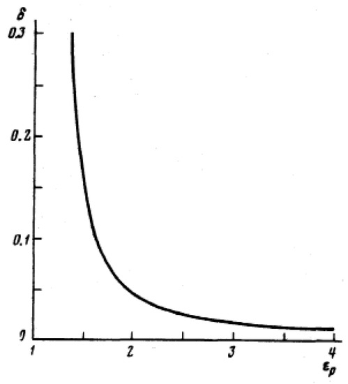
Figure 5. Correction on non-adiabaticity of the motion of nuclei, $\delta$, cf. [7], for collisions U+U as a function of the positron energy ${ϵ}_p$.

Numerical calculations [18,48] have shown that $R_{\mathrm{cr}}$ rapidly increases with increasing charge $Z=Z_1+Z_2$ of colliding nuclei. The cross section of the spontaneous production of positrons increases in this case $\propto R_{\mathrm{cr}}^{7/2}$, while the correction for the non-adiabaticity of the tunneling decreases as $1/R_{\mathrm{cr}}$ at a fixed ${ϵ}_p$. Therefore, it would be more convenient to perform experiments with heavier nuclei, for which $R_{\mathrm{cr}}$ is larger.

7. Many-Particle Semiclassical Approximation. Electron Condensation in Upper Continuum

7.1. Screening of a Source of Positive Charge in Presence of External Electrons

In a many-particle problem, most of the electrons in spherically symmetric potential well, $V<0$, have angular momenta $l\gg 1$. Thereby, to find distribution of the charge, we may deal with a more simple Klein–Gordon–Fock Equation (1) while assuming $j\simeq l$. The value of the maximum momentum, at which the electron placed in the positively charged ion where all levels with energies less than ${ϵ}_{\mathrm{bound}}$ are already occupied is bound, satisfies the condition

$$p_{max}=\sqrt{{({ϵ}_{\mathrm{bound}}-V)}^2-m^2}$$

(161)

with ${ϵ}_{\mathrm{bound}}\ge -m$. If there is a sufficient amount of external electrons, the resulting system is charge-neutral. In this case, we should put ${ϵ}_{\mathrm{bound}}=m$. Subsequently, $p_{max}=\sqrt{-2mV+V^2},$ and taking into account that each cell of the phase space can only be occupied by two electrons of opposite spin, we have

$$n_e=\frac{p_{max}^3}{3{\pi }^2}=\frac{{(-2mV+V^2)}^{3/2}}{3{\pi }^2}.$$

(162)

Thus, the relativistic Thomas–Fermi equation renders

$$\Delta V=4\pi e^2\left[n_{\mathrm{nucl}}-\frac{{(-2mV+V^2)}^{3/2}}{3{\pi }^2}\right],$$

(163)

$n_{\mathrm{nucl}}$ is the charged density of the nucleus. It is curious to note that such an equation for neutral atom has been introduced long ago [98], but a relativistic term was then treated as a small correction in nonrelativistic limit $|V|\ll m$.

7.2. Filling of the Vacuum Shell by Electrons

Note that, even in the absence of external electrons, which may fill the empty states, in case when the potential well $V<-2m{c}^2$ electrons and positrons can be created already from the vacuum in the absence of any external electrons. Positrons go off to infinity, whereas electrons screen the initial positive charge of the source. In this case, we should put ${ϵ}_{\mathrm{bound}}=-m$. Subsequently, the relativistic Thomas–Fermi equation renders, cf. [1,2,99],

$$\Delta V=4\pi e^2\left[n_{\mathrm{nucl}}-\frac{{(2mV+V^2)}^{3/2}}{3{\pi }^2}\theta (2mV+V^2)\right],$$

(164)

where $\theta \left(x\right)$ is the step-function, with the boundary conditions on the boarder of the ion

$$V\left(r_i\right)=-2m=-Z_i{e}^2/r_i,V^{\prime }\left(r_i\right)=Z_i{e}^2/r_i^2,$$

(165)

and with $V\left(r\right)=-Z_i{e}^2/r$ for $r>r_i$. Reference [99] presented numerical solutions. The thorough analytical and numerical study of the problem of the filling of the vacuum shell by many electrons was performed in an independent study [1,2]. This phenomenon was called “electron condensation”, demonstrating that all of the vacuum levels are filled by electrons of the lower continuum, cf. [42].

7.3. A Detailed Derivation of Relativistic Thomas-Fermi Equation

The electron density can be found by direct summation of the moduli squared of the wave functions [2]:

$$n_e=-\sum _{n\kappa m}{|{\psi }_{n\kappa m}|}^2,$$

(166)

where ${\psi }_{n\kappa m}$ are semiclassical wave functions presented in Equations (95)–(100). Actually, we need wave functions in the classically allowed region given by (95).

Differentiating quantization rule (108) over n, we obtain

$$\frac{\partial ϵ}{\partial n}{\int }_{r_0}^{r_{-}}\frac{ϵ-V}{p}dr\simeq \pi ,$$

(167)

where we dropped the term $\frac{\partial }{\partial n}\frac{\kappa w}{pr}$, which only leads to a small correction $|w|/V^2\sim 1/{\zeta }^2$, cf. [5].

From (167) and (96), we obtain

$$C_1={\left(\frac{1}{\pi }\frac{\partial ϵ}{\partial n}\right)}^{1/2}.$$

(168)

Using that ${\sum }_{m=-j}^j{|Y_{lm}|}^2=(2j+1)/\left(4\pi \right)$, where $Y_{lm}$ is the spherical function, from Equation (166), we have

$$n_e\left(r\right)=-\sum _{n\kappa }\frac{2j+1}{4{\pi }^2}\frac{\partial ϵ}{\partial n}\frac{ϵ-V}{p{r}^2}.$$

(169)

Here, we replaced ${sin}^2{\theta }_1$ and ${sin}^2{\theta }_2$ by $1/2$ due to multiple oscillations. Replacing summation in n by integration, we find

$$n_e=-\frac{1}{4{\pi }^2}\sum _j{N}_j=-\frac{1}{4{\pi }^2}\sum _j\frac{2(j+1/2)}{r^2}\sqrt{{({ϵ}_{\mathrm{bound}}-V)}^2-m^2-{(j+1/2)}^2/r^2}.$$

(170)

Doing further integration in j with ${ϵ}_{\mathrm{bound}}=-m$, we recover (164).

Now, let us estimate the number of electrons in the vacuum shell, for which single-particle approximation fails, i.e., number of levels, for which the width has no exponential smallness. Integrating (170) over the volume, we find the number of levels with momenta $j\le \kappa -1/2$,

$$\delta \left(\kappa \right)=\frac{1}{N_e}\sum _{j=1/2}^{\kappa -1/2}{N}_j=c{\kappa }^2,$$

(171)

where

$$c=3I_1/\left(2I_2\right),I_1=\int {(V^2+2mV)}^{1/2}dr,I_2=\int {(V^2+2mV)}^{3/2}{r}^{2}dr,$$

(172)

$V^2\ge -2mV$. In particular, for $V=-\zeta /r$ with logarithmic accuracy, we obtain

$$I_1=\zeta ln(\zeta /R_{\mathrm{nucl}}),I_2={\zeta }^{3}ln(\zeta /R_{\mathrm{nucl}}),c=3/\left(2{\zeta }^2\right).$$

(173)

For $\zeta \gg 1$ and ${\kappa }_0={(\zeta /\pi )}^{1/2}$ it follows that

$$\delta \left({\kappa }_0\right)=3/\left(2\pi \zeta \right)\ll 1.$$

(174)

Getting (171), we counted all states with $|\kappa |<{\kappa }_0$, whereas not all of them have exponentially suppressed $\mathsf{\Gamma }$. Taking a correction (174) into account leads to the appearance of a numerical factor $ln({\kappa }_0/R_{\mathrm{nucl}})/ln(\zeta /R_{\mathrm{nucl}})\simeq 1/4$ for $\zeta \gg 1$ since $R\propto {\zeta }^{1/3}$. We estimate $\delta \simeq 0.1/\zeta$, i.e., $\delta \sim 1\%$ for $Z\sim 1/e^3$. The smallness of $\delta$ characterizes the accuracy of Equation (164).

Taking the exchange and correlation corrections in the relativistic Thomas–Fermi equation into account is conveniently done by means of a variational method analogously to that is performed for the nonrelativistic Thomas–Fermi equation [100]. We arrive at

$$n_e\simeq -\frac{1}{3{\pi }^2}{[{(V^2+2mV)}^{1/2}-\nu (V+m)]}^3\theta (V^2+2mV),$$

(175)

$\nu \simeq e^2/\pi$. For $Z{e}^3\ll 1$ this correction can be safely dropped. For $Z{e}^3\gg 1$ it can be taken into account in Equation (164) by introducing the renormalized coupling constant $e^2\to e^2(1+3e^2/\pi )$, cf. [2].

Additionally, a correction appears due to that the dielectric permittivity of the vacuum, $\epsilon \left(eE\right)$, differs from unity, $e\overrightarrow{E}=-\nabla V$. Thus, one should replace $\Delta V\to \nabla \left(\epsilon \right(E)\nabla V)$ in Equation (164). However, this correction, as the correlation correction, is tiny, since $\epsilon \left(eE\right)=1-(e^2/\left(3\pi \right))ln(eE/m^2)$, and at distances $r\gtrsim 1/\left(a_Z\right)$ of our interest $\epsilon \left(eE\right)\simeq 1+O(e^2/\left(3\pi \right))$, cf. [49] and Equation (252), below.

7.4. Weak Screening, $1/e^2\ll Z\ll 1/e^3$

Consider the screening of the positively charged nucleus of the initial proton number Z and the radius R (typically $R_{\mathrm{nucl}}\simeq A^{1/3}/m_{\pi }$, $A\sim 2Z$). Assume that, inside the nucleus, the proton charge density is $n_p^0=const$. Introducing $\psi =-V/m-1$ in the region $V<-m$ ($\psi \ge 1$), where the electrons of the vacuum shell give some contribution to the screening of the charge Z, from Equation (164) we obtain

$$\Delta \left(m\psi \right)=\frac{4e^2{m}^3}{3\pi }{({\psi }^2-1)}^{3/2}\theta (\psi -1)-4\pi n_p^0\theta (R_{\mathrm{nucl}}-r),$$

(176)

$\theta \left(x\right)$ is the step-function. For $r>R_{\mathrm{nucl}}$, with the help of the replacement $x=r/r_i$, we obtain

$${\psi }_x^{″}+\frac{2{\psi }_x^{\prime }}{x}=\mu {({\psi }^2-1)}^{3/2},\psi \left(1\right)=1,{\psi }^{\prime }\left(1\right)=-2,\mu =\frac{4e^2{m}^2{r}_i^2}{3\pi }=\frac{{\left(Z_{\mathrm{obs}}{e}^3\right)}^2}{3\pi }.$$

(177)

Here, $Z_{\mathrm{obs}}$ is the charge seen at infinity. Because $\mu \ll 1$, we may use expansion

$$\psi (x,\mu )={\psi }_0\left(x\right)+\mu {\psi }_1\left(x\right)+\dots$$

(178)

Subsequently, we have equations

$${\Delta }_x{\psi }_0=0,{\psi }_0\left(1\right)=1,{\psi }_0^{\prime }\left(1\right)=2,$$

(179)

$${\Delta }_x{\psi }_1=3{({\psi }_0^2-1)}^{3/2}{\psi }_0{\psi }_1,{\psi }_1\left(1\right)=0,{\psi }_1^{\prime }\left(1\right)=0.$$

(180)

At the edge of the nucleus $x=2mR/\zeta \ll 1$. At $x\ll 1$, we derive

$$1+\psi (x,\mu )=2x^{-1}[1+4\mu (-lnx+C_0)+O(x,{\mu }^2)],C_0=2ln2-11/3.$$

(181)

Inside the nucleus at the condition $Z{e}^3\ll 1$, the potential is close to the bare one. Setting $\psi =\zeta y\left(\mathsf{\Xi }\right)/\left(R_{\mathrm{nucl}}m\right)$, $\mathsf{\Xi }=r/R$, we obtain

$$y_{\mathsf{\Xi }}^{″}+\frac{2y_{\mathsf{\Xi }}^{\prime }}{\mathsf{\Xi }}=\frac{4e^2{R}^3}{3\pi \zeta }{\left(\frac{{\zeta }^2{y}^2}{R^2}-m^2\right)}^{3/2}-\frac{4\pi R^3{e}^2}{\zeta }{n}_p^0,r<R_{\mathrm{nucl}}.$$

(182)

Using that inside the nucleus $|V|\sim \zeta /R_{\mathrm{nucl}}\sim Z^{2/3}m\gg m$ and $\frac{4\pi }{3}{R}_{\mathrm{nucl}}^3{n}_p^0=Z$, we get

$$y_{\mathsf{\Xi }}^{″}+\frac{2y_{\mathsf{\Xi }}^{\prime }}{\mathsf{\Xi }}=-3+\nu y^3,\nu =\frac{4{\left(Z{e}^3\right)}^2}{3\pi }.$$

(183)

Because $\nu \ll 1$, we expand

$$y=y_0\left(\mathsf{\Xi }\right)+\nu y_1\left(\mathsf{\Xi }\right)+\dots$$

(184)

and get

$$y_0\left(\mathsf{\Xi }\right)=\frac{1}{2}(3-{\mathsf{\Xi }}^2),y_1\left(\mathsf{\Xi }\right)=C+{\mathsf{\Xi }}^{-1}{\int }_0^{\mathsf{\Xi }}{y}_0^3\left(x\right)x(\mathsf{\Xi }-x)dx.$$

(185)

Matching of V and $V^{\prime }$ at the edge of the nucleus yields

$$C=-1-{\int }_0^1{y}_0^3\left(x\right)xdx,$$

(186)

and

$$Z_{\mathrm{obs}}=Z\left[1-\frac{4}{3\pi }{\left(Z{e}^3\right)}^2(ln\frac{\zeta }{R}+C_1)+...\right],$$

(187)

$$C_1=ln2-\frac{8}{3}+{\int }_0^1{y}_0^3\left(x\right)x^{2}dx\simeq 1.38.$$

(188)

7.5. Strong Screening, $Z{e}^3\gg 1$

Continue to consider a nucleus with $Z\sim A/2$ and $R_{\mathrm{nucl}}\simeq Z^{1/3}/m_{\pi }$. Because R grows with Z, one may expect that, for a sufficiently large Z, most of the electrons enter the nucleus and the interior becomes charge-neutral, as infinite matter. For the bare nucleus, the energy that is associated with the electric field,

$${\mathcal{E}}_{\mathrm{el}}=\int \frac{{(\nabla V)}^2}{8\pi e^2}{d}^{3}x\sim Z^2{e}^2/R_{\mathrm{nucl}}\sim Z^{5/3}{e}^2{m}_{\pi },$$

(189)

increases with Z more sharply when compared to the binding energy $\sim A\sim Z$, thereby the volume-charged systems do not exist. The charge, if it exists, is repelled to the surface.

To approximately solve Equation (164), we now introduce variables $x=(r-R_{\mathrm{nucl}})/l$ and $V=-V_0\chi \left(x\right)$. Constant $V_0$ is found from the condition of the charge neutrality at $x\to -\infty$, i.e., $V_0^3/\left(3{\pi }^2\right)=n_p^0$ for $V_0\gg m$. Thus, in new variables, Equation (164) renders

$${\chi }_x^{″}{l}^{-2}+2{\chi }_x^{\prime }{l}^{-2}/(x+R_{\mathrm{nucl}}/l)=\frac{4\pi e^2{n}_p^0}{V_0}[{\chi }^3-\theta (-x)],$$

(190)

with boundary conditions $\chi (-\infty )=1$, $\chi (\infty )=0$. The latter condition just means that typical decrease of the potential occurs already at $x\sim l$ near the nucleus boundary, whereas the transition to the Coulomb law occurs at $x\gg l$. The solution at such large distances can only be found numerically.

Because, in dimensionless equation with dimensionless boundary conditions typical $|x|\sim 1$, for $R_{\mathrm{nucl}}\gg l$, which we assume, we can neglect the second term in l.h.s. of Equation (190). In this case, geometry becomes one-dimensional and Equation (190) reduces to

$${\chi }^{″}={\chi }^3-\theta (-x),$$

(191)

where we determined the length l, as

$$l^{-2}=4\pi e^2{n}_p^0/V_0=4e^2{(\pi /3)}^{1/3}{\left(n_p^0\right)}^{2/3}.$$

(192)

Taking the boundary conditions into account, the first integral of Equation (191) is as follows

$$2{\chi }^{\prime 2}={\chi }^4+(-4\chi +3)\theta (-x),$$

(193)

and the final solution is

$$\chi \left(x\right)=1-3{[1+2^{-1/2}\mathrm{sh}(a-x/\sqrt{3})]}^{-1}x<0,\mathrm{sh}a=11\sqrt{2},$$

(194)

$$\chi \left(x\right)=2^{1/2}{(x+b)}^{-1},x>0,b=4\sqrt{2}/3.$$

(195)

Note that Equation (191) allows for very simple approximate solution for $x<0$. To get it, we write $\chi =1+\psi$, $\psi \ll 1$ and, from (191), find

$$\chi \left(x\right)\simeq 1-C^{\prime }{e}^{x\sqrt{3}}.$$

(196)

Using the boundary conditions at $x=0$, we find $C^{\prime }\simeq 0.24.$ This solution with an error less than 1.5% coincides with the exact solution.

The maximal strength of the electric field is reached at the edge of the nucleus,

$$E_{\max }=\frac{9\pi \sqrt{2}}{16}{\left(\frac{3}{\pi }\right)}^{1/6}{\left(n_p^0\right)}^{2/3}\simeq 8.2·{10}^{19}\mathrm{V}/\mathrm{cm},$$

that $\simeq 6000$ times exceeds the electron QED unit $E_{\mathrm{QED}}=m^2{c}^3/\left(e\hslash \right)\simeq 1.3·{10}^{16}\mathrm{V}/\mathrm{cm}$. Note that, to obtain this conclusion, we essentially used the relation $R_{\mathrm{nucl}}\sim Z^{1/3}/m_{\pi }$.

The energy of the system can be recovered by the integration of Equation (164). For $|V|\gg m$, we have

$$\mathcal{E}=\int \left[-\frac{{(\nabla V)}^2}{8\pi e^2}-\frac{V^4}{12{\pi }^2}-n_p^0\theta (R_{\mathrm{nucl}}-r)V\right]d^{3}x.$$

(197)

Expression (189) is obtained, after one puts to zero the term $\frac{V^4}{12{\pi }^2}$ related to the electron condensation and employs the partial integration and Poisson equation.

In our case, $\nabla V=0$ inside the system for $R_{\mathrm{nucl}}\gg l$ and $V_0={\left(3{\pi }^2{n}_p^0\right)}^{1/3}$. With these values, Equation (197) yields

$$\mathcal{E}=\frac{V_0^4}{4{\pi }^2}·\frac{4\pi }{3}{R}_{\mathrm{nucl}}^3.$$

(198)

Accordingly, the energy is reduced to the kinetic energy of the degenerate relativistic electron gas filling all energy levels of the vacuum shell with $ϵ<-m$. One should add to it the energy that is associated with the strong interaction of nucleons resulting in the binding of the ordinary atomic nuclei. In such a way, we get transition to the description of infinite matter. We see that, not taking into account a pion condensate or some other complex processes, we have $\mathcal{E}>0$ and such a matter, without inclusion of the gravity, is unstable, cf. [2,43].

If, instead of the usage that $A\sim 2Z$, we assumed the validity of the $\beta$ equilibrium conditions, $n\leftrightarrow p+e+\overline{\nu }$, we would get $A\gg Z$, and taking into account the gravity and the filling of all electron levels up to $ϵ=m$, we would recover the description of the ordinary neutron-star matter, cf. [43].

7.6. Falling to the Center in Relativistic Thomas-Fermi Equation

For $V=-Z{e}^2/r$, the number of electrons filling the vacuum shell is

$$N_e\simeq {\int }^r\frac{{|V|}^3}{3{\pi }^2}{d}^{3}x\sim ln1/\left(rm\right)\to \infty$$

(199)

for $r\to 0$.

Now, consider a formal solution of Equation (164) at $r<r_i$ with boundary conditions (165) corresponding to that for $r>r_i$, we deal with the Coulomb law with the charge equal to the observable charge $Z_{\mathrm{obs}}$. As we shall see, such a problem has a unique solution independently on the charge $Z_0$ put in the center, i.e., at $r\to 0$. It proves to be that the exact solution of Equation (164) has the pole singularity already at a finite value $r=r_{\mathrm{pole}}\left(\mu \right)$. In a weak screening limit from Equation (176), for $r\to r_{\mathrm{pole}}\left(\mu \right)$, in the dimensionless variable $x=r/r_i$, $x_{\mathrm{pole}}=r_{\mathrm{pole}}/r_i$, we get [3],

$$\psi (x,\mu )=\frac{C}{x-x_{\mathrm{pole}}}\left[1+\frac{a_1(x-x_{\mathrm{pole}})}{x_{\mathrm{pole}}}+\frac{a_2{(x-x_{\mathrm{pole}})}^2}{x_{\mathrm{pole}}^2}+...\right],C={(\mu /2)}^{-1/2},$$

(200)

$a_1=-1/3$, $a_2=2/9+\mu x_{\mathrm{pole}}^2/6$, ...The substitution of (200) in Equation (176) allows for finding coefficients $a_n$, but does not allow for recovering dependence $x_{\mathrm{pole}}\left(\mu \right)$. To obtain a full solution of the problem, we need to solve Equation (176) with the boundary conditions (165) in the whole interval $1>x>x_{\mathrm{pole}}\left(\mu \right)$. The numerical solution yields

$$x_{\mathrm{pole}}\left(\mu \right)=r_{\mathrm{pole}}\left(\mu \right)/r_i=D\left(\mu \right)e^{-1/\left(8\mu \right)},\mu \to 0.$$

(201)

Pre-exponential factor $D\left(\mu \right)$ is shown in Figure 6. For $Z_{\mathrm{obs}}\gg 1/\left(2e^2\right)$ with increasing $Z_{\mathrm{obs}}$ the pole moves towards the value $1/m$.

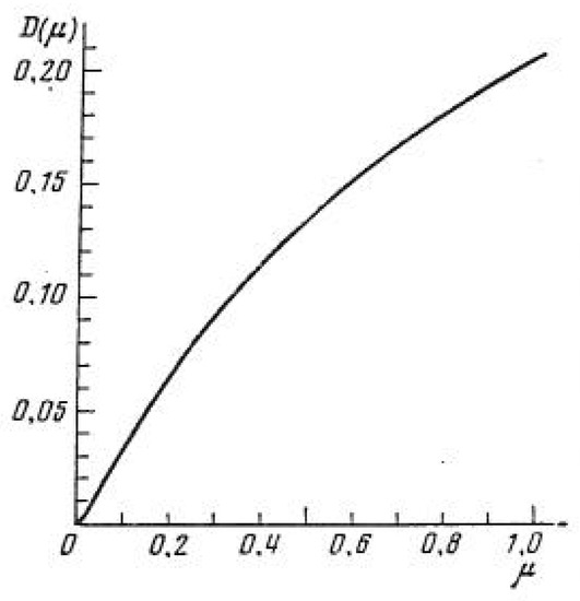
Figure 6. Pre-exponential factor $D(\mu )$ in Equation (201), cf. [3].

We conclude that, in the many-particle problem, including the electron condensation but not including the polarization of the vacuum, the falling to the center manifests itself in the presence of the pole at a distance $r_{\mathrm{pole}}\left(\mu \right)$. Accordingly, in the problem of the distribution of the charge at $r\ll 1/m$, there appeared a typical size $r_{\mathrm{pole}}\left(\mu \right)$, which characterizes the electron condensation, where all of the states are occupied according to the Pauli principle. Thus, we have found a relation between $Z_{\mathrm{obs}}$ and $Z\left(r_0\left(\mu \right)\right)$, for the size of the source $r_0>r_{\mathrm{pole}}\left(\mu \right)$. To match this exterior solution with the interior solution for $r<r_0$, we may use either model I or model II. It is important that $r_0$ should be larger than $r_{\mathrm{pole}}\left(\mu \right)$.

At this instance, we should remind about the existence of the Landau pole for $r=r_{\mathrm{L}}\simeq e^{-3\pi /\left(2e^2\right)}/m$, which appears within the multi-particle problem of the polarization of the electron-positron vacuum near the Coulomb center, cf. [49]. Comparison of the exponential factors shows that, for $Z_{\mathrm{obs}}<1/\left(2e^2\right)$, we have $r_{\mathrm{L}}>r_{\mathrm{pole}}\left(\mu \right)$ and, for $Z_{\mathrm{obs}}>1/\left(2e^2\right)$, we have $r_{\mathrm{L}}<r_{\mathrm{pole}}\left(\mu \right)$. Thus, in the case $Z_{\mathrm{obs}}<1/\left(2e^2\right)$, with decreasing r, first the polarization of the vacuum becomes effective and only at r in a narrow vicinity of $r_{\mathrm{L}}$, where $Z\left(r\right)>1/e^2$, the electron condensation becomes to be efficient. For $Z_{\mathrm{obs}}>1/e^2$, the electron condensation first becomes effective and only at r in a narrow vicinity of $r_{\mathrm{pole}}\left(\mu \right)>r_{\mathrm{L}}$ the polarization of the vacuum begins to contribute, see a detailed discussion below in Section 9.

Note that the value $Z_{\mathrm{obs}}{e}^2$ plays a role of an effective coupling in description of semimetals and effects under discussion might be relevant in this case, cf. [60].

It is curious to note that the inclusion of gravitational field of the source into consideration modifies the QED problem of the distribution of the charge while taking the electron condensation into account, cf. [101]. Solution (200) is modified at r approaching $r_{\mathrm{pole}}$. After a growth, solution continues up to $r\to 0$ as $V\to -Z_0{e}^2/r$ with $Z_0\sim Z_{\mathrm{obs}}^{2/3}/{\left(eG{m}^2\right)}^{1/3}$, where G is the gravitational constant. Additionally, the pole solution (200) disappears in case of the electron condensation in presence of a strong uniform magnetic field, cf. [102].

At the end, note [3] that Equation (164) can be solved within the main logarithmic approximation [49,103], being broadly used in different problems of the quantum field theory, see a discussion below in Section 8.1. Introducing variables $\psi =\varphi \left(x\right)/x$, $t=-lnx$, $x=r/r_i$, in ultra-relativistic limit $|V|\gg m$, we obtain

$${\varphi }_t^{″}+{\varphi }_t^{\prime }=\mu {\varphi }^3.$$

(202)

Assume $\varphi ={\sum }_{n=1}^{\infty }{\mu }^n{\varphi }_n$ with ${\varphi }_n=C_n{t}^n+O\left(t^{n-1}\right)$ for $t\to \infty$. Subsequently, we get solution $C_n=2^{n+1}\left(2n\right)!/{(n!)}^2$ that finally yields $\psi (x\to 0)=C_n{x}^{-1}{(-lnx)}^n+\dots$ A summation of these terms yields solution

$$\psi \left(x\right)=2x^{-1}{(1+8\mu lnx)}^{-1/2},$$

(203)

which has a spurious square-root singularity at $x\to x_0=e^{-1/\left(8\mu \right)}$, whereas the exact solution has the pole. Thus, this example demonstrates the possible deficiencies of the main logarithmic approximation in cases when we deal with divergent series.

8. Polarization of Vacuum

8.1. Polarization of Vacuum in Uniform Stationary Electric and Magnetic Fields

In the absence of external electromagnetic fields, electrons of the lower continuum have infinite energy

$${\mathcal{E}}_0=\sum _{\overrightarrow{p}\sigma }{ϵ}_{\overrightarrow{p}\sigma }^{0,-},$$

(204)

where ${ϵ}_{\overrightarrow{p}\sigma }^{0,-}=-\sqrt{m^2+{\overrightarrow{p}}^2}$ are negative-sign solutions of the dispersion relation of the free Dirac equation. In pure QED, i.e., at ignorance of gravitational effects, infinite constant (204) has no sense, being subtracted within renormalization procedure. In the presence of the electric and magnetic fields energy levels of the lower continuum, ${ϵ}_{\overrightarrow{p}\sigma }^{-}$ are changed. The difference

$$\mathcal{E}-{\mathcal{E}}_0=\sum _{\overrightarrow{p}\sigma }{ϵ}_{\overrightarrow{p}\sigma }^{-}-\sum _{\overrightarrow{p}\sigma }{ϵ}_{\overrightarrow{p}\sigma }^{0,-}$$

(205)

has the physical meaning.

Heisenberg and Euler considered the polarization of the electron-positron vacuum in the static uniform stationary electric and magnetic fields [104], cf. [49,105,106]. For the case of uniform purely magnetic field calculation is more transparent. Eigenvalues of the Dirac equation are

$${ϵ}_{\overrightarrow{p}\sigma }^{\pm }=\pm \sqrt{m^2+p_z^2+|e|H(2n+1)+|e|H\sigma }n=0,1,\dots ,\sigma =\pm 1.$$

(206)

The ground-state corresponds to the “−” sign solution. To calculate the sum (205), one uses that the number of states in the interval $d{p}_z$ in the uniform magnetic field is given by

$$\frac{|eH|}{{\left(2\pi \right)}^2}d{p}_z{V}_3,$$

(207)

cf. [39]. Taking into account the double degeneracy of levels with n, $\sigma =1$ and $n+1$, $\sigma =-1$ excluding ground state $n=0$, $\sigma =-1$, with ${ϵ}_{\overrightarrow{p}\sigma }^{-}$ solution, one obtains

$$\mathcal{E}=-{\int }_{-\infty }^{\infty }2\frac{|e|H}{{\left(2\pi \right)}^2}\sum _{n=1}^{\infty }\sqrt{m^2+p_z^2+2|e|Hn}d{p}_z{V}_3+\frac{|e|H}{{\left(2\pi \right)}^2}{\int }_{-\infty }^{\infty }\sqrt{m^2+p_z^2}d{p}_z{V}_3.$$

(208)

The divergence of integrals is removed by the subtraction of ${\mathcal{E}}_0$. To do this renormalization, it is convenient to calculate a convergent derivative of the energy

$$\frac{{\partial }^2\mathcal{E}}{\partial {\left(m^2\right)}^2}=\frac{|e|H}{8{\pi }^2}{\int }_0^{\infty }{e}^{-m^2\eta }\left[\frac{2}{1-e^{-2|e|H\eta }}-1\right]d\eta V_3=\frac{|e|H}{8{\pi }^2}{\int }_0^{\infty }{e}^{-m^2\eta }\mathrm{cth}(|e|H\eta )d\eta V_3.$$

(209)

After double integration and subtraction of the value ${\mathcal{E}}_0$, we obtain

$$\mathcal{E}-{\mathcal{E}}_0=\frac{V_3}{8{\pi }^2}{\int }_0^{\infty }\frac{e^{-m^2\eta }}{{\eta }^3}[\eta |e|H\mathrm{cth}(\eta |e|H)-1]d\eta +C_1+C_2{m}^2.$$

(210)

The contr-terms $C_1$ and $C_2$ do not depend on $m^2$, but may depend on H.

In the case of uniform stationary fields $\overrightarrow{E}$ and $\overrightarrow{H}$, the Lagrangian density $\mathcal{L}=-\mathcal{E}$ can only be a function of Lorentz invariants ${\overrightarrow{E}}^2-{\overrightarrow{H}}^2$ and $\overrightarrow{E}\overrightarrow{H}$. Note here that, in the presence of the sources of the current, the Lagrangian density additionally depends on $j^{\mu }{A}_{\mu }$.

In the case under consideration employing arguments of dimensionality and parity in $\overrightarrow{H}$, one can write

$$\mathcal{L}\left(H\right)={\mathcal{L}}_0\left(H\right)+{\mathcal{L}}^{\prime }\left(H\right)=-\frac{H^2}{8\pi }+m^{4}f(H^2/m^4).$$

(211)

The first term is the ordinary Lagrangian density in the magnetic field, whereas the second term is the contribution of the polarization of the vacuum in the magnetic field. In Equation (211), there are no terms odd in $m^2$, so $C_2=0$. Using that $\mathrm{cth}x=x^{-1}+x/3$ for $x\to 0$, we may see that the absence of $H^2$ term ${\mathcal{L}}^{\prime }\left(H\right)$ corresponds to the choice

$$C_1=-\frac{H^2{e}^2}{3·8{\pi }^2}{\int }_0^{\infty }{e}^{-\eta }\eta d\eta .$$

(212)

In the case of uniform static magnetic and electric fields, function $f\left(H\right)$ in (211) should be replaced by

$$f(H,E)=f(H^2-E^2,{(\overrightarrow{E}\overrightarrow{H})}^2).$$

(213)

At $H=0$, thereby $f(0,E)=f(-E^2,0)$. At $E=0$, $f(H,0)=f(H^2,0)$. From here, we see that $f(0,E)=f(H=iE,0)$, i.e., the expression (211) for the case $H\ne 0$, $E=0$, remains valid after replacement $H\to iE$. Note that $f(-E^2,0)$ has a small imaginary part associated with a possibility of the tunneling of a part of electrons, which initially occupied levels of the lower continuum, to the upper continuum. Created in a sufficient number, the electron-positron pairs change the spatial dependence of the electric field. In a realistic treatment of the problem one should consider electron and positron condensates occurred near the plates of the capacitor, which produced initially uniform electric field.

In case of strong uniform electric and magnetic fields $|eE|/m^2\gg 1$ and $|eH|/m^2\gg 1$, with a logarithmic accuracy from Equations (210), (212), one finds expressions for the dielectric and magnetic permittivities [49,104]:

$${\epsilon }_{\mathrm{HE}}\left(E\right)=1-\frac{e^2}{3\pi }ln(|eE|/m^2)+O\left(e^2\right),{\mu }_{\mathrm{HE}}\left(H\right)=1-\frac{e^2}{3\pi }ln(|eH|/m^2)+O\left(e^2\right).$$

(214)

The corresponding contributions to the energy of the lower continuum are

$${\mathcal{E}}_E=\int d^{3}x\frac{\epsilon (\nabla V){(\nabla V)}^2}{8\pi e^2},{\mathcal{E}}_H=\int d^{3}x\frac{\mu \left(H\right)H^2}{8\pi e^2}.$$

(215)

Note that expressions (214) are derived with the logarithmic accuracy, i.e., at the assumption that $ln(|eE|/m^2)|\gg 1$ and $ln(|eH|/m^2)|\gg 1$. Thereby, they are also formally applicable for negative values of $\epsilon$ and $\mu$ provided for the calculation of the vacuum energy in stationary uniform electric and magnetic fields one may employ the single-particle Dirac equation. At this assumption they are invalid only in a narrow region of fields, where $|\frac{e^2}{3\pi }ln(|eE|/m^2)|\sim O\left(e^2\right)$ and $|\frac{e^2}{3\pi }ln(|eH|/m^2)|\sim O\left(e^2\right)$. The result (214) also follows from the Dyson equation for the photon propagator that was calculated at one-loop, but with the electron Green functions that are dressed by the background field. In such an approximation, the radiative photon corrections to the electron Green function and vertices in the photon polarization operator are dropped. Figure 7 shows the effective action with one-particle irreducible (1PI) diagrams presented up to two-loops. The same result (214) is also recovered within the so-called main logarithmic resummation, when $e^{2l}{ln}^l\left(eE\right)$, $e^{2l}{ln}^l\left(eH\right)$ terms in the Dyson equation for the photon Green function are summed up, whereas terms $e^{2l}{ln}^{l-1}\left(eE\right)$, $e^{2l}{ln}^{l-1}\left(eH\right)$ are disregarded, cf. [49,103,106,107,108,109]. The radiative photon corrections to the electron Green function continue to be disregarded. The difference between two approximations is only manifested in the region where $e^4{ln}^2\left(eE\right)\gtrsim e^2$, $e^4{ln}^2\left(eH\right)\gtrsim e^2$. At the two-loop order, the term that is included in the effective action is given by the sandwich diagram (the one-particle-irreducible (1PI) contribution). The resulting dielectric and magnetic permittivities up to correction terms are

$$\begin{array}{c}\hfill {\epsilon }_{1\mathrm{PI}}\left(E\right)\simeq {\epsilon }_{\mathrm{HE}}\left(E\right),{\mu }_{1\mathrm{PI}}\left(H\right)\simeq {\mu }_{\mathrm{HE}}\left(H\right).\end{array}$$

(216)

Figure 7. The 1PI effective action shown up to two-loops. Double solid line shows the electron Green function dressed by the background field. Wavy line shows photon Green function.

Recently, Refs. [110,111,112] studied the role of the one-particle reducible (1PR) loop diagrams. In this scheme, Figure 8 shows the effective action up to four loops. These 1PR diagrams yield zero contribution in the case of constant fields [107], since, in the case of purely constant classical fields, the four-current term is absent. However, the argument for the vanishing of the current no longer holds as soon as the external field supports a slightest inhomogeneity somewhere in the space-time [110].

Figure 8. The 1PR effective action shown up to four loops summed up in [112]. Double solid line shows electron Green function dressed by the background field. The wavy line shows photon Green function.

In the latter case, all possible 1PR loop diagrams, being included, can be constructed from the 1PI one-loop constant-field diagram. The result of such a resummation of the diagrams in the strong-field limit yields [112],

$$\begin{array}{cc}& {\epsilon }_{1\mathrm{PR}}\left(E\right)=1-\frac{e^2}{3\pi }ln\frac{|eE|}{m^2}\left(1+\frac{1}{2}\frac{e^{2}ln(|eE|/m^2)}{3\pi (1-(e^2/\left(3\pi \right))ln(|eE|/m^2)}\right)\left[1+O(1/ln\frac{|eE|}{m^2})\right],\\ & {\mu }_{1\mathrm{PR}}\left(H\right)=1-\frac{e^2}{3\pi }ln\frac{|eH|}{m^2}\left(1+\frac{1}{2}\frac{e^{2}ln(|eH|/m^2)}{3\pi (1-(e^2/\left(3\pi \right))ln(|eH|/m^2)}\right)\left[1+O(1/ln\frac{|eH|}{m^2})\right].\end{array}$$

(217)

Note that, although, formally, these expressions are derived in the approximation $ln(|eE|/m^2),ln(|eH|/m^2)\gg 1$, as noticed in [112], they cannot be valid at least in the region where $|1-(e^2/\left(3\pi \right))ln(|eE|/m^2)|,|1-(e^2/\left(3\pi \right))ln(|eH|/m^2)|\lesssim e^2$, due to the presence of the pole in expressions (217). For example, the dielectric permittivity ${\epsilon }_{1\mathrm{PR}}\left(E\right)\to -\infty$ for $(e^2/3\pi )ln(|eE|/m^2)\to 1-\delta$ and ${\epsilon }_{1\mathrm{PR}}\left(E\right)\to +\infty$ for $(e^2/3\pi )ln(|eE|/m^2)\to 1+\delta$ for $\delta \to 0$. Conversely, (214) and (216) do not produce any non-physical singularities, yielding zero, rather than the pole at $(e^2/3\pi )ln(|eE|/m^2)\to 1$. In the region where $ln(|eE|/m^2),ln(|eH|/m^2)\gg 3\pi /e^2$ expressions (214), (217) yield

$$\begin{array}{cc}& {\epsilon }_{\mathrm{HE}}\left(E\right)\to -\frac{e^2}{3\pi }ln(|eE|/m^2),{\mu }_{\mathrm{HE}}\left(H\right)\to -\frac{e^2}{3\pi }ln(|eH|/m^2),\\ & {\epsilon }_{1\mathrm{PR}}\left(E\right)\to -\frac{1}{2}\frac{e^2}{3\pi }ln(|eE|/m^2),{\mu }_{1\mathrm{PR}}\left(H\right)\to -\frac{1}{2}\frac{e^2}{3\pi }ln(|eH|/m^2).\end{array}$$

(218)

In the one-loop order, results (214)–(217) coincide. Beyond the one-loop approximation, various partial resummation schemes produce different results.

To proceed further, we will use expression

$$\begin{array}{c}\hfill \epsilon \left(E\right)=1-\nu \frac{e^2}{3\pi }ln(|eE|/m^2).\end{array}$$

(219)

With $\nu =1$, we deal with the result [49,104,106], for $\frac{e^2}{3\pi }ln(|eE|/m^2)<1$ being recovered within the main logarithmic approximation for the 1PI diagrams and, for $\frac{e^2}{3\pi }ln(|eE|/m^2)\ll 1$, being also recovered within the main logarithmic approximation applied for the 1PR diagrams. With $\nu$, being a very smooth function of the tortoise variable $ln(|eE|/m^2)$ varying from 1 at $|eE|\sim m^2$ to $1/2$ for $ln(|eE|/m^2)\gg 3\pi /e^2$, we recover the asymptotic behavior that was derived in [112] with the included 1PR loop diagrams.

At the end, we stress that both main-logarithmic resummation schemes considered above may be not valid for $(e^2/3\pi )ln(|eE|/m^2),(e^2/3\pi )ln(|eH|/m^2)\to \infty$, since the dropped sub-series of the diagrams may yield divergent contributions. We have demonstrated examples of such a kind in Section 7.6, cf. [3]. A summation of the 1PR diagrams leads to the appearance of the pole in expressions ${\epsilon }_{1\mathrm{PR}}\left(E\right)$ and ${\mu }_{1\mathrm{PR}}\left(H\right)$ for $(e^2/3\pi )ln(|eE|/m^2)=1,(e^2/3\pi )ln(|eH|/m^2)=1$. Moreover, recall that the expansion in the number of loops is a semiclassical series. The latter series is an asymptotic one, and retaining too many terms may worsen the convergence of the series to the exact solution. Bearing this in mind, the result that is given by ${\epsilon }_{\mathrm{HE}}\left(E\right),{\mu }_{\mathrm{HE}}\left(H\right)$ looks more physically motivated. Nevertheless, further on, we use Equation (219) varying parameter $\nu$ in the interval $(1/2,1)$ to recover both asymptotics in Equation (218).

8.2. Noninteracting Photon, Electron, and Spin-Zero Boson Propagators

The Green function of the free photon is given by

$$\begin{array}{c}\hfill i{D}_{\mu \nu }^0(x-x^{\prime })=<0|\widehat{T}{\widehat{A}}_{\mu }^{\mathrm{int}}\left(x\right){\widehat{A}}_{\nu }^{\mathrm{int}}\left(x^{\prime }\right)|0>,\end{array}$$

(220)

$\widehat{T}$ is the ordinary time ordering, operators are in interaction picture, cf. [49]. The most general form is as follows,

$$D_{\mu \nu }^0(x-x^{\prime })=g_{\mu \nu }{D}^0({(x-x^{\prime })}^2)-{\partial }_{\mu }{\partial }_{\nu }{D}_{\left(l\right)}^0({(x-x^{\prime })}^2),$$

(221)

$g_{\mu \nu }$ is the metric tensor. One usually uses the Feynmann gauge condition $D_{\left(l\right)}^0=0$.

For $D_{xx}^0=-D^0$, we have

$$D^0\left(k^2\right)=\frac{4\pi }{(k^2+i0)}.$$

(222)

In the Feynmann gauge,

$$D_{\mu \nu }^0\left(k^2\right)=g_{\mu \nu }\frac{4\pi }{(k^2+i0)}.$$

(223)

The free propagator of spin $1/2$ electron is

$$G_{ik}^0=-i<0|\widehat{T}{\widehat{\mathsf{\Psi }}}_i^0\left(x\right){\widehat{\overline{\mathsf{\Psi }}}}_k^0\left(x^{\prime }\right)|0>,$$

(224)

where $\overline{\mathsf{\Psi }}={\mathsf{\Psi }}^{†}{\gamma }_0$ and ${\mathsf{\Psi }}_i^0\left(x\right)$ satisfy the Dirac equation $({\gamma }^{\mu }{\widehat{p}}_{\mu }-m){\mathsf{\Psi }}_i^0\left(x\right)=0$.

Thus, the Fourier transform is

$$G^0\left(p\right)=\frac{1}{{\gamma }^{\mu }{p}_{\mu }-m},G^0\left(p\right)=\frac{{\gamma }^{\mu }{p}_{\mu }+m}{p^2-m^2}.$$

(225)

We may turn the contour in $p_0$ plane against clock arrow not touching poles and, then, we perform replacements $i{p}_0=p_4$, $i{x}_0=x_4$, $px=-\tilde{p}\tilde{x}=-(p_4{x}_4+\overrightarrow{p}\overrightarrow{x})$, $\tilde{p}=(\overrightarrow{p},p_4)$, $\tilde{x}=(\overrightarrow{x},x_4)$, $\int d{p}_0/i\to \int d{p}_4$. Let us present

$$\frac{1}{{\tilde{p}}^2+m^2}={\int }_0^{\infty }{e}^{-\alpha ({\tilde{p}}^2+m^2)}d\alpha ,$$

(226)

$$\begin{array}{cc}& G_{\mathrm{b}}^{0,\mathrm{ch}}\left(x\right)=\int \frac{d^{4}p}{{\left(2\pi \right)}^4}\frac{e^{-ipx}}{p_0^2-{\overrightarrow{p}}^2-m^2+i\delta }=-i{\int }_{-\infty }^{\infty }\frac{d^4\tilde{p}}{{\left(2\pi \right)}^4}\frac{e^{i\tilde{p}\tilde{x}}}{{\tilde{p}}^2+m^2}\\ & =-i{\prod }_{i=1}^4{\int }_{-\infty }^{\infty }\frac{d\tilde{p}}{2\pi }{e}^{i{\tilde{p}}_i{\tilde{x}}_i}{\int }_0^{\infty }d\alpha e^{-\alpha ({\tilde{p}}_i^2+m^2)}=-\frac{i}{16{\pi }^2}{\int }_0^{\infty }du{e}^{-m^2/u-{\tilde{x}}^{2}u/4},\end{array}$$

(227)

$u=1/\alpha$. For $\tilde{x}m\ll 1$, we may put $m=0$ and find

$$G_{\mathrm{b}}^{0,\mathrm{ch}}\left(x\right)=\frac{i}{4{\pi }^2{x}^2},\tilde{x}m\ll 1.$$

(228)

For $\tilde{x}m\gg 1$, we may use the pass method and present

$$-\frac{m^2}{u}-\frac{{\tilde{x}}^{2}u}{4}\simeq -m\tilde{x}-\frac{{\tilde{x}}^3{(u-u_m)}^2}{8m}$$

and we find

$$G_{\mathrm{b}}^{0,\mathrm{ch}}\left(x\right)=-i\sqrt{\frac{m}{32{\pi }^3{\tilde{x}}^3}}{e}^{-m\tilde{x}},\tilde{x}m\gg 1.$$

(229)

For Dirac electrons

$$G^0\left(x\right)=\int \frac{d^{4}p}{{\left(2\pi \right)}^4}{e}^{-ipx}\frac{{\gamma }^{\mu }{p}_{\mu }+m}{p^2-m^2}=(m+i{\gamma }^{\mu }{\partial }_{\mu })G_{\mathrm{b}}^{0,\mathrm{ch}}\left(x\right).$$

(230)

Thus, for $\tilde{x}m\ll 1$, we obtain $G^0\left(x\right)=\frac{{\gamma }^{\mu }{x}_{\mu }}{2{\pi }^2{x}^4}$, the electron Green function is odd function of its coordinate argument. The power law increase of $G^0$ for $r\to 0$ reflects the fact that there is no scale of the length, which could describe the free particle at $r\ll 1/m$. For $r\gg 1/m$, processes of polarization of the vacuum in the absence of external fields are suppressed as follows from Equation (229).

8.3. Dyson Equation for Photon Propagator

Taking the vacuum polarization diagrams in the first order perturbation theory in $e^2$ into account, the Dyson equation gets the form

$$\begin{array}{cc}& i{D}_{\mu \nu }(X_2-X_1)=i{D}_{\mu \nu }^0(X_2-X_1)\\ & +\int d^4{X}_3{d}^4{X}_{4}i{D}_{\mu \lambda }^0(X_2-X_3)\mathrm{Tr}\left[(-ie{\gamma }^{\lambda })i{G}^0(X_4-X_3)(-ie{\gamma }^{\rho })i{G}^0(X_3-X_4)\right]i{D}_{\rho \nu }^0(X_4-X_1).\end{array}$$

(231)

In the momentum representation, we obtain

$$i{D}_{\mu \nu }\left(k\right)=i{D}_{\mu \nu }^0\left(k\right)+i{D}_{\mu \lambda }^0\left(k\right)\int \frac{d^{4}p}{{\left(2\pi \right)}^4}\mathrm{Tr}\left[(-ie{\gamma }^{\lambda })i{G}^0(p+k)(-ie{\gamma }^{\rho })i{G}^0\left(p\right)\right]i{D}_{\rho \nu }^0\left(k\right)(-1).$$

(232)

The last factor $(-1)$ comes from the closed fermion loop. The next terms in the full Dyson equation are constructed analogously.

The sum of all irreducible diagrams (which cannot be separated by a single photon line) is called the photon polarization operator, $-i{\mathsf{\Pi }}_{\mu \nu }$. Thereby, in the lowest order $-i{\mathsf{\Pi }}_0^{\lambda \rho }=\mathrm{Tr}\left[(-ie{\gamma }^{\lambda })i{G}^0(p+k)(-ie{\gamma }^{\rho })i{G}^0\left(p\right)\right]$. In brief, notations Dyson equation renders

$$D=D^0+D^0\mathsf{\Pi }D.$$

(233)

In the lowest order in $e^2$ one has $\mathsf{\Pi }={\mathsf{\Pi }}_0$.

8.4. Calculation of Photon Polarization Operator

8.4.1. Case of a Weak Static Electric Field. Renormalization of Charge

To remove divergencies in observables, one employs renormalization procedure. Below, we demonstrate this procedure on an example of renormalization of the charge. One assumes that, initially, the action enters the bare coupling $e_0^2$ rather than physical one, $e^2=1/137$. As we shall see, the polarization characteristics are divergent for $r\to 0$. At the same time, the $r\to 0$ limit is legitimate, because QED is the theory with the local interaction. To proceed, one introduces the cut-value $r_0$, with performing the limit $r_0\to 0$ in final expressions. According to diagrammatic rules in the first non-vanishing order

$$-i{\mathsf{\Pi }}_0^{\mu \nu }=\mathrm{Tr}(-i{e}_0{\gamma }^{\mu })i{G}^0\left(x\right)(-i{e}_0{\gamma }^{\nu })i{G}^0(-x).$$

(234)

At $r>1/m$, in the case of weak external fields, the effects of polarization of vacuum should be suppressed, since the electron Green function and, thereby, the photon polarization operator decrease exponentially in Euclidean variables, cf. Equation (229). Therefore, consider the opposite limit case $\tilde{x}\ll 1/m$ when the effects of the polarization of the vacuum can be significant. We recognize that at short distances there is no scale of length, except the Compton wave length. Thus, $G^0$ and ${\mathsf{\Pi }}_{\mu \nu }^0$ should be power-law functions of $\tilde{x}$. We have

$$-i{\mathsf{\Pi }}_{\mu \nu }^0\left(x\right)=-e_0^2\mathrm{Tr}[\frac{{\gamma }_{\mu }\widehat{x}{\gamma }_{\nu }\widehat{x}}{4{\pi }^4{x}^8}]=-e_0^2\frac{2x_{\mu }{x}_{\nu }-x^2{\delta }_{\mu \nu }}{{\pi }^4{x}^8},$$

(235)

$$-i{\mathsf{\Pi }}_{00}^0(t,\overrightarrow{R})=-e_0^2\frac{t^2+{\overrightarrow{R}}^2}{{\pi }^4{(t^2-{\overrightarrow{R}}^2)}^4}.$$

(236)

In mixed $\omega ,\overrightarrow{R}$ representation:

$${\mathsf{\Pi }}_{00}^0(\omega =0,\overrightarrow{R})=\int d\tau {\mathsf{\Pi }}_{00}^0\left(R\right)=\frac{e_0^2}{4{\pi }^3{({\overrightarrow{R}}^2)}^{5/2}}.$$

(237)

Using Equation (221) with $D_{\left(l\right)}=0$, we have

$$A^0\left(x\right)=\int d^4{x}^{\prime }D(x,x^{\prime })j_{\mathrm{ext}}^0\left(x^{\prime }\right).$$

(238)

Multiplying Equation (233) by $e_0^2{n}_{\mathrm{ext}}(\overrightarrow{r})$ and integrating, we arrive at the Poisson equation for the static field $V(\overrightarrow{r})=e_0{A}_0^{\mathrm{n}.\mathrm{ren}}=e{A}_0^{\mathrm{ren}}$, being expressed in terms of non-renormalized quantities,

$$\Delta V\left(\overrightarrow{r}\right)=4\pi e_0^2(-n_{\mathrm{ext}}\left(\overrightarrow{r}\right)+4\pi \int K_{00}^0(\omega =0,\overrightarrow{R})d^{3}RV(\overrightarrow{r}+\overrightarrow{R})),$$

(239)

where in case of weak fields we took the polarization operator in the lowest order, i.e., $K_{00}^0(\omega =0,\overrightarrow{R})={\mathsf{\Pi }}_{00}^0(\omega =0,\overrightarrow{R})/e_0^2$. $K_{00}^0(\omega =0,\overrightarrow{R})$ does not depend on $e_0^2$. As will be shown below, $K_{00}^0(\omega =0,\overrightarrow{R})$ diverges for $r_0\to 0$.

Now, our aim is to rewrite the Poisson Equation (239) in the form

$$\Delta V=-4\pi e^2{n}_{\mathrm{ext}}(\overrightarrow{r}).$$

To perform this procedure of renormalization of the charge, we continue to consider the polarization of the vacuum in a weak field, i.e assuming $n_{\mathrm{ext}}$ to be small. Subsequently, we may use expansion

$$V(\overrightarrow{r}+\overrightarrow{R})\simeq V(\overrightarrow{r})+\nabla V(\overrightarrow{r})\overrightarrow{R}+\frac{1}{2}\frac{{\partial }^{2}V}{\partial R_i{\partial }_k{R}_k}{R}_i{R}_k+...$$

(240)

We may drop convergent terms in the expansion (240) irrelevant for the renormalization procedure. The term $\int K_{00}^0(\omega =0,\overrightarrow{R})d^{3}RV(\overrightarrow{r})$ should be put zero, since constant potential cannot produce polarization charges due to gauge invariance. The term $\int K_{00}^0(\omega =0,\overrightarrow{R})\overrightarrow{R}{d}^{3}R\nabla V(\overrightarrow{r})=0$ due to isotropy of the vacuum in the weak field. Hence, we obtain

$$\Delta V=-e_{\mathrm{ren}}^{2}4\pi n_{\mathrm{ext}},e_{\mathrm{ren}}^2=e^2=\frac{e_0^2}{1+\frac{4\pi }{6}{e}_0^2\int K_{00}^0(\omega =0,{\overrightarrow{R}}^2){\overrightarrow{R}}^2{d}^3\overrightarrow{R}}.$$

(241)

Finally, we derived a formal relation between the bare coupling constant $e_0^2$ and the physical one $e^2=1/137$. After this procedure is performed, we may say that all physical values already depend only on $e^2$. Thus, in the lowest approximation over $e_0^2$ using Equation (237) and relation between ${\mathsf{\Pi }}_{00}^0$ and $K_{00}^0$, we obtain

$$e^2=\frac{e_0^2}{1+\frac{e_0^2}{3\pi }ln\frac{1}{m^2{r}_0^2}},e_0^2=\frac{e^2}{1-\frac{e^2}{3\pi }ln\frac{1}{m^2{r}_0^2}},r_0\to 0,$$

(242)

The formal solution of the first equation for any $e_0^2>0$ yields $e^2\to 0$, rather than $e^2$. This is known as “the problem of the zero charge”, (or “Moscow zero”), cf. [49]. Strictly speaking, such a consideration suffers from inconsistency, since the inverse relation given by the second equation has so called Landau pole for

$$r=r_{\mathrm{L}}=\frac{1}{m}{e}^{-3\pi /\left(2e^2\right)}.$$

(243)

From the second Equation (242), for $r_0\to 0$, follows the solution

$$e_0^2\to -\frac{3\pi }{ln((1/\left(m^2{r}_0^2\right))}\left(1+\frac{3\pi }{e^{2}ln(1/\left(m^2{r}_0^2\right))}\right),$$

(244)

corresponding to $e_0^2<0$ and imaginary $e_0$. A similar procedure could be performed in four-invariant form for the 4-potential $e_0{A}^{\mu }$, instead of $e_0{A}_0$.

8.4.2. Case of a Strong Static Electric field

In the presence of a strong static electric field the electron polarization operator, even being considered with the only one-loop diagram, should be calculated with full electron Green functions, G, instead of free ones [42,53]. In this approximation, expression (234) is replaced by

$$-i{\mathsf{\Pi }}^{\mu \nu }=\mathrm{Tr}(-i{e}_0{\gamma }^{\mu })iG\left(x\right)(-i{e}_0{\gamma }^{\nu })iG(-x).$$

(245)

At this level, the Ward–Takahashi identity is only satisfied approximately. It can be fulfilled exactly after taking the higher order diagrams into account.

Multiplying Equation (233) by $e_0^2{n}_{\mathrm{ext}}(\overrightarrow{r})$, we derive the Poisson equation for the static field $V(\overrightarrow{r})=e_0{A}_0^{\mathrm{n}.\mathrm{ren}}=e{A}_0^{\mathrm{ren}}$, expressed in terms of non-renormalized quantities,

$$\Delta V(\overrightarrow{r})=-4\pi e_0^2(n_{\mathrm{ext}}(\overrightarrow{r})-4\pi \int K_{00}(\omega =0,\overrightarrow{r},\overrightarrow{R})d^{3}RV(\overrightarrow{r}+\overrightarrow{R})),$$

(246)

where $K_{00}(\omega =0,\overrightarrow{r},\overrightarrow{R},e_0^2)={\mathsf{\Pi }}_{00}(\omega =0,\overrightarrow{r},\overrightarrow{R},e_0^2)/e_0^2$. Being expressed in non-renormalized terms, both of these quantities depend on $e_0^2$. For $G\to G^0$, they transform to $K_{00}^0(\omega =0,\overrightarrow{r},\overrightarrow{R})={\mathsf{\Pi }}_{00}^0(\omega =0,\overrightarrow{r},\overrightarrow{R},e_0^2)/e_0^2$.

We again use expansion (240). The term $\int K_{00}(\omega =0,\overrightarrow{r},\overrightarrow{R})d^{3}RV(\overrightarrow{r})$ should be put to zero, since the constant potential cannot produce polarization charges due to the gauge invariance. The term $\int K_{00}(\omega =0,\overrightarrow{r},\overrightarrow{R})\overrightarrow{R}{d}^{3}R=0$ due to the symmetry respectively replacement $\overrightarrow{r}\leftrightarrow {\overrightarrow{r}}^{\prime }$. Accordingly, we obtain

$$\Delta V=-4\pi e_0^2(n_{\mathrm{ext}}+n_1),n_1=\frac{1}{2}\int d^{3}R{K}_{00}(\omega =0,\overrightarrow{r},\overrightarrow{R})R_i{R}_k{\partial }_i{\partial }_{k}V(\overrightarrow{r})+\delta n_1,$$

(247)

where we retained the residual convergent term $\delta n_1$.

Let the field $E(\overrightarrow{r})$ be locally directed in the z direction. Subsequently, we rewrite

$$\begin{array}{cc}& \frac{1}{2}\int d^{3}R{K}_{00}(\omega =0,\overrightarrow{r},\overrightarrow{R})R_i{R}_k{\partial }_i{\partial }_{k}V(\overrightarrow{r})=\frac{1}{4}\int K_{00}(\omega =0,\overrightarrow{r},\overrightarrow{R}){\rho }^2{d}^{3}R\Delta V\\ & -\frac{1}{4}\int K_{00}(\omega =0,\overrightarrow{r},\overrightarrow{R}){\rho }^2{d}^{3}R{\partial }_z^{2}V+\frac{1}{2}\int K_{00}(\omega =0,\overrightarrow{r},\overrightarrow{R})z^2{d}^{3}R{\partial }_z^{2}V,\end{array}$$

(248)

where ${\rho }^2=x^2+y^2$. The renormalization of the charge is performed by addition and subtraction to $n_1$ the term

$$\frac{1}{4}\int K_{00}^0(\omega =0,\overrightarrow{R}){\rho }^2{d}^{3}R=\frac{1}{6}\int K_{00}^0(\omega =0,\overrightarrow{R}){\overrightarrow{R}}^2{d}^{3}R,$$

where we used isotropy of the quantity $K_{00}^0(\omega =0,\overrightarrow{R}).$ Thus, we obtain

$$\begin{array}{cc}& \Delta V=-e^{2}4\pi (n_{\mathrm{ext}}+n_1^{\mathrm{ren}}),\\ & n_1^{\mathrm{ren}}=\int (K_{00}(\omega =0,\overrightarrow{r},\overrightarrow{R})-K_{00}^0(\omega =0,\overrightarrow{R}))\frac{{\rho }^2}{4}{d}^{3}R\Delta V\\ & +\int K_{00}(\omega =0,\overrightarrow{r},\overrightarrow{R})(\frac{z^2}{2}-\frac{{\rho }^2}{4})d^{3}R{\partial }_z^{2}V+\delta n_1,\end{array}$$

(249)

where $e^2=1/137$, see Equation (241). From this moment, all of the functions are expressed in terms of $e^2$.

Now, let us evaluate the electron Green function in a strong static electric field. For this, it is sufficient to use a semiclassical expression for the Green function in mixed space $G(\omega ,\overrightarrow{r},{\overrightarrow{r}}^{\prime })\propto e^{iS(\overrightarrow{r})-iS({\overrightarrow{r}}^{\prime })}$, with

$$S(\overrightarrow{r})-S({\overrightarrow{r}}^{\prime })\simeq {\int }_{\overrightarrow{r}}^{{\overrightarrow{r}}^{\prime }}p(l)dl\simeq {\int }_{\overrightarrow{r}}^{{\overrightarrow{r}}^{\prime }}(\omega -V(l))dl,$$

where $V=V_0+\nabla V\overrightarrow{R}+...$, $V_0$ is const. The quantity $p(l)$ can be estimated from the Klein–Gordon–Fock equation $\Delta \psi +({(\omega -V)}^2-m^2)\psi =0$, since, in a strong field, spin effects can be neglected with a certain accuracy. Thus, we estimate $G(\omega ,\overrightarrow{r},{\overrightarrow{r}}^{\prime })\propto e^{i{\omega }^{\prime }|\overrightarrow{R}|-ieE{\overrightarrow{R}}^{2}C}$, where ${\omega }^{\prime }=\omega -V_0$, $C\sim 1$ is a constant. Thus, at $|\overrightarrow{R}|\ll 1/\sqrt{|eE|}$, $eE=-\nabla V$, the Green function G, is reduced to $G^0$, and with a logarithmic accuracy ${\mathsf{\Pi }}_{00}(\omega =0)\simeq {\mathsf{\Pi }}_{00}^0(\omega =0)$. For $|\overrightarrow{R}|\gg 1/\sqrt{|eE|}$, the Green function G rapidly oscillates and with a logarithmic accuracy ${\mathsf{\Pi }}_{00}(\omega =0)$ can be put zero. Thereby, from (249) with the logarithmic accuracy, we obtain

$$n_1^{\mathrm{ren}}\simeq -\Delta V\frac{1}{4}{\int }_{{\overrightarrow{R}}^2>1/|eE|}{K}_{00}^0{\rho }^2{d}^{3}R+\delta n_1\simeq -\Delta V\frac{1}{12{\pi }^2}ln|eE|+\delta n_1.$$

(250)

Now, we should take into account that $\int n_1(r)d^{3}r=0$ due to the conservation of the charge of the vacuum. Thereby, $n_1=div\overrightarrow{P}$, where $\overrightarrow{P}$ is a polarization vector. Thus, with our logarithmic accuracy, we should replace

$$-\frac{ln|eE|}{12{\pi }^2}\Delta V\to -\nabla \left(\frac{ln|eE|}{12{\pi }^2}\nabla V\right).$$

Accordingly, finally, we arrive at the Poisson equation

$$\nabla (\epsilon (E)\nabla V)=-4\pi e^2{n}_{\mathrm{ext}},$$

(251)

with

$$\epsilon (E)=1-\frac{e^2}{3\pi }ln|eE|=1-\frac{e^2}{3\pi }ln\frac{Q(r)}{m^2{r}^2}.$$

(252)

For $Z=1$, we have $\epsilon (E)\simeq 1-\frac{e^2}{3\pi }ln(1/(m^2{r}^2))+O(e^4{ln}^2(1/(m^2{r}^2)))$ with logarithmic accuracy, that reproduces known Uehling law [49]. Equation (252) was derived with the inclusion of the one-loop diagram (although with full Green functions). We used approximation $\frac{e^2}{3\pi }ln(1/(m^2{r}^2))\ll 1$. Otherwise, higher-loop order diagrams and vertex correction diagrams should be included. However, Ref. [49] demonstrated that the given expression might be valid with a higher accuracy, since, for $Z\ll 1/e^2$, it is also recovered in the main logarithmic approximation to 1PI diagrams in the action, which shows that $\epsilon (E)\simeq 1-\frac{e^2}{3\pi }ln(1/(m^2{r}^2))+O(e^2,e^{4}ln(1/(m^2{r}^2)))$. Therefore, it might be also valid for $e^{2}ln(1/(m^2{r}^2))\gg 1$ but $e^{4}ln(1/(m^2{r}^2))\ll 1$, i.e., in a region, where $\epsilon (E)<0$. Recall that the main logarithmic approximation means that terms $\propto e^{2l}{ln}^l(1/(m^2{r}^2))$ are summed up, but terms $\propto e^{2l}{ln}^{l-1}(1/(m^2{r}^2))$ are dropped. As a precaution, we should emphasize that the sum of the sub-leading terms disregarded within the main logarithmic approximation can be divergent.

We may also use another intuitive argument in favor of a formal validity of this expression at $\epsilon (E)<0$. For this, let us consider theory with $N\gg 1$ number of charged species with masses $\sim m$ and let the coupling is $e^2/N$, cf. [113]. Afterwards, instead of Equation (252), we immediately arrive at expression

$$\epsilon (E)=1-N\frac{e^2}{3\pi N}ln|eE|+O(N\frac{e^4}{N^2}{ln}^2|eE|)=1-\frac{e^2}{3\pi }ln|eE|+O(1/N),$$

(253)

being valid in the region, where $\epsilon (E)>0$, as well as for $\epsilon (E)<0$. Note that, obviously, expressions (214) that are derived by Heisenberg and Euler for the cases of purely uniform fields [104] also continue to hold for slightly inhomogeneous fields provided

$$|H/H^{\prime }|\gg R_H=1/\sqrt{|eH|},|E/E^{\prime }|\gg R_E=1/\sqrt{|eE|},$$

(254)

where $R_H=1/\sqrt{|eH|}$ is the typical radius of the curvature of the charged particle trajectory in the magnetic field (Larmor radius) and $R_E=1/\sqrt{|eE|}$ is the typical radius of the curvature of the charged particle trajectory in the electric field. Thus, for the electric field of the form

$$E=Q(r)/r^2,$$

(255)

criterion of applicability of approximation of a uniform field coincides with inequality $Q(r)\gg 1$ provided $r{Q}^{\prime }\ll 1$. Accordingly, the expression for the dielectric permittivity of the vacuum (214) derived for the case of the uniform field coincides with (252)

$$ϵ(E)=1-\frac{e^2}{3\pi }ln(Q(r)/(r^2{m}^2))+O(e^2),$$

(256)

with the logarithmic accuracy and with the same accuracy we may write interpolation expression

$$\epsilon (E)=1-\nu \frac{e^2}{3\pi }ln\frac{(Q(r)+1)}{r^2{m}^2}+O(e^2).$$

(257)

Here, we additionally inserted a smooth function $\nu$ varying within the interval $(1/2,1)$. With $\nu =1/2$, we recover the asymptotic behavior that is found by a resummation of the sub-set of 1PR diagrams [112], as we have discussed above.

Once more, notice that we will use Equations (214), (252), and (257) for both $\epsilon (E)>0$ and $\epsilon (E)<0$. There exist corrections to Equation (257) in the region, where $|\epsilon (E)|\sim e^2$; however, as we have discussed, there are no physical reasons to expect the presence of any singularities in this region. Therefore, it seems reasonable to use the same expression (257) at all distances.

8.5. Polarization of Vacuum and Electron Condensation

In the presence of charge sources, the Lagrangian density is already not only a function of ${\overrightarrow{E}}^2$, as was the case in the purely uniform field, but it contains the term $n_{\mathrm{ext}}V$. The charge sources always exist in a realistic problem. Indeed, the uniform electric field can only be constructed in a limited region of space, namely inside the capacitor with the length of plates $l\gg d$, where d is the distance between the plates. Outside the capacitor, the field decreases to zero. The electron–positron pairs produced in the tunneling process inside the capacitor go to the plates. The electrons are localized near the positively charged plate and positrons, near the negatively charged one.

Recall that the energy of the electron in a smooth field V in the classical approximation is given by

$$ϵ=V\pm \sqrt{{\overrightarrow{p}}^2+m^2},$$

(258)

cf. Figure 2, demonstrating the boundaries of the upper and lower continua in the field $V<0$. The upper sign solution corresponds to states that originate in the upper continuum, which can be occupied in an attractive field for electrons, $V<-2m$ in the case of a broad potential well, after the tunneling of electrons from the lower continuum. In the standard interpretation, see the discussion in Section 3.4, the lower sign solution corresponds to positrons after replacement $ϵ\to -ϵ$. Let us also study another interpretation when the lower sign solution corresponds to electron states that originate in the lower continuum, being occupied by the electrons. As we show below, this interpretation might be relevant in a specific case, when $\epsilon <0$ in some region and, thereby, the resulting potential $V>0$.

The introduction of the electric field in the Dirac equation for electron corresponds to the replacement $ϵ\to ϵ-V$. Let us expand the potential $V({\overrightarrow{r}}^{\prime })$ near a point $\overrightarrow{r}$:

$$V({\overrightarrow{r}}^{\prime })=V(\overrightarrow{r})-e\overrightarrow{E}(\overrightarrow{r})\overrightarrow{R}+\dots ,\overrightarrow{R}={\overrightarrow{r}}^{\prime }-\overrightarrow{r}.$$

(259)

Assuming $V(\overrightarrow{r})$ to be very smooth function of coordinates, we may only retain these two terms in the expansion.

It is easy to ascertain the consequences of the replacement $-e\overrightarrow{E}\overrightarrow{r}\to V(\overrightarrow{r})-e\overrightarrow{E}\overrightarrow{r}$. The term $-\sum \int {\psi }^{*}e\overrightarrow{E}\overrightarrow{R}\psi d^{3}R$ was already taken into account in the problem solved by Heisenberg and Euler in the case of purely uniform electric field. The expressions for the Lagrangian and the energy of the lower continuum in uniform fields are more easily calculated for the case of purely magnetic field as we have mentioned. We found Equation (208), where typical momenta $p_z$ contributing to the sum are $p_z\sim \sqrt{|eH|}$. In case of purely electric field the typical momenta contributing to the sum are $p_z\sim \sqrt{|eE|}$. Performing summation in Equation (208) Refs. [49,104] derived expression (211) and with the help of invariants recovered Equation (213). After doing replacement $H\to iE$, $|eH|\to |eE|$ one arrived at expressions (214).

Now, see Equation (258), in the expression for the energy, there appears an additional potential term

$$\delta {\mathcal{E}}_V=\sum \int {\psi }^{*}V(\overrightarrow{r})\psi d^{3}r=\mp \frac{|V^4|}{3{\pi }^2},$$

(260)

since ${\sum }_{njm}{|{\psi }_{njm}|}^2=\frac{|V^3|}{3{\pi }^2}>0$. The upper sign is for $V<-2m$ and the lower sign is for $V>0$ and we, for simplicity, assume $|V|\gg m$.

There is still a kinetic term in the energy, see Equation (258), which we should add while considering the condensation of electrons, corresponding to the region of momenta $|\overrightarrow{p}|\sim |V|\gg m$ rather than to $|\overrightarrow{p}|\sim \sqrt{|eE|}$, the latter term we have included. At least in limit cases $V^2\gg |eE|$ and $V^2\ll |eE|$, the mentioned contributions are not overlapped. As a result, the kinetic term is

$$\delta {\mathcal{E}}_{\mathrm{kin}}(V)=\pm {\int }_0^{|V|}|\overrightarrow{p}|\frac{2·4\pi {\overrightarrow{p}}^{2}d|\overrightarrow{p}|}{{(2\pi )}^3}{d}^{3}r\simeq \pm \int \frac{V^4}{4{\pi }^2}{d}^{3}r.$$

(261)

The upper sign corresponds to the electron condensation on levels of the upper continuum that is occupied during the tunneling of electrons from the lower continuum in the field $V<0$. We have studied this case in Section 7. The lower sign solution corresponds to the electron condensation on levels of the lower continuum, may be possible for $V>0$, compare with the first term in Equation (208), which was summed up in the case of the magnetic field.

Finally, in the case of a weakly inhomogeneous electric field we obtain

$$\mathcal{E}={\mathcal{E}}_E+\delta {\mathcal{E}}_V+\delta {\mathcal{E}}_{\mathrm{kin}}=-\int d^{3}x\frac{ϵ(\nabla V){(\nabla V)}^2}{8\pi e^2}-\int n_{\mathrm{ext}}{d}^{3}x\mp \int \frac{V^4}{12{\pi }^2}{d}^{3}x.$$

(262)

From the semiclassical derivation, one may see the difference between the condensation of electrons on levels of upper continuum crossed the boundary $ϵ=-m$, cf. Equation (197), and condensation on levels in the lower continuum in a repulsive field. In the former case, vacant states with $ϵ<-m$ are occupied only in the process of the tunneling of electrons from the lower continuum. In the upper continuum, the kinetic energy of electrons is positive ${\mathcal{E}}_{\mathrm{kin}}=+\sum \int {\psi }^{*}|\overrightarrow{p}|\psi d^{3}x$, $|\overrightarrow{p}|>0$, whereas the kinetic energy of electrons occupying levels of the lower continuum is negative, ${\mathcal{E}}_{\mathrm{kin}}=-\sum \int {\psi }^{*}|\overrightarrow{p}|\psi d^{3}x$, $|\overrightarrow{p}|>0$, cf. the first term in Equation (208), has been used in the case of the uniform magnetic field.

Variation of the energy yields the Poisson equation,

$$\nabla (\epsilon \nabla V)=4\pi e^2(n_{\mathrm{ext}}-\theta (V^2+2mV){(V^2+2mV)}^{3/2}/(3{\pi }^2)),$$

(263)

cf. Equation (164), which described the electron condensation in the attractive potential of a supercharged nucleus at $\epsilon \simeq 1$. Although we are interested in the case $|V|\gg m$, we recovered the dependence on m in Equation (263). Now, for $\epsilon >0$ and $V<-2m$, we deal with the electron condensation on levels of the upper continuum crossed the boundary $ϵ=-m$ with increasing $|V|$, as it follows from the standard interpretation of the levels, appearing from the upper continuum during an adiabatic increase of $|V|$. Below, we will argue for a possibility of the condensation of electrons that originated in the lower continuum in the problem of the screening of the positively charged source at ultrashort distances from it (at $r<r_{\mathrm{L}}$), ${\epsilon }_{\mathrm{ren}}(r_{\mathrm{L}})=0$, ${\epsilon }_{\mathrm{ren}}(r<r_{\mathrm{L}})<0$ and the potential is repulsive due to that.

9. Distribution of Charge at Super-Short Distances from the Coulomb Center

9.1. Charge Distribution Near the Charge Source of Radius $r=r_0>r_{\mathrm{L}}$

9.1.1. Electron Condensation Is Not Included

Let us to be specific $n_{\mathrm{ext}}=Z_0\delta (\overrightarrow{r}-{\overrightarrow{r}}_0)$, $Z_0>0$, which corresponds to the surface distribution of protons following model I, and $r_0>{\tilde{r}}_m$, see Equation (267) below. First neglect a possibility of the electron condensation and only include the polarization of the vacuum in consideration. We seek a solution of Equation (251) in the form

$$V=-Q_1(r)/r<0,eE=-\nabla V=Q(r)/r^2>0.$$

(264)

Substituting it in (251), we find solution

$$Q(r)=\frac{C}{\epsilon (r,Q(r))},\epsilon (r,Q(r))=1-\frac{e^2}{3\pi }ln\frac{Q(r)+1}{m^2{r}^2},C=const.$$

(265)

For $r\gtrsim 1/m$, we can set $\epsilon (r,Q(r))\simeq 1$ and, thereby, we may put $C=Z_{\mathrm{obs}}{e}^2$.

The potential V is easily recovered in the case of a smooth variation of the charge $Q_1(r)$, when

$$Q(r)\simeq Q_1(r).$$

(266)

This condition is fulfilled for $|Q_1^{\prime }|\ll |Q_1|/r$ that yields $|\epsilon (r)|\gg e^2/(3\pi )$.

The solution of Equation (265) has two branches, one corresponds to $\epsilon (r,Q(r))>0$, other relates to $\epsilon (r,Q(r))<0$. We assume $Z=Z_{\mathrm{obs}}$ for $r\gtrsim 1/m$ and find $Q(r)$ for decreasing r. Subsequetly, we obtain

$$Q(r)=Z_{\mathrm{obs}}{e}^2/\epsilon (r,Q(r))$$

(267)

on the positive branch of $\epsilon (r,Q(r))$. Expression (267) has a kink at $r={\tilde{r}}_m$, $\epsilon ({\tilde{r}}_m)\sim e^2/(3\pi )$ and $Q({\tilde{r}}_m)\sim 3\pi Z_{\mathrm{obs}}\gg 1$. Therefore, Equation (267) only has a meaning for $r_0>{\tilde{r}}_m$. Only then can one find a relation between $Z_{\mathrm{obs}}$ and $Z_0$. However, note that, actually, Equation (267) already becomes invalid at a slightly larger r than ${\tilde{r}}_m$, when $ϵ(r,Q(r))$ reaches values $\sim e^2$. At these distances, Equation (265) for $\epsilon$ becomes invalid and approximation (266), which we have used, also fails.

A comment is in order. Consider what would be, if we used Equations (251) and (265) for $r<{\tilde{r}}_m$. Subsequently, we would get $Q_1(r)=-Z_0{e}^2/\epsilon (Q_1)>0$, $\epsilon (Q_1)<0$. This solution becomes invalid in the vicinity of ${\tilde{r}}_m$, where $-\epsilon \sim e^2$, now for $r<{\tilde{r}}_m$, and it cannot be smoothly matched with the solution we have derived for $r>{\tilde{r}}_m$.

9.1.2. Electron Condensation on Levels of Upper Continuum Is Included

In the region, where $Q(r)>1$, besides the vacuum polarization, cf. Equation (251), we should include the electron condensation on levels of the upper continuum crossed the boundary $ϵ<-m$, cf. Equation (263). Thus, we have

$$\nabla (\epsilon (E)\nabla V)=4\pi e^2{V}^3/(3{\pi }^2),\mathrm{at}r>r_0,$$

(268)

$-V\gg m$. The solution of this equation can be easily obtained in the approximation (266). We have [42],

$$Q^2(r)=\frac{C^2}{{\epsilon }^2(r,Q(r))-2C^2}.$$

(269)

To be specific, consider the case $Q_{\mathrm{obs}}\ll 1$. Constant C is determined from the condition $Q(r\gtrsim 1/m)\simeq Q_{\mathrm{obs}}=Z_{\mathrm{obs}}{e}^2$, since $\epsilon (r\gtrsim 1/m)\simeq 1$. Thus, we obtain

$$Q^2(r)=\frac{Q_{\mathrm{obs}}^2}{{\epsilon }^2(r,Q(r))(2Q_{\mathrm{obs}}^2+1)-2Q_{\mathrm{obs}}^2}\simeq \frac{Q_{\mathrm{obs}}^2}{{\epsilon }^2(r,Q(r))-2Q_{\mathrm{obs}}^2}.$$

(270)

This solution shows an apparent pole at $r=r_{\mathrm{pole}}^{\mathrm{ap}}$. Near this point, in the region where $\epsilon (r,Q(r))-\sqrt{2}{Q}_{\mathrm{obs}}\lesssim e^2/(3\pi )$, the condition (266) is no longer fulfilled and solution given by Equation (270) loses its meaning. Now, let $r_{\mathrm{pole}}<r_0<r_{\mathrm{pole}}^{\mathrm{ap}}$. To determine $Q(r)$ in immediate vicinity of the point $r_{\mathrm{pole}}$ (at $r_0$ approaching $r_{\mathrm{pole}}$) we, as before, assume that $\epsilon (r,Q(r))$ is a smooth function of coordinates but now $Q(r)\gg Q_1(r)$. Above we have found the pole solution of the relativistic Thomas-Fermi equation for $\epsilon (r,Q(r))=1$, cf. Equation (200) and [3]. Now with $\epsilon (r,Q(r))\simeq const<1$ assuming $Q(r)\gg Q_1(r)$ we similarly get [54],

$$V=-{\left(\frac{3\pi \eta \epsilon (r,Q(r))}{2e^2}\right)}^{1/2}\frac{1}{(r-r_{\mathrm{pole}})},0<r-r_{\mathrm{pole}}\ll r_{\mathrm{pole}}.$$

(271)

The value ${\tilde{r}}_m$ is now irrelevant, because solution (267) is modified due to inclusion of the electron condensation. Solution (271) with $\eta =1$ is valid for $\epsilon (r,Q(r))\gg e^2/(3\pi )$. At very short distances from $r_{\mathrm{pole}}$, at which $0<\epsilon (r,Q(r))\lesssim e^2/(3\pi )$, the condition that $\epsilon (r,Q(r))$ varies smoothly with r is violated. In this region, we may present $\epsilon (r,Q(r))\simeq a(r-r_{\mathrm{pole}})$, for $a=const$ and then solution (271) continues to be valid, but now for $\eta =1/8$.

Finally, we stress that solution (271) corresponds to the charge distribution near the bare charge $Z_0$ for $r_0>r_{\mathrm{pole}}$. It looses the meaning for $r_0<r_{\mathrm{pole}}$. At fixed $Z_{\mathrm{obs}}$ for $r\gtrsim 1/m$, the charge $Z_0(r_0)$ that is related to this $Z_{\mathrm{obs}}$ is increased with decreasing $r_0$. Even for $Z_{\mathrm{obs}}\ll 1/e^2$, at tiny distances, $r\sim r_{\mathrm{pole}}$, the charge $Q(r)$ becomes very large, $Q(r)\gg 1$, and at these distances the electron condensation on levels of the upper continuum crossed the boundary $ϵ<-m$ comes into play. Our solution does not exist for $r_0<r_{\mathrm{pole}}$, $r_{\mathrm{pole}}=r_{\mathrm{L}}$, where $\epsilon (r_{\mathrm{L}})=0$. The value of $r_{\mathrm{pole}}$ essentially depends on the value of $Z_{\mathrm{obs}}$. For $Q_{\mathrm{obs}}\gtrsim 1$ the value $r_{\mathrm{pole}}$ increases considerably, see Figure 6 and Equation (201), being derived for $\epsilon \simeq 1$.

9.2. Charge Source of Radius $r=r_0<r_{\mathrm{L}}$. Polarization of Vacuum and Electron Condensation on Levels in Lower Continuum

Because QED is the theory with a local interaction, the charge sources can be of arbitrary sizes, including $r_0\to 0$. To attack the zero-charge problem, let us reconsider the interpretation of the electron condensation in the field of the charged source of a very small size.

Because the Dirac equation in the spherically symmetric field does not change under simultaneous replacements $ϵ\to -ϵ$ and $e\to -e$, i.e., $V\to -V$ and $\kappa \to -\kappa$, in the Coulomb field of a negative charge $Z_0<0$, there are electron levels (and in the field of a positive charge $Z_0>0$, there are positron levels), which originate in the lower continuum. With increasing $|Z_0|$, the energy of such level, ${ϵ}_e$, goes up and at a value $|Z_0|>137-170$ (depending on $r_0$), the level intersects the boundary of the upper continuum ${ϵ}_e=m$. According to the traditional interpretation, which we have used while considering $r_0>r_{\mathrm{pole}}$, the electron states with ${ϵ}_e>-m$, which appeared from the lower continuum already in a weak field of repulsion to the electron, should be regarded as unphysical, and they should be reinterpreted as positron states with energies ${ϵ}_{e^{+}}=-{ϵ}_e$. As a consequence of such reinterpretation, for a nucleus with $-Z_0>1/e^2$, upon decreasing $r_0$, the lowest positron level reaches the energy ${ϵ}_{e^{+}}=-m$. Subsequently, two positrons, after tunnelling from the lower continuum, occupy this empty level and two electrons move to infinity. Similarly, positron states with ${ϵ}_{e^{+}}>-m$ appeared from the lower continuum already in a weak field of attraction to electron (for $Z_0>0$) are regarded as unphysical, being interpreted as electron states with energies ${ϵ}_e=-{ϵ}_{e^{+}}$. As we have demonstrated, such an interpretation allows for solving the problem of the charge distribution only for $r>r_0>r_{\mathrm{pole}}$, even while taking such multiparticle effects into account, such as the polarization of the vacuum and (for $Z>0$) the electron condensation on levels of the upper continuum crossed the boundary ${ϵ}_e=-m$.

However, beyond the framework of a single-particle problem, there appears to be a possibility of another interpretation [54,55]. Following this possibility, we may interpret the electron levels that originated in the lower continuum in the weak repulsive field (for $Z_0<0$), as levels have been occupied by electrons of the lower continuum, while taking into account that dielectric permittivity $\epsilon (r)$ can be negative at small distances. Subsequently, no preliminary tunneling occurs from one continuum to another. Near the positively charged center of radius $r_0<r_{\mathrm{pole}}$, the desired repulsive potential for the electrons appears, since the dielectric permittivity of the vacuum expressed in terms of the physical charge $e^2>0$ becomes negative at $r<r_{\mathrm{pole}}$. In terms of a not renormalized charge ${\epsilon }_{\mathrm{n}.\mathrm{ren}}(r\to r_0\to 0)\to 1$ but $e_0^2<0$ leading to the same result, $V(r)>0$, cf. (244). Passage of the pole with decreasing r becomes possible because of the phenomenon of electron condensation on levels originated in the lower continuum even in a weak field.

Above, dealing with the electron condensation on levels of the upper continuum, due to presence of the pole, we could not get a continues solution for all r. Now, dealing with $\epsilon <0$ at $r\to r_0\to 0$, we are able to find an appropriate solution connecting $Q(r>r_0\to 0)$ and $Q_{\mathrm{obs}}=Q(r\to \infty )$.

For $\epsilon <0$ and $Z_0>0$, the resulting potential V proves to be repulsive. Thus, for a positively charged center, due to change of the sign of $\epsilon$ there are electron levels coming from the lower continuum. Since the quantity $|Z_0/\epsilon (r)|$ increases with increasing r, in a certain range of r, where $-Q(r)>1$, in the bare potential there are many such levels. To count them, one can use the relativistic Thomas–Fermi approach, now employing the electron density $-V^3/(3{\pi }^2)$ for $V>0$. We have

$$\nabla (\epsilon (r)\nabla V)=-\theta (V)4\pi e^2{V}^3/(3{\pi }^2)+4\pi Z_0{e}^2\delta (\overrightarrow{r}-{\overrightarrow{r}}_0),$$

(272)

cf. [54], and Equation (263) derived above. Introducing tortoise coordinate, $\mathsf{\Xi }=ln(1/r^2{m}^2)$, we obtain

$$\frac{d(Qϵ)}{d\mathsf{\Xi }}=-\frac{2e^2}{3\pi }{Q}_1^3-2\pi r^3{Q}_0\delta (\overrightarrow{r}-{\overrightarrow{r}}_0),Q=Q_1+\frac{2d{Q}_1}{d\mathsf{\Xi }},$$

(273)

where $Q_0=Z_0{e}^2>0$. With condition $Q\simeq Q_1$ (justified by the resulting distribution), we have

$$\frac{du}{u^3}=-\frac{2e^2}{3\pi }\frac{d\mathsf{\Xi }}{{\epsilon }^3},u=\epsilon Q,r>r_0.$$

(274)

Using explicit expression (257) with approximately constant value $\nu$, and integrating further, we find

$$Q^2(r)=\frac{C^2}{{\epsilon }^2+2C^2/\nu }=\frac{Q_0^2}{{\epsilon }^2+2Q_0^2/\nu }.$$

(275)

Choosing an appropriate sign of the solution corresponding to the repulsive potential for the electron due to $\epsilon <0$ for $r<r_{\mathrm{pole}}$, we arrive at

$$Q(r)=-\frac{Q_0}{\sqrt{{\epsilon }^2+2Q_0^2/\nu }}.$$

(276)

For $r\to r_0\to 0$, for any finite value of $Q_0>0$ we obtain $Q(r)\simeq -Q_0/|\epsilon |\to 0$. Thus, a test particle does not interact with the nucleus at ultrashort distances. Recall the asymptotic freedom property in the QCD for $r\to 0$. For $r\sim 1/m$, we have $\epsilon \simeq 1$ and $Q(r)=Z_{\mathrm{obs}}{e}^2$. Thus, we obtain a relation between the bare and observed charges

$$Z_{\mathrm{obs}}=-Z_0/{(1+2{(Z_0{e}^2)}^2/\nu )}^{1/2}.$$

(277)

For $Z_0\ll 1/e^2$, we get $Z_{\mathrm{obs}}\simeq -Z_0$. The maximum possible value of $|Z(r)|$ is $|Z_{\max }|\simeq 1/(\sqrt{2/\nu }{e}^2)$, $ϵ(r_{\max })=0$. All levels are occupied by electrons of the lower continuum. Thereby, in the region where $\epsilon <0$, the vacuum remains stable.

It is important that, at distances $r\gg r_{\mathrm{pole}}$, the potential looks like an ordinary Coulomb potential. Individual charges situated at these distances, each with $Z_{\mathrm{obs}}\ll 1/e^2$, can be summed up to the total charge $Z>Z_{\mathrm{cr}}\sim 1/e^2$. At these distances $\epsilon >0$ and it is close to unity for $r\gg r_{\mathrm{pole}}$, and there may appear the electron condensation on the levels in the upper continuum crossed the boundary $ϵ=-m$. These levels become occupied by electrons, after the tunneling from the lower continuum, as we have demonstrated in Section 7. Thus reconstruction of the interaction at $r<r_{\mathrm{pole}}$ does not affect any phenomena that can be observed experimentally occurring at much larger distances.

Note that solution (276) is similar to the solution obtained within QCD in the model [102], which took a possibility of the quark condensation near the external color-charge source into account. The essential difference is in the dependencies of $\epsilon (r)$ in QCD and in QED. In QCD within a logarithmic approximation ${\epsilon }^{\mathrm{QCD}}(r)\simeq b_{0}ln(r_{\mathsf{\Lambda }}^2/r^2)$ where $b_0$ and $r_{\mathsf{\Lambda }}$ are some positive constants, i.e., ${\epsilon }^{\mathrm{QCD}}(r\to 0)\to \infty$ and ${\epsilon }^{\mathrm{QCD}}(r\to \infty )\to -\infty$, whereas, within QED, we employed that ${\epsilon }^{\mathrm{QED}}(r\to 0)\to -\infty$ and ${\epsilon }^{\mathrm{QED}}(r\to 1/m)\to 1$. In QCD, there appears to be condensation of quarks on levels that originate in the upper continuum and in the case under consideration in QED for $r_0\to 0$, we included the electron condensation on levels that originate in the lower continuum.

Note that, in terms of not renormalized dielectric permittivity, Equation (272) renders

$$\nabla ({\epsilon }_{\mathrm{n}.\mathrm{ren}}(r)\nabla V)=-\theta (V)4\pi e_0^2{V}^3/(3{\pi }^2)+4\pi e_0^2{Z}_0\delta (\overrightarrow{r}-{\overrightarrow{r}}_0),$$

(278)

with ${\epsilon }_{\mathrm{n}.\mathrm{ren}}(r)=1-\nu \frac{e_0^2}{3\pi }ln(r_0^2/r^2)$. Using that $e_0^2$ is a function of $e^2$, we obtain ${\epsilon }_{\mathrm{n}.\mathrm{ren}}(r\to r_0)\to 1$ and ${\epsilon }_{\mathrm{n}.\mathrm{ren}}<0$ for $r>r_{\mathrm{pole}}$. Thus, at small distances $r<r_{\mathrm{pole}}$, the non-renormalized dielectric permittivity is positive. Value $Z_0{e}_0^2<0$ for $Z_0>0$, that corresponds to $V>0$, and $-e_0^2{V}^3/(3{\pi }^2)$ is positive. Accordingly, near a negative external charge, there appear to be positive charges and, vise versa, near a positive external charge, negative charges arise, as expected in QED.

Additionally, recall that the Hamiltonian, where one replaced $p_{\mu }\to p_{\mu }-e_0{A}_{\mu }^{\mathrm{n}.\mathrm{ren}}$ should be Hermitian operator, as well as the same Hamiltonian that is expressed in terms of the renormalized charge, where one uses the replacement $p_{\mu }\to p_{\mu }-e{A}_{\mu }^{\mathrm{ren}}$. Within the ordinary second quantization scheme, one expands ${\widehat{A}}_{\mu }$ in series of plane waves, where the creation and annihilation operators appear, considering $A_{\mu }$ as the real quantity. Because $e_0$ is imaginary, $A_{\mu }^{\mathrm{n}.\mathrm{ren}}$ should be considered as purely imaginary quantity. Now, we should perform expansion for $e_0{A}_{\mu }^{\mathrm{n}.\mathrm{ren}}$, being real quantity. The energy is reduced to the energy of stable oscillators only after performing renormalization, i.e., being expressed in terms of $e{A}_{\mu }^{\mathrm{ren}}$.

9.3. Distribution of Charge of Electron

Up to now, we considered the charge distribution near the external charge source, which was assumed to be infinitely massive. For description of the electron mass distribution, $m(r)$, one needs to study Dyson equation for the electron Green function, cf. [103]. At distances of our interest $|V|\gg m(r)$ and the dependence of $m(r)$ does not influence the charge distribution in the logarithmic approximation that we have used. Equation for the mass is given by [114],

$$\frac{dm(\mathsf{\Xi })}{d\mathsf{\Xi }}=-\frac{3e_0^2}{4\pi }{d}_t(\mathsf{\Xi })m(\mathsf{\Xi }),$$

(279)

where $d_t$ is the so called d-function of the photon and $\mathsf{\Xi }=ln(1/(r^2{m}^2))$ is the tortoise coordinate introduced above.

A clarification is in order. As is known, the presence of a zero in the expression for the dielectric permittivity $\tilde{\epsilon }(\mathsf{\Xi })$ defined via the photon d-function,

$$e_0^2{d}_t=e^2(\mathsf{\Xi }),\tilde{\epsilon }(\mathsf{\Xi })=e^2/e^2(\mathsf{\Xi }),$$

(280)

according to the Källen–Lehmann expansion, would correspond either to the violation of the causality or to the instability of the vacuum [115]. However, note that, in our case, the quantity $\widetilde{ϵ}(\mathsf{\Xi })$ does not have zero,

$$\tilde{\epsilon }(\mathsf{\Xi })=\frac{e^2}{e^2(\mathsf{\Xi })}={({\epsilon }^2(\mathsf{\Xi })+2e^4/\nu )}^{1/2},$$

(281)

as follows from (275) for $Q_0=Z_0{e}^2$, $Z_0=1$. Thus, the quantity $\widetilde{ϵ}(\mathsf{\Xi })$ does not coincide with $\epsilon (\mathsf{\Xi })$. The latter quantity may vanish and it can even be negative, whereas the "true” value $\tilde{\epsilon }(\mathsf{\Xi })>0$.

Integrating (279), we obtain [54],

$$m(\mathsf{\Xi })=m{\left(\frac{\epsilon (\mathsf{\Xi })+{({\epsilon }^2(\mathsf{\Xi })+2e^4/\nu )}^{1/2}}{1+{(1+2e^4/\nu )}^{1/2}}\right)}^{9/4},$$

(282)

where m is the observed electron mass. Thus $m(\mathsf{\Xi }\to \infty )\to 0$ and $m(\mathsf{\Xi }\to 1)\to m$, i.e., in this case, the entire electron mass is of purely electromagnetic origin.

Concluding, we presented some arguments for the logical consistency of QED.

10. Conclusions

Most actively, the problem of a spontaneous production of positrons from the QED vacuum in strong fields has been attacked in theoretical works in Moscow (in the group of V. S. Popov in 1970s) and in Frankfurt (in the group of W. Greiner in 70s and 80s of the previous century). The experiments performed at GSI Darmstadt in 1980s had turned out puzzling line structures in the energy spectra. These results were not confirmed by the subsequent experiments performed in the 1990s. Questions regarding the experimental confirmation of existence of the spontaneous positron production in low-energy heavy-ion collisions remained open. Now, interest in this problem is renewed [34], in connection with the possibility to perform new experiments at the upcoming accelerator facilities in Germany, Russia, and China [29,30,31]. The study of many-particle effects in description of the QED vacuum in strong fields is of of principal interest. The problem of the zero-charge remains one of the most important fundamental problems of QED already about 70 years. In the given paper, these problems were studied within a common relativistic semiclassical approach that was developed in the reviewed papers.

In the given paper, first, the problems of the falling to the Coulomb center for the charged spinless boson and for the fermion were considered within the single-particle picture. Subsequently, focus was concentrated on a case of the spontaneous positron production in the field of a finite supercritical nucleus with the charge $Z>Z_{\mathrm{cr}}\simeq (170-173)$. The behavior of deep electron levels that crossed the boundary of the lower continuum and the probability of the spontaneous positron production were studied. Subsequently, similar effects were considered in application to the low-energy collisions of heavy ions, when, for a short time, the electron level of the quasi-molecule crosses the boundary of the lower continuum $ϵ=-m$. Next, the phenomenon of the electron condensation on levels of the upper continuum crossed the boundary of the lower continuum in the field of a supercharged nucleus with $Z\gg Z_{\mathrm{cr}}$ was studied. Subsequently, focus was concentrated on many-particle problems of the polarization of the QED vacuum and the electron condensation at ultra-short distances from the source of the charge. Arguments were presented for the important difference of the cases, when the size of the source is larger than the pole size $r_{\mathrm{pole}}=r_{\mathrm{L}}$, at which the dielectric permittivity of the vacuum reaches zero, and smaller $r_{\mathrm{pole}}$. Subsequently, distributions of the charge and mass of the electron were considered and arguments were given in favor of the logical consistency of QED. Additionally, I believe that at least some of the results reviewed in this paper can find applications in the description of semi-metals and stack of layers of graphene.

References

- Migdal, A.B.; Voskresensky, D.N.; Popov, V.S. About vacuum charge distribution near supercharged nuclei. JETP Lett. 1976, 24, 163. [Google Scholar]
- Migdal, A.B.; Popov, V.S.; Voskresensky, D.N. Distribution of vacuum charge near supercharged nuclei. Sov. Phys. JETP 1977, 45, 436–444. [Google Scholar]
- Eletskii, V.L.; Voskresensky, D.N.; Popov, V.S. Quasi-classical approximation and Thomas-Fermi method for Z > 137. Sov. J. Nucl. Phys. 1977, 26, 526–532. [Google Scholar]
- Mur, V.C.; Popov, V.S.; Voskresensky, D.N. WKB method at Z > 137. JETP Lett. 1978, 28, 129–134. [Google Scholar]
- Mur, V.D.; Popov, V.S.; Voskresensky, D.N. On levels in the lower continuum. Sov. J. Nucl. Phys. 1978, 27, 283–289. [Google Scholar]
- Popov, V.S.; Eletsky, V.L.; Mur, V.D.; Voskresensky, D.N. WKB approximation for the Dirac equation at Z > 137. Phys. Lett. B 1978, 80, 68–72. [Google Scholar] [CrossRef]
- Popov, V.S.; Voskresensky, D.N.; Eletskii, V.L.; Mur, V.D. WKB method at Z > 137 and its applications to the theory of supercritical atoms. Sov. Phys. JETP 1979, 49, 218–231. [Google Scholar]
- Voskresensky, D.N. Distribution of Charge in Anomalous Nuclei. Ph.D. Thesis, MEPhI, Moscow, Russia, 1977. [Google Scholar]
- Pomeranchuk, I.; Smorodinsky, Y. On the energy levels of systems with Z > 137. J. Phys. USSR 1945, 9, 97. [Google Scholar]
- Gershtein, S.S.; Zeldovich, Y.B. Positron production during the mutural approach of heavy nuclei and the polarization of the vacuum. Sov. Phys. JETP 1970, 30, 358. [Google Scholar]
- Pieper, W.; Greiner, W. Interior electron shells in superheavy nuclei. Z. Phys. 1969, 218, 327. [Google Scholar] [CrossRef]
- Popov, V.S. Electron energy levels at Z > 137. JETP Lett. 1970, 11, 162. [Google Scholar]
- Popov, V.S. Collapse to center at Z greater than 137 and critical nuclear charge. Sov. J. Nucl. Phys. 1971, 12, 235. [Google Scholar]
- Popov, V.S. Position production in a Coulomb Field with Z > 137. Sov. Phys. JETP 1971, 32, 526. [Google Scholar]
- Popov, V.S. On the properties of the discrete spectrum for Z close to 137. Sov. Phys. JETP 1971, 33, 665. [Google Scholar]
- Zeldovich, Y.B.; Popov, V.S. Electronic structure of superheavy atoms. Sov. Phys. Uspekhi 1972, 14, 673. [Google Scholar] [CrossRef]
- Müller, B.; Rafelski, J.; Greiner, W. Auto-ionization of positrons in heavy ion collisions. Z. Phys. 1972, 257, 183–211. [Google Scholar] [CrossRef]
- Popov, V.S. Spontaneous positron production in collisions between heavy nuclei. Sov. Phys. JETP 1974, 38, 18. [Google Scholar]
- Popov, V.S. Critical charge in quantum electrodynamics. Phys. Atom. Nucl. 2001, 64, 367–392. [Google Scholar] [CrossRef]
- Rafelski, J.; Kirsch, J.; Müller, B.; Greiner, J.R.W. Probing QED vacuum with heavy ions. In New Horizons in Fundamental Physics; Schramm, S., Schäfer, M., Eds.; Springer: Berlin/Heidelberg, Germany, 2016; pp. 211–251. [Google Scholar]
- Voskresensky, D.N. Creation of Particles from Vacuum and Phase Transformations; Tutorial; MEPhI: Moscow, Russia, 1990. [Google Scholar]
- Ahmad, I.; Austin, S.M.; Back, B.B.; Betts, R.R.; Calaprice, F.P.; Chan, K.C.; Chishti, A.; Chowdhury, P.; Conner, C.; Dunford, R.W.; et al. Search for narrow sum-energy Lines in electron-positron pair emission from heavy-ion collisions near the Coulomb barrier. Phys. Rev. Lett. 1995, 75, 2658. [Google Scholar] [CrossRef]
- Ganz, R.; Bär, R.; Bala, A.; Baumann, J.; Berg, W.; Bethge, K.; Billmeier, A.; Bokemeyer, H.; Fehlhaber, H.; Folger, H.; et al. Search for e+e− pairs with narrow sum-energy distributions in heavy-ion collisions. Phys. Lett. B 1996, 389, 4–12. [Google Scholar] [CrossRef]
- Leinberger, U.; Berdermann, E.; Heine, F.; Heinz, S.; Joeres, O.; Kienle, P.; Koenig, I.; Koenig, W.; Kozhuharov, C.; Rhein, M.; et al. New results on e+e− line emission in U+Ta collisions. Phys. Lett. B 1997, 394, 16–22. [Google Scholar] [CrossRef]
- Greiner, W.; Müller, B.; Rafelski, J. Quantum Electrodynamics of Strong Fields; Springer: Berlin/Heidelberg, Germany, 1985. [Google Scholar]
- Zagrebaev, V.; Greiner, W. Low-energy collisions of heavy nuclei: Dynamics of sticking, mass transfer and fusion. J. Phys. G Nucl. Part. Phys. 2006, 34, 1. [Google Scholar] [CrossRef]
- Maltsev, I.A.; Shabaev, V.M.; Popov, R.V.; Kozhedub, Y.S.; Plunien, G.; Ma, X.; Stöhlker, T.; Tumakov, D.A. How to observe the vacuum decay in low-energy heavy-ion collisions. Phys. Rev. Lett. 2019, 123, 113401. [Google Scholar] [CrossRef] [PubMed]
- Zagrebaev, V.I.; Oganessian, Y.T.; Itkis, M.G.; Greiner, W. Superheavy nuclei and quasi-atoms produced in collisions of transuranium ions. Phys. Rev. C 2006, 73, 031602. [Google Scholar] [CrossRef]
- Gumberidze, A.; Stöhlker, T.; Beyer, H.F.; Bosch, F.; Bräuning-Demian, A.; Hagmann, S.; Kozhuharov, C.; Köhl, T.; Mann, R.; Indelicato, P.; et al. X-ray spectroscopy of highly-charged heavy ions at FAIR. Nucl. Instrum. Methods Phys. Res. B 2009, 267, 248. [Google Scholar] [CrossRef]
- Ter-Akopian, G.M.; Greiner, W.; Meshkov, I.N.; Oganessian, Y.T.; Reinhardt, J.; Trubnikov, G.V. Layout of new experiments on the observation of spontaneous electron-positron pair creation in supercritical Coulomb fields. Int. J. Mod. Phys. E 2015, 24, 1550016. [Google Scholar] [CrossRef]
- Ma, X.; Wen, W.Q.; Zhang, S.F.; Yu, D.Y.; Cheng, R.; Yang, J.; Huang, Z.K.; Wang, H.B.; Zhu, X.L. HIAF: New opportunities for atomic physics with highly charged heavy ions. Nucl. Instrum. Methods Phys. Res. Sect. B 2017, 408, 169. [Google Scholar] [CrossRef]
- Godunov, S.I.; Machet, B.; Vysotsky, M.I. Resonances in positron scattering on a supercritical nucleus and spontaneous production of e+e− pairs. Eur. Phys. J. C 2017, 77, 782. [Google Scholar] [CrossRef]
- Popov, R.V.; Bondarev, A.I.; Kozhedub, Y.S.; Maltsev, I.A.; Shabaev, V.M.; Tupitsyn, I.I.; Ma, X.; Plunien, G.; Stöhlker, T. One-center calculations of the electron-positron pair creation in low-energy collisions of heavy bare nuclei. Eur. Phys. J. D 2018, 72, 115. [Google Scholar] [CrossRef]
- Popov, R.V.; Shabaev, V.M.; Telnov, D.A.; Tupitsyn, I.I.; Maltsev, I.A.; Kozhedub, Y.S.; Bondarev, A.I.; Kozin, N.V.; Ma, X. How to access QED at a supercritical Coulomb field. Phys. Rev. D 2020, 102, 076005. [Google Scholar] [CrossRef]
- Mur, V.D.; Popov, V.S. Bound states near the lower continuum boundary. The fermion case. TMF 1976, 27, 429–438. [Google Scholar]
- Voskresensky, D.N. Vacuum Stability and Phase Transformations; Tutorial; MEPhI: Moscow, Russia, 1988. [Google Scholar]
- Migdal, A.B. Qualitative Methods in Quantum Theory; Benjamin: Reading, UK, 1977. [Google Scholar]
- Zuber, J.-B.; Itzykson, C. Quantum Field Theory; Cambridge University Press: Cambridge, UK, 1989. [Google Scholar]
- Landau, L.D.; Lifshitz, E.M. Statistical Physics, 3rd ed.; Butterworth-Heinemann: Oxford, UK, 1980; Volume 5. [Google Scholar]
- Lifshitz, E.M.; Pitaevskii, L.P. Statistical Physics, Part 2: Theory of the Condensed State, 1st ed.; Butterworth-Heinemann: Oxford, UK, 1980; Volume 9. [Google Scholar]
- Voskresensky, D.N. Quasiclassical description of condensed systems by a complex order parameter. Phys. Scr. 1993, 47, 333–354. [Google Scholar] [CrossRef]
- Migdal, A.B. Fermions and Bosons in Strong Fields; Nauka: Moscow, Russia, 1978. [Google Scholar]
- Migdal, A.B.; Saperstein, E.E.; Troitsky, M.A.; Voskresensky, D.N. Pion degrees of freedom in nuclear matter. Phys. Rept. 1990, 192, 179–437. [Google Scholar] [CrossRef]
- Migdal, A.B. Stability of vacuum and limiting fields. Sov. Phys. JETP 1972, 34, 1184. [Google Scholar] [CrossRef]
- Migdal, A.B. Pion fields in nuclear matter. Rev. Mod. Phys. 1978, 50, 107. [Google Scholar] [CrossRef]
- Coleman, S.; Weinberg, E. Radiative corrections as the origin of spontaneous symmetry breaking. Phys. Rev. D 1973, 7, 1888–1910. [Google Scholar] [CrossRef]
- Krainov, V.P. WKB metod for a strong Coulomb field. JETP Lett. 1971, 13, 255. [Google Scholar]
- Marinov, M.S.; Popov, V.S. A modification of the Bohr-Sommerfeld quantization condition. J. Phys. A Math. Gen. 1975, 8, 1575. [Google Scholar] [CrossRef]
- Berestetskii, V.B.; Lifshitz, E.M.; Pitaevskii, L.P. Quantum Electrodynamics, 2nd ed.; Butterworth-Heinemann: Oxford, UK, 1982; Volume 4, ISBN 978-0-7506-3371-0. [Google Scholar]
- Bogolyubov, N.N.; Shirkov, D.V. Introduction in Theory of Quantum Fields, 4th ed.; Nauka: Moscow, Russia, 1984. [Google Scholar]
- Landau, L.D.; Pomeranchuk, I.Y. On the point interaction in quantum electrodynamics. Dokl. Akad. Nauk SSSR 1955, 102, 489. [Google Scholar]
- Fradkin, E.S. On the asymptotic Green function in quantum electrodynamics. ZhETF (USSR) 1955, 28, 750. [Google Scholar]
- Migdal, A.B. Vacuum polarization in strong inhomogeneous fields. Sov. Phys. JETP 1972, 35, 845. [Google Scholar]
- Voskresensky, D.N. Zero charge or asymptotic freedom in quantum electrodynamics? Sov. J. Nucl. Phys. 1992, 55, 1090. [Google Scholar]
- Voskresensky, D.N. Vacuum charge distribution in the presence of static electric field in QED and of gluoelectric field in QCD. Phys. Atom. Nucl. 1993, 56, 232–236. [Google Scholar]
- Abrikosov, A.A.; Beneslavskii, S.D. Some properties of gapless semiconductors of the second kind. J. Low Temp. Phys. 1971, 5, 141. [Google Scholar] [CrossRef]
- Novoselov, K.S.; Geim, A.K.; Morozov, S.V.; Jiang, D.; Katsnelson, M.I.; Grigorieva, I.V.; Dubonos, S.V.; Firsov, A.A. Two-dimensional gas of massless Dirac fermions in graphene. Nature 2005, 438, 197–200. [Google Scholar] [CrossRef] [PubMed]
- Kotov, V.N.; Uchoa, B.; Pereira, V.M.; Neto, A.H.C.; Guinea, F. Electron-electron interactions in graphene: Current status and perspectives. Rev. Mod. Phys. 2012, 84, 1067. [Google Scholar] [CrossRef]
- Kolomeisky, E.B.; Straley, J.P.; Zaidi, H. Fermion space charge in narrow-band gap semiconductors, Weyl semimetals and around highly charged nuclei. Phys. Rev. B 2013, 88, 165428. [Google Scholar] [CrossRef]
- Voskresensky, D.N. Screening and anti-screening in QED and in Weyl semimetals. arXiv 2012, arXiv:1208.5163. [Google Scholar]
- Bertulani, C.A.; Baur, G. Electromagnetic processes in relativistic heavy ion collisions. Phys. Rept. 1988, 163, 299. [Google Scholar] [CrossRef]
- Baur, G. Multiple electron positron pair production in relativistic heavy ion collisions: A strong field effect. Phys. Rev. A 1990, 42, 5736–5738. [Google Scholar] [CrossRef]
- Ivanov, L.N.; Zueva, T.V. Electron-positron pair production in heavy atomic nucleus collisions—I. Consistent quantum- mechanical approach. Phys. Scr. 1991, 43, 368–373. [Google Scholar] [CrossRef]
- Baur, G.; Hencken, K.; Trautmann, D. Electron-positron pair production in relativistic heavy ion collisions. Phys. Rept. 2007, 453, 1–27. [Google Scholar] [CrossRef]
- Popov, V.S. Pair production in a varying external field (quasiclassical approximation). Sov. Phys. JETP 1972, 34, 709. [Google Scholar]
- Bulanov, S.S.; Narozhny, N.B.; Mur, V.D.; Popov, V.S. Electron-positron pair production by electromagnetic pulses. JETP 2006, 102, 9. [Google Scholar] [CrossRef]
- Blaschke, D.B.; Prozorkevich, A.V.; Roberts, C.D.; Schmidt, S.M.; Smolyansky, A.S. Pair production and optical lasers. Phys. Rev. Lett. 2006, 96, 140402. [Google Scholar] [CrossRef]
- Han, W.-B.; Ruffini, R.; Xue, S.-S. Electron–positron pair oscillation in spatially inhomogeneous electric fields and radiation. Phys. Lett. B 2010, 691, 99–104. [Google Scholar] [CrossRef]
- Piazza, A.D.; Müller, C.; Hatsagortsyan, K.; Keitel, C.H. Extremely high-intensity laser interactions with fundamental quantum systems. Rev. Mod. Phys. 2012, 84, 1177. [Google Scholar] [CrossRef]
- Narozhny, N.B.; Fedotov, A.M. Extreme light physics. Contemp. Phys. 2015, 56, 249. [Google Scholar] [CrossRef]
- Popov, V.S.; Mur, V.D.; Narozhnyi, N.B.; Popruzhenko, S.V. Electron–positron pair production from vacuum in the field of high-intensity laser radiation. JETP 2016, 122, 539–553. [Google Scholar] [CrossRef]
- Yakimenko, V.; Meuren, S.; Gaudio, F.D.; Baumann, C.; Fedotov, A.; Fiuza, F.; Grismayer, T.; Hogan, M.J.; Pukhov, A.; Silva, L.O.; et al. Prospect of studying nonperturbative QED with beam-beam Collisions. Phys. Rev. Lett. 2019, 122, 190404. [Google Scholar] [CrossRef]
- Pälffy, A.; Popruzhenko, S.V. Can extreme electromagnetic fields accelerate the α decay of nuclei? Phys. Rev. Lett. 2020, 124, 212505. [Google Scholar] [CrossRef] [PubMed]
- Voskresensky, D.N.; Yasuhira, M.; Tatsumi, T. Charge screening at first order phase transitions and hadron quark mixed phase. Nucl. Phys. A 2003, 723, 291–339. [Google Scholar] [CrossRef]
- Paschalidis, V.; Yagi, K.; Alvarez-Castillo, D.; Blaschke, D.B.; Sedrakian, A. Implications from GW170817 and I-Love-Q relations for relativistic hybrid stars. Phys. Rev. D 2018, 97, 084038. [Google Scholar] [CrossRef]
- Voskresensky, D.N.; Sorokin, G.A.; Chernoutsan, A.I. Charge distribution in anomalous nuclei. JETP Lett. 1977, 25, 465–468. [Google Scholar]
- Witten, E. Cosmic Separation of phases. Phys. Rev. D 1984, 30, 272. [Google Scholar] [CrossRef]
- Gani, V.A.; Khlopov, M.Y.; Voskresensky, D.N. Double charged heavy constituents of dark atoms and superheavy nuclear objects. Phys. Rev. D 2019, 99, 015024. [Google Scholar] [CrossRef]
- Flambaum, V.V.; Ginges, J.S.M. Radiative potential and calculations of QED radiative corrections to energy levels and electromagnetic amplitudes in many-electron atoms. Phys. Rev. A 2005, 72, 052115. [Google Scholar] [CrossRef]
- Dyall, K.G.; Faegri, R., Jr. Introduction to Relativistic Quantum Theory; Oxford University Press: Oxford, UK, 2007. [Google Scholar]
- Yu, O. Khetselius. Relativistic calculation of the hyperfine structure parameters for heavy elements and laser detection of the heavy isotopes. Phys. Scr. 2009, 135, 014023. [Google Scholar]
- Mur, V.D.; Popov, V.S. Bound states near the limit of the lower continuum (the boson case). TMF 1976, 27, 81–92. [Google Scholar] [CrossRef]
- Schwinger, J. On gauge invariance and vacuum polarization. Phys. Rev. 1951, 82, 664. [Google Scholar] [CrossRef]
- Landau, L.D.; Lifshitz, E.M. Quantum Mechanics: Non-Relativistic Theory, 3rd ed.; Pergamon Press: Oxford, UK, 1977; Volume 3, ISBN 978-0-08-020940-1. [Google Scholar]
- Pauli, W. The relativistic one-particle problem. In General Principles of Quantum Mechanics; Springer: Berlin/Heidelberg, Germany, 1980. [Google Scholar]
- Rubinow, S.I.; Keller, J.B. Asymptotic solution of the Dirac equation. Phys. Rev. 1963, 131, 2789. [Google Scholar] [CrossRef]
- Stachel, J.; Plebansky, J. Classical particles with spin. I. The WKBJ approximation. J. Math. Phys. 1977, 18, 2368. [Google Scholar] [CrossRef]
- Popov, V.S.; Mur, V.D.; Sergeev, A.B. Quantization rules with allowance for barrier penetration. JETP 1991, 73, 9. [Google Scholar]
- Morse, P.M.; Feshbach, H. Methods of Theoretical Physics; McCraw Hill: New York, NY, USA, 1953; Volume 2. [Google Scholar]
- Popov, V.S.; Eletsky, V.L.; Mur, V.D. Properties of deep-lying levels in a strong electrostatic field. Sov. Phys. JETP 1976, 44, 451. [Google Scholar]
- Landau, L.D.; Lifschitz, E.M. Mechanics, 3rd ed.; Butterworth-Heinemann: Oxford, UK, 1982. [Google Scholar]
- Oberacker, V.; Soff, G.; Greiner, W. Internal pair formation following Coulomb excitation of heavy nuclei. Phys. Rev. Lett. 1976, 36, 1024. [Google Scholar] [CrossRef]
- Voskresensky, D.N.; Anisimov, N.Y. Properties of a pion condensate in a magnetic field. Sov. Phys. JETP 1980, 51, 13–22. [Google Scholar]
- Rumrich, K.; Greiner, W.; Soff, G. The influence of strong magnetic fields on position production in heavy-ion collisions. Phys. Lett. A 1987, 125, 394–398. [Google Scholar] [CrossRef]
- Oraevskii, V.N.; Rez, A.I.; Semikoz, V.B. Spontaneous production of positrons by a Coulomb center in a homogeneous magnetic field. Sov. Phys. JETP 1977, 45, 428. [Google Scholar]
- Lisin, V.I.; Marinov, M.S.; Popov, V.S. Critical electron state in heavy-ion collisions. Phys. Lett. B 1980, 91, 20–22. [Google Scholar] [CrossRef]
- Kolomeitsev, E.E.; Voskresensky, D.N. Time delays and advances in classical and quantum systems. J. Phys. G 2013, 40, 113101. [Google Scholar] [CrossRef][Green Version]
- Vallarta, M.S.; Rosen, N. The relativistic Thomas-Fermi atom. Phys. Rev. 1932, 41, 708. [Google Scholar] [CrossRef]
- Müller, B.; Rafelski, J. Stabilization of the charged vacuum created by very strong electrical fields in nuclear matter. Phys. Rev. Lett. 1975, 34, 349. [Google Scholar] [CrossRef]
- Gambas, P. Die Statistische Theorie des Atoms und ihre Anwendungen; Springer: Berlin/Heidelberg, Germany, 1949. [Google Scholar]
- Voskresensky, D.N.; Senatorov, A.V. Rearrangement of the vacuum in strong electric and gravitational fields. Sov. J. Nucl. Phys. 1982, 36, 208–214. [Google Scholar]
- Agasian, N.O.; Voskresensky, D.N. Quark rearrangement in the strong gluonic field. Phys. Lett. B 1983, 127, 448–452. [Google Scholar] [CrossRef]
- Landau, L.D.; Abrikosov, A.A.; Khalatnikov, I.M. An asymptotic expression for the photon Green function in quantum electrodynamics. Dokl. Akad. Nauk SSSR 1954, 95, 1177. [Google Scholar]
- Heisenberg, W.; Euler, H. Consequences of Dirac’s theory of positrons. Z. Phys. 1936, 98, 714. [Google Scholar] [CrossRef]
- Weisskopf, V. On the electrodynamics of the vacuum on the basis of the quantum theory of the electron. Kong. Dans. Vid. Selsk. Mat. Fys. Medd. XIV 1936, 24, 3. [Google Scholar]
- Dunne, G.V. Heisenberg-Euler effective Lagrangians, Fields to Strings: Circumnavigating Theoretical Physics. In From Fields to Strings: Circumnavigating Theoretical Physics; Shifman, M., Vainshtein, A., Wheater, J., Eds.; World Scientific: Singapore, 2015; pp. 445–522. [Google Scholar] [CrossRef]
- Ritus, V.I. Lagrangian of an intense electromagnetic field and quantum electrodynamics at short distances. Sov. Phys. JETP 1975, 42, 774. [Google Scholar]
- Ritus, V.I. Effective Lagrange function of intense electromagnetic field in QED. In Proceedings of the Conference of Frontier Tests of QED and Physics of the Vacuum, Sandanski, Bulgaria, 9–15 June 1998; Zavattini, E., Bakalov, D., Rizzo, C., Eds.; Heron Press: Sofia, Bulgaria, 1998. [Google Scholar]
- Dunne, G.V.; Harris, Z. On the higher loop Euler-Heisenberg trans-series structure. arXiv 2021, arXiv:2101.10409. [Google Scholar]
- Gies, H.; Karbstein, F. An Addendum to the Heisenberg-Euler effective action beyond one loop. JHEP 2017, 1703, 108, Erratums corrected in v4 of arXiv:1612.07251. [Google Scholar] [CrossRef]
- Karbstein, F. Tadpole diagrams in constant electromagnetic fields. JHEP 2017, 1710, 75, Erratums corrected in v3 of arXiv:1709.03819. [Google Scholar] [CrossRef]
- Karbstein, F. An all-loop result for the strong magnetic field limit of the Heisenberg-Euler effective Lagrangian. Phys. Rev. Lett. 2019, 122, 211602, Erratums corrected in v2 of arXiv:1903.06998. [Google Scholar] [CrossRef] [PubMed]
- Kirzhnits, D.A.; Linde, A.D. On the vacuum stability problem in quantum electrodynamics. Phys. Lett. B 1978, 73, 323–326. [Google Scholar] [CrossRef]
- Landau, L.D.; Abrikosov, A.A.; Khalatnikov, I.M. The electron mass in quantum electrodynamics. Dokl. Akad. Nauk SSSR 1954, 96, 261. [Google Scholar]
- Kirzhnits, D.A. On the Problem of Moscow Zero; Preprint 339; P.N. Lebedev Inst., Akad. Nauk SSSR: Moscow, Russia, 1985. (In Russian) [Google Scholar]
Publisher’s Note: MDPI stays neutral with regard to jurisdictional claims in published maps and institutional affiliations. |
© 2021 by the author. Licensee MDPI, Basel, Switzerland. This article is an open access article distributed under the terms and conditions of the Creative Commons Attribution (CC BY) license (https://creativecommons.org/licenses/by/4.0/).