Asymptotic Solutions of a Generalized Starobinski Model: Kinetic Dominance, Slow Roll and Separatrices

Abstract

We consider a generalized Starobinski inflationary model. We present a method for computing solutions as generalized asymptotic expansions, both in the kinetic dominance stage (psi series solutions) and in the slow roll stage (asymptotic expansions of the separatrix solutions). These asymptotic expansions are derived in the framework of the Hamilton-Jacobi formalism where the Hubble parameter is written as a function of the inflaton field. They are applied to determine the values of the inflaton field when the inflation period starts and ends as well as to estimate the corresponding amount of inflation. As a consequence, they can be used to select the appropriate initial conditions for determining a solution with a previously fixed amount of inflation.

1. Introduction

The inflationary cosmology is an important ingredient for the description of the early universe [1,2,3]. Many inflationary models have been considered which are formulated in terms of an homogeneous spatially flat Friedman-Lemaître-Robertson-Walker (FLRW) spacetime with scale factor $a\left(t\right)$, and a time dependent single real field $\varphi \left(t\right)$, known as the inflaton field [4,5,6]. These models are described by the nonlinear ordinary second order differential equation

$$\ddot{\varphi }+3H\dot{\varphi }+\frac{dV}{d\varphi }\left(\varphi \right)=0,$$

(1)

where $V=V\left(\varphi \right)$ is a given potential function and $H=\dot{a}/a$ is the Hubble parameter which depends on the inflaton field according to the equation

$$H^2=\frac{1}{3m_{Pl}^2}\left(\frac{1}{2}{\dot{\varphi }}^2+V\left(\varphi \right)\right).$$

(2)

Here $m_{Pl}=\sqrt{\hslash c/8\pi G}$ is the Planck mass and dots indicate derivatives with respect to the cosmic time t.

One of the most interesting inflationary models is the Starobinski model [1,7], which obtains from a modification of the Einsten-Hilbert action by an extra curvature quadratic term. It is associated with the potential function

$$V\left(\varphi \right)={\mathrm{\Lambda }}^4{\left(1-e^{-\sqrt{\frac{2}{3}}\frac{\varphi }{m_{Pl}}}\right)}^2,$$

(3)

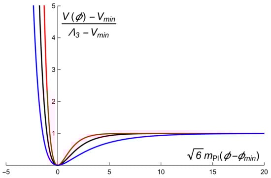
with $\mathrm{\Lambda }$ being constant. Several modifications and generalizations of this model have been proposed, such as the $\alpha$-attractor models [8,9,10], leading to power law inflation [11], or models with exponential power law inflation in modified gravity [12]. Some of these extensions (see for example [10] or [12]) can be written as particular cases of the potential

$$V\left(\varphi \right)={\mathrm{\Lambda }}_1{e}^{-\frac{\sqrt{6}\lambda }{m_{Pl}}\varphi }-{\mathrm{\Lambda }}_2{e}^{-\frac{\sqrt{6}\mu }{m_{Pl}}\varphi }+{\mathrm{\Lambda }}_3,$$

(4)

where ${\mathrm{\Lambda }}_j$, $j=1,2,3$, $\lambda$ and $\mu$ are positive coefficients with $\lambda >\mu$. In particular, by setting in $\mu =\frac{\lambda }{2}=\frac{1}{3}$, ${\mathrm{\Lambda }}_1={\mathrm{\Lambda }}_3=\frac{{\mathrm{\Lambda }}_2}{2}={\mathrm{\Lambda }}^4$, the potential (4) reduces to (3). Figure 1 shows the graphic of the potential (4) for several values of the parameters.

Figure 1. Graphics of the potential (4) for $\lambda =\frac{2}{3}$ (corresponding to the Starobinski model (3)) and $\mu$ taking the values $\frac{1}{3}$ (black line, also corresponding to the Starobinski model), $0.65$ (red line) and $0.15$ (blue line). The axes origin is $({\varphi }_{min},V_{min})$ with ${\varphi }_{min}$ being the inflaton value at which the potential takes its minimum and $V_{min}:=V\left({\varphi }_{min}\right)$.

In this work we use the Hamilton-Jacobi formalism to determine asymptotic solutions of the model (4) for two different situations: the kinetic dominance (KD) and the slow-roll (SR) stages.

The KD stage [13,14,15] is the period when the kinetic energy of the inflaton field dominates over its potential energy.

$${\dot{\varphi }}^2\gg V\left(\varphi \right).$$

(5)

It is a non-inflationary or pre-inflationary stage that is followed by a short fast-roll inflation phase [16] and afterwards by the traditional SR inflation stage [5,17,18,19,20,21,22,23,24]. Recently, Handley et al [14,15,25,26,27] have shown the relevance of the KD period (5) for setting initial conditions. Indeed, as it was stablished in [14,16], for models with a smooth and positive potential V the Hubble parameter is a positive monotonically decreasing function of t. As a consequence, the functions $\varphi \left(t\right)$ and $H\left(t\right)$ corresponding to arbitrary finite initial data are not singular forward in t. Nevertheless they may develop singularities backwards in t. Thus, it can be proved [14] that for generic initial conditions the evolution backwards in time starts by a KD regime followed by an inflationary regime.

The solutions of Equation (1) manifest generically branch point singularities of logarithmic type related to the condition (5), and their presence is associated with the so-called psi-series [28] asymptotic solutions. Handley et al. developed in [15] a general method to compute psi-series expansions for the solutions of Equation (1) and the generalization of Equation (2) for FLRW spacetimes with curvature. They referred to their series as logolinear series. As it was discussed in Section 2-C of [16], the mathematical singularity $t=t^{*}$ does not mean a real physical phenomenon. It is an extrapolation of the classical treatment of the inflaton models which is outside the validity region of the classical treatment. At this point quantum cosmology has to be used.

In a previous work [29] we have presented an alternative method for computing expansions of the solutions of (1)–(2) in the KD stage for wide classes of potentials. The starting point of the method is the Hamilton-Jacobi formalism, we look for solutions of the Hamilton-Jacobi equations as psi-series in $e^{\phi }$ ($\phi$ is the rescaled inflaton field $\phi \equiv \sqrt{\frac{3}{2}}\frac{\varphi }{m_{Pl}}$) with polynomial coefficients. The potential (4) is not a particular case of the models studied in [29], nevertheless we extend here our previous method by considering polynomial coefficients depending on the two variables $e^{-2\lambda \phi }$ and $e^{-2\mu \phi }$. We refer to these series as expolinear series. At this point we need to impose the exponents $\lambda$, $\mu$ and the quotient $\frac{\lambda }{\mu }$ to be irrational numbers, however a simple limit operation shows that the results also apply to rational exponents.

On the other hand, the SR stage is the period in which the potential energy dominates over the kinetic energy

$${\dot{\varphi }}^2\ll V\left(\varphi \right).$$

(6)

It is known [19,30] that many inflationary models exhibit separatrix solutions, these solutions behave as “attractor solutions” in the sense that they determine the asymptotic behaviour of all the solutions of the model as the cosmic time t is large enough. In particular they provide us with asymptotic expansions in the Hamilton-Jacobi formalism for the SR stage. In [31], we have studied the existence of separatrix solutions and have discussed their asymptotic expansions for wide classes of inflationary models. The results of [31] imply that the potential model (4) has a separatrix solution defined for $\varphi >{\varphi }_{min}$ for all values of the parameters $\lambda$ and $\mu$, however, the existence of a separatrix solution defined for $\varphi <{\varphi }_{min}$ requires that the condition $\lambda <1$ is fulfilled.

The paper is organized as follows: In Section 2, we briefly introduce the Hamilton-Jacobi formalism for the model (4). Section 3 describes the method for determining psi-series solutions for the Hamilton-Jacobi equations. We defer to Appendix A the discussion of how to derive from our psi-series in the inflaton field $\phi$, the logolinear series for $\phi \left(t\right)$ involving integer and irrational powers of $(t-t^{*})$. We devote Section 4 to obtain asymptotic expansions of the separatrix solutions. The question of how to use the series solutions obtained in Section 3 and Section 4 to provide suitable approximations to the Hamilton-Jacobi equations in the KD and SR stages is discussed in Section 5.1.

These approximations are applied in Section 5.2 to provide analytical approximations of several relevant quantities. Note that we need to take the parameter ${\mathrm{\Lambda }}_3$ in (4) as

$${\mathrm{\Lambda }}_3={\mathrm{\Lambda }}_1\left(\frac{\lambda }{\mu }-1\right){\left(\frac{{\mathrm{\Lambda }}_2\mu }{{\mathrm{\Lambda }}_1\lambda }\right)}^{\frac{\lambda }{\lambda -\mu }},$$

(7)

so that it is satisfied that $V_{min}=0$ and consequently, the model exhibits solutions which leave the inflation period and overlap a reheating phase [5,6,21,32,33,34]. Thus, we use the psi-series to determine the value of the inflaton field at the initial moment of the inflation period, and the separatrices to obtain the value of the inflaton field at the end of the inflation period. Using both approximations we provide a formula for the amount of inflation. The paper ends with a summary of conclusions in Section 6.

2. Hamilton Jacobi Formulation

Let us begin with the Hamilton Jacobi formulation of the inflationary models (1) and (2). We use the rescaled variables

$$\phi =\sqrt{\frac{3}{2}}\frac{\varphi }{m_{Pl}},v\left(\phi \right)=\frac{3}{m_{Pl}^2}V\left(\varphi \right),h=3H,$$

(8)

and rewrite equations (1) and (2) as

$$\ddot{\phi }+h\dot{\phi }+\frac{1}{2}{v}^{\prime }\left(\phi \right)=0,$$

(9)

and

$$h^2={\dot{\phi }}^2+v\left(\phi \right),$$

(10)

respectively, where

$$v\left(\phi \right)=c_1{e}^{-2\lambda \phi }-c_2{e}^{-2\mu \phi }+c_3,$$

(11)

with $c_j=\frac{3}{m_{Pl}^2}{\mathrm{\Lambda }}_j$, $j=1,2,3$. Furthermore, due to (7) the parameter $c_3$ is defined as

$$c_3=c_1\left(\frac{\lambda }{\mu }-1\right){\left(\frac{c_2\mu }{c_1\lambda }\right)}^{\frac{\lambda }{\lambda -\mu }}.$$

(12)

In this work we use Plank units $(G=c=\hslash =1)$. Thus, for the Starobinski model (3) we have that (see for example [15]) ${\mathrm{\Lambda }}^4={10}^{-10}{m}_{Pl}^2$, so the coefficients $c_j$, $j=1,2,3$ are of order ${10}^{-10}$.

2.1. The Hamilton-Jacobi Equations

In the Hamilton-Jacobi formulation of inflationary models the reduced Hubble parameter is determined as a function $h\left(\phi \right)$ of the inflaton field, consequently, we consider two subsets in the phase space $(\phi ,\dot{\phi })$ where $\dot{\phi }$ has a constant sign.

$$D_{+}=\left\{(\phi ,\dot{\phi }):\phi \ge {\phi }_{min},\dot{\phi }<0\right\},D_{-}=\left\{(\phi ,\dot{\phi }):\phi \le {\phi }_{min},\dot{\phi }>0\right\}.$$

(13)

The diffeomorphims

$$T_{+}:D_{+}\mapsto R_{+}:=\{(\phi ,h)\in {\mathbb{R}}^2:\phi \ge {\phi }_{min},\sqrt{v\left(\phi \right)}<h<+\infty \}$$

defined as

$$T_{+}(\phi ,\dot{\phi })=\left(\phi ,\sqrt{{\dot{\phi }}^2+v\left(\phi \right)}\right),T_{+}^{-1}(\phi ,h)=\left(\phi ,-\sqrt{h^2-v\left(\phi \right)}\right),$$

(14)

and

$$T_{-}:D_{-}\mapsto R_{-}:=\{(\phi ,h)\in {\mathbb{R}}^2:\phi \le {\phi }_{min},\sqrt{v\left(\phi \right)}<h<+\infty \},$$

where

$$T_{-}(\phi ,\dot{\phi })=\left(\phi ,\sqrt{{\dot{\phi }}^2+v\left(\phi \right)}\right),T_{-}^{-1}(\phi ,h)=\left(\phi ,\sqrt{h^2-v\left(\phi \right)}\right),$$

(15)

enable us to describe the dynamics of (9)–(10) on the regions $R_{\pm }$ of the $(\phi ,h)$ plane (see Figure 2 below).

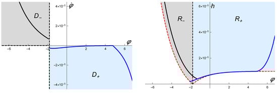
Figure 2. Regions $D_{\pm }$ in the left plot and $R_{\pm }$ in the right one. The black lines are representative trajectories with initial condition in $D_{-}$ (left) and $R_{-}$ (right). Analogously, the blue lines are representative trajectories with initial conditions in $D_{+}$ (left) and $R_{+}$ (right). The parameters of the model are taken as $\lambda =\frac{\sqrt{2}}{3}$, $\mu =\frac{\sqrt{3}}{4}$, $c_1=2\times {10}^{-10}$, $c_2=2.5\times {10}^{-10}$.

From Equations (9) and (10) it follows that

$$\dot{h}=-{\dot{\phi }}^2.$$

(16)

Thus, the parts of each solution $\phi \left(t\right)$ of (9) in $D_{\pm }$ satisfy the equations

$$h^{\prime }{\left(\phi \right)}^2=h{\left(\phi \right)}^2-v\left(\phi \right),$$

(17)

and

$$\dot{\phi }=-h^{\prime }\left(\phi \right),$$

(18)

Here primes denote derivatives with respect to $\phi$ and the reduced Hubble function h is assumed to be the positive root

$$h={\left({\dot{\phi }}^2+v\left(\phi \right)\right)}^{1/2}.$$

(19)

Equations (17) and (18) are referred to as the Hamilton-Jacobi formalism for inflationary models [6,19,35,36].

The sets $R_{\pm }$ plays the role of the phase space of the formalism. Thus each solution $h=h\left(\phi \right)$ of (17) determines a corresponding implicit solution $\phi \left(t\right)$ of (18) given by

$$t=-{\int }_{\phi \left(0\right)}^{\phi \left(t\right)}\frac{d\phi }{h^{\prime }\left(\phi \right)}.$$

(20)

2.2. The KD Period. Asymptotic Solutions

As a consequence of (16), it follows that the reduced Hubble parameter h is a positive monotonically decreasing function of t. This property implies that for smooth and positive potential functions v, the solutions $\phi \left(t\right)$ of (9) with arbitrary finite initial data do not have singularities forward in the cosmic time t. Nevertheless, the function $h\left(t\right)$ increases without bound backwards in time, so that we may expect that $h\left(t\right)$ and $\phi \left(t\right)$ may develop singularities. Thus, if the KD condition (5) holds then we may neglect v and $v^{\prime }$ in the inflaton equations and from (9) we have

$$\ddot{\phi }+\left|\dot{\phi }\right|\dot{\phi }\sim 0,$$

(21)

and we obtain two families of approximate solutions

$$\phi \sim \mp log(t-t^{*})+{\phi }_{p}ast\to {\left(t^{*}\right)}^{+},$$

(22)

where $t^{*}$ and ${\phi }_p$ are arbitrary constants. Consequently, the asymptotic form of the reduced Hubble parameter (19) is

$$h\sim \frac{1}{(t-t^{*})}ast\to {\left(t^{*}\right)}^{+}.$$

(23)

These approximate solutions of the inflaton equations are the dominant terms of the psi series expansions that we will consider below. The corresponding approximate solutions of (17) take the form

$$h\sim \frac{e^{\pm \phi }}{b}\mathrm{as}\phi \to \pm \infty ,$$

(24)

where b is an arbitrary strictly positive parameter ($b=e^{\pm {\phi }_p}$). We will denote by $h^{(+)}\left(\phi \right)$ the solutions of (17) which emerge from the KD region with asymptotic behaviour

$$h^{(+)}\left(\phi \right)\sim \frac{e^{\phi }}{b}\mathrm{as}\phi \to \infty .$$

(25)

Note that $h^{(+)}\left(\phi \right)$ is indeed solution of the equation

$$h^{\prime }=\sqrt{h^2-v\left(\phi \right)}.$$

(26)

We also use the notation ${\phi }^{(+)}\left(t\right)$ for the associated solution of (18) which blows up at a finite time $t^{*}$ given by

$$t^{*}=-{\int }_{\phi \left(0\right)}^{\infty }\frac{d\phi }{{\left(h^{(+)}\right)}^{\prime }\left(\phi \right)}.$$

(27)

and denote ${\mathrm{h}}^{(+)}\left(t\right)=h^{(+)}\left({\phi }^{(+)}\left(t\right)\right).$ The asymptotic forms of ${\phi }^{(+)}\left(t\right)$ and ${\mathrm{h}}^{(+)}\left(t\right)$ near the blow up time are given by

$${\phi }^{(+)}\left(t\right)\sim -log\left(\frac{t-t^{*}}{b}\right)ast\to {\left(t^{*}\right)}^{+},$$

(28)

and

$${\mathrm{h}}^{(+)}\left(t\right)\sim \frac{1}{t-t^{*}}ast\to {\left(t^{*}\right)}^{+}.$$

(29)

Analogously, we denote by $h^{(-)}\left(\phi \right)$ the solutions of (17) which emerge from the KD region with asymptotic behaviour

$$h^{(-)}\left(\phi \right)\sim \frac{e^{-\phi }}{b}\mathrm{as}\phi \to -\infty .$$

(30)

We point out that only if $\lambda <1$ the Equation (17) with potential (11) may admit solutions with asymptotic behaviour (30). Otherwise the potential function $v\left(\phi \right)$ is a dominant term with respect to $h{\left(\phi \right)}^2$ and $h^{\prime }{\left(\phi \right)}^2$ in (17) as $\phi \to -\infty$. We assume that $\lambda <1$, then it is clear that $h^{(-)}\left(\phi \right)$ is a solution of the equation

$$h^{\prime }=-\sqrt{h^2-v\left(\phi \right)}.$$

(31)

Now ${\phi }^{(-)}\left(t\right)$ stands for the associated solution of (18) which blows up at a finite time given by

$$t^{*}={\int }_{-\infty }^{\phi \left(0\right)}\frac{d\phi }{{\left(h^{(-)}\right)}^{\prime }\left(\phi \right)}.$$

(32)

and ${\mathrm{h}}^{(-)}\left(t\right)=h^{(-)}\left({\phi }^{(-)}\left(t\right)\right).$ The asymptotic behaviours of ${\phi }^{(-)}\left(t\right)$ and ${\mathrm{h}}^{(-)}\left(t\right)$ near the blow up time are given by

$${\phi }^{(-)}\left(t\right)\sim log\left(\frac{t-t^{*}}{b}\right)\mathrm{as}t\to {\left(t^{*}\right)}^{+},$$

(33)

and

$${\mathrm{h}}^{(-)}\left(t\right)\sim \frac{1}{t-t^{*}}\mathrm{as}t\to {\left(t^{*}\right)}^{+}.$$

(34)

2.3. Slow-Roll Stage and Separatrix Solutions

In our previous work [31] we proved that for a potential $v\left(\phi \right)$ such that

$$\underset{\phi \to \infty }{lim}\frac{v^{\prime }\left(\phi \right)}{2v\left(\phi \right)}=\alpha \mathrm{for}0\le \alpha <1,$$

(35)

the Equation (17) has a unique solution $h_s^{(+)}\left(\phi \right)$ satysfying

$$h_s^{(+)}\left(\phi \right)\sim \frac{\sqrt{v\left(\phi \right)}}{\sqrt{1-{\alpha }^2}}\mathrm{as}\phi \to \infty .$$

(36)

Furthermore, using the symmetry $\left(v\right(\phi ),h(\phi ),\phi (t\left)\right)\mapsto \left(v\right(-\phi ),h(-\phi ),-\phi (t\left)\right)$ of Equations (17) and (18), we have that provided

$$\underset{\phi \to -\infty }{lim}\frac{v^{\prime }\left(\phi \right)}{2v\left(\phi \right)}=-\beta \mathrm{for}0\le \beta <1,$$

(37)

the Equation (17) has a unique solution $h_s^{(-)}\left(\phi \right)$ such that

$$h_s^{(-)}\left(\phi \right)\sim \frac{\sqrt{v\left(\phi \right)}}{\sqrt{1-{\beta }^2}}\mathrm{as}\phi \to -\infty .$$

(38)

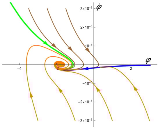
The trajectories in the $(\phi ,\dot{\phi })$ phase space associated to these solutions are boundaries of the regions filled by the solutions with asymptotic behaviour given by either (28) or (33) (see Figure 3 below). Moreover, $h_s^{(+)}\left(\phi \right)$ (resp. $h_s^{(-)}\left(\phi \right))$) is the boundary in the phase spaces $R^{+}$ (resp. $R^{-}$) between solutions of (17) defined for all $\phi >{\phi }_{min}$ (resp. $\phi <{\phi }_{min}$) and solutions of (17) which leave $R^{+}$ for a certain ${\phi }^{*}>{\phi }_{min}$ (resp. which leave $R^{-}$ for a certain ${\phi }^{*}<{\phi }_{min}$). These important solutions are referred to as separatrix solutions and it turns out that, for wide sets of initial conditions, the solutions of the model reduce asymptotically to these special solutions [19,30]. Thus, they provide us with accurate approximations to the solutions in the SR stage.

Figure 3. Phase portrait of (9), (11), the blue and green lines stand for the separatrices, the orange lines plot trajectories associated to solutions satisfying (28) while the brown lines corresponds to solutions with asymptotic behaviour (33). The model parameter values are $\lambda =\frac{\sqrt{2}}{3}$, $\mu =\frac{\sqrt{3}}{4}$, $c_1=2\times {10}^{-10}$, $c_2=2.5\times {10}^{-10}$.

For the inflationary model with the generalized Starobinski potential (11) we have that

$$\underset{\phi \to \infty }{lim}\frac{v^{\prime }\left(\phi \right)}{2v\left(\phi \right)}=0\mathrm{and}\underset{\phi \to -\infty }{lim}\frac{v^{\prime }\left(\phi \right)}{2v\left(\phi \right)}=-\lambda .$$

(39)

Consequently, a separatrix solution arises with asymptotic behaviour

$$h_s^{(+)}\left(\phi \right)\sim \sqrt{v\left(\phi \right)}\mathrm{as}\phi \to \infty .$$

(40)

Furthermore, provided that $\lambda <1$ there is another separatrix solution such that

$$h_s^{(-)}\left(\phi \right)\sim \frac{\sqrt{v\left(\phi \right)}}{\sqrt{1-{\lambda }^2}}\mathrm{as}\phi \to -\infty .$$

(41)

2.4. The Amount of Inflation

The inflation period of the universe evolution is characterized by an accelerated universe expansion $\ddot{a}>0$. From the identity

$$\frac{\ddot{a}}{a}=\frac{1}{3m_{Pl}^2}\left(V\left(\varphi \right)-{\dot{\varphi }}^2\right),$$

(42)

it follows that this period is determined by the constraint

$${\dot{\varphi }}^2<V\left(\varphi \right).$$

(43)

Then, the inflation regions (43) in $R_{\pm }$ are characterized by

$$\sqrt{v}<h<\sqrt{\frac{3v}{2}}.$$

(44)

It is well known that a successful solution to the horizon and flatness cosmological problems requires that the amount of inflation

$$N={\int }_{{\varphi }_{in}}^{{\varphi }_{end}}\frac{H}{\dot{\varphi }}d\varphi =\frac{1}{3}{\int }_{{\phi }_{end}}^{{\phi }_{in}}\frac{h}{h^{\prime }}d\phi ,$$

(45)

should be close to $N\sim 60$ [6,37,38,39]. Thus, given a solution $h=h\left(\phi \right)$ of (17) it is essential to determine the values ${\phi }_{in}$, ${\phi }_{end}$ for which inflation starts and ends. Now, due to (44) both values satisfy

$$h\left(\phi \right)=\sqrt{\frac{3v\left(\phi \right)}{2}}.$$

(46)

As we will show in Section 5.2, we obtain faithful approximations of ${\phi }_{in}$ if we use KD approximations for $h\left(\phi \right)$ in (46) supplied by appropriately truncated psi-series expansions. Moreover, ${\phi }_{end}$ is accurately approximated in terms of the SR approximations determined through separatrix expansions. Both approximations will be applied to determine the amount of inflation N as a function of the free parameter b.

3. Expolinear Series for the Reduced Hubble Parameter $\mathit{h}\left(\mathbf{\phi }\right)$ in the KD Period

We consider the KD period and look for solutions of (17) with asymptotic behaviour (25). Thus we substitute the psi-series expansion

$$h^{(+)}\left(\phi \right)=\frac{e^{\phi }}{b}+\sum _{n=1}^{\infty }{b}^{2n-1}{\gamma }_n^{(+)}\left(c_1{e}^{-2\lambda \phi },c_2{e}^{-2\mu \phi }\right)e^{-(2n-1)\phi },$$

(47)

in (17), where ${\gamma }_n^{(+)}\left(\phi \right)$ are polynomials on $c_1{e}^{-2\lambda \phi }$ and $c_2{e}^{-2\mu \phi }$. By inserting (47) into (17) we obtain

$$\begin{array}{c}{\displaystyle \sum _{n=1}^{\infty }}{b}^{2n-1}\left[\lambda x{\gamma }_{n,x}^{(+)}+\mu y{\gamma }_{n,y}^{(+)}+n{\gamma }_n^{(+)}\right]e^{-(2n-2)\phi }-\hfill \\ \\ -{\displaystyle \sum _{n=2}^{\infty }}{b}^{2n-2}\left[{\displaystyle \sum _{j+k=n,j,k\ge 1}}\right((\lambda x{\gamma }_{j,x}^{(+)}+\mu y{\gamma }_{j,y}^{(+)}+(j-\frac{1}{2}){\gamma }_j^{(+)})(\lambda x{\gamma }_{k,x}^{(+)}-\mu y{\gamma }_{k,y}^{(+)}+(k-\frac{1}{2}){\gamma }_k^{(+)})\hfill \\ \\ -\frac{1}{4}{\gamma }_j^{(+)}{\gamma }_k^{(+)}\left)\right]e^{-(2n-2)\phi }=\frac{1}{4}(x-y+c_3),\hfill \end{array}$$

(48)

where we have introduced the variables

$$x:=c_1{e}^{-2\lambda \phi },y:=c_2{e}^{-2\mu \phi }.$$

(49)

Henceforth, we will assume that

$$\lambda ,\mu \mathrm{and}\frac{\lambda }{\mu }\mathrm{are} \mathrm{irrational} \mathrm{numbers}.$$

(50)

Nevertheless a simple limit operation shows that the results below also apply to rational exponents, or irrational exponents $\lambda$ and $\mu$ such that $\lambda /\mu$ is rational. From (50) we have that the powers of x, y and $e^{-\phi }$ are linearly independent functions; consequently we may identify the coefficients of $e^{-2n\phi }$ for $n=0,1,\dots$ on both sides of Equation (48). Thus, for $n=0$ we obtain that ${\gamma }_1^{(+)}$ verifies the linear first order PDE

$$\lambda x{\gamma }_{1,x}^{(+)}+\mu y{\gamma }_{1,y}^{(+)}+{\gamma }_1^{(+)}=\frac{1}{4}(x-y+c_3),$$

(51)

which can be solved by the characteristic method [40] and, after the change of variables

$$\xi =y{x}^{-\frac{\mu }{\lambda }},\eta =x.$$

(52)

it reduces to the linear first order ordinary differential equation

$${\gamma }_{1,\eta }^{(+)}+\frac{1}{\lambda \eta }{\gamma }_1^{(+)}=\frac{1}{4\lambda }\left(1-\xi {\eta }^{\frac{\mu }{\lambda }-1}+c_3{\eta }^{-1}\right),$$

whose general solution is

$${\widehat{\gamma }}_1^{(+)}(\xi ,\eta )=P_1\left(\xi \right){\eta }^{-\frac{1}{\lambda }}+\frac{1}{4(1+\lambda )}\eta -\frac{1}{4(1+\mu )}\xi {\eta }^{\frac{\mu }{\lambda }}+\frac{c_3}{4},$$

where $P_1$ is an arbitrary function. In terms of the variables $(x,y)$, the general solution can be written as

$${\widehat{\gamma }}_1^{(+)}(x,y)=P_1\left(y{x}^{-\frac{\mu }{\lambda }}\right)x^{-\frac{1}{\lambda }}+\frac{x}{4(1+\lambda )}-\frac{y}{4(1+\mu )}+\frac{c_3}{4}.$$

Thus, Equation (51) has a unique polynomial solution given by

$${\gamma }_1^{(+)}(x,y)=\frac{x}{4(1+\lambda )}-\frac{y}{4(1+\mu )}+\frac{c_3}{4}.$$

(53)

Furthermore, identifying the coefficients of $e^{-2n\phi }$, $n\in \mathbb{N}$ in both sides of Equation (48) leads to the recursion relation

$$\begin{array}{c}\lambda x{\gamma }_{n+1,x}^{(+)}+\mu y{\gamma }_{n+1,y}^{(+)}+(n+1){\gamma }_{n+1}=\hfill \\ \\ {\displaystyle \sum _{j+k=n+1,j,k\ge 1}}[(\lambda x{\gamma }_{j,x}^{(+)}+\mu y{\gamma }_{j,y}^{(+)}+(j-\frac{1}{2}){\gamma }_j^{(+)})(\lambda x{\gamma }_{k,x}^{(+)}+\mu y{\gamma }_{k,y}^{(+)}+(k-\frac{1}{2}){\gamma }_k^{(+)})\hfill \\ \\ -\frac{1}{4}{\gamma }_j^{(+)}{\gamma }_k^{(+)}].\hfill \end{array}$$

(54)

The Equations (54) are nonhomogeneous linear first order PDE, whose nonhomogeneous terms depend on the coefficients ${\gamma }_j^{(+)}$ with $j=1,\dots ,n$. We now use induction to prove that the coefficients ${\gamma }_n^{(+)}(x,y)$ in Equation (47) are recursively determined from Equation (54) as polynomials of degree n on $(x,y)$ i.e.

$${\gamma }_n^{(+)}(x,y)=\sum _{j+k\le n}{\gamma }_{n,j,k}^{(+)}{x}^j{y}^k.$$

(55)

From Equation (53) we have that ${\gamma }_1^{(+)}$ is of the form (55) with

$${\gamma }_{1,0,0}^{(+)}=\frac{c_3}{4},{\gamma }_{1,1,0}^{(+)}=\frac{1}{4(1+\lambda )},{\gamma }_{1,0,1}^{(+)}=-\frac{1}{4(\mu +1)}.$$

(56)

By using the induction hypothesis, we can write the right-hand side of Equation (54) as

$$\sum _{j+k\le n+1}{q}_{n+1,j,k}^{(+)}{x}^j{y}^k,$$

(57)

where the coefficients $q_{n+1,j,k}^{(+)}$ depend on ${\gamma }_{l,j,k}^{(+)}$ for $l=1,\dots ,n$ and $j,k$ such that $j+k\le l$. The change of variables (52) transforms (54) and (57) into

$${\gamma }_{n+1,\eta }^{(+)}+\frac{n+1}{\lambda \eta }{\gamma }_{n+1}^{(+)}=\frac{1}{\lambda }\sum _{j+k\le n+1}{q}_{n+1,j,k}^{(+)}{\xi }^k{\eta }^{j+\frac{\mu }{\lambda }k-1}.$$

with general solution

$${\widehat{\gamma }}_{n+1}^{(+)}(\xi ,\eta )=P_{n+1}\left(\xi \right){\eta }^{-\frac{n+1}{\lambda }}+\sum _{j+k\le n+1}\frac{q_{n+1,j,k}^{(+)}}{j\lambda +k\mu +(n+1)}{\xi }^k{\eta }^{j+\frac{\mu }{\lambda }k}.$$

Here $P_{n+1}$ denotes an arbitrary function on $\xi$. Thus, in terms of the variables $(x,y)$ the unique polynomial solution of Equation (54) is given by

$${\gamma }_{n+1}^{(+)}(x,y)=\sum _{j+k\le n+1}\frac{q_{n+1,j,k}^{(+)}}{j\lambda +k\mu +(n+1)}{x}^j{y}^k.$$

(58)

For example, we have that the first Equation (54) are

$$\begin{array}{ccc}\lambda x{\gamma }_{2,x}^{(+)}+\mu y{\gamma }_{2,y}^{(+)}+2{\gamma }_2^{(+)}\hfill & =\hfill & {\left(\lambda x{\gamma }_{1,x}^{(+)}+\mu y{\gamma }_{1,y}^{(+)}+\frac{1}{2}{\gamma }_1^{(+)}\right)}^2-\frac{1}{4}{\left({\gamma }_1^{(+)}\right)}^2,\hfill \\ \\ \lambda x{\gamma }_{3,x}^{(+)}+\mu y{\gamma }_{3,y}^{(+)}+3{\gamma }_3^{(+)}\hfill & =\hfill & 2\left(\lambda x{\gamma }_{1,x}^{(+)}+\mu y{\gamma }_{1,y}^{(+)}+\frac{1}{2}{\gamma }_1^{(+)}\right)\left(\lambda x{\gamma }_{2,x}^{(+)}+\mu y{\gamma }_{2,y}^{(+)}+\frac{3}{2}{\gamma }_2^{(+)}\right)\hfill \\ \\ & & -\frac{1}{2}{\gamma }_1^{(+)}{\gamma }_2^{(+)},\hfill \end{array}$$

(59)

and the second coefficient in (47) is given by

$$\begin{array}{ccc}{\gamma }_2^{(+)}(x,y)\hfill & =\hfill & \frac{\lambda x^2}{32{(1+\lambda )}^2}+\frac{xy(\lambda +\mu +2\lambda \mu )}{16(1+\lambda )(1+\mu )(2+\lambda +\mu )}\hfill \\ \\ \hfill & \hfill & +\frac{\mu y^2}{32{(1+\mu )}^2}+\frac{c_3\lambda x}{16(1+\lambda )(2+\lambda )}+\frac{c_3\mu y}{16(1+\mu )(2+\mu )}.\hfill \end{array}$$

(60)

Recalling Equations (47), (49) and (55) we get that the reduced Hubble parameter is

$$h^{(+)}\left(\phi \right)=\frac{e^{\phi }}{b}+\sum _{n=1}^{\infty }\sum _{j+k\le n}{b}^{2n-1}{\gamma }_{n,j,k}^{(+)}{c}_1^j{c}_2^k{e}^{(-2j\lambda -2k\mu -2n+1)\phi }.$$

(61)

On the other hand, if $\lambda <1$ we can use the symmetry $\left(v\right(\phi ),h(\phi ),\phi (t\left)\right)\to \left(v\right(-\phi )$, $h(-\phi ),-\phi \left(t\right))$ of Equations (17) and (18) to find that the psi-series corresponding to solutions with asymptotic behaviour (30) are given by

$$h^{(-)}\left(\phi \right)=\frac{e^{-\phi }}{b}+\sum _{n=1}^{\infty }\sum _{j+k\le n}{b}^{2n-1}{\gamma }_{n,j,k}^{(-)}{c}_1^j{c}_2^k{e}^{(-2j\lambda -2k\mu +2n-1)\phi }.$$

(62)

where

$${\gamma }_{n,j,k}^{(-)}={\gamma }_{n,j,k}^{(+)}{|}_{\lambda \to -\lambda ,\mu \to -\mu }n\in \mathbb{N},j=0,\dots ,n,k=0,\dots ,n-j.$$

(63)

Note that as $0<\mu <\lambda <1$ we have for the exponents in (62) that $-2j\lambda -2k\mu +2n-1>-2(j+k)\lambda +2n-1>-1$ and consequently the terms in the sum are subdominant with respect to $e^{-\phi }$ as $\phi \to -\infty$.

4. Asymptotic Series for Separatrix Solutions

In this section we determine asymptotic expansions for the separatrix solutions of Equation (17). According to (36) the solution $h_s^{(+)}\left(\phi \right)$ of (17) satisfies

$$h_s^{(+)}\left(\phi \right)\sim \sqrt{v\left(\phi \right)}\sim \sqrt{c_3}\left(1-\frac{c_2}{2c_3}{e}^{-2\mu \phi }+\frac{c_1}{2c_3}{e}^{-2\lambda \phi }+...\right),\phi \to \infty .$$

(64)

where the dots stand for lower order terms as $\phi \to \infty$. We next prove that the asymptotic expansion for the separatrix solution is of the form

$$h_s^{(+)}\left(\phi \right)=\sqrt{c_3}\sum _{n=0}^{\infty }\sum _{l=0}^{\infty }{S}_{n,l}{c}_1^n{c}_2^l{c}_3^{-n-l}{e}^{-2n\lambda \phi }{e}^{-2l\mu \phi },$$

(65)

where the coefficients $S_{n,l}$ can be recursively determined. Equivalently, in terms of the variables $(x,y)$ (49) we have

$$h_s^{(+)}\left(\phi \right)=\sqrt{c_3}\sum _{n=0}^{\infty }\sum _{l=0}^{\infty }{S}_{n,l}{c}_3^{-n-l}{x}^n{y}^l.$$

(66)

Substitution of (66) into (17) leads us to the equation

$$\begin{array}{c}{\displaystyle \sum _{n=0}^{\infty }}{\displaystyle \sum _{l=0}^{\infty }}{c}_3^{1-n-l}\left({\displaystyle \sum _{j=0}^n}{\displaystyle \sum _{k=0}^l}[4(j\lambda +k\mu )((n-j)\lambda +(l-k)\mu )-1]S_{j,k}{S}_{n-j,l-k}\right)x^n{y}^l\hfill \\ \\ =-x+y-c_3.\hfill \end{array}$$

(67)

Since the powers of x and y are linearly independent, we can identify the coefficient of each monomial $x^n{y}^l$ in both sides of Equation (67). For example, by setting $(n,l)=(0,0)$, $(1,0)$ and $(0,1)$, it follows that

$$S_{0,0}=1,S_{1,0}=\frac{1}{2},S_{0,1}=-\frac{1}{2},$$

(68)

which is in agreement with (64). On the other hand, if $(n,l)\notin \left\{\right(0,0),(1,0),(0,1\left)\right\}$, equating the coefficient of $x^n{y}^l$ in both sides of (67) provides us with

$$S_{n,l}=\frac{1}{2}\sum _{(j,k)\in {\mathcal{T}}_{n,l}}[4(j\lambda +k\mu )((n-j)\lambda +(l-k)\mu )-1]S_{j,k}{S}_{n-j,l-k},$$

(69)

where ${\mathcal{T}}_{n,l}=\{(j,k):0\le j\le n,0\le k\le l\}\setminus \{(0,0),(n,l)\}$. As a consequence, the Equations (68) and (69) supply a recursion formula to determine all the coefficients in (65).

Analogously, if we assume that $\lambda <1$, taking into account the asymptotic behaviour (41) of the separatrix solution $h_s^{(-)}\left(\phi \right)$ one finds

$$h_s^{(-)}\left(\phi \right)\sim \frac{\sqrt{v\left(\phi \right)}}{\sqrt{1-{\lambda }^2}}\sim \sqrt{\frac{c_1}{1-{\lambda }^2}}{e}^{-\lambda \phi }\left(1-\frac{c_2}{2c_1}{e}^{2(\lambda -\mu )\phi }+\frac{c_3}{2c_1}{e}^{2\lambda \phi }+\dots \right)\mathrm{for}\phi \to -\infty ,$$

(70)

where the dots stand for lower order terms. Then, we look for an expansion of the form

$$h_s^{(-)}\left(\phi \right)=\sqrt{\frac{1}{1-{\lambda }^2}}{x}^{\frac{1}{2}}\left[1+\sum _{n=1}^{\infty }{r}_n\left(y\right)x^{-n}\right],$$

(71)

where the coefficients $r_n\left(y\right)$ are polynomials in y. Substitution of (71) into (17) leads us to the equation

$$\begin{array}{c}{\displaystyle \sum _{n=1}^{\infty }}\left[2\lambda \mu y{r}_n^{\prime }-\left((2n-1){\lambda }^2+1\right)r_n\right]x^{1-n}=\frac{1}{2}(1-{\lambda }^2)(y-c_3)\hfill \\ \\ -\frac{1}{2}{\displaystyle \sum _{n=2}^{\infty }}\left({\displaystyle \sum _{j+k=n,j,k\ge 1}}\left[(2\mu y{r}_j^{\prime }-(2j-1)\lambda r_j)(2\mu y{r}_k^{\prime }-(2k-1)\lambda r_k)-r_j{r}_k\right]\right)x^{1-n}.\hfill \end{array}$$

(72)

As the powers of x and y are linearly independent, we can equate the coefficient of each power of x in both sides of (72). Thus, from the coefficient of $x^0$ we have that

$$2\lambda \mu r_1^{\prime }-({\lambda }^2+1)r_1=\frac{1}{2}(1-{\lambda }^2)(y-c_3).$$

(73)

The only polynomial solution of (73) is given by

$$r_1\left(y\right)=\frac{\left({\lambda }^2-1\right)y}{2\left({\lambda }^2-2\lambda \mu +1\right)}-\frac{c_3\left({\lambda }^2-1\right)}{2\left({\lambda }^2+1\right)}$$

(74)

The coefficient of $x^{1-n}$ with $n>1$ implies the equation

$$\begin{array}{c}2\lambda \mu y{r}_n^{\prime }-\left((2n-1){\lambda }^2+1\right)r_n=\hfill \\ \\ -\frac{1}{2}{\displaystyle \sum _{j+k=n,j,k\ge 1}}\left[(2\mu y{r}_j^{\prime }-(2j-1)\lambda r_j)(2\mu y{r}_k^{\prime }-(2k-1)\lambda r_k)-r_j{r}_k\right],n=2,3,\dots .\hfill \end{array}$$

(75)

We now use induction in n to prove that equations (75) determine recursively $r_n\left(y\right)$ as a polynomial of degree at most n. First, from (74) we have that $r_1\left(y\right)$ is a polynomial of degree 1 in y. Next, we have that the right hand sides of equations (75) depend only on $r_j$$j=\dots ,n-1$, moreover using the induction hypothesis, these terms are polynomials in y of degree less or equal than n. Consequently $r_n\left(y\right)$ is determined by (75) as a polynomial of degree at most n. For example, for $n=2$ (75) takes the form

$$2\lambda \mu r_2^{\prime }-(3{\lambda }^2+1)r_2=-2{\mu }^2{y}^2{\left(r_1^{\prime }\right)}^2+2\lambda \mu y{r}_1{r}_1^{\prime }+\frac{1}{2}(1-{\lambda }^2)r_1^2,$$

(76)

whose polynomial solution is

$$\begin{array}{ccc}{r}_2\left(y\right)\hfill & =\hfill & -\frac{c_3^2{\left({\lambda }^2-1\right)}^3}{8\left(-3{\lambda }^2-1\right){\left({\lambda }^2+1\right)}^2}+\frac{c_3{\left({\lambda }^2-1\right)}^2\left({\lambda }^2-2\lambda \mu -1\right)y}{4\left({\lambda }^2+1\right)\left({\lambda }^2-2\lambda \mu +1\right)\left(-3{\lambda }^2+2\lambda \mu -1\right)}\hfill \\ \\ & & -\frac{{\left({\lambda }^2-1\right)}^2\left({\lambda }^2-4\lambda \mu +4{\mu }^2-1\right)y^2}{8{\left({\lambda }^2-2\lambda \mu +1\right)}^2\left(-3{\lambda }^2+4\lambda \mu -1\right)}.\hfill \end{array}$$

(77)

In general, it can be written that

$$r_n\left(y\right)=\sum _{j=0}^n{r}_{n,j}{y}^j,$$

(78)

where the coefficients $r_{n,j}$ depend on $\lambda$, $\mu$ and $c_3$. In this way, the expansion of the separatrix solution $h_s^{(-)}\left(\phi \right)$ takes the form

$$h_s^{(-)}\left(\phi \right)=\sqrt{\frac{c_1}{1-{\lambda }^2}}\left[e^{-\lambda \phi }+\sum _{n=1}^{\infty }\sum _{j=0}^n{r}_{n,j}{e}^{\left[\right(2n-1)\lambda -2j\mu ]\phi }\right].$$

(79)

Note that as $\mu <\lambda$ the exponents in (79) satisfy $(2n-1)\lambda -2j\mu >-\lambda$ so the terms in the sum are subdominant terms with respect to $e^{-\lambda \phi }$ as $\phi \to -\infty$.

5. Aplications

In this section we apply the expansions obtained in Section 3 and Section 4 to get suitable approximations to the solutions of the Hamilton-Jacobi Equation (17) with $v\left(\phi \right)$ given by (11) in both the KD and the SR stages, as well as to the determination of the duration of the inflation period and the amount of inflation.

5.1. Approximate Solutions

We define the m-order approximation $h_{approx,m}^{(+)}(\phi ,b)$ to $h^{(+)}\left(\phi \right)$ (resp. $h_{s,approx,m}^{(+)}\left(\phi \right)$ to $h_s^{(+)}\left(\phi \right)$) as the truncated series (61) (resp. (65)) in which we keep all the terms in $e^{-c\phi }$ with $c\le m-1$ and remove the terms with $c>m-1$. Thus, as the expansion (61) for $h^{(+)}\left(\phi \right)$ contains terms in $e^{(-2j\lambda -2k\mu -2n+1)\phi }$ with j and k being greater than or equal than zero, only the terms with $n\le \left[\frac{m}{2}\right]$ determine the m-order approximation. Here $[.]$ stands for the integer part of a real number. More precisely, taking into account that $0\le j,k\le n$ and $j+k\le n$ it follows that

$$h_{approx,m}^{(+)}(\phi ,b)=\frac{e^{\phi }}{b}+\sum _{(n,j,k)\in I_m^{(+)}}{b}^{2n-1}{\gamma }_{n,j,k}^{(+)}{c}_1^j{c}_2^k{e}^{(-2j\lambda -2k\mu -2n+1)\phi },$$

(80)

where $I_m^{(+)}$ is the finite set of indeces

$$I_m^{(+)}:=\{(n,j,k):n\le \left[\frac{m}{2}\right],j+k\le n,j\lambda +k\mu \le \frac{m}{2}-n\}.$$

(81)

Analogously, the expansion (65) for $h_s^{(+)}\left(\phi \right)$ contains terms in $e^{-2(n\lambda +l\mu )\phi }$ with $n,l=1,\dots$ so that the corresponding m-order approximation is given by

$$h_{s,approx,m}^{(+)}\left(\phi \right)=\sqrt{c_3}\sum _{(n,l)\in I_{s,m}^{(+)}}{S}_{n,l}{c}_1^n{c}_2^l{c}_3^{-n-l}{e}^{-2n\lambda \phi }{e}^{-2l\mu \phi }.$$

(82)

where $I_{s,m}^{(+)}$ denotes the set

$$I_{s,m}^{(+)}=\{(n,l):n,l=0,1,\dots ,2n\lambda +2l\mu \le m-1\},$$

(83)

Figure 4 shows the 6-order approximations for $h^{(+)}\left(\phi \right)$ and $h_s^{(+)}\left(\phi \right)$ together with the numerical solution. We observe that $h_{approx,6}^{(+)}\left(\phi \right)$ represents a very good approximation in the KD region while $h_{s,approx,6}^{(+)}\left(\phi \right)$ gives a very good approximation in the SR region.

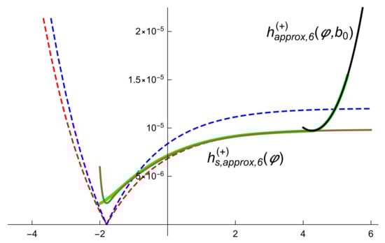
Figure 4. The green line shows the numerical solution of (17) with initial conditions ${\phi }_0=6$, $h_0=h_{approx,6}({\phi }_0,b_0)$ with $b_0=1.48\times {10}^7$. The black line shows the six order KD approximation $h_{approx,6}^{(+)}(\phi ,b_0)$. The brown line shows the six order approximation $h_{s,approx,6}\left(\phi \right)$ for the separatrix. The values of the parameters are $\lambda =\frac{\sqrt{2}}{3}$, $\mu =\frac{\sqrt{3}}{4}$, $c_1=2\times {10}^{-10}$, $c_2=2.5\times {10}^{-10}$. We notice that the green line (numerical approximation) overlappes the black line (KD approximation) in the KD region and overlappes the brown line (separatrix approximation) in the SR region. The region between the blue and red dotted lines is the inflation region.

To get suitable approximations of $h^{(-)}\left(\phi \right)$ and $h_s^{(-)}\left(\phi \right)$ for $\lambda <1$, we can proceed in a similar way. Thus we define the m-order approximation $h_{approx,m}^{(-)}(\phi ,b)$ to $h^{(-)}\left(\phi \right)$ (resp. $h_{s,approx,m}^{(-)}\left(\phi \right)$ to $h_s\left(\phi \right)$) as the truncated series (62) (resp. (79) in which we keep the terms in $e^{c\phi }$ for $c\le m-1$ and remove the terms with $c>m-1$. The expansion (62) for $h^{(-)}\left(\phi \right)$ contains terms in $e^{(-2j\lambda -2k\mu +2n-1)\phi }$ for $n=1,\dots$, $j,k,\le n$, thus by recalling that $0<\mu <\lambda <1$, it is clear that

$$n-j\lambda -k\mu >n-(j+k)\lambda \ge n(1-\lambda ),$$

and consequently, only terms with $n\le \left[\frac{m}{2(1-\lambda )}\right]$ determine the m-order approximation. More precisely,

$$h_{approx,m}^{(-)}(\phi ,b)=\frac{e^{-\phi }}{b}+\sum _{(n,j,k)\in I_m^{(-)}}{b}^{2n-1}{\gamma }_{n,j,k}^{(-)}{c}_1^j{c}_2^k{e}^{(-2j\lambda -2k\mu +2n-1)\phi }.$$

(84)

with $I_m^{(-)}$ being the finite set of indeces

$$I_m^{(-)}:=\{(n,j,k):n\le \left[\frac{m}{2(1-\lambda )}\right],j+k\le n,j\lambda +k\mu \ge n-\frac{m}{2}\}.$$

(85)

Analogously, the expansion (79) of $h_s^{(-)}\left(\phi \right)$ contains terms in $e^{\left[\right(2n-1)\lambda -2j\mu ]\phi }$ for $n=1,\dots$ and $j=0,\dots ,n$. Then, as

$$(2n-1)\lambda -2j\mu \ge 2n(\lambda -\mu )-\lambda ,$$

the m-order approximation $h_{s,approx,m}^{(-)}\left(\phi \right)$ only contains terms with $n\le \left[\frac{m+\lambda -1}{2(\lambda -\mu )}\right]$. Thus,

$$h_{s,approx,m}^{(-)}\left(\phi \right)=\sqrt{\frac{c_1}{1-{\lambda }^2}}\left[e^{-\lambda \phi }+\sum _{(n,j)\in I_{s,m}^{(-)}}{r}_{n,j}{e}^{\left[\right(2n-1)\lambda -2j\mu ]\phi }\right].$$

(86)

with $I_{s,m}^{(-)}$ being the finite set of indeces

$$I_{s,m}^{(-)}=\{(n,j):0\le n\le \left[\frac{m+\lambda -1}{2(\lambda -\mu )}\right],0\le j\le n,(2n-1)\lambda -2j\mu \le m-1\}.$$

(87)

In order to compare the approximations $h_{approx,m}^{(-)}(\phi ,b)$ and $h_{s,approx,m}^{(-)}\left(\phi \right)$ with a numerical solution $h^{(-)}\left(\phi \right)$ it is convenient to use the modified Hubble parameter

$$\mathfrak{h}\left(\phi \right):=\frac{h\left(\phi \right)}{\sqrt{v\left(\phi \right)}}.$$

(88)

In terms of $\mathfrak{h}=\mathfrak{h}\left(\phi \right)$, the Equation (31) reads

$${\mathfrak{h}}^{\prime }=-\sqrt{{\mathfrak{h}}^2-1}-\mathfrak{v}\mathfrak{h},$$

(89)

where

$$\mathfrak{v}:=\frac{v^{\prime }\left(\phi \right)}{2v\left(\phi \right)}.$$

(90)

The Equation (89) allows us to avoid the numerical instabilities due to the exponential growth of the solutions of (31) as $\phi \to -\infty$. Figure 5 shows the graphics of $h_{approx,6}^{(-)}(\phi ,b)/\sqrt{v\left(\phi \right)}$ and $h_{s,approx,6}^{(-)}\left(\phi \right)/\sqrt{v\left(\phi \right)}$ together with the numerical solution $\mathfrak{h}$ of (89). We point out that $h_{approx,6}^{(-)}(\phi ,b)/\sqrt{v\left(\phi \right)}$ provides a very good approximation in the KD region while $h_{s,approx,6}^{(-)}\left(\phi \right)/\sqrt{v\left(\phi \right)}$ provides a very good approximation in the SR region.

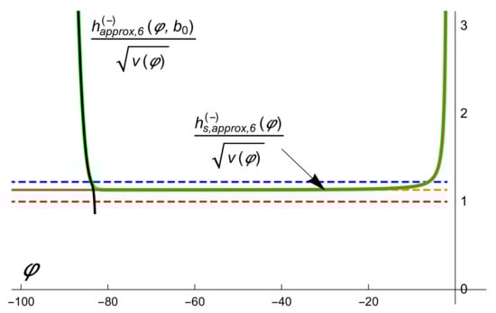
Figure 5. The green line shows the numerical solution of Equation (89) with initial conditions ${\phi }_0=-100$, ${\mathfrak{h}}_0=h_{approx,6}^{(-)}({\phi }_0,b_0)/\sqrt{v\left({\phi }_0\right)}$ with $b_0=2\times {10}^{24}$. The black line shows the six -order KD approximation $h_{approx,6}^{(-)}(\phi ,b_0)/\sqrt{v\left(\phi \right)}$. The brown line shows the sixth -order approximation $h_{s,approx,6}^{(-)}\left(\phi \right)/\sqrt{v\left(\phi \right)}$ to the separatrix. The orange dotted line corresponds to the asymptotic behaviour of the separatrix solution ${\mathfrak{h}}_s\left(\phi \right)\sim {(1-{\lambda }^2)}^{-1/2}$ as $\phi \to -\infty$. The values of the parameters are $\lambda =\frac{\sqrt{2}}{3}$, $\mu =\frac{\sqrt{3}}{4}$, $c_1=2\times {10}^{-10}$, $c_2=2.5\times {10}^{-10}$. We notice that the green line (numerical approximation) is overlapped by the black line (KD approximation) in the KD region and by the brown line (separatrix approximation) in the SR region. The region between the blue and red dotted lines is the inflation region.

It is worth noticing that in terms of the modified Hubble parameter the inflation region is given by

$$1<\mathfrak{h}<\sqrt{\frac{3}{2}},$$

and as we will show next, it takes place for $\phi$ along an interval about $(-100,0)$. Due to the exponential growth of $\sqrt{v\left(\phi \right)}$ as $\phi \to -\infty$, it is not possible to appreciate the inflation region (44) in the $(\phi ,h)$ plane.

5.2. Aplications to the Inflation Period

Let us now look for appropriate approximations to the values ${\phi }_{in}\left(b\right)$ and ${\phi }_{end}$ of the inflation period as well as to the amount of inflation $N\left(b\right)$. For a solution $h^{(+)}\left(\phi \right)$ of (17) satisfying (25), its m-order approximations $h_{approx,m}^{(+)}(\phi ,b)$ in the KD period allows us to get an approximate value of ${\phi }_{in}$ as a function of the parameter b through the equation

$$h_{approx,m}^{(+)}(\phi ,b)=\sqrt{\frac{3v\left(\phi \right)}{2}}.$$

(91)

On the other hand, as $h_{s,approx,m}^{(+)}\left(\phi \right)$ gives a suitable approximation for $h^{(+)}\left(\phi \right)$ in the SR stage, ${\phi }_{end}$ can be approximated by means of the equation

$$h_{s,approx,m}^{(+)}\left(\phi \right)=\sqrt{\frac{3v\left(\phi \right)}{2}}.$$

(92)

We denote the solutions of (91) and (92) by ${\phi }_{in,m}\left(b\right)$ and ${\phi }_{end,m}$, respectively. Then, to calculate $N\left(b\right)$ we need a value ${\phi }_m^{*}\left(b\right)$ such that the KD approximation holds for the interval $\phi \in ({\phi }^{*}\left(b\right),{\phi }_{in,m}\left(b\right))$, while the SR approximation holds for the remaining part of the inflation period. To this end, we choose the value of $\phi$ for which the function

$${\left(h_{approx,m}^{(+)}(\phi ,b)-h_{s,approx,m}^{(+)}\left(\phi \right)\right)}^2,$$

reaches its minimum. Thus, we can estimate the amount of inflation as a function of b as

$$\begin{array}{ccc}{N}_m\left(b\right)\hfill & \approx \hfill & \frac{1}{3}{\int }_{{\phi }_{end}}^{{\phi }_m^{*}\left(b\right)}{h}_{s,approx,m}^{(+)}\left(\phi \right){\left(\frac{d}{d\phi }{h}_{s,approx,m}^{(+)}\left(\phi \right)\right)}^{-1}d\phi \hfill \\ \\ \hfill & \hfill & +\frac{1}{3}{\int }_{{\phi }_m^{*}\left(b\right)}^{{\phi }_{in,m}\left(b\right)}{h}_{approx,m}^{(+)}(\phi ,b){\left(\frac{\partial }{\partial \phi }{h}_{approx,m}^{(+)}(\phi ,b)\right)}^{-1}d\phi .\hfill \end{array}$$

(93)

The approximation (93) can be used to select an appropriate value of the parameter b and, consequently, to determine the initial conditions, corresponding to a solution of Equation (17) with a previously fixed value of N.

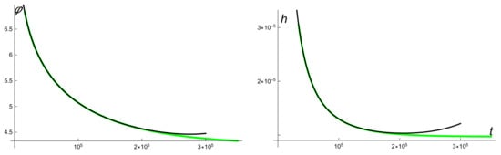
Figure 6 and Figure 7 illustrate the application of this method. The values for the parameters of the potential are the same as those chosen in Section 5.1 and we are using again the six-order approximations. In particular, for $N\left(b\right)=60$, we obtain $b_{60}\approx 2.28186\times {10}^7$ while for $N\left(b\right)=70$, we obtain $b_{70}\approx 2.80532\times {10}^7$. In Figure 7, we plot the numerical solution of (17) with initial conditions ${\phi }_0=12$, $h_0=h_{approx,6}^{(+)}({\phi }_0,b_{60})$ (left) and ${\phi }_0=12$, $h_0=h_{approx,6}^{(+)}({\phi }_0,b_{70})$ (right). Numerical computation of the amount of inflation for the solution leads to $N_{num}\approx 59.044$ and $N_{num}\approx 68.995$ respectively.

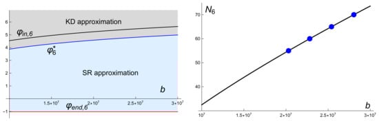
Figure 6. The left figure shows the graphs of the functions ${\phi }_{in,6}\left(b\right)$ (black line), ${\phi }_6^{*}\left(b\right)$ (blue line), and ${\phi }_{end,6}$ (red line) for the solutions (25) of (17) with potential (11) and $\lambda =\frac{\sqrt{2}}{3}$, $\mu =\frac{\sqrt{3}}{4}$, $c_1=2\times {10}^{-10}$, $c_2=2.5\times {10}^{-10}$. It also shows the regions in the $(b,\phi )$ plane corresponding to the KD approximation (gray region) and the SR approximation (blue region). The right figure shows the amount of the inflation $N_6\left(b\right)$. The blue dots indicate the values $N=55,60,65$, and 70.

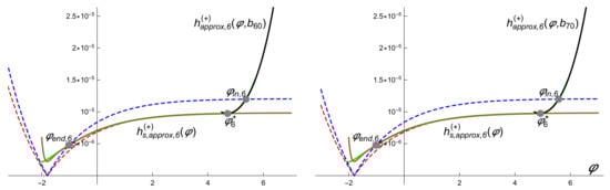
Figure 7. The green lines show the numerical solution $h^{(+)}\left(\phi \right)$ of (26) with initial conditions ${\phi }_0=12$, $h_0=h_{approx,6}^{(+)}({\phi }_0,b_{60})$ (left) and ${\phi }_0=12$, $h_0=h_{approx,6}^{(+)}({\phi }_0,b_{70})$ (right) for the model with potential (11) and $\lambda =\frac{\sqrt{2}}{3}$, $\mu =\frac{\sqrt{3}}{4}$, $c_1=2\times {10}^{-10}$, $c_2=2.5\times {10}^{-10}$. The black lines show the KD approximation $h_{approx,6}^{(+)}(\phi ,b_{60})$ (left) and $h_{approx,6}^{(+)}(\phi ,b_{70})$ (right) and the brown lines represent the SR approximation $h_{s,approx,6}^{(+)}\left(\phi \right)$. The regions between blue and red dotted lines are the inflation regions. The gray dots correspond (from right to left) to ${\phi }_{in,6}\left(b_{60}\right)$, ${\phi }_6^{*}\left(b_{60}\right)$ and ${\phi }_{end,6}$ (left) and ${\phi }_{in,6}\left(b_{70}\right)$, ${\phi }_6^{*}\left(b_{70}\right)$ and ${\phi }_{end,6}$ (right).

In the case $\lambda <1$ we can proceed in the same way for solutions $h^{(-)}\left(\phi \right)$ of (17) with asymptotic behaviour (30). For these solutions ${\phi }_{in,m}\left(b\right)$ and ${\phi }_{end.m}\left(b\right)$ are taken as the solutions of the equations

$$h_{approx,m}^{(-)}(\phi ,b)=\sqrt{\frac{3v\left(\phi \right)}{2}},h_{s,approx,m}^{(-)}\left(\phi \right)=\sqrt{\frac{3v\left(\phi \right)}{2}}.$$

The value ${\phi }_m^{*}\left(b\right)$ is taken as the minimum of the function

$${\left(h_{approx,m}^{(+)}(\phi ,b)-h_{s,approx,m}^{(+)}\left(\phi \right)\right)}^2,$$

and the amount of inflation is estimated by

$$\begin{array}{ccc}{N}_m\left(b\right)\hfill & \approx \hfill & \frac{1}{3}{\int }_{{\phi }_m^{*}\left(b\right)}^{{\phi }_{in,m}\left(b\right)}{h}_{approx,m}^{(-)}(\phi ,b){\left(\frac{\partial }{\partial \phi }{h}_{approx,m}^{(-)}(\phi ,b)\right)}^{-1}d\phi \hfill \\ \\ \hfill & \hfill & +\frac{1}{3}{\int }_{{\phi }_{end}}^{{\phi }_m^{*}\left(b\right)}{h}_{s,approx,m}^{(-)}\left(\phi \right){\left(\frac{d}{d\phi }{h}_{s,approx,m}^{(-)}\left(\phi \right)\right)}^{-1}d\phi .\hfill \end{array}$$

(94)

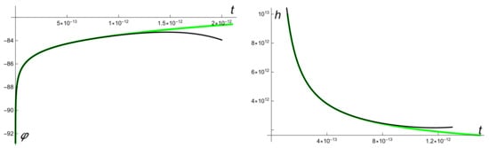
The results are exhibited in Figure 8 and Figure 9 for the same values of the parameters. In this case a solution with $N=60$ corresponds to $b=1.88634\times {10}^{26}$ while a solution with $N=70$ corresponds to $b=3.32729\times {10}^{29}$. The numerical solution with initial conditions ${\phi }_0=-100$, $h_0=h_{approx,m}^{(-)}({\phi }_0,b_{60})$ gives an amount of inflation $N_{num}\approx 59.9639$ and that with initial conditions ${\phi }_0=-300$, $h_0=h_{approx,m}^{(-)}({\phi }_0,b_{70})$ gives an amount of inflation $N_{num}\approx 69.9637$.

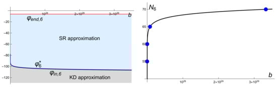
Figure 8. The left figure shows the lines ${\phi }_{in,6}\left(b\right)$ (black line), ${\phi }_6^{*}\left(b\right)$ (blue line), and ${\phi }_{end,6}$ (red line) for the solutions (30) of (31) with potential (11) for $\lambda =\frac{\sqrt{2}}{3}$, $\mu =\frac{\sqrt{3}}{4}$, $c_1=2\times {10}^{-10}$, $c_2=2.5\times {10}^{-10}$. Note that in this case the distance between the lines ${\phi }_{in,6}\left(b\right)$ and ${\phi }_6^{*}\left(b\right)$ is very small by comparison with the distance between the lines ${\phi }_6^{*}\left(b\right)$ and ${\phi }_{end,6}$. It also shows the regions in the $(b,\phi )$ plane corresponding to the KD approximation (gray region) and the SR approximation (blue region). The right figure shows the amount of the inflation $N_6\left(b\right)$. The blue dots indicate the values $N=55,60,65$, and 70.

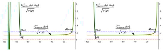
Figure 9. The green lines show the numerical solution ${\mathfrak{h}}^{(-)}\left(\phi \right)$ of (89) with initial conditions ${\phi }_0=-100$, ${\mathfrak{h}}_0=h_{approx,6}^{(-)}({\phi }_0,b_{60})/\sqrt{v\left({\phi }_0\right)}$ (left) and ${\phi }_0=-300$, ${\mathfrak{h}}_0=h_{approx,6}^{(-)}({\phi }_0,b_{70})/\sqrt{v\left({\phi }_0\right)}$ (right) for the model with potential (11) with $\lambda =\frac{\sqrt{2}}{3}$, $\mu =\frac{\sqrt{3}}{4}$, $c_1=2\times {10}^{-10}$, $c_2=2.5\times {10}^{-10}$. The black lines show the KD approximation $h_{approx,6}^{(-)}(\phi ,b_{60})/\sqrt{v\left(\phi \right)}$ (left) and $h_{approx,6}^{(-)}(\phi ,b_{70})/\sqrt{v\left(\phi \right)}$ (right) and the brown lines the SR approximation $h_{s,approx,6}^{(-)}\left(\phi \right)/\sqrt{v\left(\phi \right)}$. The regions between blue and red dotted lines are the inflation regions. The orange dotted lines correspond to the asymptotic behaviour of the separatrix solution ${\mathfrak{h}}_s\left(\phi \right)\sim {(1-{\lambda }^2)}^{-1/2}$ as $\phi \to -\infty$. The gray dots correspond (from left to right) to ${\phi }_{in,6}\left(b_{60}\right)$, ${\phi }_6^{*}\left(b_{60}\right)$ and ${\phi }_{end,6}$ (left figure) and ${\phi }_{in,6}\left(b_{70}\right)$, ${\phi }_6^{*}\left(b_{70}\right)$ and ${\phi }_{end,6}$ (right figure).

6. Conclusions

We have analysed the asymptotic properties of the solutions of a generalization of the Starobinski inflationary model determined by the potential (4). We have considered both the kinetic dominance and the slow roll periods within the Hamilton-Jacobi formalism, which provides a natural framework to determine generalized asymptotic expansions of the Hubble parameter as a function of the inflaton field.

We have found that the Hamilton-Jacobi Equation (17) in the KD period admits asymptotic expansion solutions as $\phi \to \infty$ which can be written as series in the variable $e^{-2\phi }$ with polynomial coefficients in the variables $e^{-2\lambda \phi }$ and $e^{-2\mu \phi }$. Moreover, if $\lambda <1$ we have proved that Equation (17) in the kinetic dominance period admits asymptotic expansions solutions as $\phi \to -\infty$, which can be written as series in $e^{2\phi }$ with have also polynomial coefficients in $e^{-2\lambda \phi }$ and $e^{-2\mu \phi }$. These asymptotic expansions depend on a free parameter b, and the polynomial coefficients can, in both cases, be recursively obtained (see Equation (58)), and indeed this recursion formula is easily programmed.

On the other hand, the solutions of (17) in the SR period behaves as separatrix solutions [19,30], when these separatrix solutions exist. Using the results of a previous work [34] we know that the inflation model (4) admits separatrix solution defined for $\phi >{\phi }_{min}$ for all $\lambda >0$ (we have denoted this separatrix solution by $h_s^{(+)}\left(\phi \right)$), and admits also a separatrix solution defined for $\phi <{\phi }_{min}$ provided that $0<\lambda <1$ (we have used here the notation $h_s^{(-)}\left(\phi \right)$).

It has been found that the separatrix solution $h_s^{(+)}\left(\phi \right)$ can be determined as an asymptotic expansion in powers of $e^{-2\lambda \phi }$ and $e^{-2\mu \phi }$ while the asymptotic expansion for the separatrix solution $h_s^{(-)}\left(\phi \right)$ can be written in powers of $e^{2\lambda \phi }$ with polynomial coefficients in $e^{-2\mu \phi }$. Again the coefficients in these expansions can be recursively determined and the recursive method is easily programmed.

All these expansions prove to be useful to obtain approximations to the solutions of (17) in the KD and SR periods. Thus given $m\in \mathbb{N}$ only a finite number of terms in the expansions as $\phi \to \infty$ (resp. $\phi \to -\infty$) are proportional to $e^{-c\phi }$ (resp. $e^{-c\phi }$) with $c\le m-1$.

In particular, we have considered the model for the value of the parameter ${\mathrm{\Lambda }}_3$ in (4) corresponding to $V\left({\varphi }_{min}\right)=0$. The corresponding expansions have been applied to determine the values of the inflaton field when the period of inflation starts ${\phi }_{in}$ and ends ${\phi }_{end}$, as well as to compute the amount of inflation as a function of the free parameter b in the KD period. Thus, this function can be used to select the appropriate value of the free parameter, and consequently the appropriate initial conditions, for a solution with a previously fixed amount of inflation.

Finally, we mention that many of the results in this work could be easily formulated for models with an exponentially potential well

$$V\left(\varphi \right)={\mathrm{\Lambda }}_1{e}^{\lambda \varphi }+{\mathrm{\Lambda }}_2{e}^{-\mu \varphi }-{\mathrm{\Lambda }}_3,$$

with $0<\lambda ,\mu <1$ and ${\mathrm{\Lambda }}_1,{\mathrm{\Lambda }}_2,{\mathrm{\Lambda }}_3>0$ (see for instance the models consider in [41]).

References

- Starobinsky, A. A new type of isotropic cosmological models without singularity. Phys. Lett. B 1980, 91, 99. [Google Scholar] [CrossRef]
- Guth, A.H. Inflationary universe: A possible solution to the horizon and flatness problems. Phys. Rev. D 1981, 23, 347–356. [Google Scholar] [CrossRef] [Green Version]
- Linde, A.D. A new inflationary universe scenario: A possible solution of the horizon, flatness, homogeneity, isotropy and primordial monopole problems. Phys. Lett. B 1982, 108, 389–393. [Google Scholar] [CrossRef]
- Linde, A.D. Initial conditions for inflation. Phys. Lett. B 1985, 162, 281–286. [Google Scholar] [CrossRef]
- Mukhanov, V. Physical Foundations of Cosmology; Cambridge University Press: Cambridge, UK, 2005. [Google Scholar]
- Baumann, D. TASI Lectures on Inflation. TASI Lectures on Inflation. arXiv 2009, arXiv:0907.5424. [Google Scholar]
- Starobinskii, A. The perturbation spectrum evolving from a nonsingular initially de-Sitter cosmology and the microwave background anisotropy. Sov. Astron. Lett. 1983, 9, 302–304. [Google Scholar]
- Linde, A.D. Chaotic inflation. Phys. Lett. B 1983, 129, 177–181. [Google Scholar] [CrossRef]
- Kallosh, R.; Linde, A. Universality class in conformal inflation. J. Cosmol. Astropart. Phys. 2013, 2013, 002. [Google Scholar] [CrossRef] [Green Version]
- Akrami, Y.; Kallosh, R.; Linde, A.; Vardanyan, V. Dark energy, α-attractors, and large-scale structure surveys. J. Cosmol. Astropart. Phys. 2018, 2018, 041. [Google Scholar] [CrossRef] [Green Version]
- Liddle, A.R. Power-law inflation with exponential potentials. Phys. Lett. B 1989, 220, 502–508. [Google Scholar] [CrossRef]
- Fomin, I.; Chervon, S. Exact and slow-roll solutions for exponential power-Law inflation connected with modified gravity and observational constraints. Universe 2020, 6, 199. [Google Scholar] [CrossRef]
- Lasenby, A.; Doran, C. Closed universes, de Sitter space, and inflation. Phys. Rev. D 2005, 71, 063502. [Google Scholar] [CrossRef] [Green Version]
- Handley, W.; Brechet, S.; Lasenby, A.; Hobson, M.P. Kinetic initial conditions for inflation. Phys. Rev. D 2014, 89, 063505. [Google Scholar] [CrossRef] [Green Version]
- Handley, W.; Lasenby, A.; Hobson, M. Kinetically dominated curved universes: Logolinear series expansions. Phys. Rev. D 2019, 99, 123512. [Google Scholar] [CrossRef] [Green Version]
- Destri, C.; de Vega, H.; Sanchez, N.G. The pre-inflationary and inflationary fast-roll eras and their signatures in the low CMB multipoles. Phys. Rev. D 2010, 81, 063520. [Google Scholar] [CrossRef] [Green Version]
- Steinhardt, P.J.; Turner, M.S. Prescription for successful new inflation. Phys. Rev. D 1984, 29, 2162. [Google Scholar] [CrossRef] [Green Version]
- Stewart, E.D.; Lyth, D.H. A more accurate analytic calculation of the spectrum of cosmological perturbations produced during inflation. Phys. Lett. B 1993, 302, 171–175. [Google Scholar] [CrossRef] [Green Version]
- Liddle, A.R.; Parsons, P.; Barrow, J.D. Formalizing the slow-roll approximation in inflation. Phys. Rev. D 1994, 50, 7222. [Google Scholar] [CrossRef]
- Lidsey, J.E.; Liddle, A.R.; Kolb, E.W.; Copeland, E.J.; Barreiro, T.; Abney, M. Reconstructing the inflaton potential—An overview. Rev. Mod. Phys. 1997, 69, 373. [Google Scholar] [CrossRef]
- Bassett, B.A.; Tsujikawa, S.; Wands, D. Inflation dynamics and reheating. Rev. Mod. Phys. 2006, 78, 537–589. [Google Scholar] [CrossRef] [Green Version]
- Linde, A. Inflationary Cosmology. In Inflationary Cosmology; Lecture Notes in Physics; Springer: Berlin, Germany, 2008; Volume 738, pp. 1–54. [Google Scholar]
- Weinberg, S. Cosmology; Oxford University Press: Oxford, UK, 2008. [Google Scholar]
- Boyanovsky, D.; Destri, C.; de Vega, H.; Sanchez, N. The Effective Theory of Inflation in the Standard Model of the Universe and the CMB+LSS data analysis. Int. J. Mod. Phys. A 2009, 24, 3669–3864. [Google Scholar] [CrossRef] [Green Version]
- Haddadin, W.I.J.; Handley, W.J. Rapid numerical solutions for the Mukhanov-Sazaki equation. arXiv 2018, arXiv:1809.11095. [Google Scholar]
- Hergt, L.; Handley, W.; Hobson, M.; Lasenby, A. Constraining the kinetically dominated universe. Phys. Rev. D 2019, 100, 023501. [Google Scholar] [CrossRef] [Green Version]
- Hergt, L.; Handley, W.; Hobson, M.; Lasenby, A. Case for kinetically dominated initial conditions for inflation. Phys. Rev. D 2019, 100, 023502. [Google Scholar] [CrossRef] [Green Version]
- Hille, E.I. Ordinary Differential Equations in the Complex Domain; Courier Corporation: New York, NY, USA, 1997. [Google Scholar]
- Medina, E.; Alonso, L.M. Kinetic dominance and psi series in the Hamilton-Jacobi formulation of inflaton models. Phys. Rev. D 2020, 102, 103517. [Google Scholar] [CrossRef]
- Belinskii, V.A.; Grishchuk, L.P.; Zel’dovich, Y.B.; Khalatnikov, I.M. Inflationary stages in cosmological models with a scalar field. Sov. Phys. JETP 1985, 62, 195. [Google Scholar] [CrossRef]
- Álvarez, G.; Martínez Alonso, L.; Medina, E.; Vázquez, J.L. Separatrices in the Hamilton–Jacobi formalism of inflaton models. J. Math. Phys. 2020, 61, 043501. [Google Scholar] [CrossRef] [Green Version]
- Albrecht, A.; Steinhardt, P.J.; Turner, M.S.; Wilczek, F. Reheating an Inflationary Universe. Phys. Rev. Lett. 1982, 48, 1437. [Google Scholar] [CrossRef]
- Shtanov, Y.; Traschen, J.; Brandenberg, R. Universe reheating after inflation. Phys. Rev. D 1995, 51, 5438. [Google Scholar] [CrossRef] [PubMed] [Green Version]
- Álvarez, G.; Martínez Alonso, L.; Medina, E. Generalised asymptotic solutions for the inflaton in the oscillatory phase of reheating. Universe 2021, 7, 390. [Google Scholar] [CrossRef]
- Salopek, D.; Bond, J. Nonlinear evolution of long-wavelength metric fluctuations in inflationary models. Phys. Rev. D 1990, 42, 3936. [Google Scholar] [CrossRef] [PubMed]
- Lyth, D.H.; Liddle, A.R. The Primordial Density Perturbation: Cosmology, Inflation and the Origin of Structure; Cambridge University Press: Cambridge, UK, 2009. [Google Scholar]
- Baumann, D. Cosmology, Part III Mathematical Tripos; University Lecture Notes: Cambridge, UK, 2012. [Google Scholar]
- Dodelson, S. Modern Cosmology; Academic Press: San Diego, CA, USA, 2003. [Google Scholar]
- Martin, J. The Theory of Inflation. 200th Course of Enrico Fermi School of Physics: Gravitational Waves and Cosmology. arXiv 2018, arXiv:1807.11075. [Google Scholar]
- John, F. Partial Differential Equations; Springer: New York, NY, USA, 1982. [Google Scholar]
- Foster, S. Scalar field cosmological models with hard potential walls. arXiv 1998, arXiv:gr-qc/9806113. [Google Scholar]
- Bell, E.T. Exponential polynomials. Ann. Math. 1934, 258–277. [Google Scholar] [CrossRef]
Publisher’s Note: MDPI stays neutral with regard to jurisdictional claims in published maps and institutional affiliations. |
© 2021 by the authors. Licensee MDPI, Basel, Switzerland. This article is an open access article distributed under the terms and conditions of the Creative Commons Attribution (CC BY) license (https://creativecommons.org/licenses/by/4.0/).