Abstract
In this work, we study the relativistic quantum motion of an electron in the presence of external magnetic fields in the spinning cosmic string spacetime. The approach takes into account the terms that explicitly depend on the particle spin in the Dirac equation. The inclusion of the spin element in the solution of the problem reveals that the energy spectrum is modified. We determine the energies and wave functions using the self-adjoint extension method. The technique used is based on boundary conditions allowed by the system. We investigate the profiles of the energies found. We also investigate some particular cases for the energies and compare them with the results in the literature.
Data Set License: license under which the data set is made available (CC0, CC-BY, CC-BY-SA, CC-BY-NC, etc.)
1. Introduction
The concept of singularity is an essential one in several branches of Mathematics and Physics. In Mathematics, it appears, for instance, in the study of differential equations, geometry, and topology [1]. In Physics, it can show up in the mathematical machinery describing phenomena of interest, or it can be a singularity intrinsically involved in the physical system [2]. For example, the spacetime itself can contain singularities due to the presence of black holes [3] or topological defects of cosmological origin [4].
It is common sense that the physical properties of a given system depend on the form of spacetime where it is inserted. The presence of curvature or torsion, for instance, can affect such properties. Even the light propagation can be influenced under such conditions [5], which can be understood by the notion of geodesics [6]. A particularly relevant case involving curved spacetimes and singularities occur when a topological defect shows up in producing a singularity associated with a conical space [7]. A wide range of works has dedicated attention to the issue of describing how physical quantities of interest are affected by the influence of a conical spacetime. It happens because the conical geometry can take place in many different contexts. Examples of this can be found in the study of the propagation of optical beams [8] and in research on the existence of graphite nanocones and microcones [9]. In addition, oxide graphene membranes with conical channels can be used for ultrafast water transport [10]. In condensed matter physics, a topological defect known as disclination is associated with the conical geometry. It appears, for example, in studying Liquid Crystals [11,12]. It is possible to understand the formation of a disclination from a flat material by employing the process of Volterra [13]. In this process, a circular sector of material can be inserted into the sample or removed from it, and thus constructing a conical surface.
While a disclination is related to materials, there is an analog of such defect that occurs in spacetime: the cosmic string. The latter consists of a linear defect, whose spacetime around it is globally conical. Concerning the origin of these defects, it is believed that they were generated due to phase transitions in the early Universe [14]. They are theoretically predicted in many models in particle physics and are expected to create gravitational waves. In the case that this hypothesis is confirmed, it could provide us an extraordinary tool to study the history of the Universe [15]. A discussion about the search for signatures of cosmic strings from an observational point of view can be encountered in [16]. In cylindrical coordinates , the line element of a cosmic string is written as
In this expression, , , and . The parameter tells us about the presence of a conical geometry, providing an idea of how much the flat spacetime was affected by the presence of the topological defect. It is associated with the , the mass per unit length of the cosmic string. More explicitly, and it is defined in the interval . Thus, the case refers to the flat Minkowski spacetime in cylindrical coordinates [17]. This metric also can be imagined as a spacetime containing a conical singularity located at the origin, [18]. It can be expressed in terms of the unique non-vanishing component of the curvature tensor
where indicates the two-dimensional Dirac delta function. The line element describing a disclination is identical to that of the Equation (1), but this time we can think the parameter as the angular deficit which comes from the Volterra process. Since we made this comparison between disclinations and cosmic strings, at this point, it is worth noting that it is possible to employ the framework of Riemann–Cartan geometry to model defects in solids, as pointed by Katanaev and Volovich [19]. A curious connection between condensed matter systems and general relativity was opened [20].
Both disclinations and cosmic strings have been considered as a background for studying several physical systems. The study of quantum systems is especially a stimulating issue because uncommon characteristics in such systems can take place when compared to the classical scenario. For example, the gravitational field near cosmic strings can produce effects on quantum fields like vacuum polarisation and particle production [21]. The influence of this background was also considered in the analysis of electron–positron pair production [22], in the Casimir effect [23], and in the relativistic hydrogen atom model [24]. The appearance of geometric phases in the conical geometry is also a subject of study in this context. Some realizations can be found in the study of graphene with disclinations [25] and in the analysis of the two-level atom model in the spacetime of a cosmic string [26]. More recently, the notion of quantum entanglement in the spacetime of a cosmic string also has been analyzed [27,28].
Besides these aspects involving quantum systems in the conical spacetime background, another important question in this context is related to the presence of electromagnetic interactions. Contributions in this direction appear in the study of Landau levels for a non-relativistic electron in the presence of disclinations [29] and in the solution of the two-dimensional electron gas problem [30]. Other interesting works were also developed in this context as, for example, the determination of the low-energy spectrum of graphene with a disclination [31], the study of the relativistic quantum motion of spin-0 and spin-1/2 particles in the spacetime of a cosmic string [32], and also problems including the Aharonov–Bohm potential [33,34].
Up to now, we have mentioned examples dealing with the quantum description of a system in the presence of disclinations and cosmic strings. In most of these works, the main objective is to show that the topological defect affects the physical properties of the system, such as the energy levels of wave functions. These effects are observed even in the region. However, since the region presents a singularity in conical spacetime, the quantum mechanical description for this problem requires a more appropriate mathematical formulation of quantum mechanics. More explicitly, if we are interested in also describing the behavior of a quantum system at , we need to employ the self-adjoint approach [35,36,37,38,39,40,41,42]. It is necessary since the quantum operators which describe the physical observables are not well defined in such region: such operators are not self-adjoint, as it should be. For instance, if we are interested in obtaining the energy spectrum of a given system, we will need to proceed by making the self-adjoint extension of the Hamiltonian [43]. At this point, it is worth mentioning that, besides the self-adjoint extension method, there is another way to deal with singularities in quantum mechanics. More specifically, it is also possible to employ the framework of the Weyl–Heisenberg integral quantization [44]. While the self-adjoint extension method deals with singularities by starting with a quantum mechanical description, the Weyl–Heisenberg quantization provides a way to quantize a classical system. In that quantization procedure, the singularities might be removed. Further details and information on the Weyl–Heisenberg method can be found in the literature [45,46,47,48].
Similar to the electromagnetic interactions, the investigation of noninertial effects in the context of the conical geometry has attracted attention, and curious theoretical predictions have been achieved. These characteristics are found, for example, in the study of the relativistic quantum motion of scalar bosons [49], in the description of the two-dimensional electron gas model [50], in the relativistic Landau quantization [51], and problems involving the Dirac oscillator [52,53,54].
Although there is a rich literature dealing with several quantum systems in the spinning cosmic string spacetime, there is a lack of works related to the application of the self-adjoint approach considering this background. Motivated by this fact, in this paper, we study the problem of a spin-1/2 particle in such a scenario. Having in mind the importance of the electromagnetic interactions, we also include the presence of a uniform magnetic field and the Aharonov–Bohm effect. In Section 2, we present the algebraic ingredients necessary for obtaining the Dirac equation in the spinning cosmic string background. We define the field configuration involved, and using appropriate eigenfunctions and spinor decomposition, we find the radial equation of motion of the model. In Section 3, we review some basic properties and concepts of the self-adjoint extension method and write the boundary condition to be employed in solving the equation of eigenvalues. In Section 4, we apply the boundary condition to the problem and find a relation that allows us to find the energies of the particle. We study the spectrum in detail and compare it with results in the literature. We finish this section by analyzing some particular cases for the model studied. We make our concluding remarks in Section 5.
2. Dirac Equation in the Spinning Cosmic String Spacetime
In this section, we present the physical environment necessary to write the Dirac equation in curved spacetime. The first step is to obtain Dirac’s Hamiltonian in the spinning cosmic string background. We already wrote the line element for a static cosmic string spacetime. Now, we shall introduce the presence of rotation. Since we are dealing with cylindrical symmetry, the rotation is related to the coordinates t and . Explicitly, the metric tensor that describes this spacetime is a generalization of the metric (1), which is written as [55]
where a is the parameter that describes the rotation, which depends on the angular momentum J of the cosmic string through the relation . A crucial difference between (1) and (3) is that the latter allows the existence of closed timelike curves when . In this manuscript, we are not interested in considering such curves.
To study the relativistic quantum motion of an electron interacting with external magnetic fields in the metric spacetime (3), we need to write the generic Dirac equation in a curved space, given by
where M represents the mass of the particle, is the four-potential of the electromagnetic field, are the Dirac matrices in the curved space, and is the covariant derivative for fermion fields, which is defined by
with being the spin affine connection, which can be calculated through the relation
where are the Christoffel symbols of the second kind and is the tetrad field to be defined later. The matrices are related to the usual Dirac matrices (in the flat spacetime) through the expression
with being the tetrad field, which obeys the relations
In the expressions above and along the manuscript, are the indices which indicate the local reference frame while indicate the curved spacetime. More precisely, we use the Greek letters to represent the tensor indices while the Latin letters are denoting Minkowski indices. The matrices are given by
where indicates the standard Pauli matrices. The matrices (7) satisfy the following property:
We use the tetrad basis and its inverse defined as [55]
In the absence of rotation, we recover the tetrad basis used in Refs. [56,57,58]. For the tetrad field above, the affine connection is found to be
with
where
Note that, for the particular choice of the tetrad (13), the affine connection is identically null when (flat space). In the tetrad basis (13), the matrices (7) can be written explicitly as
We can also define the matrices1, which can be written in terms of Pauli’s matrices as
where are the Pauli matrices in cylindrical coordinates written on the tetrad basis . Such matrices are explicitly written as
We already have the geometric tools we need to describe the quantum motion of the electron in the spinning cosmic string background. Now, we need to define the magnetic interaction. Since the system exhibits symmetry of translation with respect to z direction, we can assume , which leads just to a plane motion [42,59,60,61]. We consider the particle in the presence of a potential vector superposition (in the Coulomb gauge) given by
where is given in terms of the potential that gives rise to the uniform magnetic field plus the potential that describes the Aharonov–Bohm effect as
with B being the magnitude of the uniform magnetic field, , where is the magnetic flux and is the quantized magnetic flux related to the Aharonov–Bohm potential. The magnetic fields associated with the Equation (25) are found to be
where corresponds to the uniform magnetic field and to the Aharonov–Bohm flux tube. Note that the magnetic field is given in terms of the function, which is a short-range potential. We are interested in analyzing the electron motion including the region, in such a way that the field cannot be neglected in the approach. In other words, we need to solve the Dirac equation taking into account irregular solutions at the origin. From this point, we will be interested in obtaining the radial equation for the problem. After this step, we will discuss the inclusion of the function in the equation of motion in more detail. Assuming the time-dependence of the eigenfunctions in the form and decomposing the spinor
we find the following matrix equation:
As the potential vector only has the component (Equation (23)), Equation (28) can be written as
which can still be written as
Equations (31) and (32) allow us to obtain a second order equation for both and with the requirement that . We chose to study the equation for . By isolating in Equation (32) and replacing in Equation (31), we obtain
where
is the Dirac hamiltonian and
Making use of the underlying rotational symmetry expressed by the fact that , where
is the total angular momentum operator in the z-direction, we decompose the Hilbert space with respect to the angular momentum , where and , with denoting the unit sphere in . Thus, it is possible to express the eigenfunctions of the two-dimensional Hamiltonian in terms of the eigenfunctions of as
where is the angular momentum quantum number. Substituting (37) in Equation (33) together with Equations (25) and (26), we obtain the following equations:
with
and
where
represent the effective angular momenta and
where , with being the cyclotron frequency. We can notice the presence of the function potential in Equations (39) and (40). The operator is a relativistic generalization of the Landau quantization in the presence of the spin-1/2 Aharonov–Bohm effect for the case where the particle is subject to both topological and noninertial effects. As pointed out by Hagen [62], the Aharonov–Bohm effect possesses an exact equivalence with the Aharonov–Casher effect for spin-1/2 particles. Such equivalence is guaranteed just when we consider the spin of the particle in the approach. When we wish to study these models considering the spin of the particle, the following requirement arises: the term involving the function in the operator cannot be neglected. It is known in the literature that the presence of such interaction guarantees the existence of bound states in Aharonov–Bohm-type systems [60,61,63,64,65,66]. Then, we shall solve Equation (38) for bound states using the self-adjoint extension technique [35].
3. Self-Adjoint Extension
In this section, we study the dynamics of the system in all space, including the region. We consider the problem of bound states, by employing the self-adjoint extension method in the treatment. As is well known, if the Hamiltonian has a point-like singularity, as is the case of the Hamiltonian in Equation (38), we shall verify that it is self-adjoint in the region of interest. Let us consider two arbitrary operators and . If the domain of contains the domain of , or more formally, , and in the domain of the operators are equals, then we can state that the operator is an extension of the the operator . In this configuration, if the domain of the operator is dense, then for each vector in this domain, there is a sequence , so that we have . Hence, the domain of its adjoint , is the set of all vectors for which there is a vector satisfying the relation for all vectors . From this relation, we define . We can also establish that an operator with dense domain is symmetric if for every and in its domain. In this case, can be defined as for all , and is said to be an extension of . If , then is called self-adjoint operator or Hermitian operator. It is important to note that a symmetric operator can fail to be a self-adjoint operator. For the operator to be a self-adjoint operator, it has to be symmetric, , and the domains of the operator and its adjoint have to be equal as well, i.e., .
According to the above definitions, the operator , with domain is said to be self-adjoint if and only if , , with being the adjoint of operator and, moreover, it has to be symmetrical. In addition, for smooth functions, , with , we should have . In this case, it is possible to interpret as a self-adjoint extension of [64,67,68]. The self-adjoint extension method consists in extending the domain of in order to match . It is known that the operator is essentially self-adjoint for , while, for , it admits a one-parameter family of self-adjoint extensions [35], said , where is the self-adjoint extension parameter of the problem. To characterize this family, we shall use the approach developed in Refs. [69,70], which is based on the boundary conditions at the origin. All the self-adjoint extensions of are parametrized by the boundary condition at the origin
with
where is the self-adjoint extension parameter. Physically, it is known that the quantity can be interpreted as the scattering length of (More details on this issue are given in Ref. [70]). For , the boundary condition represents the Friedrichs extension of . In the case of Equation (38), it means that we are studying the Dirac equation without taking into account terms that explicitly depend on the spin of the particle, with regular wave functions at the origin (). This situation is analogous to imposing the Dirichlet boundary condition on the wave function , which allows us to recover the original results of Ref. [71]. On the other hand, if we consider , the operator characterizes a point interaction at region. In this case, the boundary condition permits a singularity in the wave functions at this point [72] (we show this in the next section). For , we have the free Hamiltonian (without the function). For this last case, the boundary condition reveals that only regular wave functions at the origin are considered. According to the theory of self-adjoint extensions, we can not impose any boundary condition without discovering which boundary conditions are allowed to Equation (38) [35]. For the model in question, the operator is one that satisfies the boundary condition (46). Another question that needs to be clarified here is related to the choice of the parameter . Since we are dealing with a non-confined relativistic quantum system, we must ensure that is finite in the range (), which is a necessary and sufficient condition for it to be square-integrable and also to ensure the existence of bound state solutions.
4. The Energy Spectrum
In this section, we solve Equation (38) in the region to determine the energies of the particle in the spinning cosmic string spacetime. By using the variable change , Equation (46) can be written as
Due to the boundary condition in Equation (46), we shall take into account regular and irregular solutions for Equation (49). Studying the asymptotic limits of Equation (49), we obtain the following regular (+) (irregular (−)) solution:
Equation (51) is a confluent hypergeometric equation type
The general solution of Equation (51) is
where denotes the Kummer function (or confluent hypergeometric function of the first kind ), while represents the confluent hypergeometric function of the second kind [73], and and are constants of normalization. Using the property
the solution (53) can be fully expressed in terms of the Kummer function. Consequently, the solution (50) assumes the form
where and are, respectively, the coefficients of the regular and irregular solutions at the origin, and
Now, we will apply the contour condition (46) to the problem. We need to use the solution (55) together with the series expansion until first order in y for the function , given by
After some intermediate steps, we obtain the following relation between the coefficients and :
By studying the , we verify that it diverges if . From this condition, we can establish that must be zero if and only the regular solution contributes to . As mentioned above, if , we have only the situation when the operator is not self-adjoint. In this case, a contribution of the irregular solution to at the origin [61,74,75,76,77,78,79] turns up. In other words, the contribution of the irregular solution for the system wave function stems from the fact that the operator is not self-adjoint.
For be a bound state wave function, it must vanish at large values of r. In addition, it must be a normalizable wave function. These conditions allow us to obtain another relationship involving the constants and . Then, using the asymptotic representation of the confluent hypergeometric function for large argument,
we obtain the relation
where
Equation (62) can be simplified by studying the behavior from X and Y for . The resulting equation is
Now, let’s return to Equation (60) and consider the condition . It provides
We can see that Equation (67) determines, implicitly, the energies of the particle for different values of . For the present system, we investigate two values, which are related to the boundary conditions at the origin and at infinity, respectively. For , when the function is absent, only the regular solution contributes to the bound state wave function. For , only the irregular solution contributes to the bound state wave function. For all other values of , both regular and irregular solutions contribute to the bound state wave function. The energies for the two cases above are accessed by studying the poles of the function through the relations [58,80]
with . Note that, in Equations (68) and (69), the quantity (see Equations (42) and (43)) is given in terms of the energy . Thus, to find an expression for the energy eigenvalues, we must consider and , respectively, and then solve these expressions for . We obtain the following energies:
- (i)
- For the case :
- (ii)
- For the case :with
The above energies present some curious characteristics. When we compare the energies and , we see that they are the same. The same occurs when we compare , and . We also notice that and are independent of the parameters m, , and a while and are given in terms of all the physical parameters involved in the model. The energies of the regular solution (70) and (71) can be compared with the energies (47) and (50) of Ref. [55], respectively, for the particular case when the cyclotron frequency plays the role of the Dirac oscillator frequency. We make some energy sketches as a function of some parameters of the system. In all the figures, we consider . Because of the dependence on all the parameters of the model and the similarity with the other energies, we prefer to analyze only the energy (71). We use solid and dashed-dotted lines to represent the energy of the particle and dashed and dotted lines to the antiparticle. In Figure 1, we investigate the profile of as a function of . When , and , the spectrum is located in the energy range . In addition, we also note that the energies increase when is increased or equivalently, when the magnetic field B is increased (Figure 1a). This is verified for (blue color), (red color) and (green color) for and (both identified in the figures). On the other hand, when we change the curvature and the flux to and and keeping the same parameter a, the spectrum assumes the profile of Figure 1b (for and ). In this case, we can see that the energies increase when n increases and m decreases. In both cases, we can also clearly see that the spectrum is not symmetrical about . In fact, when in Equations (71), (73), (74) and (76), the symmetry is recovered.
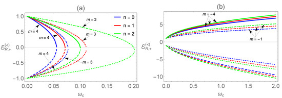
Figure 1.
Sketch of the energy levels (Equation (71)) as a function of . In (a), , , . In (b), , , .
When we investigate the profile of as a function of , we verify that the spectrum is negative (Figure 2). In particular, when , and for and , we can see that the energies increase when is increased and m is decreased (Figure 2a). Furthermore, energies are only allowed for . In Figure 2b, we show the profile for , and for and . For this configuration, we see that increases when n increases. However, when the rotation is lower, ranges of emerge in which the energy is forbidden.

Figure 2.
Sketch of the energy levels (Equation (71)) as a function of . In (a), , and . In (b), , and .
The sketch of as a function of rotation is depicted in Figure 3. Considering , and , we see that the increases when n is increased and m is decreased. For simplicity’s sake, we consider and (Figure 3a). On the other hand, when we consider the parameters , and for and , we see that the energy states of the particle (solid and dashed-dotted lines) are closer to each other while those of the antiparticle (dashed and dotted line) are more separated when approaches 1 (Figure 3b).
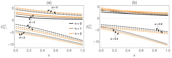
Figure 3.
Sketch of the energy levels (Equation (71)) as a function of a. In (a), we use , and for and . In (b), we use , and for and .
The profile of as a function of is displayed in Figure 4 considering two settings. In the first one, we use , and for and (Figure 4a). As in the other cases analyzed above, we also observe an increment in the spectrum when n increases. We also verify that the energy states with are closer to each other while the states with are more separate. In addition, a flux range appears where energy is forbidden. In the second situation, we use , , and keeping the same values of m. In this case, we observe that increases as well as the flux range where the energy is forbidden.
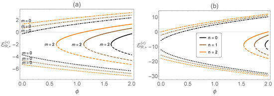
Figure 4.
Sketch of the energy levels (Equation (71)) as a function of . In (a), , and and, In (b), , and .
According to the discussion presented in Section 3, we can state that, for or when the function is absent, only the regular solution contributes to the bound state wave function. In this case, the energy is given by Equation (82). Differently, when the solution is singular at the origin, the corresponding energy is given by Equation (83). Energies (82) and (83) are equivalent to the energies (46) of Ref. [58]. Moreover, we also see that they are symmetrical around in both regular and irregular cases. As a final investigation, making (flat space) and (no magnetic flux), we no longer have any curvature effect and the term involving the interaction is absent. In this case, only regular solutions are considered and the Equation (82) implies the usual Landau relativistic quantization [81]
which is an important result that has several important applications in many branches of physics.
5. Conclusions
In the present manuscript, we have addressed the problem of the relativistic quantum motion of an electron in the spinning cosmic string background in the presence of a uniform magnetic field and the Aharonov–Bohm potential. The new ingredients in the study of this model are the inclusion of the spin degree of freedom and the solution of the quantum motion equation by using the self-adjoint extension method. We have written the Dirac equation describing the model (Equation (28)) and derived the second-order equation for the upper component of the spinor (Equation (33)).
We have used an appropriate ansatz (Equation (37)) and obtained the radial equation corresponding to the bispinor (Equation (38)). The radial equation includes the function which arises due to the interaction between the magnetic field and the particle spin at . The inclusion of spin effects in the solution of the problem is also the reason why the particle can access the region in the model studied. We have shown that this process requires that irregular solutions at the shall be considered in the treatment of the problem. Having this in mind, we have employed the self-adjoint extension method based on boundary conditions at the origin (Equation (46)). The boundary condition revealed to us that the operator is self-adjoint only if . Outside this range, i.e., for , is not self-adjoint. The boundary condition (46) and the analysis of the asymptotic behavior of the solution (Equation (55)) both allowed us to obtain a relation between the constants and . As a result, we obtained a relation that allowed us to find the energies of the particle in terms of the self-adjoint extension parameter, . We have considered two values for , which are related to the boundary conditions at the and at the infinity, namely and . For each of these conditions, we find the corresponding energy for the particle.
The presence of non-inertial effects shows us that the energy spectrum of the particle is given by eight equations (Equations (70)–(77)). However, we have identified by direct comparison that the energies , , and are equals. We have found that the energies and depend only on M, n and while the energies and depend on all physical parameters of the model. We have argued that the energies and are symmetric about zero energy while and present this characteristic only in the absence of rotation. Because of the condition , few energy states of the particle are inside of this interval. For the model studied, only the states with and belong to this range. For this reason, we analyze graphically only the energy . We exhibited the profile of as a function of , , a and . In all cases investigated, we verified that both the curvature and rotation modify the energy levels of the particle. To finish the work, we studied some particular cases to show that the model studied is consistent with other results in the literature.
Author Contributions
E.O.S.: Conceptualization, methodology, software, supervision, writing—original draft preparation, writing—review and editing, project administration; M.M.C.: Writing—original draft preparation, formal analysis, investigation. All authors have read and agreed to the published version of the manuscript.
Funding
This work was partially supported by the Brazilian agencies CAPES, CNPq and FAPEMA. E.O.S. acknowledges CNPq Grants 427214/2016-5 and 307203/2019-0, and FAPEMA Grants 01852/14 and 01202/16. This study was financed in part by the Coordenação de Aperfeiçoamento de Pessoal de Nível Superior-Brasil (CAPES)–Finance Code 001. M.M.C. acknowledges CAPES Grant 88887.358036/2019-00.
Acknowledgments
We would like to thank R.C. (Universidade Federal do Maranhão, MA, Brazil) for his remarks and comments.
Conflicts of Interest
The authors declare no conflict of interest.
References
- Brasselet, J.P. Singularities in Geometry and Topology: Proceedings of the Trieste Singularity Summer School and Workshop, ICTP, Trieste, Italy, 15 August–3 September 2005; World Scientific: Singapore, 2007. [Google Scholar]
- Konkowski, D.A.; Helliwell, T.M. Understanding singularities—Classical and quantum. Int. J. Mod. Phys. A 2016, 31, 1641007. [Google Scholar] [CrossRef]
- D’Inverno, R. Introducing Einstein’s Relativity; Clarendon Press: Oxford, UK, 1992. [Google Scholar]
- Bäuerle, C.; Bunkov, Y.M.; Fisher, S.; Godfrin, H.; Pickett, G. Laboratory simulation of cosmic string formation in the early Universe using superfluid 3 He. Nature 1996, 382, 332–334. [Google Scholar] [CrossRef]
- Schultheiss, V.H.; Batz, S.; Szameit, A.; Dreisow, F.; Nolte, S.; Tünnermann, A.; Longhi, S.; Peschel, U. Optics in Curved Space. Phys. Rev. Lett. 2010, 105, 143901. [Google Scholar] [CrossRef] [PubMed]
- Radożycki, T. Geometrical optics and geodesics in thin layers. Phys. Rev. A 2018, 98, 063802. [Google Scholar] [CrossRef]
- Vilenkin, A.; Shellard, E.P. Cosmic Strings and Other Topological Defects; Cambridge University Press: Cambridge, UK, 2000. [Google Scholar]
- Zhang, Y.L.; Dong, X.Z.; Zheng, M.L.; Zhao, Z.S.; Duan, X.M. Steering electromagnetic beams with conical curvature singularities. Opt. Lett. 2015, 40, 4783–4786. [Google Scholar] [CrossRef]
- Gogotsi, Y.; Dimovski, S.; Libera, J. Conical crystals of graphite. Carbon 2002, 40, 2263–2267. [Google Scholar] [CrossRef]
- Ma, Y.; Su, Y.; He, M.; Shi, B.; Zhang, R.; Shen, J.; Jiang, Z. Graphene oxide membranes with conical nanochannels for ultrafast water transport. ACS Appl. Mater. Interfaces 2018, 10, 37489–37497. [Google Scholar] [CrossRef] [PubMed]
- Denniston, C. Disclination dynamics in nematic liquid crystals. Phys. Rev. B 1996, 54, 6272–6275. [Google Scholar] [CrossRef]
- Kleman, M. Defects in liquid crystals. Rep. Prog. Phys. 1989, 52, 555–654. [Google Scholar] [CrossRef]
- Puntigam, R.A.; Soleng, H.H. Volterra distortions, spinning strings, and cosmic defects. Class. Quantum Gravity 1997, 14, 1129. [Google Scholar] [CrossRef]
- Hindmarsh, M.B.; Kibble, T.W.B. Cosmic strings. Rep. Prog. Phys. 1995, 58, 477–562. [Google Scholar] [CrossRef]
- Cui, Y.; Lewicki, M.; Morrissey, D.E.; Wells, J.D. Cosmic archaeology with gravitational waves from cosmic strings. Phys. Rev. D 2018, 97, 123505. [Google Scholar] [CrossRef]
- Brandenberger, R.H. Searching for Cosmic Strings in New Observational Windows. Nucl. Phys. B Proc. Suppl. 2014, 246–247, 45–57. [Google Scholar] [CrossRef]
- Svaiter, B.F.; Svaiter, N.F. Quantum processes: Stimulated and spontaneous emission near cosmic strings. Class. Quantum Gravity 1994, 11, 347–358. [Google Scholar] [CrossRef]
- Sokoloff, D.D.; Starobinskii, A.A. On the structure of curvature tensor on conical singularities. Dokl. Akad. Nauk 1977, 234, 1043–1046. [Google Scholar]
- Katanaev, M.O.; Volovich, I.V. Theory of defects in solids and three-dimensional gravity. Ann. Phys. 1992, 216, 1–28. [Google Scholar] [CrossRef]
- Moraes, F. Condensed Matter Physics as a laboratory for gravitation and Cosmology. Braz. J. Phys. 2000, 30, 304–308. [Google Scholar] [CrossRef]
- Davies, P.C.W.; Sahni, V. Quantum gravitational effects near cosmic strings. Class. Quantum Gravity 1988, 5, 1. [Google Scholar] [CrossRef]
- Skarzhinsky, V.D.; Harari, D.D.; Jasper, U. Quantum electrodynamics in the gravitational field of a cosmic string. Phys. Rev. D 1994, 49, 755–762. [Google Scholar] [CrossRef]
- Moraes, F. Casimir effect around disclinations. Phys. Lett. A 1995, 204, 399–404. [Google Scholar] [CrossRef]
- Marques, G.D.; Bezerra, V.B. Hydrogen atom in the gravitational fields of topological defects. Phys. Rev. D 2002, 66, 105011. [Google Scholar] [CrossRef]
- Furtado, C.; Moraes, F.; de M. Carvalho, A. Geometric phases in graphitic cones. Phys. Lett. A 2008, 372, 5368–5371. [Google Scholar] [CrossRef]
- Cai, H.; Ren, Z. Geometric phase for a static two-level atom in cosmic string spacetime. Class. Quantum Gravity 2018, 35, 105014. [Google Scholar] [CrossRef]
- Huang, Z.; He, Z. Quantum entanglement in the background of cosmic string spacetime. Quantum Inf. Process. 2020, 19, 298. [Google Scholar] [CrossRef]
- Cai, H.; Ren, Z. Resonance interaction between two two-level entangled atoms in cosmic string spacetime. Class. Quantum Gravity 2018, 35, 235014. [Google Scholar] [CrossRef]
- De A Marques, G.; Furtado, C.; Bezerra, V.B.; Moraes, F. Landau levels in the presence of topological defects. J. Phys. A Math. Gen. 2001, 34, 5945. [Google Scholar] [CrossRef]
- Poux, A.; Araújo, L.; Filgueiras, C.; Moraes, F. Landau levels, self-adjoint extensions and Hall conductivity on a cone. Eur. Phys. J. Plus 2014, 129, 100. [Google Scholar] [CrossRef]
- Bueno, M.; Furtado, C.; Carvalho, A.D.M. Landau levels in graphene layers with topological defects. Eur. Phys. J. B 2012, 85, 53. [Google Scholar] [CrossRef]
- Medeiros, E.F.; de Mello, E.B. Relativistic quantum dynamics of a charged particle in cosmic string spacetime in the presence of magnetic field and scalar potential. Eur. Phys. J. C 2012, 72, 2051. [Google Scholar] [CrossRef]
- De Sousa Gerbert, P. Fermions in an Aharonov–Bohm field and cosmic strings. Phys. Rev. D 1989, 40, 1346–1349. [Google Scholar] [CrossRef]
- Azevedo, S.; Pereira, J. Double Aharonov–Bohm effect in a medium with a disclination. Phys. Lett. A 2000, 275, 463–466. [Google Scholar] [CrossRef]
- Reed, M.; Simon, B. Methods of Modern Mathematical Physics. II. Fourier Analysis, Self-Adjointness; Academic Press: New York, NY, USA; London, UK, 1975. [Google Scholar]
- Gitman, D.; Tyutin, I.; Voronov, B. Self-adjoint Extensions in Quantum Mechanics; Birkhäuser Boston: Boston, MA, USA, 2012. [Google Scholar] [CrossRef]
- Giri, P.R. Dipole binding in a cosmic string background due to quantum anomalies. Phys. Rev. A 2007, 76, 012114. [Google Scholar] [CrossRef]
- Silva, E.O.; Andrade, F.M. Remarks on the Aharonov–Casher dynamics in a CPT-odd Lorentz-violating background. Europhys. Lett. 2013, 101, 51005. [Google Scholar] [CrossRef]
- Andrade, F.M.; Silva, E.O. Effects of quantum deformation on the spin-1/2 Aharonov–Bohm problem. Phys. Lett. B 2013, 719, 467. [Google Scholar] [CrossRef]
- Silva, E.O. On planar quantum dynamics of a magnetic dipole moment in the presence of electric and magnetic fields. Eur. Phys. J. C 2014, 74, 3112. [Google Scholar] [CrossRef]
- Castro, L.B.; Silva, E.O. Quantum dynamics of a spin-1/2 charged particle in the presence of a magnetic field with scalar and vector couplings. Eur. Phys. J. C 2015, 75, 321. [Google Scholar] [CrossRef]
- Park, D.K.; Oh, J.G. Self-adjoint extension approach to the spin-1/2 Aharonov-Bohm-Coulomb problem. Phys. Rev. D 1994, 50, 7715. [Google Scholar] [CrossRef]
- Salem, V.; Costa, R.F.; Silva, E.O.; Andrade, F.M. Self-Adjoint Extension Approach for Singular Hamiltonians in (2 + 1) Dimensions. Front. Phys. 2019, 7, 175. [Google Scholar] [CrossRef]
- Gazeau, J.P. From classical to quantum models: The regularising rôle of integrals, symmetry and probabilities. Found. Phys. 2018, 48, 1648–1667. [Google Scholar] [CrossRef]
- Bergeron, H.; Gazeau, J. Integral quantizations with two basic examples. Ann. Phys. 2014, 344, 43–68. [Google Scholar] [CrossRef]
- Bergeron, H.; Gazeau, J.P. Variations à la Fourier-Weyl-Wigner on Quantizations of the plane and the Half-Plane. Entropy 2018, 20, 787. [Google Scholar] [CrossRef]
- Gazeau, J.P.; Koide, T.; Noguera, D. Quantum smooth boundary forces from constrained geometries. J. Phys. A Math. Theor. 2019, 52, 445203. [Google Scholar] [CrossRef]
- Bergeron, H.; Curado, E.M.F.; Gazeau, J.P.; Rodrigues, L.M.C.S. Quantizations from (P)OVM’s. J. Phys. Conf. Ser. 2014, 512, 012032. [Google Scholar] [CrossRef]
- Santos, L.; Barros, C. Scalar bosons under the influence of noninertial effects in the cosmic string spacetime. Eur. Phys. J. C 2017, 77, 186. [Google Scholar] [CrossRef]
- Brandão, J.; Filgueiras, C.; Rojas, M.; Moraes, F. Inertial and topological effects on a 2D electron gas. J. Phys. Commun. 2017, 1, 035004. [Google Scholar] [CrossRef]
- Muniz, C.; Bezerra, V.; Cunha, M. Landau quantization in the spinning cosmic string spacetime. Ann. Phys. 2014, 350, 105–111. [Google Scholar] [CrossRef]
- Bakke, K. Rotating effects on the Dirac oscillator in the cosmic string spacetime. Gen. Relat. Gravit. 2013, 45, 1847–1859. [Google Scholar] [CrossRef]
- Deng, L.F.; Long, C.Y.; Long, Z.W.; Xu, T. Generalized Dirac oscillator in cosmic string space-time. Adv. High Energy Phys. 2018, 2018. [Google Scholar] [CrossRef]
- Zare, S.; Hassanabadi, H.; de Montigny, M. Non-inertial effects on a generalized DKP oscillator in a cosmic string space-time. Gen. Relat. Gravit. 2020, 52, 1–20. [Google Scholar] [CrossRef]
- Hosseinpour, M.; Hassanabadi, H.; de Montigny, M. The Dirac oscillator in a spinning cosmic string spacetime. Eur. Phys. J. C 2019, 79, 311. [Google Scholar] [CrossRef]
- Bakke, K.; Ribeiro, L.R.; Furtado, C.; Nascimento, J.R. Landau quantization for a neutral particle in the presence of topological defects. Phys. Rev. D 2009, 79, 024008. [Google Scholar] [CrossRef]
- Lima, D.F.; Andrade, F.M.; Castro, L.B.; Filgueiras, C.; Silva, E.O. On the 2D Dirac oscillator in the presence of vector and scalar potentials in the cosmic string spacetime in the context of spin and pseudospin symmetries. Eur. Phys. J. C 2019, 79, 596. [Google Scholar] [CrossRef]
- Andrade, F.M.; Silva, E.O. Effects of spin on the dynamics of the 2D Dirac oscillator in the magnetic cosmic string background. Eur. Phys. J. C 2014, 74, 3187. [Google Scholar] [CrossRef]
- Hagen, C.R. Aharonov–Bohm scattering of particles with spin. Phys. Rev. Lett. 1990, 64, 503. [Google Scholar] [CrossRef] [PubMed]
- Andrade, F.M.; Silva, E.O.; Pereira, M. Physical regularization for the spin-1/2 Aharonov-Bohm problem in conical space. Phys. Rev. D 2012, 85, 041701. [Google Scholar] [CrossRef]
- Andrade, F.M.; Silva, E.O.; Pereira, M. On the spin-1/2 Aharonov-Bohm problem in conical space: Bound states, scattering and helicity nonconservation. Ann. Phys. 2013, 339, 510–530. [Google Scholar] [CrossRef]
- Hagen, C.R. Exact equivalence of spin-1/2 Aharonov-Bohm and Aharonov–Casher effects. Phys. Rev. Lett. 1990, 64, 2347–2349. [Google Scholar] [CrossRef]
- Bordag, M.; Voropaev, S. Charged particle with magnetic moment in the Aharonov–Bohm potential. J. Phys. A 1993, 26, 7637. [Google Scholar] [CrossRef]
- Dabrowski, L.; Stovicek, P. Aharonov–Bohm effect with delta-type interaction. J. Math. Phys. 1998, 39, 47–62. [Google Scholar] [CrossRef]
- Silva, E.O.; Andrade, F.M.; Filgueiras, C.; Belich, H. On Aharonov–Casher bound states. Eur. Phys. J. C 2013, 73, 2402. [Google Scholar] [CrossRef]
- Silva, E.O.; Ulhoa, S.C.; Andrade, F.M.; Filgueiras, C.; Amorin, R.G.G. Quantum motion of a point particle in the presence of the Aharonov–Bohm potential in curved space. Ann. Phys. 2015, 362, 739. [Google Scholar] [CrossRef]
- Gesztesy, F.; Albeverio, S.; Hoegh-Krohn, R.; Holden, H. Point interactions in two dimensions: Basic properties, approximations and applications to solid state physics. J. Reine Angew. Math. 1987, 380, 87. [Google Scholar] [CrossRef]
- Adami, R.; Teta, A. On the Aharonov–Bohm Hamiltonian. Lett. Math. Phys. 1998, 43, 43–54. [Google Scholar] [CrossRef]
- Bulla, W.; Gesztesy, F. Deficiency indices and singular boundary conditions in quantum mechanics. J. Math. Phys. 1985, 26, 2520. [Google Scholar] [CrossRef]
- Albeverio, S.; Gesztesy, F.; Hoegh-Krohn, R.; Holden, H. Solvable Models in Quantum Mechanics, 2nd ed.; AMS Chelsea Publishing: Providence, RI, USA, 2004. [Google Scholar]
- Aharonov, Y.; Bohm, D. Significance of Electromagnetic Potentials in the Quantum Theory. Phys. Rev. 1959, 115, 485. [Google Scholar] [CrossRef]
- Hagen, C.R. Comment on “Relativistic Aharonov–Bohm effect in the presence of planar Coulomb potentials”. Phys. Rev. A 2008, 77, 036101. [Google Scholar] [CrossRef]
- Abramowitz, M.; Stegun, I.A. (Eds.) Handbook of Mathematical Functions; Dover Publications: New York, NY, USA, 1972. [Google Scholar]
- Andrade, F.M.; Silva, E.O.; Prudêncio, T.; Filgueiras, C. On Aharonov–Casher scattering in a CPT-odd Lorentz-violating background. J. Phys. G 2013, 40, 075007. [Google Scholar] [CrossRef]
- Khalilov, V.R. Zero-mass fermions in Coulomb and Aharonov–Bohm potentials in 2 + 1 dimensions. Theor. Math. Phys. 2013, 175, 637–654. [Google Scholar] [CrossRef]
- Khalilov, V. Creation of planar charged fermions in Coulomb and Aharonov–Bohm potentials. Eur. Phys. J. C 2013, 73, 2548. [Google Scholar] [CrossRef]
- Khalilov, V.; Ho, C.L. Scattering of spin-polarized electron in an Aharonov–Bohm potential. Ann. Phys. 2008, 323, 1280–1293. [Google Scholar] [CrossRef][Green Version]
- Khalilov, V.R.; Mamsurov, I. Scattering of a neutral fermion with anomalous magnetic moment by a charged straight thin thread. Theor. Math. Phys. 2009, 161, 1503. [Google Scholar] [CrossRef]
- Khalilov, V. Bound states of massive fermions in Aharonov–Bohm-like fields. Eur. Phys. J. C 2014, 74, 2708. [Google Scholar] [CrossRef]
- Filgueiras, C.; Silva, E.O.; Oliveira, W.; Moraes, F. The effect of singular potentials on the harmonic oscillator. Ann. Phys. 2010, 325, 2529. [Google Scholar] [CrossRef]
- Itzykson, C.; Zuber, J. Quantum Field Theory; Dover Books on Physics; Dover Publications: Mineola, NY, USA, 2012. [Google Scholar]
| 1. | Do not confuse the Greek letter used to represent the matrices of Dirac and the parameter in the metric (3). |


Publisher’s Note: MDPI stays neutral with regard to jurisdictional claims in published maps and institutional affiliations. |
© 2020 by the authors. Licensee MDPI, Basel, Switzerland. This article is an open access article distributed under the terms and conditions of the Creative Commons Attribution (CC BY) license (http://creativecommons.org/licenses/by/4.0/).