Article

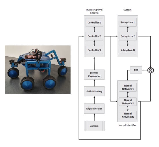
An Autonomous Path Controller in a System on Chip for Shrimp Robot

by
Sergio Barrios-dV
,
Michel Lopez-Franco
,
Jorge D. Rios
,
Nancy Arana-Daniel
,
Carlos Lopez-Franco
and
Alma Y. Alanis
*,†
Computer Sciences Department, University of Guadalajara, Blvd. Marcelino Garcia Barragan 1421, Guadalajara 44430, Mexico
*
Author to whom correspondence should be addressed.
These authors contributed equally to this work.
Electronics 2020, 9(3), 441; https://doi.org/10.3390/electronics9030441
Submission received: 23 January 2020 / Revised: 24 February 2020 / Accepted: 27 February 2020 / Published: 5 March 2020
(This article belongs to the Special Issue New Applications and Architectures Based on FPGA/SoC)

Abstract

:
This paper presents a path planning and trajectory tracking system for a BlueBotics Shrimp III®, which is an articulate mobile robot for rough terrain navigation. The system includes a decentralized neural inverse optimal controller, an inverse kinematic model, and a path-planning algorithm. The motor control is obtained based on a discrete-time recurrent high order neural network trained with an extended Kalman filter, and an inverse optimal controller designed without solving the Hamilton Jacobi Bellman equation. To operate the whole system in a real-time application, a Xilinx Zynq® System on Chip (SoC) is used. This implementation allows for a good performance and fast calculations in real-time, in a way that the robot can explore and navigate autonomously in unstructured environments. Therefore, this paper presents the design and implementation of a real-time system for robot navigation that integrates, in a Xilinx Zynq® System on Chip, algorithms of neural control, image processing, path planning, and inverse kinematics and trajectory tracking.

Graphical Abstract

1. Introduction

Currently, System on Chip (SoC) is an active research area due to its flexibility for real-time implementations in a wide area of applications, increasing the processing capability on hardware as well as the speed of processing information in real-time [1,2]. Furthermore, its applications range from image and video processing, which typically are time-consuming applications [1], as well as parametric identification and artificial intelligence implementations [2,3,4], energy systems applications [3,5], automatic control [2,4,5], among others. All of the above examples are real-time implementations that can be possible due to the great processing capability of SoC.
On the other hand, an autonomous path planning and following system are presented for a BlueBotics Shrimp III® (BlueBotics Shrimp III is a registered trademark of BlueBotics SA) (Figure 1). This robot is known for having terrain adaptability, thanks to its passive mechanical configuration, which gives it climbing abilities. These capabilities make it ideal for navigating in environments inaccessible or difficult for humans, useful for applications such as space exploration, rescue in catastrophe scenarios, firefighting, and remote inspection.
For this kind of application, it is useful to have a robot that has the ability to explore autonomously. For this purpose, this work presents a decentralized system that allows the robot to plan a route that avoids moving directly towards obstacles. Combined with its passive climbing ability, the shrimp robot will be capable of continuously exploring without human intervention.
One of the most critical issues in the design and development of an autonomous mobile robot is to provide it with the ability to plan and follow a path within its environment. However, this environment may be rough or non-structured. Robots need algorithms for data processing, recognition, interpreting, and decision making in order to navigate in an environment autonomously. Recently, machine learning has been applied to help mobile robots to improve these capabilities. Specifically, neural networks have proven to be very useful in these applications due to their capability to generalize learned behaviors to new circumstances. The interest in neural networks comes from the desire to understand and replicate basic human brain functions. Neural networks deal with cognitive tasks such as learning, adaptation, and optimization. They improve the adaptation capabilities related to variations in the environment where information is inaccurate, uncertain, or incomplete [6]. In the considered scenario, neural network capabilities are taken advantage of in two stages of the proposed autonomous robot system: to interpret visual information and to maintain the stability of an inverse optimal controller.
The full system scheme is presented in Figure 2. First, the environment is sensed by taking a photograph of the terrain; then, the image is interpreted as a map of obstacles using one of two methods: a Canny edge detector or a convolutional neural network. A path is planned using the obtained map [7]; then, an inverse kinematic model of the shrimp robot is used to transform the motion plan of the robot to the references of each motor, as in [8]. These references are followed by each motor using an inverse optimal controller, like the ones presented in [9,10]. Each plant is modeled using a neural identifier consisting of a recurrent high order neural network (RHONN) trained with an extended Kalman filter (EKF). A similar approach can be seen in [11,12,13,14]. All the above-mentioned works have presented results of simulation stage, or at most, they have achieved to execute parts of the navigation system (some algorithms, such as path planners, controllers, or image processing methods) on personal computers, and they send the outputs of the computer-executed-algorithms to the robot via Wi-Fi communication, which makes these systems highly susceptible to delays and most of the time impossible to be executed in real-time on robot platforms. Therefore, to the best of our knowledge, our proposal is the first fully autonomous navigation system that integrates algorithms of vision-based control, neural classification, path planning, neural identification, and inverse optimal control for the BlueBotics Shrimp III® robot platform. In addition, new kinematic modeling of the BlueBotics Shrimp III® robot is developed in this work to include the dynamics of each motor.
This work is organized as follows. First, the inverse optimal controller used in each motor is defined in Section 2. The kinematic model developed to describe the contribution of each motor to the velocity of the robot is detailed in Section 3. And the neural identifier used to model the system is described in Section 4. Section 5 describes the algorithm used to plan the path to be followed by the robot. In Section 6, implemented hardware is described. Section 7 shows real-time results of the proposed methodologies in two different unstructured environments. The conclusions about the work are discussed in Section 8.

2. Inverse Optimal Controller

Consider the following discrete time nonlinear system [15]:
x k + 1 = f x k + g x k u k , x 0 = x ( 0 )
where x k R n is the state of the system in time k Z + 0 = { 0 , 1 , 2 , } , u k R m is the input, f : R n R n and g : R n R n are smooth nonlinear functions. Assume that at x = 0 the system is in equilibrium, f ( 0 ) = 0 and g x k 0 x k 0 .
For such system, we need to determine a control law [16] u k = u ¯ x k , which minimizes the following cost function:
J x k = n = k l x n + u n K u n
where J : R n R + is a measure of performance; l : R n R + is a positive semi-definite weight function of state vector x k , and K : R is a symmetric positive definite weighting matrix of the control effort required. Elements of K can be constant or functions of state variables.
Equation (2) can be rewritten as:
J x k = l x k + u k R u k + n = k + 1 l x n + u n R u n
Therefore:
J x k = l x k + u k R u k + J x k + 1
when J x k is minimal, which is denoted as J x k , it is called optimal value function [17]. And complying with boundary condition J 0 = 0 , it can be used as a Lyapunov function: J x k V x k .
The optimization problem can be solved using Bellman’s principle of optimality. For optimization problems with infinite horizon, the optimal value function V x k is time invariable and complies with Bellman’s discrete-time equation [18].
V x k = min u k l x k + u k K u k + V x k + 1
The optimal control law u k is obtained by calculating the gradient regarding u k :
0 = 2 K u k + V x k + 1 u k = 2 K u k + g x k V x k + 1 x k + 1
Considering boundary condition V ( 0 ) = J ( 0 ) = 0 , the optimal control law is the following:
u k = 1 2 K 1 g T χ k V x k + 1 x k + 1
u k is used to emphasize that the control law u k is optimal.
By substituting the optimal control law in Bellman’s discrete time Equation (5), the discrete time Hamilton–Jacobi–Bellman (HJB) equation is obtained [19]:
0 = l x k + V x k + 1 V x k + 1 4 V x k + 1 x k + 1 g x k R 1 g T x k V x k + 1 x k + 1
Solving this equation of partial derivatives for V x k is not simple. This is one of the major disadvantages of applying discrete-time optimal control to nonlinear systems. To solve this problem control with inverse optimal control, a control-Lyapunov function is used to build an optimal control law directly, avoiding the need to solve the HJB equation [20,21].
The control law in Equation (7) is inverse optimal if it has global exponential stability in equilibrium point x k = 0 for System (1) and it minimizes the cost function defined as Equation (2) for which l x k : = V ¯ with:
V ¯ : = V x k + 1 V x k + u k K u k 0
Therefore, when l x k : = V ¯ , V ( x k ) is a solution for the HJB Equation (8). Inverse optimal control is based in knowing V ( x k ) , a control-Lyapunov function that guarantees that the control law is inverse optimal if matrix O is chosen appropriately:
V x k = 1 2 x k O x k , O = O > 0
Substituting the proposed V ( x k ) on the control law in Equation (7), the following is obtained:
u k = 1 2 K + 1 2 g x k O g x k 1 g x k O f x k
Note that matrices O and K are symmetric and positive so they have an inverse. The following theorem establishes a sufficient condition to choose a matrix O appropriately. Considering System (1), if a matrix O = O > 0 that complies with the following inequality:
V f x k 1 4 O 1 x k K + O 2 x k 1 O 1 x k ζ Q x k 2
where:
V f x k = V f x k V x k
V f x k = 1 2 f x k O f x k
O 1 x k = g x k O f x k
O 2 x k = 1 2 g x k O g x k
ζ Q is positive. Equilibrium point x k = 0 of System (1) is globally exponentially stabilized by the control law in Equation (11). Additionally, this control law is inverse optimal since it minimizes cost function in Equation (2) with l x k = V ¯ .
To model our nonlinear plant to be controlled, we used a neural identifier, as described in Section 4.

3. Shrimp’s Kinematic Model

The shrimp robot has two steered wheels, front and back, and four fixed wheels, two on the right side and two on the left. It has eight degrees of freedom (Figure 3), the velocity of each motor ( V F , V B , V R 1 , V R 2 , V L 1 , V L 2 ) and the angles of the steered wheels ( θ F , θ B ).
Considering the radius of each wheel as r, and the distance between the right wheels and left wheels defined by d. The relationship between linear speed (v) and angular speed ( ω ) of each wheel can be given as:
v = ω r
The summation of contributions of the linear speeds of each motor is used to calculate the linear velocity of the robot V s h r i m p = V F + V B + V R 1 + V R 2 + V L 1 + V L 2 . The frontal and back motor should have the same speed V F B = V F = V B , as well as both right motors V r = V R 1 = V R 2 and both left motors V L = V L 1 = V L 2 . The steering angle of the back motor should be the opposite of the front motor, θ = θ F = θ B . So, the linear velocity of the robot is defined as:
V s h r i m p = 2 V F B + 2 V R + 2 V L
Assuming that the robot moves forward [22], consider the contribution of right and left wheel angular speeds to the linear speed at the center of the robot. When a wheel on the right rotates and the left one on the same axis is at rest, there is no contribution of the left wheel to the speed of the robot, since the center is halfway between both wheels, the contribution of the right wheel is given by V R = r 2 ω r and similarly for the left wheels V L = r 2 ω l . The contribution to the robots velocity from the front and back wheels will be V F B = r 2 ω F B . Substituting in Equation (18), the robots linear velocity is determined by V s h r i m p = 2 r 2 R ω F B + 2 r 2 ω r + 2 r 2 ω l :
V s h r i m p = R ( ω F B + ω r + ω l )
To determine the angular speed of the robot, the contribution of each wheel is considered, when a right wheel is rotating forward, the robot turns in the counterclockwise direction, the angular speed can be computed because the robot is instantaneously moving the arc of a circle of radius d, where d is the distance between the right and left wheels ω 1 = R d ω r and when the left wheel is rotating forward then ω 2 = R d ω l . Given that L 2 is the distance between front and back motors, then ω 3 = R L 2 ω f b and ω 4 = R L 2 ω f b . The angular speed of the robot is:
ω s h r i m p = r L 1 ω r + r L 1 ω l + 2 r L 2 ω f b
Given the following:
x ˙ = V s h r i m p cos ( θ )
y ˙ = V s h r i m p sin ( θ )
θ ˙ = ω s h r i m p
Substituting the value of V s h r i m p and ω s h r i m p and utilizing matrix form:
x ˙ y ˙ ϕ ˙ = r cos ( θ ) r cos ( θ ) r cos ( θ ) r sin ( θ ) r sin ( θ ) r sin ( θ ) 2 r d 2 r d 1 r d 1 w f b w r w l
Using the pseudo-inverse of this matrix, the necessary reference signals for the motors from the desired velocity of the robot can be obtained. In Section 5, the methods used to determine the path the robot will take is described.

4. Neural Identifier

RHONNs have a dynamic behavior and high order interactions, which gave them great approximation properties, superior convergence capacity, better storage capacity, and larger fault tolerance than first-order networks [6,20,23]. Moreover, discrete-time and continuous-time recurrent high order neural networks have the same characteristics [20]. Neural networks have been widely used in control systems, mainly to deal with non-modeled dynamics in the available model of the system [24]. The way to use neural networks for control lies in two approaches: direct and indirect control. In the first one, the neural network is the controller for the system under study, and in the second approach, the neural network provides a dynamic model for the system to be controlled. Then, based on such neural model, a controller is designed using any desired control technique [24]. In this paper, the second approach is used, using a RHONN to design an identifier for discrete-time unknown nonlinear systems; this identifier provides a dynamic model that is then used to design an inverse optimal controller in order that the shrimp robot can follow the desired path in real-time.
Consider that System (1) has a perturbation:
x k + 1 = f x k + g x k u k + Γ k
where Γ k R n is an unknown bounded perturbation, which represents errors in modeling, uncertainties in parameters, and non-modeled dynamics. We assume that f ( 0 ) = 0 and that the rank of g x k is m for all x k 0 . To identify System (25), we consider the following discrete RHONN model [20]:
x ^ i , k + 1 = w i , k z i x ^ k + w i ψ i x ^ k , u k
where i = 1 , , n , x ^ k is the state of neuron i; w i , k is a weight vector adapted in line; w i is a fixed weight vector used to ensure controllability of the neural model; ψ i denotes a function of x ^ k or u ^ k that corresponds to the structure of Plant (25) or to the external input of the network, respectively. And u k = u 1 , k , u 2 , k , , u m , k is an input vector to the neural model; m is the number of external inputs; z i is a vector of dimension L p , and it is defined as:
z i x k = z i 1 z i 2 z i L p = j I 1 ξ i j d i j , 1 j I 2 ξ i j d i j , 2 j I L p ξ i j d i j , L p
where d j i , k is a positive integer; L p is the number of high order connections; and I 1 , I 2 , , I L p is a collection of non orderly subsets of { 1 , 2 , , n } , where n is the dimension of the state space. ξ i is a vector defined as:
ξ i = ξ i 1 ξ i n = S x 1 S x n
where the hyperbolic tangent function is chosen as S and ζ is a real variable:
S ( ζ ) = e ζ e ζ e ζ + e ζ = tan h ( ζ )
It is assumed that a RHONN models System (25) exists based on [23]; therefore, the plant model is redefined as:
x k + 1 = W k z x k + W ψ x k , u k + ϵ k
where the following are unknown optimal weighting matrices:
W k = w 1 , k , w 2 , k , , w n , k
W = w 1 , w 2 , , w n
And the modeled error is the following:
ϵ k = f x k + g x k u k + Γ k W k z x k W ψ x k , u k
The term ϵ k can be made arbitrarily small and by selecting appropriately the number of high order connections L p [25]. Weighting matrices w i , k will be approximated with adapted weighting vectors in line w i , k .
For the training of neural networks, using an extended Kalman filter algorithm, the state variables to be estimated are the weights of the neural network. In this case, the error between the outputs of the neural network and the output of the plant can be considered white noise. A Kalman filter estimates the state of a linear system perturbed by white noise in its state and its output [26]. Since the mapping of the neural network is nonlinear, an extended Kalman filter is used instead of [27].
The objective of the training is to find optimal values of weights, which minimize errors in prediction. The algorithm for EKF is the following:
K k = P k H k R k + H k P k H k 1
w k + 1 = w k + η K k y k y ^ k
P k + 1 = P k K k H k P k + Q k
where P R R L × L is the covariance matrix associated to the prediction error; w R L is the weight vector, L is the total number of weights, y R n is the measured output, y ^ R n is the output of the network, η is a design parameter; K R L × n is the Kalman matrix of gains; Q R L × L is the matrix of covariance associated with noise in the state, R R n × n in the covariance matrix associated with the noise in the measurements; H R L × n is a matrix for which every input H i j is a derivative of each output of the neural network with respect to each weight, as defined in the following equation:
H i j ( k ) = y ^ i ( k ) w j ( k ) w ^ i ( k + 1 ) = w i ( k )
where:
i = 1 , , n
j = 1 , , L
Usually, P, Q, and R are initialized with diagonal matrices with inputs P 0 , Q 0 , and R 0 [28]. With each motor being modeled and controlled, the contribution of each one to the movement of the robot has to be determined. For this purpose, a kinematic model, as described in Section 3, is used.

5. Path Planning

In order to plan a path for the robot, a camera senses the surroundings by capturing an 800 by 600 pixels image. Based on that image, a map of the surroundings of the robot is obtained. Then, the map is used to determine the possible route to arrive at a goal point. To process the image, two methods are implemented. The first uses traditional edge detector algorithms to identify possible obstacles or patches of rough terrain. The second method utilizes machine learning techniques to classify segments of the image into possible paths or obstacles.
In the first method, possible obstacles or rough terrain are detected by looking for the edges using a Canny edge detector, which has been widely adopted due to its reliable performance in noisy environments [29]. The Canny detector is known as the optimal detector; it has a low error rate, and it minimizes the distance between detected edge pixels and real edge pixels [30].
For this detector, noise is filtered with a Gaussian filter. Then, the intensity gradient of the image is found. Hysteresis is used to suppress pixels not considered to be part of the edges; two thresholds are used. If a pixel gradient is higher than the upper threshold, it is accepted as an edge. If it is under the lower threshold, then it is not an edge. Pixels in the middle are accepted if it is next to an edge pixel. The resulting matrix is resized to 80 by 60. Edges are considered obstacles.
In the second method, the image is split into 80 by 60 squares; each is classified as either obstacle or possible path using a convolutional neural network (CNN), the classifier was implemented using Google opensource library TensorFlow [31]. A sequential model is used with three convolutional blocks, a fully connected layer, and an output layer with a sigmoidal activation function. The output is the probability that the segment of the image contains an obstacle; every square with a higher than average probability is considered an obstacle on the map. The latter is filtered to reduce the noise of false positives.
Before it can be used on the robot, a model has to be trained on a database. This database is augmented by flipping, rotating, and scaling each picture. And more importantly, each picture is used with different levels of light by normalizing its intensity around ten different ranges. This step is essential since it makes the model robust to differences in illumination. The model is trained over the entire database of 1700 images over 50 times; this gives us an accuracy of 89 percent.
Using a neural network is more robust and resistant to differences in illumination compared to using an edge detector. However, even with the model being trained previously on a PC, it takes considerably more computing time when implemented on an embedded platform.
Regardless of which method is used, the resulting map is run through a grid-based shortest path planning algorithm [32]. The system uses Dijkstra’s algorithm, where each square of the grid is a node [33]; it has been selected due to the fact that it can guarantee an optimal plan even when the distance to the target is not known. The algorithm starts from an initial node that is assigned a distance of zero, and the rest are assigned an infinite distance. The distance between the current nodes and its neighbors is established, and if it is shorter than the currently saved distance, then it is replaced. When all neighbors of a current node have been visited, then its distance is considered final. Then you move to the next non-visited node with the lowest distance. This variant of the algorithm ends when a target node is reached [34].
The path planning and control system, described above, have been implemented on the Shrimp robot using the hardware described in the following section.

6. Hardware Implementation

The final design consists of the mechanics and power electronics of the BlueBotics Shrimp III® autonomous robot, a PYNQ-Z1 board with a Xilinx Zynq® (Xilinx Zynq is a registered trademark of Xilinx, Inc.) Z7020 System-on-Chip for control and path tracking, and an STMicroelectronics NUCLEO-F746ZG board with an STM32F746ZG Micro-Controller Unit (MCU) for communication. The electric diagram is presented in Figure 4.

6.1. BlueBotics Shrimp III

The Shrimp III® was designed by BlueBotics as a research platform for rough terrain with applications on space exploration, rescue work on catastrophic scenarios, assistance in firefighting, and remote inspection.
BlueBotics Shrimp III® has a completely passive climbing structure that allows it to move through rough terrain and to climb small obstacles, while the control unit simply instructs it to move forward. It consists of two wheels on the right side, two on the left side, a steered wheel for the front, and a steered wheel in the back. The steering has a range of 180 degrees. The robot is manipulated with commands through rs232 communication.

6.2. Xilinx PYNQ-Z1

The PYNQ-Z1 board is used as the main control unit. Zynq® Z7020 SoC includes a Dual-core ARM Cortex-A9 Micro-Procesor HardCore, as well as programmable logic cells capable of functioning as several Microblaze SoftCores for extra general-purpose processing or as application-specific hardware. The hardcore is capable of running a small version of Linux and a python interpreter. Python® (“Python” is a registered trademark of the PSF) allows for quick development and deployment of a control system while computing-intensive tasks, it can be resolved in application-specific accelerators implemented on programmable logic to achieve processing times adequate for a real-time application.

6.3. STMicroelectronics NUCLEO-F746ZG

The Nucleo F746ZG board is used for communication. It is an ARM® 32-bit Cortex®-M7 CPU running at 216 MHz, its high speed allows for a low latency data transfer between this board and the Zynq® board used as the main processing unit. The latter lacks the universal asynchronous receiver-transmitter (UART) necessary to communicate directly with the shrimp robot. Although the SoC is capable of synthesizing such transmitter, at the moment, such implementation has a fixed baud rate of 9600 bits per second, which is not compatible with the shrimp robot. Instead, the Nucleo F746ZG board is connected through MAX232 drivers with the robot at 56,200 bits per second. The received data is passed to the Zynq® board using parallel General Purpose Input/Output (GPIO). An 8-bit output bus is used as well as a request output flag and an acknowledge input. A similar interface is used in the opposite direction as a means of passing shrimp’s responses.

7. Results

In this section, experimental results for the integration of vision-based control, path planning, neural identification, and inverse optimal controller all integrated and working together in an unstructured environment, have been included in order to show the effectiveness of the proposed methodology. In addition, a comparative analysis of the proposed methodology implemented in SoC and the same methodology implemented in a personal computer (PC) has been included, considering advantages and disadvantages of both kinds of implementations.

7.1. Experimental Results

The system was tested in different unstructured environments. The first one can be seen in Figure 5, which contains rough terrain to be dodged.
As mentioned earlier, this photograph can be processed in two different ways. When using the edge detector, the image presented in Figure 6 is obtained. Once processed by the path planning algorithm, the path in Figure 7 is obtained. Similarly, Figure 8 shows the map and planned path using CNN. Expected planned paths with both methods on the original photograph are shown in Figure 9 and Figure 10, respectively.
Another example is presented in Figure 11, where the path forward is through a ramp. The result of the edge detector, in this case, is shown in Figure 12. The calculated path using the Canny edge detector is shown as a red line in Figure 13, and the one calculated with a CNN in Figure 14 also as a red line. Both can be seen overlaid on the original photographs on Figure 15 and Figure 16, respectively.
Once the path has been planned, the required speed of each motor to follow the path is calculated and used as the reference signal for the motors control using the inverse optimal control methodology described above. Figure 17 shows the results of each controller using for the route on Experiment 1 for frontal, left, right, and back motors, respectively. Results for the second case can be seen in Figure 18 for frontal, left, right, and back motors, respectively. It is important to note that applied voltages remain bounded and depends on the difficulty defined by the path planning route, in Experiment 2, applied voltages are bigger than the applied voltage for Experiment 1, this is due to the slope of the rough terrain and the kind of path defined by the proposed algorithm.
It is important to remark that the main goal of this paper lies on the integration of vision-based control, path planning, neural identification, and inverse optimal controller all integrated and working together using a Xilinx Zynq® System on Chip. In the literature, the latest algorithms can be found working alone mainly in software. Our main contribution is on the integration of a whole full autonomous system in a shrimp robot for 3D autonomous navigation in difficult, unstructured environments, and in this way, the literature does not report similar works that can be compared with our proposed scheme. In addition, hardware limitations do not allow us to implement more complex algorithms for each stage.

7.2. Comparative Analysis

It is well known that a SoC is an integrated circuit with all components of a PC, and its use has advantages and disadvantages. The main advantage is autonomy, as it allows to integrate in a mobile system all the processing power that it is required to achieve its target, improving its processing time, avoiding delays and other communication problems, due to the fact that the processor is mounted directly in the system, in this case, in the mobile robot platform, allowing it to navigate autonomously on unstructured environments. However, the limited processing capabilities and limited available memory that can be used for the desired application can be considered as a disadvantage.
In order to include a comparative analysis of the obtained performance in SoC with respect to a PC, the same experiments have been implemented in both kinds of platforms, with two different algorithms for path planning A* and Dijkstra with the results presented in Table 1 and Table 2 for Experiments 1 and 2, respectively. As is expected, the PC has a better processing performance compared with respect to the SoC proposed methodology. However, for real-time autonomous navigation on unstructured environments, SoC is a better option.
Results presented in Figure 5, Figure 6, Figure 7, Figure 8, Figure 9, Figure 10, Figure 11, Figure 12, Figure 13, Figure 14, Figure 15, Figure 16, Figure 17 and Figure 18 have been obtained with Dijkstra’s algorithm and does not need to know the destination node a priory, which facilitates real-time navigation in unstructured environments and is one of the main goals of this work, meaning it was our best option for the proposed implementation.
The required time to compute the route varies depending on the input taken by the camera, as well as other processes running on the operating system of the Xilinx Zynq® SoC. In the case of Experiment 1, when using an edge detector, it takes 68.34 s before the motion can start with 59.83 s spent in Dijkstra’s algorithm and 7.25 s on the Canny edge detector. Actual movement through the route takes 123.54 s.
On Experiment 2, processing takes 84.27 s, and route calculation accounts for most of the difference taking 76.01 s, while edge detection only takes 6.87 s. Movement through the route takes 113.36 s. In general, the system takes approximately a third of its time processing and the rest in motion.
It is important to note that both implementations have been developed using Python®. For PC implementation a PC with a processor Intel® (Intel is a trademark of Intel Corporation or its subsidiaries) i5-8250U CPU @ 1.6 GHz and 16.0 GB of RAM was selected. In addition, a latency analysis with the following ping statistical information has been done. Packages: sent = 100, received = 98, lost = 2. Approximate round trip times in milliseconds: Minimum = 1 ms, Maximum = 799 ms, Average = 15 ms.
It is important to note that even when a PC has more resources to process than a SoC, both of them present advantages and disadvantages. For example, the use of a PC allows to perform faster information processing; however, it needs the use of a Wi-Fi connection, which it is not always possible to have in unstructured environments. Furthermore, this kind of connection is typically affected by problems like delays, pocket lost, and interference, among others, restricting robot autonomy for navigation. Due to the limited payload of this kind of robot, it is not possible to install a PC above of the shrimp robot, and as a result, this situation cannot be considered in order to avoid the use of Wi-Fi.
As explained above, a work that integrates all the elements considered in this paper is not reported in the literature; therefore, we only can compare each one of the proposed elements with respect to similar approaches implemented in the same robot in an independent way. In [35], a similar controller in an Altera Cyclone® (“Altera and Cyclone” are registered trademarks of Altera Co.) IV EP4CE115F29C7 FPGA is implemented; however, such FPGA only supports controller processing without image processing, path planning, nor visual-based control. In [36], a path planning based on a long short-term memory (LSTM) neural network is proposed, which can give better performance; however, it is computationally expensive and, therefore, it cannot be applied on-line, as is the path planning proposed in this paper. Finally, for image processing, in Section 5, a Canny detector against a CNN obstacle classifier is compared, the last of them showing better performance; however, again, it is computationally expensive, and it cannot be applied on-line. For all the above comparisons, in order to have a system that can explore autonomously in unstructured environments based on a shrimp robot, the better solution, considering performance, economy, flexibility and processing capability, is the implementation of the vision-based control, path planning, neural identification, and inverse optimal controller all integrated and working together using a Xilinx Zynq® System on Chip.

8. Conclusions

The vision-based path planning and trajectory tracking neural controller implemented in this paper is an adequate solution to grant a shrimp robot the capability to explore difficult environments autonomously.
The system on chip implementation allows for excellent performance and fast calculations. Using the CNN classifier to determine obstacles is an excellent way to better handle differences in illumination but is computationally intensive compared with using the Canny edge detector. The former is particularly useful when there is a PC on the loop to co-process the classification or if it is not a problem for the robot to remain idle while processing. The Dijkstra algorithm is also a computationally intensive step; in Section 7.2, a comparison with A* has been included, with a better processing time than the Dijkstra algorithm; however, the last one presents a better performance in the experimental results considered in Section 7.1.
From the presented results in Section 7.1, the systems plan a path avoiding more difficult terrain, preventing the shrimp from running into obstacles than can not be overcome by its passive climbing mechanism. The path is then followed by having each motor follow its necessary contribution to the movement of the robot as determined by the developed kinematic model. Each motor follows its reference closely with the implemented inverse optimal controller in which the plant is modeled with an RHONN trained with EKF.

Author Contributions

Conceptualization, S.B.-d. and M.L.-F.; formal analysis, J.D.R. and A.Y.A.; funding acquisition, A.Y.A. and N.A.-D.; investigation, C.L.-F. and N.A.-D.; methodology, S.B.-d.; project administration, A.Y.A.; software, S.B.-d. and M.L.-F.; supervision, A.Y.A. and J.D.R.; validation, C.L.-F.; writing—original draft, S.B.-d. and A.Y.A.; writing—review and editing, J.D.R. and A.Y.A. All authors have read and agree to the published version of the manuscript.

Funding

The authors thank the support of CONACYT México, through Projects CB-2015-256769, CB-2015-258068, and PN-2016-4107. (“Project supported by Fondo Sectorial de Investigación para la Educación ).

Acknowledgments

The authors thank the support of CUCEI, University of Guadalajara.

Conflicts of Interest

The authors declare that there is no conflict of interest regarding the publication of this paper.

Abbreviations

The following abbreviations are used in this manuscript:
RHONNRecurrent High Order Neural Network
EKFExtended Kalman Filter
HJBHamilton–Jacobi–Bellman
CNNConvolutional Neural Network
CEDCanny Edge Detector

References

  1. Bravo-Muñoz, I.; Lázaro-Galilea, J.L.; Gardel-Vicente, A. FPGA and SoC Devices Applied to New Trends in Image/Video and Signal Processing Fields. Electronics 2017, 6, 25. [Google Scholar] [CrossRef] [Green Version]
  2. Ge, F.; Wu, N.; Xiao, H.; Zhang, Y.; Zhou, F. Compact Convolutional Neural Network Accelerator for IoT Endpoint SoC. Electronics 2019, 8, 497. [Google Scholar] [CrossRef] [Green Version]
  3. Lai, X.; Yi, W.; Zheng, Y.; Zhou, L. An All-Region State-of-Charge Estimator Based on Global Particle Swarm Optimization and Improved Extended Kalman Filter for Lithium-Ion Batteries. Electronics 2018, 6, 321. [Google Scholar] [CrossRef] [Green Version]
  4. Renteria-Cedano, J.; Rivera, J.; Sandoval-Ibarra, F.; Ortega-Cisneros, S.; Loo-Yau, R. SoC Design Based on a FPGA for a Configurable Neural Network Trained by Means of an EKF. Electronics 2019, 8, 761. [Google Scholar] [CrossRef] [Green Version]
  5. Ricco, M.; Mathe, L.; Hammami, M.; Franco, F.L.; Rossi, C.; Teodorescu, R. AA Capacitor Voltage Balancing Approach Based on Mapping Strategy for MMC Applications. Electronics 2019, 8, 449. [Google Scholar] [CrossRef] [Green Version]
  6. Sanchez, E.N.; Alanis, A.Y.; Loukianov, A.G. Discrete Time High Order Neural Control; Springer: Berlin, Germany, 2008. [Google Scholar]
  7. Roka, R. Advanced Path Planning for Mobile Entities, 1st ed.; IntechOpen: London, UK, 2018. [Google Scholar]
  8. Lopez-Franco, C.; Hernandez-Barragan, J.; Alanis, A.Y.; Arana-Daniel, N. A soft computing approach for inverse kinematics of robot manipulators. Eng. Appl. Artif. Intell. 2018, 74, 104–120. [Google Scholar] [CrossRef]
  9. Lastire, E.A.; Sanchez, E.N.; Alanis, A.Y.; Ornelas-Tellez, F. Passivity analysis of discrete-time inverse optimal control for trajectory tracking. J. Frankl. Inst. 2016, 353, 3192–3206. [Google Scholar] [CrossRef]
  10. Rios, J.D.; Alanis, A.Y.; Lopez-Franco, M.; Lopez-Franco, C.; Arana-Daniel, N. Real-time neural identification and inverse optimal control for a tracked robot. Adv. Mech. Eng. 2017, 9. [Google Scholar] [CrossRef] [Green Version]
  11. Rios, J.D.; Alanis, A.Y.; Arana-Daniel, N.; Lopez-Franco, C. Neural Identifier-Control Scheme for Nonlinear Discrete Systems with Input Delay. In Fuzzy Logic in Intelligent System Design; Melin, P., Castillo, O., Kacprzyk, J., Reformat, M., Melek, W., Eds.; Springer International Publishing: Berlin, Germany, 2018; pp. 242–247. [Google Scholar]
  12. Vazquez, L.A.; Jurado, F.; Castañeda, C.E.; Alanis, A.Y. Real-Time Implementation of a Neural Integrator Backstepping Control via Recurrent Wavelet First Order Neural Network. Neural Process. Lett. 2018. [Google Scholar] [CrossRef]
  13. Alanis, A.Y.; Sanchez, E.N. Discrete-Time Neural Observers: Analysis and Applications, 1st ed.; Academic Press: London, UK, 2017. [Google Scholar]
  14. Rios, J.D.; Alanis, A.Y.; Lopez-Franco, C.; Arana-Daniel, N. RHONN identifier-control scheme for nonlinear discrete-time systems with unknown time-delays. J. Frankl. Inst. 2017, 355, 218–249. [Google Scholar] [CrossRef]
  15. Sanchez, E.N.; Ornelas-Tellez, F. Discrete-Time Inverse Optimal Control for Nonlinear Systems; CRC Press: New York, NY, USA, 2013. [Google Scholar]
  16. Kirk, D.E. Optimal Control Theory. An Introduction; Dover Publications, Inc.: New York, NY, USA, 2014. [Google Scholar]
  17. Al-Tamimi, A.; Lewis, F.L.; Abu-Khalaf, M. Discrete-time nonlinear HJB solution using approximate dynamic programming: Convergence proof. IEEE Trans. Syst. Man Cybern. 2008, 38, 943–949. [Google Scholar] [CrossRef] [PubMed]
  18. Sun, J.; Krstic, M.; Bekiaris-Liberis, N. Robust adaptive control: Legacies and horizons. Int. J. Adapt. Control Signal Process. 2012, 27. [Google Scholar] [CrossRef] [Green Version]
  19. Camacho, O.; Fridman, L.; Chairez, I. Discrete time super-twisting observer for 2n dimensional systems. In Proceedings of the 8th International Conference on Electrical Engineering Computing Science and Automatic Control 2011 (CCE), Merida City, Mexico, 26–28 October 2011; pp. 1–6. [Google Scholar]
  20. Sanchez, E.N.; Ornelas-Tellez, F.; Loukianov, A.G. Discrete-time neural inverse optimal control for nonlinear systems via passivation. IEEE Trans. Neural Netw. Learn. Syst. 2012, 23, 1327–1339. [Google Scholar]
  21. Lopez-Franco, M.; Sanchez, E.N.; Alanis, A.Y.; Arana-Daniel, N. Real-time decentralized inverse optimal neural control for a Shrimp robot. In Proceedings of the 2013 International Joint Conference on Neural Networks (IJCNN), Dallas, TX, USA, 4–9 August 2013; pp. 1–7. [Google Scholar] [CrossRef]
  22. Diriba, B.; Zhongmin, W. Design and Control for Differential Drive Mobile Robot. Int. J. Eng. Res. Technol. (IJERT) 2017, 6, 327–334. [Google Scholar]
  23. Kutz, M. Mechanical Engineers’ Handbook, Volume 2: Design, Instrumentation, and Controls; Wiley: Bethlehem, PA, USA, 2015. [Google Scholar]
  24. Norgaard, M. Neural Networks for Modelling and Control of Dynamic Systems: A Practitioner’s Handbook; Springer: Berlin, Germany, 2003. [Google Scholar]
  25. Lewis, F.L.; Vrabie, D.L.; Syrmos, V.L. Optimal Control; John Wiley and Sons: New York, NY, USA, 2012. [Google Scholar]
  26. Grover, R.; Hwang, P.Y.C. Introduction to Random Signals and Applied Kalman Filtering with Matlab Exercises; John Wiley and Sons: New York, NY, USA, 2012. [Google Scholar]
  27. Alanis, A.Y.; Sanchez, E.N.; Loukianov, A.G. Discrete-time adaptive backstepping nonlinear control via high-order nerual networks. IEEE Trans. Neural Netw. Learn. Syst. 2007, 18, 1185–1195. [Google Scholar] [CrossRef] [PubMed]
  28. Barrau, A.; Bonnabel, S. The Invariant Extended Kalman Filter as a Stable Observer. IEEE Trans. Autom. Control 2014, 62. [Google Scholar] [CrossRef] [Green Version]
  29. Lee, J.; Tang, H.; Park, J. Energy Efficient Canny Edge Detector for Advanced Mobile Vision Applications. IEEE Trans. Circuits Syst. Video Technol. 2018, 28, 1037–1046. [Google Scholar] [CrossRef]
  30. Kapur, S. Computer Vision with Python 3; Packt Publishing: Birmingham, UK, 2017. [Google Scholar]
  31. Ertam, F.; Aydın, G. Data classification with deep learning using Tensorflow. In Proceedings of the 2017 International Conference on Computer Science and Engineering (UBMK), Antalya, Turkey, 5–8 October 2017; pp. 755–758. [Google Scholar] [CrossRef]
  32. Sariff, N.; Buniyamin, N. An Overview of Autonomous Mobile Robot Path Planning Algorithms. In Proceedings of the 4th Student Conference on Research and Development (2006), Selangor, Malaysia, 27–28 June 2006; pp. 183–188. [Google Scholar]
  33. Cormen, T.H.; Leiserson, C.E.; Rivest, R.L.; Stein, C. Introduction to Algorithms; MIT Press: Cambridge, MA, USA, 2009; pp. 595–601. [Google Scholar]
  34. Sakai, A.; Ingram, D.; Dinius, J.; Chawla, K.; Raffin, A.; Paques, A. PythonRobotics: A Python Code Collection of Robotics Algorithms. 2018. Available online: http://xxx.lanl.gov/abs/1808.10703 (accessed on 15 January 2020).
  35. Quintal, G.; Sanchez, E.N.; Alanis, A.Y.; Arana-Daniel, N.G. Real-time FPGA Decentralized Inverse Optimal Neural Control for a Shrimp Robot. In Proceedings of the 2015 10th System of Systems Engineering Conference (SoSE), San Antonio, TX, USA, 17–20 May 2015. [Google Scholar]
  36. Arana-Daniel, N.; Alanis, A.Y.; Lopez-Franco, C. Artificial Neural Networks for Robotics an Engineering Perspective; CRC Press: Boca Raton, FL, USA, 2019. [Google Scholar]
Figure 1. BlueBotics Shrimp III®.
Electronics 09 00441 g001
Figure 2. Design of the path planning and following system.
Electronics 09 00441 g002
Figure 3. Degrees of freedom of the Shrimp robot. The velocity of front motor ( V F ), back motor ( V B ), two right motors ( V R 1 , V R 2 ), and two left motors ( V L 1 , V L 2 ), and the angles of the steered front and back wheels ( θ F , θ B ).
Electronics 09 00441 g003
Figure 4. Electric schematic.
Electronics 09 00441 g004
Figure 5. Experiment 1. Image captured with the camera.
Electronics 09 00441 g005
Figure 6. Experiment 1. Results of the Canny edge detector.
Electronics 09 00441 g006
Figure 7. Experiment 1. Map and path planned using a Canny edge detector.
Electronics 09 00441 g007
Figure 8. Experiment 1. Map and path planned using a convolutional neural network (CNN).
Electronics 09 00441 g008
Figure 9. Experiment 1. Map and path planned using Canny edge detector overlaid on the original photograph.
Electronics 09 00441 g009
Figure 10. Experiment 1. Map and path planned using CNN overlaid on the original photograph.
Electronics 09 00441 g010
Figure 11. Experiment 2. Image captured with the camera.
Electronics 09 00441 g011
Figure 12. Experiment 2. Results of the Canny edge detector.
Electronics 09 00441 g012
Figure 13. Experiment 2. Map and path planned using Canny edge detector.
Electronics 09 00441 g013
Figure 14. Experiment 2. Map and path planned using CNN.
Electronics 09 00441 g014
Figure 15. Experiment 2. Map and path planned using Canny edge detector overlaid on the original photograph.
Electronics 09 00441 g015
Figure 16. Experiment 2. Map and path planned using CNN overlaid on the original photograph.
Electronics 09 00441 g016
Figure 17. Applied input voltage for Experiment 1.
Electronics 09 00441 g017
Figure 18. Applied input voltage for Experiment 2.
Electronics 09 00441 g018
Table 1. Processing times for Experiment 1.
Process TimeDijkstra in PCA* in PCDijkstra in SoCA* in SoC
Total time51.5293 s39.0263 s192.3780 s161.4557 s
Edge detector time0.6654 s0.5661 s7.2546 s7.3049 s
Map time0.0846 s0.0859 s1.0832 s1.0992 s
Route time15.5700 s3.9897 s60.1439 s28.9141 s
Control time0.0430 s0.0152 s0.3516 s0.3335 s
Time to start motion16.3631 s4.6571 s68.8334 s37.6519 s
Movement in route35.1661 s34.3692 s123.5445 s123.8038 s
Table 2. Processing times for Experiment 2.
Process TimeDijkstra in PCA* in PCDijkstra in SoCA* in SoC
Total time53.9585 s37.6130 s197.6433 s150.2245 s
Edge detector time0.6343 s0.6338 s6.8708 s7.2072 s
Map time0.0922 s0.1002 s1.0592 s1.0576 s
Route time21.3259 s5.0940 s76.0095 s29.4022 s
Control time0.0178 s0.0134 s0.3348 s0.3397 s
Time to start motion22.0704 s5.8416 s84.2744 s38.0069 s
Movement in route31.8881 s31.7714 s113.3688 s112.2176 s

