Design of Novel Nested Arrays Based on the Concept of Sum-Difference Coarray

1. Introduction

Direction of arrival (DOA) estimation of multiple signals is a hot topic in the area of array signal processing since it can be widely used in radar, sonar, and remote diagnosis, etc. [1,2,3,4,5]. In the past few decades, many subspace-based methods, such as multiple signal classification (MUSIC) [6], estimation of signal parameters via rotational invariance technique (ESPRIT) [7], and their modifications, have been proposed to address the DOA estimation problem. However, to avoid spectrum aliasing, inter-element spacing of the received array such as traditional uniform linear array (ULA) is restricted to not more than half a wavelength of the signals. Consequently, the aforementioned methods used on such ULA with $N$ sensors can only resolve $N-1$ sources, i.e., the overdetermined DOA estimation [8].

However, more and more situations concerning underdetermined DOA estimation, where the number of incident signals exceeds that of physical sensors, have been encountered in practical applications such as 5G wireless communication [9]. Many sparse arrays, whose inter-element spacing can break the half-wavelength restriction, have been presented to handle this underdetermined DOA estimation problem. Relying on the difference coarray (DCA) concept [8,10], they can construct virtual arrays with increased degrees of freedom (DOFs). Furthermore, compared with traditional ULA with $N$ sensors, sparse arrays with the same number of sensors possess larger physical apertures due to the increase of inter-element spacing. Thus, the DOA estimation performance of these sparse arrays is significantly better than that of traditional ULA.

Minimum redundancy array (MRA) [11] and minimum hole array (MHA) [12] are two kinds of typical sparse arrays. While both of them can be used to identify more sources than sensors, they do not have the closed-form expressions for their geometries and virtual arrays. As a result, sensor positions of MRA and MHA for the given sensor number $N$ are obtained through the enumeration method. Recently, nested array (NA) [8] and coprime array (CPA) [13] are also proposed for underdetermined DOA estimation. Research results indicate that sensor positions of NA and CPA can be determined easily owing to the existence of closed-form expressions for their physical structures.

To improve the detection performance of CPA and NA, many modified versions of them are proposed as well. For example, generalized CPA [14] and CPA with multiperiod subarrays [15] are designed to fill in the holes of virtual arrays and thus increase the available continuous DOFs. By contrast, thinned CPA (TCPA) proposed in [16,17] removes the redundant physical sensors without reducing the DOFs of virtual array. In addition, lots of modified NAs have also been presented to increase the continuous DOFs. By redesigning the structures of subarrays in NA, some modifications, such as improved NA [18] and augmented NA [19], are developed, which own higher continuous DOFs than the prototype NA. Meanwhile, the generalized nested subarrays reported in [20,21] have advantages in increasing the DOFs and physical apertures, which can also be termed as robust NAs. Note that, the virtual arrays of CPA and its modifications are discontinuous, which indicates that they cannot be totally used for DOA estimation when the subspace-based methods are employed [10]. On the other hand, although the modified NAs mentioned above have continuous virtual arrays with increased DOFs, they still have some limitations since only DCAs are included in their virtual arrays.

In recent years, sum coarray (SCA) of sparse array has attracted much attention since it can improve the DOA estimation performance [22,23,24,25,26]. More specifically, to obtain the virtual array composed of sum-difference coarray (SDCA) in a passive DOA estimation system, researchers in [22] utilized the spatial and temporal information jointly to design a vectorized conjugate augmented MUSIC (VCAM) method. By using the elements of SCA to fill in the holes of DCA, the VCAM method can achieve the increase of continuous DOFs and thus improve the detection performance of CPA. Accordingly, an improved CPA based on the SDCA concept is presented in [26], which can reduce the mutual coupling effect and increase the physical aperture, but there are still holes existing in its virtual array. In [24], by jointly exploiting the DCA and SCA, the authors designed a diff-sum NA (DsNA), which can increase the continuous DOFs and physical aperture at the same time. Similarly, in our previous work, we have proposed two improved NAs with SDCAs (i.e., INAwSDCA-I and INAwSDCA-II) [25]. By translating the subarrays of $N$-sensor NA and then flipping part of sensors, both INAwSDCA-I and INAwSDCA-II can generate $\mathrm{O}\left(N^2+3N\right)$ continuous DOFs and their physical apertures can also be increased dramatically.

Unfortunately, from Reference [25], we find that there exist holes in the SDCA of INAwSDCA-I, which means it cannot be completely utilized for DOA estimation. Although INAwSDCA-II can generate a fully continuous SDCA, there still exists redundancy in its physical structure. Consequently, the structures of INAwSDCA-I and INAwSDCA-II are not the optimal and can be further improved. To remove the redundancy and obtain the fully continuous SDCA, we propose four novel nested arrays (NNAs) based on the SDCA concept. In comparison with other sparse arrays, the proposed structures possess larger physical apertures and can generate the same SDCA with significantly increased continuous DOFs. By introducing the translational NA [25] and modifying it, we first propose the modified translational NA (MTNA). The property of MTNA indicates that its SDCA possesses increased continuous DOFs, which can be used to improve the DOA estimation performance. Then, through the systematic analysis of MTNA and its SDCA, we find that two different parts in the subarrays of MTNA can be removed. Thus, there exist four different NNAs with the same virtual array and different physical apertures. To generate the desirable SDCA from the above NNAs, different index sets used to construct the time average vectors are designed. Meanwhile, the closed-form expressions of the proposed arrays and SDCA are derived as well, which can help to construct the satisfying structures of NNAs. Simulation results are provided to demonstrate the superiority of the proposed arrays.

To be more specific, the main contributions of this paper are summarized as follows:

• By jointly exploiting the spatial and temporal information of received data, SDCA of a physical array is constructed, which can contribute to the increase of continuous DOFs. Moreover, its generation process has been discussed detailedly in this paper. And, we have also given the definition of two index sets, whose role is to construct the desirable time average vector and the corresponding equivalent received array.
• Four NNAs are proposed in this paper to achieve the purpose of improving the underdetermined DOA estimation performance. Specifically, they possess different physical apertures, but can generate the same SDCA for DOA estimation.
• The closed-form expressions for the proposed NNAs and their SDCA are provided in this paper. Moreover, the specific expressions for the index sets corresponding to different NNAs are also presented. These expressions can make it easy for readers to design the NNAs they want to use.

The remainder of this paper is arranged as follows. Section 2 introduces the VCAM method and two useful definitions. Section 3 gives the MTNA structure first, then shows the results of redundancy analysis about MTNA, and finally introduces the proposed array configurations as well as their properties. Section 4 provides the simulation results and Section 5 concludes this paper.

2. System Model

Consider $K$ far-field narrowband signals from directions $\left\{{\theta }_1,{\theta }_2,\cdots ,{\theta }_K\right\}$ impinging on a $N$-sensor linear array, whose sensor positions can be denoted as:

$$\mathbb{L}=\mathbb{S}d=\left\{s_1,s_2,\cdots ,s_N\right\}d,$$

(1)

where $\mathbb{S}\subseteq \mathbb{Z}$, and $\mathbb{Z}$ is the integer set. Without loss of generality, the unit inter-element spacing $d$ is set to be half a wavelength of received signals. For convenience, $d$ is ignored in this paper.

Accordingly, we can express the received data of the $t$-th snapshot as:

$$\mathit{x}\left(t\right)=\mathit{A}\mathit{s}\left(t\right)+\mathit{n}\left(t\right),$$

(2)

where $\mathit{A}=\left[\mathit{a}\left({\theta }_1\right),\mathit{a}\left({\theta }_2\right),\cdots ,\mathit{a}\left({\theta }_K\right)\right]$, $\mathit{s}\left(t\right)$, and $\mathit{n}\left(t\right)$ respectively denote the array manifold matrix, signal vector, and noise vector. $\mathit{a}\left({\theta }_k\right)={\left[e^{j\pi s_1\sin \left({\theta }_k\right)},e^{j\pi s_2\sin \left({\theta }_k\right)},\cdots ,e^{j\pi s_N\sin \left({\theta }_k\right)}\right]}^{\mathrm{T}}$ is the steering vector associated with ${\theta }_k$ and the superscript ${[·]}^{\mathrm{T}}$ represents the transpose operation. The $k$-th signal in $\mathit{s}\left(t\right)$ has the form $s_k\left(t\right)=u_k{e}^{j{\omega }_{k}t}$ [22,27], where $u_k$ is the deterministic complex amplitude and ${\omega }_k$ denotes the corresponding small frequency offset. And, this typical signal characteristic can be found in simple pulse radar used for remote search, air traffic control, and so on [1,24,28]. To jointly exploit the spatial and temporal information of $\mathit{s}\left(t\right)$, we assume that the small frequency offsets of different signals are not equal [27]. In addition, $\mathit{n}\left(t\right)$ is assumed to follow the complex Gaussian distribution with zero mean and covariance ${\sigma }_n^2\mathit{I}$, where $\mathit{I}$ represents the identity matrix.

After collecting $N_s$ samples from the sensor outputs $x_m\left(t\right)$ and $x_n\left(t\right)$, the corresponding time average function can be approximately estimated as:

$$R_{x_m{x}_n}\left(\tau \right)=\frac{1}{N_s}{\displaystyle \sum }_{t=1}^{N_s}{x}_m\left(t+\tau \right)x_n^{\ast }\left(t\right)={\displaystyle \sum }_{k=1}^K{e}^{j\pi \left(s_m-s_n\right)\sin \left({\theta }_k\right)}{R}_{s_k{s}_k}\left(\tau \right),$$

(3)

where ${(·)}^{\ast }$ denotes the conjugate operation. $m$ and $n$ are sensor indexes, which satisfy $m\ne n$. $\tau$ represents the time lag and it is not equal to 0. From [22], we know that $R_{s_k{s}_k}\left(\tau \right)={\left|u_k\right|}^2{e}^{j{\omega }_k\tau }$ has the same form as $s_k\left(t\right)$. Accordingly, it can be seen as the $k$-th equivalent signal with power ${\left|u_k\right|}^2$.

Obviously, $R_{x_m{x}_n}\left(\tau \right)$ can be treated as the equivalent received data from virtual sensor with location $s_m-s_n$. By defining two index sets $\mathbb{M}$ and $\mathbb{N}$ with the same dimension $Q$, we can obtain the following time average vector:

$${\mathit{r}}_x\left(\tau \right)=\tilde{\mathit{A}}{\mathit{r}}_s\left(\tau \right),$$

(4)

where ${\mathit{r}}_x\left(\tau \right)={\left[R_{x_{\mathbb{M}\left(1\right)}{x}_{\mathbb{N}\left(1\right)}}\left(\tau \right),R_{x_{\mathbb{M}\left(2\right)}{x}_{\mathbb{N}\left(2\right)}}\left(\tau \right),\cdots ,R_{x_{\mathbb{M}\left(Q\right)}{x}_{\mathbb{N}\left(Q\right)}}\left(\tau \right)\right]}^{\mathrm{T}}$ and ${\mathit{r}}_s\left(\tau \right)=[R_{s_1{s}_1}\left(\tau \right),R_{s_2{s}_2}\left(\tau \right),\cdots ,$ $R_{s_K{s}_K}\left(\tau \right){]}^{\mathrm{T}}$. $\tilde{\mathit{A}}={\left[\tilde{\mathit{a}}\left({\theta }_1\right),\tilde{\mathit{a}}\left({\theta }_2\right),\cdots ,\tilde{\mathit{a}}\left({\theta }_K\right)\right]}^{\mathrm{T}}$ is the equivalent manifold matrix, where the equivalent steering vector $\tilde{\mathit{a}}\left({\theta }_k\right)$ is associated with $\tilde{\mathbb{S}}=\{\mathbb{S}\left(\mathbb{M}\left(1\right)\right)-\mathbb{S}\left(\mathbb{N}\left(1\right)\right),\mathbb{S}\left(\mathbb{M}\left(2\right)\right)-\mathbb{S}\left(\mathbb{N}\left(2\right)\right),\cdots ,\mathbb{S}\left(\mathbb{M}\left(Q\right)\right)-\mathbb{S}\left(\mathbb{N}\left(Q\right)\right)\}$.

Since ${\mathit{r}}_s\left(\tau \right)={\mathit{r}}_s^{\ast }\left(-\tau \right)$ holds, Equation (4) can be revised as:

$${\mathit{r}}_x^{\ast }\left(-\tau \right)={\tilde{\mathit{A}}}^{\ast }{\mathit{r}}_s\left(\tau \right).$$

(5)

By combining ${\mathit{r}}_x\left(\tau \right)$ and ${\mathit{r}}_x^{\ast }\left(-\tau \right)$, we can get:

$$\mathit{r}\left(\tau \right)=\left[\begin{array}{c}{\mathit{r}}_x\left(\tau \right)\\ {\mathit{r}}_x^{\ast }\left(-\tau \right)\end{array}\right]=\left[\begin{array}{c}\tilde{\mathit{A}}\\ {\tilde{\mathit{A}}}^{\ast }\end{array}\right]{\mathit{r}}_s\left(\tau \right).$$

(6)

Let $T_{\mathrm{p}}$ and $N_{\mathrm{p}}$ indicate the pseudo sampling period and pseudo snapshots, respectively. Then, the pseudo-data matrix can be expressed as:

$$\mathit{R}=\left[\mathit{r}\left(T_{\mathrm{p}}\right),\mathit{r}\left(2T_{\mathrm{p}}\right),\cdots ,\mathit{r}\left(N_{\mathrm{p}}{T}_{\mathrm{p}}\right)\right]=\left[\begin{array}{c}\tilde{\mathit{A}}\\ {\tilde{\mathit{A}}}^{\ast }\end{array}\right]\left[{\mathit{r}}_s\left(T_{\mathrm{p}}\right),{\mathit{r}}_s\left(2T_{\mathrm{p}}\right),\cdots ,{\mathit{r}}_s\left(N_{\mathrm{p}}{T}_{\mathrm{p}}\right)\right].$$

(7)

Based on (7), one can estimate the corresponding covariance matrix as:

$$\mathit{Z}=\frac{1}{N_{\mathrm{p}}}\mathit{R}{\mathit{R}}^{\mathrm{H}}=\left[\begin{array}{c}\tilde{\mathit{A}}\\ {\tilde{\mathit{A}}}^{\ast }\end{array}\right]{\mathit{Z}}_{ss}{\left[\begin{array}{c}\tilde{\mathit{A}}\\ {\tilde{\mathit{A}}}^{\ast }\end{array}\right]}^{\mathrm{H}},$$

(8)

where ${\mathit{Z}}_{ss}=\mathrm{diag}[{\left|u_1\right|}^4,{\left|u_2\right|}^4,\cdots ,{\left|u_K\right|}^4]$. $\mathrm{diag}[·]$ and ${(·)}^{\mathrm{H}}$ denote the diagonalization of vector and conjugate transpose operation, respectively.

Then, the vectorization of (8) can be denoted as:

$$\mathit{z}=\mathrm{vec}\left(\mathit{Z}\right)=\mathit{C}\mathit{p},$$

(9)

where $\mathit{C}={[{\tilde{\mathit{A}}}^{\mathrm{T}},{\tilde{\mathit{A}}}^{\mathrm{H}}]}^{\mathrm{H}}\odot {[{\tilde{\mathit{A}}}^{\mathrm{T}},{\tilde{\mathit{A}}}^{\mathrm{H}}]}^{\mathrm{T}}$ and $\odot$ denotes the Khatri-Rao product. $\mathit{p}=[{\left|u_1\right|}^4,{\left|u_2\right|}^4,\cdots ,{\left|u_K\right|}^4{]}^{\mathrm{T}}$. From Equations (8) and (9), we can derive the $k$-th column of $\mathit{C}$ as:

$$\mathit{c}\left({\theta }_k\right)=\left[\begin{array}{c}{\tilde{\mathit{a}}}^{\ast }\left({\theta }_k\right)\otimes \tilde{\mathit{a}}\left({\theta }_k\right)\\ \begin{array}{c}{\tilde{\mathit{a}}}^{\ast }\left({\theta }_k\right)\otimes {\tilde{\mathit{a}}}^{\ast }\left({\theta }_k\right)\\ \begin{array}{c}\tilde{\mathit{a}}\left({\theta }_k\right)\otimes \tilde{\mathit{a}}\left({\theta }_k\right)\\ \tilde{\mathit{a}}\left({\theta }_k\right)\otimes {\tilde{\mathit{a}}}^{\ast }\left({\theta }_k\right)\end{array}\end{array}\end{array}\right],$$

(10)

where the symbol $\otimes$ represents Kronecker product.

From [25], we know that the virtual subarray corresponding to the first and fourth terms in $\mathit{c}\left({\theta }_k\right)$ is DCA, while that associated with the second and third terms in $\mathit{c}\left({\theta }_k\right)$ is called as SCA. Thus, the final virtual array is the union of DCA and SCA, which can be named as SDCA. Below we give two useful definitions.

Definition 1.

(SDCA). Consider a sparse linear array specified by $\mathbb{S}$ and two $Q$-dimensional index sets $\mathbb{M}$ and $\mathbb{N}$ . The equivalent received array can be expressed as:

$$\tilde{\mathbb{S}}=\left\{\mathbb{S}\left(\mathbb{M}\left(1\right)\right)-\mathbb{S}\left(\mathbb{N}\left(1\right)\right),\mathbb{S}\left(\mathbb{M}\left(2\right)\right)-\mathbb{S}\left(\mathbb{N}\left(2\right)\right),\cdots ,\mathbb{S}\left(\mathbb{M}\left(Q\right)\right)-\mathbb{S}\left(\mathbb{N}\left(Q\right)\right)\right\}.$$

(11)

Then, the SDCA is defined as:

$${\mathbb{V}}_{\mathrm{SDCA}}={\mathbb{V}}_{\mathrm{SCA}}{\displaystyle \cup }{\mathbb{V}}_{\mathrm{DCA}},$$

(12)

where${\mathbb{V}}_{\mathrm{SCA}}=\{\pm \left({\tilde{s}}_i+{\tilde{s}}_j\right)|{\tilde{s}}_i,{\tilde{s}}_j\in \tilde{\mathbb{S}}\}$is SCA, and${\mathbb{V}}_{\mathrm{DCA}}=\{{\tilde{s}}_i-{\tilde{s}}_j|{\tilde{s}}_i,{\tilde{s}}_j\in \tilde{\mathbb{S}}\}$is DCA.

Definition 2.

(Continuous DOFs). For SDCA given in Definition 1, let ${\mathbb{U}}_{\mathrm{SDCA}}$ denote the corresponding central continuous segment, then we define the cardinality of ${\mathbb{U}}_{\mathrm{SDCA}}$ as the number of continuous DOFs.

From the analysis below (4), we know that the index sets $\mathbb{M}$ and $\mathbb{N}$ need to be given first to construct a specific time average vector, while the construction of equivalent received array $\tilde{\mathbb{S}}$ is essentially related with equivalent steering vector existing in the time average vector. Apparently, by defining two $Q$-dimensional index sets $\mathbb{M}$ and $\mathbb{N}$, we can obtain the set $\tilde{\mathbb{S}}$, which is essentially a difference set of $\mathbb{S}$ specified by $\mathbb{M}$ and $\mathbb{N}$. On the basis of the above description and Definition 1, it is clear that SDCA has a direct connection with $\tilde{\mathbb{S}}$, while $\tilde{\mathbb{S}}$ is related to $\mathbb{S}$ with the use of index sets $\mathbb{M}$ and $\mathbb{N}$. In addition, research results have proved that the number of identifiable sources of the subspace-based method for a sparse array is related to the number of continuous DOFs of its extended virtual array [29]. The DOA estimation accuracy will also be improved when we increase the physical aperture [30]. Accordingly, the purpose in this paper is to determine the optimal physical array $\mathbb{S}$ and index sets $\mathbb{M}$, $\mathbb{N}$ to maximize the physical aperture and the number of continuous DOFs.

From the above analysis, we know that the virtual array corresponding to Equation (9) is ${\mathbb{V}}_{\mathrm{SDCA}}$. To perform DOA estimation based on (9), we need to extract the central continuous segment of ${\mathbb{V}}_{\mathrm{SDCA}}$ and sort it in ascending order first. Then, the corresponding virtual received data model will be

$${\mathit{z}}_0={\mathit{C}}_0\mathit{p}.$$

(13)

Apparently, Equation (13) can be seen as a single snapshot received data, and the rank of $\mathit{p}$ is equal to 1. Spatial smoothing [31] or direct construction [32] techniques can be employed to (13) to obtain the full-rank covariance matrix of ${\mathit{z}}_0$. After that, MUSIC or ESPRIT can be applied to perform the DOA estimation.

3. Proposed Novel Nested Arrays

In this section, we first introduce the structure of MTNA, which can be used directly for VCAM method to obtain the SDCA with maximum continuous DOFs. Then, under the condition of maximizing the continuous DOFs, we give the positions of redundant sensors existed in MTNA. After eliminating the redundancy, NNAs are finally proposed. Compared with other sparse arrays, NNAs possess larger physical apertures and continuous DOFs.

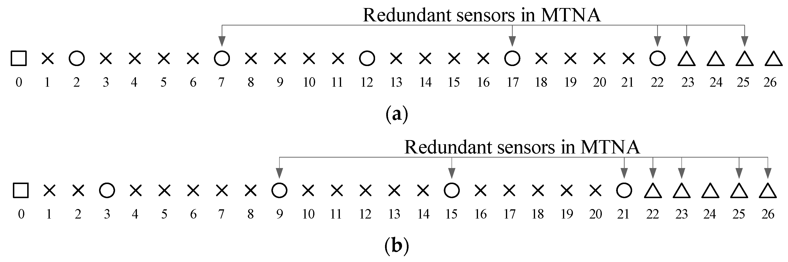
3.1. Introduction of Modified Translational Nested Array (MTNA)

From Reference [25], we know that the sensor positions of translational NA can be expressed as

$$\{\begin{array}{l}{\mathbb{S}}_{1,a_1}=\left\{s_1+a_1|a_1\in \mathbb{Z},s_1=1,2,\cdots ,N_1\right\}\\ {\mathbb{S}}_{2,a_2}=\{s_2\left(N_1+1\right)+a_2|a_2\in Z,s_2=1,2,\cdots ,N_2\}\end{array},$$

(14)

where ${\mathbb{S}}_{1,a_1}$ and ${\mathbb{S}}_{2,a_2}$ represent subarray 1 and subarray 2 of translational NA, respectively. $N_1\in {\mathbb{Z}}^{+}$ and $N_2\in {\mathbb{Z}}^{+}$ respectively denote the sensor number of ${\mathbb{S}}_{1,a_1}$ and ${\mathbb{S}}_{2,a_2}$, while $a_1$ and $a_2$ are the corresponding translation distance. Note that ${\mathbb{Z}}^{+}$ denotes the positive integer set.

It is obvious that the prototype NA is a special case of translational NA with $a_1=a_2=0$. According to Theorem 1 in [25], we know that $a_1$ and $a_2$ should satisfy the following relationships for making the SDCA of translational NA possess the maximum continuous DOFs.

R1: $a_1=a_2=\lfloor \left(\left(N_1+1\right)N_2-2\right)/2\rfloor$.

R2: $a_1=a_2=-\lfloor \left(N_1+1\right)\left(2N_2+1\right)/2\rfloor$.

R3: $a_1=\left(N_1+1\right)N_2+a_2$, $a_2=-\lceil \left(N_1+1\right)/2\rceil$.

R4: $a_1=\left(N_1+1\right)N_2+a_2$, $a_2=-\lfloor \left(\left(N_1+1\right)\left(3N_2+2\right)-2\right)/2\rfloor$.

For the above four cases, $\lfloor \ast \rfloor$ and $\lceil \ast \rceil$ denote the rounding to integer operations, where $\lfloor \ast \rfloor \le \ast$ and $\lceil \ast \rceil \ge \ast$. However, to make the SDCA keep the full continuous characteristic, only the values of $a_1$ and $a_2$ provided in R2 and R3 can be utilized. In addition, corollary 1 in [25] indicates that translational NA structures in R2 and R3 are mirror symmetric about zero point. Therefore, we just need to consider R3 in this paper for the convenience of analysis. Then, Equation (14) can be denoted as:

$$\{\begin{array}{l}{\mathbb{S}}_{1,a}=\left\{s_1+\left(N_1+1\right)N_2+a|s_1=1,2,\cdots ,N_1\right\}\\ {\mathbb{S}}_{2,a}=\left\{s_2\left(N_1+1\right)+a|s_2=1,2,\cdots ,N_2\right\}\end{array},$$

(15)

where $a=-\lceil \left(N_1+1\right)/2\rceil$. When the equivalent received array $\tilde{\mathbb{S}}$ is the union of ${\mathbb{S}}_{1,a}$ and ${\mathbb{S}}_{2,a}$, it is clear from Definition 1 that SDCA can be expressed directly as:

$${\mathbb{V}}_{\mathrm{SDCA}}=\left\{-2\left(M+a\right),-2\left(M+a\right)+1,\cdots ,2\left(M+a\right)-1,2\left(M+a\right)\right\},$$

(16)

where $M=N_1{N}_2+N_1+N_2$. Obviously, SDCA expressed in Equation (16) is completely continuous. From Definition 2 we know that the number of continuous DOFs of SDCA is:

$$L_{\mathrm{c}}=4\left(M+a\right)+1.$$

(17)

Although the translational NA denoted by (15) can generate a continuous SDCA, it cannot be used directly as the received array. The reason has been mentioned in Section 2 that only the equivalent received array $\tilde{\mathbb{S}}$ has a direct connection with SDCA. Specifically, since the elements of $\tilde{\mathbb{S}}$ are obtained by performing the difference operation on those of $\mathbb{S}$, it is obvious that at least one element of $\mathbb{S}$ should be selected as the subtrahend. Nevertheless, observing Equation (15), we can find that all of elements in ${\mathbb{S}}_{1,a}$ and ${\mathbb{S}}_{2,a}$ are always greater than or equal to one. Thus, when $\mathbb{S}$ is the union of ${\mathbb{S}}_{1,a}$ and ${\mathbb{S}}_{2,a}$, $\tilde{\mathbb{S}}$ cannot have the same form as $\mathbb{S}$ regardless of what the index set $\mathbb{N}$ is selected as. In this way, the resulting SDCA can no longer possess the maximum continuous DOFs. To solve the above problem, we modify the translational NA in (15) as follows.

Definition 3.

(MTNA). Let the physical sensor number of subarrays in translational NA are $N_1$ and $N_2$, respectively, then the MTNA can be defined as

$${\mathbb{S}}_{\mathrm{MTNA}}=\left\{0\right\}{\displaystyle \cup }{\mathbb{S}}_{1,a}{\displaystyle \cup }{\mathbb{S}}_{2,a},$$

(18)

where the elements of ${\mathbb{S}}_{MTNA}$ are sorted in ascending order. ${\mathbb{S}}_{1,a}$ and ${\mathbb{S}}_{2,a}$ are defined in Equation (15), and $a=-\lceil \left(N_1+1\right)/2\rceil$.

It is obvious that MTNA is the union of $\left\{0\right\}$, ${\mathbb{S}}_{1,a}$, and ${\mathbb{S}}_{2,a}$. So, the total number of sensors in MTNA is $N=N_1+N_2+1$. In addition, based on the description in Section 2, it is easy to define the index sets as $\mathbb{M}=\left\{2,3,\cdots ,\mathrm{N}\right\}$ and $\mathbb{N}=\left\{1,1,\cdots ,1\right\}$, where $\mathbb{N}$ contains $N_1+N_2$ identical elements, i.e., 1. Combining (18) with its index sets, we have $\tilde{\mathbb{S}}={\mathbb{S}}_{1,a}{\displaystyle \cup }{\mathbb{S}}_{2,a}$, where the corresponding SDCA possesses the maximum continuous DOFs.

Next, we consider an example with $N_1=N_2=3$ to illustrate the above analysis. In this example, sensor positions of subarrays in translational NA can be expressed as ${\mathbb{S}}_{1,-2}=\left\{11,12,13\right\}$ and ${\mathbb{S}}_{2,-2}=\left\{2,6,10\right\}$, respectively. From Definition 3, we can get ${\mathbb{S}}_{\mathrm{MTMA}}=\left\{0,2,6,10,11,12,13\right\}$. Then, letting $\mathbb{M}=\left\{2,3,4,5,6,7\right\}$ and $\mathbb{N}=\left\{1,1,1,1,1,1\right\}$, we have $\tilde{\mathbb{S}}=\left\{2,6,10,11,12,13\right\}$ and ${\mathbb{V}}_{\mathrm{SDCA}}=\{-26,-25,\cdots ,25,26\}$. It is obvious that the resulting SDCA is fully continuous, and the corresponding number of continuous DOFs is equal to 53.

3.2. Redundancy Analysis of MTNA

From the previous subsection, we know that SDCA of MTNA has the maximum continuous DOFs. However, to achieve this goal, the optimal selections of $N_1$ and $N_2$ need to be determined first when we know the total number of sensors $N$. Accordingly, we build the following optimization problem:

$$\underset{N_1,N_2\in {\mathbb{Z}}^{+}}{\max }{L}_{\mathrm{c}}\mathrm{subject}\mathrm{to}:\{\begin{array}{l}N\ge 3\\ N=N_1+N_2+1\end{array}.$$

(19)

Since the specific value of $a$ is related with the parity of $N_1$, we can obtain multiple different solutions of Equation (19) provided below.

S1: If $N=4k$, we have $N_1=2k-1$ and $N_2=2k$. Then, $L_{\mathrm{c}}=16k^2+4k-3$.

S2: If $N=4k+1$, we have $N_1=2k$ and $N_2=2k$, or $N_1=2k-1$ and $N_2=2k+1$. Then, $L_{\mathrm{c}}=16k^2+12k-3$.

S3: If $N=4k+2$, we have $N_1=2k$ and $N_2=2k+1$, or $N_1=2k+1$ and $N_2=2k$. Then, $L_{\mathrm{c}}=16k^2+20k+1$.

S4: If $N=4k+3$, we have $N_1=2k+1$ and $N_2=2k+1$. Then, $L_c=16k^2+28k+9$.

Note that $k$ is a positive integer for the above solutions. Since both S2 and S3 can be divided into two different solutions, it is clear that there exist six different selections about $N_1$ and $N_2$ to maximize $L_{\mathrm{c}}$. Observing $N_1$ and $N_2$ in S1–S4 again, we find that they can also be divided into four different cases from the view of parity property. Accordingly, we derive the following property of MTNA involving redundant sensors.

Property 1.

For MTNA, its redundant sensors can be analyzed under four different combinations of$N_1$and$N_2$, i.e.,

C1: If$N_1\ge 4$and$N_2\ge 4$are even,$\left\{{\mathbb{S}}_{1,a}\left(i\right)\right|i=1,2,\cdots ,N_1/2-1\}$or$\left\{{\mathbb{S}}_{1,a}\left(i\right)\right|i=N_1/2+1,N_1/2+2,\cdots ,N_1-1\}$, and$\left\{{\mathbb{S}}_{2,a}\left(i\right)\right|i=2,3,\cdots ,N_2/2,N_2\}$or$\left\{{\mathbb{S}}_{2,a}\left(i\right)\right|i=N_2/2+1,N_2/2+2,\cdots ,N_2\}$in MTNA are redundant sensors. Then, the total number of redundant sensors is$\left(N_1+N_2-2\right)/2$.

C2: If$N_1\ge 4$is even and$N_2\ge 5$is odd,$\left\{{\mathbb{S}}_{1,a}\left(i\right)\right|i=1,2,\cdots ,N_1/2-1\}$or$\left\{{\mathbb{S}}_{1,a}\left(i\right)\right|i=N_1/2+1,N_1/2+2,\cdots ,N_1-1\}$, and$\left\{{\mathbb{S}}_{2,a}\left(i\right)\right|i=2,3,\cdots ,\left(N_2-1\right)/2,N_2\}$or$\left\{{\mathbb{S}}_{2,a}\left(i\right)\right|i=\left(N_2+3\right)/2,\left(N_2+5\right)/2,\cdots ,N_2\}$in MTNA are redundant sensors. Then, the total number of redundant sensors is$\left(N_1+N_2-3\right)/2$.

C3: If$N_1\ge 3$is odd and$N_2\ge 4$is even,$\left\{{\mathbb{S}}_{1,a}\left(i\right)\right|i=1,2,\cdots ,\left(N_1-1\right)/2\}$or$\left\{{\mathbb{S}}_{1,a}\left(i\right)\right|i=\left(N_1+3\right)/2,\left(N_1+5\right)/2,\cdots ,N_1\}$, and$\left\{{\mathbb{S}}_{2,a}\left(i\right)\right|i=2,3,\cdots ,N_2/2,N_2\}$or$\left\{{\mathbb{S}}_{2,a}\left(i\right)\right|i=N_2/2+1,N_2/2+2,\cdots ,N_2\}$in MTNA are redundant sensors. Then, the total number of redundant sensors is$\left(N_1+N_2-1\right)/2$.

C4: If$N_1\ge 3$and$N_2\ge 5$are odd,$\left\{{\mathbb{S}}_{1,a}\left(i\right)\right|i=1,2,\cdots ,\left(N_1-1\right)/2\}$or$\left\{{\mathbb{S}}_{1,a}\left(i\right)\right|i=\left(N_1+3\right)/2,\left(N_1+5\right)/2,\cdots ,N_1\}$, and$\left\{{\mathbb{S}}_{2,a}\left(i\right)\right|i=2,3,\cdots ,\left(N_2-1\right)/2,N_2\}$or$\left\{{\mathbb{S}}_{2,a}\left(i\right)\right|i=\left(N_2+3\right)/2,\left(N_2+5\right)/2,\cdots ,N_2\}$in MTNA are redundant sensors. Then, the total number of redundant sensors is$\left(N_1+N_2-2\right)/2$.

Proof. 

See Appendix A. □

From Property 1, we can find that although there exist redundant sensors in C1–C4, the number of redundant sensors in C3 is the largest compared to the other three cases, which implies that we can remove more redundant sensors as long as $N_1$ is odd and $N_2$ is even. In order to visually illustrate this interesting phenomenon, Figure 1 depicts two examples, where the total number of sensors is fixed to be 10. According to S3, we can confirm that there exist two different solutions, i.e., $N_1=4$ and $N_2=5$, or $N_1=5$ and $N_2=4$. Then, based on Property 1, if $N_1=4$ and $N_2=5$, the redundant sensors of MTNA as shown in Figure 1a can be expressed as $\left\{23\right\}$ or $\left\{25\right\}$, and $\left\{7,22\right\}$ or $\left\{17,22\right\}$. It is clear that the total number of redundant sensors is 3. Conversely, if $N_1=5$ and $N_2=4$, the redundant sensors of MTNA as shown in Figure 1b can be denoted as $\left\{22,23\right\}$ or $\left\{25,26\right\}$, and $\left\{9,21\right\}$ or $\left\{15,21\right\}$, where the total number of redundant sensors is 4. Note that, the number of rest of sensors for MTNAs shown in Figure 1a,b is 7 and 6, respectively. And, by constructing the time average vectors as described in Section 2, the remaining sensors of MTNAs shown in Figure 1a,b can generate a same SDCA with the maximum continuous DOFs. Hence, for a known total sensor number $N$, when $N_1$ and $N_2$ are respectively odd and even, sensors except for redundant ones in MTNA can generate the SDCA with the largest continuous DOFs.

3.3. The Proposed Novel Nested Arrays (NNAs)

As aforementioned, if $N_1$ is odd and $N_2$ is even, the number of removable sensors in MTNA becomes the largest. Observing C3 mentioned in Property 1, we know that both ${\mathbb{S}}_{1,a}$ and ${\mathbb{S}}_{2,a}$ contain two-part alternative redundant sensors. So, there exist four different combinations for the rest of sensors in ${\mathbb{S}}_{1,a}$ and ${\mathbb{S}}_{2,a}$. Based on this, four kinds of novel nested arrays (NNAs) are defined below.

Definition 4.

(NNAs). Given parameters $N_1\ge 3$ and $N_2\ge 4$, where $N_1$ is odd and $N_2$ is even, then four kinds of NNAs are defined as follows:

(1): If$\left\{{\mathbb{S}}_{1,a}\left(i\right)\right|i=1,2,\cdots ,N_1/2-1\}$and$\left\{{\mathbb{S}}_{2,a}\left(i\right)\right|i=2,3,\cdots ,N_2/2,N_2\}$in${\mathbb{S}}_{\mathrm{MTNA}}$are removed, then the first kind of NNA (i.e., NNA-I) can be expressed as:

$${\mathbb{S}}_{\mathrm{NNA}-\mathrm{I}}=\left\{0\right\}{\displaystyle \cup }{\overline{\mathbb{S}}}_{1,a}{\displaystyle \cup }{\overline{\mathbb{S}}}_{2,a},$$

(20)

where${\overline{\mathbb{S}}}_{1,a}=\left\{{\mathbb{S}}_{1,a}\left(i\right)\right|i=\left(N_1+1\right)/2,\left(N_1+3\right)/2,\cdots ,N_1\}$, ${\overline{\mathbb{S}}}_{2,a}=\left\{{\mathbb{S}}_{2,a}\left(i\right)\right|i=1,N_2/2+1,N_2/2+2,\cdots ,N_2-1\}$.

(2): If$\left\{{\mathbb{S}}_{1,a}\left(i\right)\right|i=1,2,\cdots ,N_1/2-1\}$and$\left\{{\mathbb{S}}_{2,a}\left(i\right)\right|i=N_2/2+1,N_2/2+2,\cdots ,N_2\}$in${\mathbb{S}}_{\mathrm{MTNA}}$are removed, then the second kind of NNA (i.e., NNA-II) can be expressed as:

$${\mathbb{S}}_{\mathrm{NNA}-\mathrm{II}}=\left\{0\right\}{\displaystyle \cup }{\overline{\mathbb{S}}}_{1,a}{\displaystyle \cup }{\overline{\mathbb{S}}}_{2,a},$$

(21)

where${\overline{\mathbb{S}}}_{1,a}=\left\{{\mathbb{S}}_{1,a}\left(i\right)\right|i=\left(N_1+1\right)/2,\left(N_1+3\right)/2,\cdots ,N_1\}$,${\overline{\mathbb{S}}}_{2,a}=\left\{{\mathbb{S}}_{2,a}\left(i\right)\right|i=1,2,\cdots ,N_2/2\}$.

(3): If$\left\{{\mathbb{S}}_{1,a}\left(i\right)\right|i=\left(N_1+3\right)/2,\left(N_1+5\right)/2,\cdots ,N_1\}$and$\left\{{\mathbb{S}}_{2,a}\left(i\right)\right|i=2,3,\cdots ,N_2/2,N_2\}$in${\mathbb{S}}_{\mathrm{MTNA}}$are removed, then the third kind of NNA (i.e., NNA-III) can be expressed as:

$${\mathbb{S}}_{\mathrm{NNA}-\mathrm{III}}=\left\{0\right\}{\displaystyle \cup }{\overline{\mathbb{S}}}_{1,a}{\displaystyle \cup }{\overline{\mathbb{S}}}_{2,a},$$

(22)

where${\overline{\mathbb{S}}}_{1,a}=\{-{\mathbb{S}}_{1,a}\left(i\right)|i=1,2,\cdots ,\left(N_1-1\right)/2\}{\displaystyle \cup }\left\{{\mathbb{S}}_{1,a}\left(\left(N_1+1\right)/2\right)\right\}$,${\overline{\mathbb{S}}}_{2,a}=\left\{{\mathbb{S}}_{2,a}\left(i\right)\right|i=1,N_2/2+1,N_2/2+2,\cdots ,N_2-1\}$.

(4): If$\left\{{\mathbb{S}}_{1,a}\left(i\right)\right|i=\left(N_1+3\right)/2,\left(N_1+5\right)/2,\cdots ,N_1\}$and$\left\{{\mathbb{S}}_{2,a}\left(i\right)\right|i=N_2/2+1,N_2/2+2,\cdots ,N_2\}$in${\mathbb{S}}_{\mathrm{MTNA}}$are removed, then fourth kind of NNA (i.e., NNA-IV) can be expressed as:

$${\mathbb{S}}_{\mathrm{NNA}-\mathrm{III}}=\left\{0\right\}{\displaystyle \cup }{\overline{\mathbb{S}}}_{1,a}{\displaystyle \cup }{\overline{\mathbb{S}}}_{2,a},$$

(23)

where${\overline{\mathbb{S}}}_{1,a}=\{-{\mathbb{S}}_{1,a}\left(i\right)|i=1,2,\cdots ,\left(N_1-1\right)/2\}{\displaystyle \cup }\left\{{\mathbb{S}}_{1,a}\left(\left(N_1+1\right)/2\right)\right\}$,${\overline{\mathbb{S}}}_{2,a}=\left\{{\mathbb{S}}_{2,a}\left(i\right)\right|i=1,2,\cdots ,N_2/2\}$.

It should be noted that, elements of the above NNAs are sorted in ascending order of their respective absolute values. Meanwhile, different index sets $\mathbb{M}$ and $\mathbb{N}$ corresponding to the above four kinds of NNAs are defined as follows.

Definition 5.

(Index Sets). For NNA-I and NNA-II, the index sets are collectively defined as:

$$\{\begin{array}{c}{\mathbb{M}}_1={\overline{\mathbb{M}}}_{1,1}{\displaystyle \cup }{\overline{\mathbb{M}}}_{1,2}{\displaystyle \cup }{\overline{\mathbb{M}}}_{1,3}\\ {\mathbb{N}}_1={\overline{\mathbb{N}}}_{1,1}{\displaystyle \cup }{\overline{\mathbb{N}}}_{1,2}{\displaystyle \cup }{\overline{\mathbb{N}}}_{1,3}\end{array},$$

(24)

where

$$\begin{array}{l}{\overline{\mathbb{M}}}_{1,1}=\underset{\left(N_1+N_2+1\right)/2}{\underbrace{\left\{1,1,\cdots ,1\right\}}},\\ {\overline{\mathbb{M}}}_{1,2}=\underset{\left(N_1+1\right)/2}{\underbrace{\left\{2,2,\cdots ,2\right\}}},\\ {\overline{\mathbb{M}}}_{1,3}=\left\{3,4,\cdots ,N_2/2+1\right\},\\ {\overline{\mathbb{N}}}_{1,1}=\left\{2,3,\cdots ,\left(N_1+N_2+3\right)/2\right\},\\ {\overline{\mathbb{N}}}_{1,2}=\left\{N_2/2+2,N_2/2+3,\cdots ,\left(N_1+N_2+3\right)/2\right\},\\ {\overline{\mathbb{N}}}_{1,3}=\underset{N_2/2-1}{\underbrace{\left\{N_2/2+2,N_2/2+2,\cdots ,N_2/2+2\right\}}}.\end{array}$$

For NNA-III and NNA-IV, the index sets are collectively defined as:

$$\{\begin{array}{l}{\mathbb{M}}_2={\overline{\mathbb{M}}}_{2,1}{\displaystyle \cup }{\overline{\mathbb{M}}}_{2,2}{\displaystyle \cup }{\overline{\mathbb{M}}}_{2,3}{\displaystyle \cup }{\overline{\mathbb{M}}}_{2,4}\\ {\mathbb{N}}_2={\overline{\mathbb{N}}}_{2,1}{\displaystyle \cup }{\overline{\mathbb{N}}}_{2,2}{\displaystyle \cup }{\overline{\mathbb{N}}}_{2,3}{\displaystyle \cup }{\overline{\mathbb{N}}}_{2,4}\end{array},$$

(25)

where

$$\begin{array}{l}{\overline{\mathbb{M}}}_{2,1}=\underset{N_2/2+1}{\underbrace{\left\{1,1,\cdots ,1\right\}}},\\ {\overline{\mathbb{M}}}_{2,2}=\left\{2,3,\cdots ,N_2/2+1\right\},\\ {\overline{\mathbb{M}}}_{2,3}={\overline{\mathbb{M}}}_{2,4}=\left\{N_2/2+2,N_2/2+3,\cdots ,\left(N_1+N_2+1\right)/2\right\},\\ {\overline{\mathbb{N}}}_{2,1}=\left\{2,3,\cdots ,N_2/2+1,\left(N_1+N_2+3\right)/2\right\},\\ {\overline{\mathbb{N}}}_{2,2}=\underset{N_2/2}{\underbrace{\left\{\left(N_1+N_2+3\right)/2,\left(N_1+N_2+3\right)/2,\cdots ,\left(N_1+N_2+3\right)/2\right\}}},\\ {\overline{\mathbb{N}}}_{2,3}=\underset{\left(N_1-1\right)/2}{\underbrace{\left\{1,1,\cdots ,1\right\}}},\\ {\overline{\mathbb{N}}}_{2,4}=\underset{\left(N_1-1\right)/2}{\underbrace{\left\{2,2,\cdots ,2\right\}}}.\end{array}$$

Apparently, combining NNAs with their respective index sets, according to the construction principle in Definition 1, we can construct the specific time average vectors so as to obtain the equivalent received array $\tilde{\mathbb{S}}$, and then the satisfying SDCA with maximum continuous DOFs can be obtained. Nevertheless, although NNAs and index sets are already given in Definitions 4 and 5, the relationship among $N_1$, $N_2$, and total number of sensors of NNAs is still indistinct. Hence, before using NNAs for DOA estimation, we need to address this problem first. Note that, it is apparent from Definition 4 that the sensor number of NNAs is $\overline{N}=\left(N_1+N_2+3\right)/2$. From Equation (17), we know that the number of continuous DOFs of SDCA is $L_{\mathrm{c}}=4\left(M+a\right)+1$, where $M=N_1{N}_2+N_1+N_2$ and $a=-\lceil \left(N_1+1\right)/2\rceil$. Hence, the optimization problem can be constructed as follows:

$$\underset{\overline{N},N_1,N_2\in {\mathbb{Z}}^{+}}{\max }{L}_{\mathrm{c}}\mathrm{subject}\mathrm{to}:\{\begin{array}{l}{N}_1\ge 3\mathrm{is}\mathrm{odd}\\ N_2\ge 4\mathrm{is}\mathrm{even}\\ \overline{N}=\left(N_1+N_2+3\right)/2\end{array}.$$

(26)

Combining C3 in Property 1 with Equation (26), it is easy to get the relationship among $\overline{N}$, $N_1$, $N_2$, as well as $L_{\mathrm{c}}$, which is as shown in

Table 1. Relationship among $\overline{N}$, $N_1$, $N_2$, and $L_{\mathrm{c}}$ for the proposed four kinds of novel nested arrays (NNAs).

$\overline{\mathit{N}}$	${\mathit{N}}_{\mathbf{1}}$	${\mathit{N}}_{\mathbf{2}}$	${\mathit{L}}_{\mathbf{c}}$
$\overline{N}\ge 5$ is odd	$\overline{N}-2$	$\overline{N}-1$	4${\overline{N}}^2-6\overline{N}-1$
$\overline{N}\ge 6$ is even	$\overline{N}-1$	$\overline{N}-2$	4${\overline{N}}^2-6\overline{N}-3$

.

Then, according to Table 1 and Definition 4, physical apertures of the proposed four kinds of NNAs can be summarized as follows.

Property  2.

For NNA-I and NNA-II with$\overline{N}$sensors, their physical apertures are identical and can be expressed as:

$$L_{\mathrm{PA}}=\{\begin{array}{l}{\overline{N}}^2-3\overline{N}/2-1/2,\mathrm{if}\overline{N}\ge 5\mathrm{is}\mathrm{odd}\\ {\overline{N}}^2-3\overline{N}/2-1,\mathrm{if}\overline{N}\ge 6\mathrm{is}\mathrm{even}\end{array}.$$

(27)

While for NNA-III and NNA-IV with$\overline{N}$sensors, their physical apertures are also identical and can be expressed as:

$$L_{\mathrm{PA}}=\{\begin{array}{l}2{\overline{N}}^2-4\overline{N}+1,\mathrm{if}\overline{N}\ge 5\mathrm{is}\mathrm{odd}\\ 2{\overline{N}}^2-4\overline{N}-1,\mathrm{if}\overline{N}\ge 6\mathrm{is}\mathrm{even}\end{array}.$$

(28)

Proof. 

See Appendix B. □

It is obvious from Property 2 that NNA-III and NNA-IV possess larger physical aperture than NNA-I and NNA-II for the same sensor number, which means that the former can realize better DOA estimation performance than the latter.

Next, to illustrate the exploitation of the proposed NNAs and index sets more clearly, two examples of NNA-I and NNA-IV are provided as shown in Figure 2. Let $\overline{N}$ be 10, then the optimal $N_1$ and $N_2$ are 9 and 8, respectively. According to Definition 4, the sensor position sets of NNA-I and NNA-IV can be given as ${\mathbb{S}}_{\mathrm{NNA}-\mathrm{I}}=\left\{0,5,45,55,65,80,81,82,83,84\right\}$ and ${\mathbb{S}}_{\mathrm{NNA}-\mathrm{IV}}=\{0,5,15,25,35,-76,-77,-78,-79,80\}$, respectively. It is evident that physical apertures of NNA-I and NNA-IV are respectively equal to 84 and 159. Shown in Figure 2a is the physical structure of NNA-I, while Figure 2b shows the physical structure of NNA-IV. Besides, from Definition 5, we can determine their respective index sets as ${\mathbb{M}}_1=\left\{1,1,1,1,1,1,1,1,1,2,2,2,2,2,3,4,5\right\}$, ${\mathbb{N}}_1=\{2,3,4,5,6,7,8,9,10,6,7,8,9,10,6,6,6\}$, ${\mathbb{M}}_2=\left\{1,1,1,1,1,2,3,4,5,6,7,8,9,6,7,8,9\right\}$, and ${\mathbb{N}}_2=\left\{2,3,4,5,10,10,10,10,10,1,1,1,1,2,2,2,2\right\}$. As shown in Figure 2c, we then obtain the equivalent received arrays of NNA-I and NNA-IV, which are identical and can be expressed as $\tilde{\mathbb{S}}=\left\{5,15,25,35,45,55,65,75,76,\cdots ,84\right\}$. Finally, according to Equation (12), we can easily obtain this fully continuous SDCA. It is obvious from Figure 2d that the number of continuous DOFs of SDCA is equal to 337. However, in both of these examples, physical aperture of NNA-IV is larger than that of NNA-I. Thus, we can infer that NNA-IV has better DOA estimation performance than NNA-I.

4. Simulation Results

In this section, we conduct several simulation experiments to demonstrate the superiority of the proposed NNAs. It should be noted that the unit inter-element spacing in all of the experiments is set to be half a wavelength and the VCAM method is used for DOA estimation.

4.1. Continuous Degrees of Freedom (DOFs) and Physical Aperture

In the first experiment, comparisons about continuous DOFs and physical aperture are carried out to show the superiority of the proposed arrays. According to the analysis in Section 3, we know that SDCA of the proposed four kinds of NNAs are identical. Moreover, it is obvious from Property 2 that NNA-I and NNA-II have the same physical aperture, and NNA-III and NNA-IV have this property as well. Thus, we only select NNA-I and NNA-IV in this experiment. In addition, state-of-the-art sparse arrays including TCPA [16,17], DsNA [24], and INAwSDCA-I [25] are chosen to be the comparison arrays here.

If we let the number of physical sensors vary from 5 to 30, then the comparisons of continuous DOFs and the physical aperture are depicted in Figure 3a,b, respectively. Since NNA-I and NNA-IV possess the same SDCA, their corresponding number of continuous DOFs will be identical. Therefore, we mark NNA-I and NNA-IV as NNAs in Figure 3a to distinguish them from other sparse arrays. Clearly, as can be seen from Figure 3a, the number of continuous DOFs of NNAs is significantly higher than that of other sparse arrays. From Figure 3b, we observe that the physical aperture of NNA-IV is the largest among all arrays. In addition, the physical aperture of NNA-I is augmented as well, especially for the situation with a large number of sensors. The above results mean that the proposed arrays can exhibit better DOA estimation performance than the other arrays.

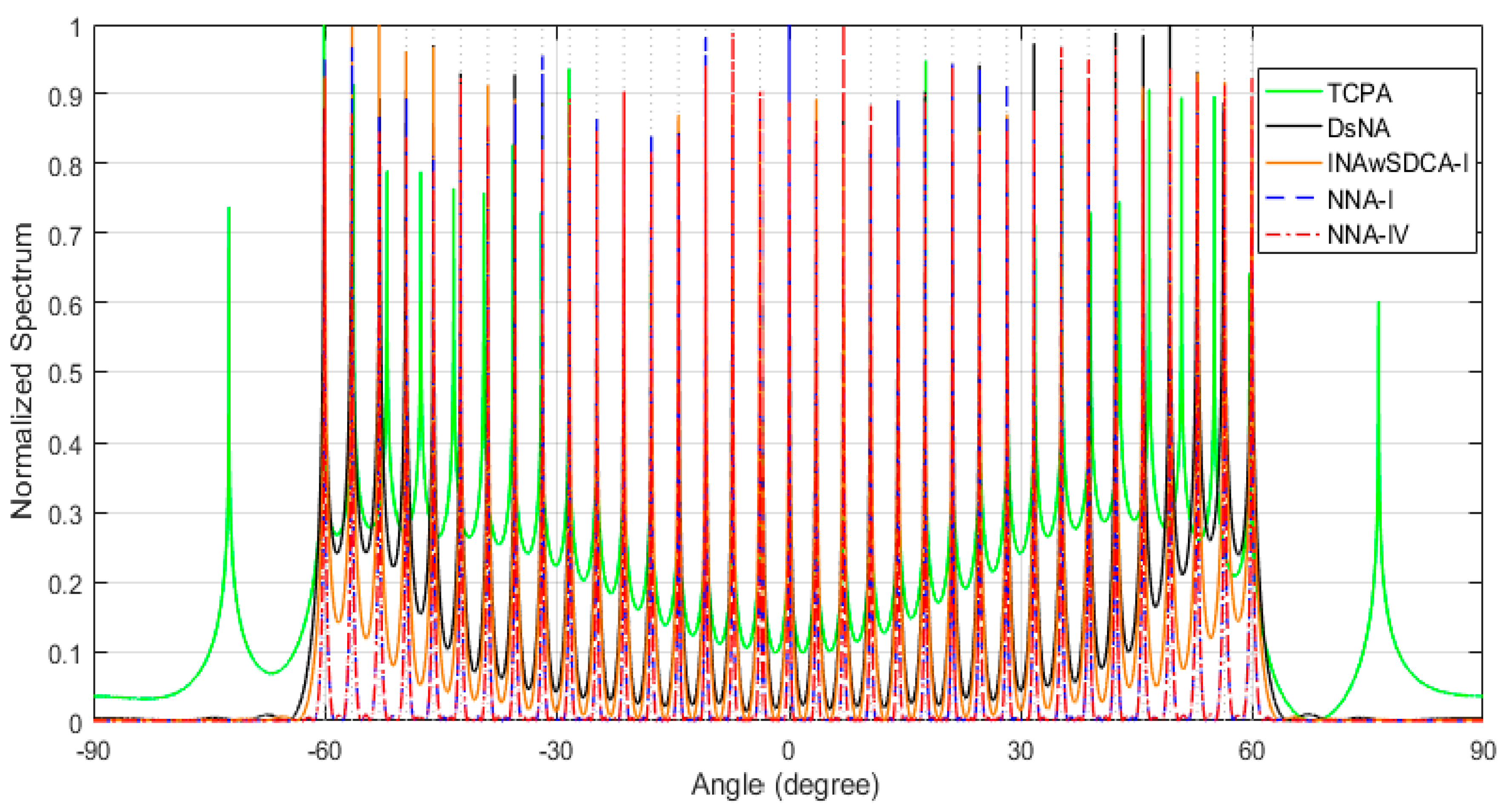
4.2. Normalized Spectra

To illustrate the DOA estimation capability of the proposed arrays, normalized spectra of NNA-I, NNA-IV, and comparison arrays are presented in this subsection. For the second experiment, the number of sensors is set to be 10. Then, sensor positions of TCPA, DsNA, and INAwSDCA-I are, respectively, specified as ${\mathbb{S}}_{\mathrm{TCPA}}=\left\{0,4,5,8,10,12,16,25,30,35\right\}$, ${\mathbb{S}}_{\mathrm{DsNA}}=\left\{0,3,5,7,8,17,26,35,44,53\right\}$, ${\mathbb{S}}_{\mathrm{INAwSDCA}-\mathrm{I}}=\left\{0\right\}{\displaystyle \cup }\left\{-38,-26,-19,-16,18,20,44\right\}{\displaystyle \cup }\left\{17,32\right\}$. The sensor positions of NNA-I and NNA-IV, as well as their respective index sets are given in the examples of Figure 2. When we use the VCAM method for DOA estimation, the maximum number of identifiable sources of the above arrays is equal to 35 (TCPA), 53 (DsNA), 64 (INAwSDCA-I), and 168 (NNA-I and NNA-IV), respectively. Accordingly, consider $K=35$ signals that are uniformly distributed in the range of $\left[-{60}^{°},{60}^{°}\right]$ impinging on the arrays with their corresponding small frequency offsets being evenly distributed between $-3\mathrm{MHz}$ and $3\mathrm{MHz}$. SNR is set to be 0 dB and $N_{\mathrm{s}}=N_{\mathrm{p}}=800$. In addition, the search interval in VCAM method is fixed to be ${0.01}^{°}$.

We can then obtain all the normalized spectra, as shown in Figure 4. As can be seen from Figure 4, TCPA cannot identify all the DOAs correctly. Although the rest of arrays can estimate all the DOAs effectively, it is visible that the normalized spectra of NNA-I and NNA-IV are sharper than those of DsNA and INAwSDCA-I. The reason is that the maximum number of identifiable sources of NNA-I and NNA-IV is identical and significantly larger than that of other arrays, which is even much larger than the number of incident signals set in this subsection. As a result, we know that the proposed arrays possess superior DOA estimation capability in comparison with the other arrays.

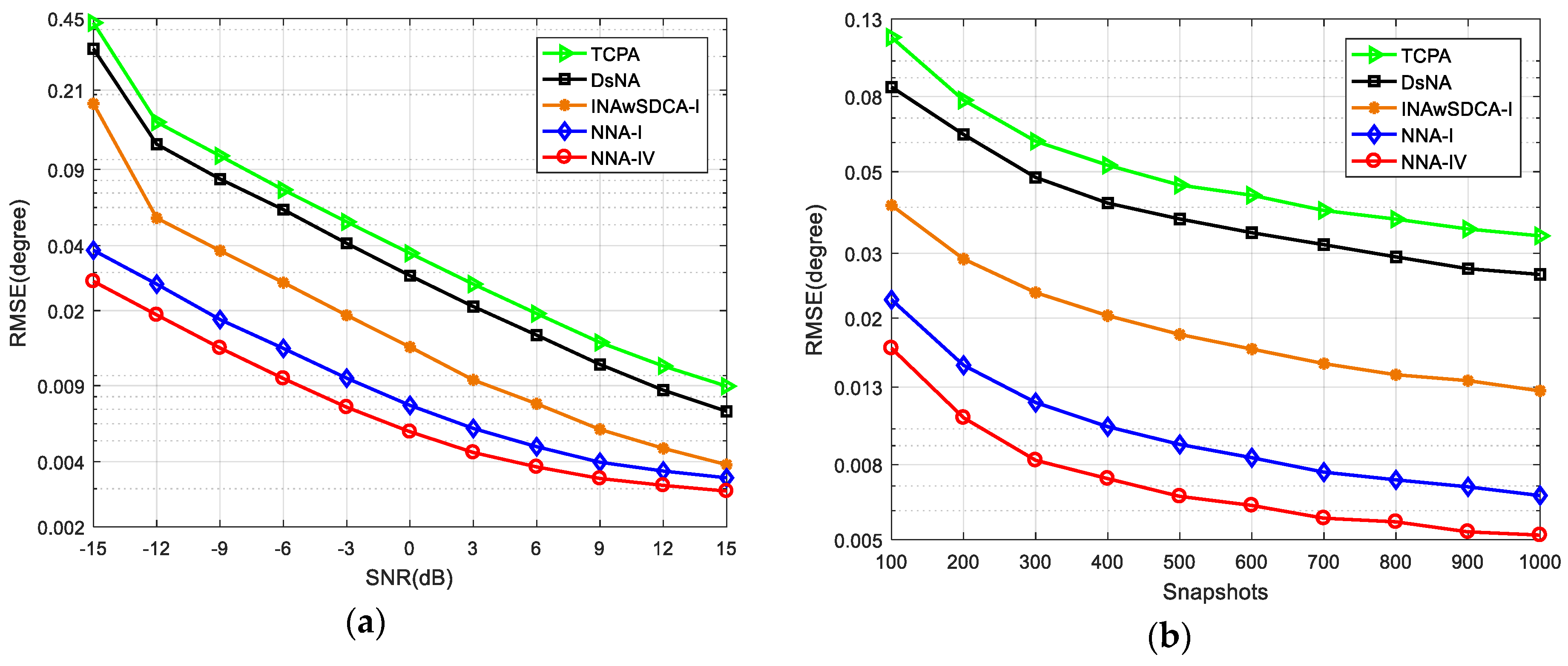
4.3. Root-Mean-Squared Error (RMSE)

In the third experiment, comparisons about root-mean-squared error (RMSE) of the estimated DOAs are conducted with 500 Monte Carlo trials to further demonstrate the superiority of the proposed arrays. Here, the RMSE is defined as:

$$\mathrm{RMSE}=\sqrt{\frac{1}{500K}{\displaystyle \sum }_{q=1}^{500}{\displaystyle \sum }_{k=1}^K{({\hat{\theta }}_{k,q}-{\theta }_k)}^2},$$

(29)

where ${\hat{\theta }}_{k,q}$ represents the estimated DOA of ${\theta }_k$ in the $q$-th trial.

First, we assume that $K=18$ signals with uniform distribution between $-{60}^{°}$ and ${60}^{°}$ impinge on the received arrays. Except for SNR, $N_{\mathrm{s}}$, and $N_{\mathrm{p}}$, the other parameters are set the same as those in the previous subsection. As such, physical apertures of all the arrays with 10 sensors satisfy $35\left(\mathrm{TCPA}\right)<53\left(\mathrm{DsNA}\right)<82\left(\mathrm{INAwSDCA}-\mathrm{I}\right)<84\left(\mathrm{NNA}-\mathrm{I}\right)<159\left(\mathrm{NNA}-\mathrm{IV}\right)$. Likewise, continuous DOFs of SDCAs for all the arrays satisfy $71\left(\mathrm{TCPA}\right)<107\left(\mathrm{DsNA}\right)<129\left(\mathrm{INAwSDCA}-\mathrm{I}\right)<337\left(\mathrm{NNA}-\mathrm{I}\right)=337\left(\mathrm{NNA}-\mathrm{IV}\right)$.

Figure 5a shows the RMSE curves as a function of SNR, where $N_{\mathrm{s}}=N_{\mathrm{p}}=800$, while Figure 5b depicts the RMSE curves as a function of snapshots, where SNR is fixed to be 0dB and $N_{\mathrm{s}}=N_{\mathrm{p}}$. From Figure 5, we observe that with the increase of SNR and snapshots, RMSE results for all the arrays are decreased. In addition, it is obvious that RMSE results of NNA-I and NNA-IV are smaller than those of comparison arrays. This is because that compared with TCPA, DsNA, and INAwSDCA-I, both NNA-I and NNA-IV not only possess larger physical apertures but also can generate the SDCA with higher continuous DOFs. Owing to the fact that physical aperture of NNA-IV is larger than that of NNA-I, NNA-IV possesses the best DOA estimation accuracy. Moreover, the above RMSE results show the superiority of the proposed arrays.

Next, let $\mathrm{SNR}=0\mathrm{dB}$, $N_{\mathrm{s}}=N_{\mathrm{p}}=800$, the number of signals vary from 5 to 100, and keep the remaining simulation parameters unchanged. Then, we can draw the RMSE curves versus the number of signals as shown in Figure 6.

It is clear from Figure 6 that, with the increase of source number, RMSE results of NNA-IV are always the smallest, followed by NNA-I, INAwSDCA-I, and DsNA, while TCPA always possess the largest RMSE results. The reasons have been given in the description about Figure 5. In addition, from the previous subsection we know that the maximum number of identifiable signals for TCPA, DsNA, and INAwSDCA-I is 35, 53, and 64, respectively, which means that these comparison arrays may not be able to correctly estimate the DOAs of all incident signals when the actual number of signals is close to their respective maximum number of identifiable signals due to the existence of noise or other factors. Obviously, it can be seen from Figure 6 that the RMSE results of these comparison arrays increase sharply when their corresponding number of signals is equal to 35, 45, and 50, while that of the proposed arrays do not fluctuate much. Thus, according to these simulation results, we can draw the conclusion that the proposed arrays own much superior DOA estimation performance compared with other sparse arrays.

5. Conclusions

In this paper, four kinds of NNAs have been proposed through the joint exploitation of spatial and temporal information. In addition, different index sets have also been defined so as to construct the desirable time average vectors to generate the SDCA with increased continuous DOFs. The property analysis has showed that the four proposed kinds of arrays not only have increased physical apertures but also can generate the SDCA with significantly enhanced continuous DOFs. As a result, the proposed arrays possess better DOA estimation capability. At last, simulation results have demonstrated the superiority and effectiveness of the proposed arrays.

References

- Merrill, I.S. Introduction to Radar Systems, 3rd ed.; McGraw-Hill: New York, NY, USA, 2001. [Google Scholar]
- Chen, P.; Cao, Z.; Chen, Z.; Yu, C. Sparse DOD/DOA estimation in a bistatic MIMO radar with mutual coupling effect. Electronics 2018, 7, 341. [Google Scholar] [CrossRef]
- Krim, H.; Viberg, M. Two decades of array signal processing research: The parametric approach. IEEE Signal Process. Mag. 1996, 13, 67–94. [Google Scholar] [CrossRef]
- Wan, L.; Han, G.; Shu, L.; Chan, S.; Zhu, T. The application of DOA estimation approach in patient tracking systems with high patient density. IEEE Trans. Ind. Informat. 2016, 12, 2353–2364. [Google Scholar] [CrossRef]
- Han, M.; Dou, W. Atomic norm-based DOA estimation with dual-polarized radar. Electronics 2019, 8, 1056. [Google Scholar] [CrossRef]
- Schmidt, R. Multiple emitter location and signal parameter estimation. IEEE Trans. Antennas Propag. 1986, 34, 276–280. [Google Scholar] [CrossRef]
- Roy, R.; Kailath, T. ESPRIT-estimation of signal parameters via rotational invariance techniques. IEEE Trans. Acoust. Speech Signal Process. 1989, 37, 984–995. [Google Scholar] [CrossRef]
- Pal, P.; Vaidyanathan, P.P. Nested arrays: A novel approach to array processing with enhanced degrees of freedom. IEEE Trans. Signal Process. 2010, 58, 4167–4181. [Google Scholar] [CrossRef]
- Boccardi, F.; Heath, R.W.; Lozano, A.; Marzetta, T.L.; Popovski, P. Five disruptive technology directions for 5G. IEEE Commun. Mag. 2014, 52, 74–80. [Google Scholar] [CrossRef]
- Pal, P.; Vaidyanathan, P.P. Coprime Sampling and the Music Algorithm. In Proceedings of the 14th IEEE DSP/SPE Workshop, Sedona, AZ, USA, 4–7 January 2011; pp. 289–294. [Google Scholar]
- Moffet, A. Minimum-redundancy linear arrays. IEEE Trans. Antennas Propag. 1968, 16, 172–175. [Google Scholar] [CrossRef]
- Vertatschitsch, E.; Haykin, S. Nonredundant arrays. Proc. IEEE 1986, 74, 217. [Google Scholar] [CrossRef]
- Vaidyanathan, P.P.; Pal, P. Sparse sensing with co-prime samplers and arrays. IEEE Trans. Signal Process. 2011, 59, 573–586. [Google Scholar] [CrossRef]
- Qin, S.; Zhang, Y.D.; Amin, M.G. Generalized coprime array configurations for direction-of-arrival estimation. IEEE Trans. Signal Process. 2015, 63, 1377–1390. [Google Scholar] [CrossRef]
- Wang, W.J.; Ren, S.W.; Chen, Z.M. Unified coprime array with multi-period subarrays for direction-of-arrival estimation. Digit. Signal Process. 2018, 74, 30–42. [Google Scholar] [CrossRef]
- Raza, A.; Liu, W.; Shen, Q. Thinned coprime arrays for DOA estimation. In Proceedings of the European Signal Proceeding Conference, Kos, Greece, 28 August–2 September 2017; pp. 395–399. [Google Scholar]
- Raza, A.; Liu, W.; Shen, Q. Thinned coprime array for second-order difference co-array generation with reduced mutual coupling. IEEE Trans. Signal Process. 2019, 67, 2052–2065. [Google Scholar] [CrossRef]
- Yang, M.; Sun, L.; Yuan, X.; Chen, B. Improved nested array with hole-free DCA and more degrees of freedom. Electron. Lett. 2016, 52, 2068–2070. [Google Scholar] [CrossRef]
- Liu, J.Y.; Zhang, Y.M.; Lu, Y.L.; Ren, S.W.; Cao, S. Augmented nested arrays with enhanced DOF and reduced mutual coupling. IEEE Trans. Signal Process. 2017, 65, 5549–5563. [Google Scholar] [CrossRef]
- Zhang, Y.K.; Xu, H.Y.; Zong, R.; Ba, B.; Wang, D.M. A novel high degree of freedom sparse array with displaced multistage cascade subarrays. Digit. Signal Process. 2019, 90, 36–45. [Google Scholar] [CrossRef]
- Liu, C.L.; Vaidyanathan, P.P. Composite singer arrays with hole-free coarrays and enhanced robustness. In Proceedings of the IEEE International Conference on Acoustics, Speech Signal Processing (ICASSP), Brighton, UK, 12–17 May 2019; pp. 4120–4124. [Google Scholar]
- Wang, X.H.; Chen, Z.H.; Ren, S.W.; Cao, S. DOA estimation based on the difference and sum coarray for coprime arrays. Digit. Signal Process. 2017, 69, 22–31. [Google Scholar] [CrossRef]
- Iwazaki, S.; Ichige, K. Underdetermined direction of arrival estimation by sum and difference composite co-array. In Proceedings of the 25th IEEE International Conference on Electronics Circuits and Systems, Bordeaux, France, 9–12 December 2018; pp. 669–672. [Google Scholar]
- Chen, Z.; Ding, Y.; Ren, S.; Chen, Z. A novel nested configuration based on the difference and sum co-array concept. Sensors 2018, 18, 2988. [Google Scholar] [CrossRef]
- Si, W.J.; Peng, Z.L.; Hou, C.B.; Zeng, F.H. Improved nested arrays with sum-difference coarray for DOA estimation. IEEE Sens. J. 2019, 19, 6986–6997. [Google Scholar] [CrossRef]
- Si, W.J.; Zeng, F.H.; Zhang, C.J.; Peng, Z.L. Improved coprime arrays with reduced mutual coupling based on the concept of difference and sum coarray. IEEE Access 2019, 7, 66251–66262. [Google Scholar] [CrossRef]
- Shan, Z.; Yum, T.S.P. A conjugate augmented approach to direction-of-arrival estimation. IEEE Trans. Signal Process. 2005, 53, 4104–4109. [Google Scholar] [CrossRef]
- Mahafza, B.R. Introduction to Radar Analysis; Chapman and Hall/CRC: New York, NY, USA, 2017. [Google Scholar]
- Liu, C.L.; Vaidyanathan, P.P. Cramér–rao bounds for coprime and other sparse arrays, which find more sources than sensors. Digit. Signal Process. 2017, 61, 43–61. [Google Scholar] [CrossRef]
- Wang, M.Z.; Nehorai, A. Coarrays, MUSIC, and the cramér–rao bound. IEEE Trans. Signal Process. 2017, 65, 933–946. [Google Scholar] [CrossRef]
- Shan, T.-J..; Wax, M.; Kailath, T. On spatial smoothing for direction-of-arrival estimation of coherent signals. IEEE Trans. Acoust. Speech Signal Process. 1985, 33, 806–811. [Google Scholar] [CrossRef]
- Liu, C.L.; Vaidyanathan, P.P. Remarks on the spatial smoothing step in coarray MUSIC. IEEE Signal Process. Lett. 2015, 22, 1438–1442. [Google Scholar] [CrossRef]