Statistical Modeling of PPP-RTK Derived Ionospheric Residuals for Improved ARAIM MHSS Protection Level Calculation

Abstract

Ensuring Global Navigation Satellite System (GNSS) integrity, which provides operational reliability via fault detection, is important for safety-critical applications using high-precision techniques like Precise Point Positioning (PPP) and Real-Time Kinematic (RTK). Ionospheric errors, from atmospheric free electrons, challenge this integrity by introducing variable uncertainties into positioning solutions. This study investigates how ionospheric error modeling spatial resolution impacts protection level (PL) calculations, a metric defining positioning error bounds with high confidence. A comparative evaluation was conducted in low-latitude (Guangdong) and mid-latitude (Shandong) regions, contrasting large-scale with small-scale grid-based ionospheric models from regional GNSS networks. Experimental results show small-scale grids improve characterization of localized ionospheric variability, reducing ionospheric residual standard deviation by approximately 30% and enhancing PL precision. Large-scale grids show limitations, especially in active low-latitude conditions, leading to conservative PLs that reduce system availability and increase missed fault detection risks. A user-side PL computation framework incorporating this high-resolution ionospheric residual uncertainty improved system availability to 94.7% and lowered misleading and hazardous outcomes by over 80%. This research indicates that refined, high-resolution ionospheric modeling improves operational reliability and safety for high-integrity GNSS applications, particularly under diverse and challenging ionospheric conditions.

1. Introduction

With the rapid development of Global Navigation Satellite System (GNSS) technology, its applications are becoming increasingly widespread in various fields including, but not limited to, geodesy, traffic navigation, and precision agriculture [1]. The performance of GNSSs not only depends on positioning accuracy but also on system integrity—the ability to detect and alert for potential system faults and performance degradation in a timely manner. Integrity, as an important indicator of navigation service performance, is crucial for ensuring user safety [2,3]. This imperative is particularly pronounced in high-precision applications such as Precise Point Positioning (PPP) and Real-Time Kinematic (RTK). However, the reliability of these high-precision GNSS applications can be significantly compromised in challenging environments. For instance, in complex urban scenes, GNSS signals are often obstructed or reflected by high-rise buildings, leading to multipath, non-line-of-sight issues, and gross errors that degrade positioning accuracy and reliability, necessitating robust mitigation strategies such as advanced filtering or optimization models [4]. Similarly, when GNSS signals are temporarily lost or interfered with, traditional integrated navigation systems may degenerate, leading to a rapid decrease in navigation accuracy unless effective compensation methods, such as predictive modeling for pseudo-GNSS signals, are employed [5]. These challenges are not limited to ground-based applications; for instance, Unmanned Aerial Vehicles (UAVs) operating in mountainous terrain face issues in maintaining flight precision [6], and UAV operations in urban environments necessitate careful risk assessment due to signal complexities and potential ground impact [7]. In light of these vulnerabilities, precise error modeling and uncertainty quantification, especially for dominant error sources like the ionosphere, become key factors not only in improving positioning accuracy but also in ensuring the overall reliability and integrity of the system [8,9,10].

GNSS signals are affected by free electrons as they pass through the ionosphere, causing signal path bending and velocity changes, which in turn affect the accuracy of positioning results [11]. As a critical component of the near-Earth space environment, the ionosphere primarily influences GNSS signals by reducing positioning accuracy and, in severe cases, limiting service availability. Ionospheric errors constitute one of the major error sources in GNSS measurements, with their impact varying significantly over time and space, capable of causing positioning errors ranging from a few meters to over a hundred meters [12,13,14]. The spatiotemporal variations in ionospheric total electron content (TEC) fluctuations across China have been comprehensively characterized using the GPS-based Rate of TEC Index, revealing strong latitude- and season-dependent behaviors [15]. Although classical broadcast ionospheric models, such as the Klobuchar model, are widely used in GNSS applications, their ability to capture temporal variations is limited, especially under dynamic or nighttime conditions. To overcome these shortcomings, sophisticated models employing time-series forecasting methods have been proposed, such as the Sophisticated Klobuchar Model (SKM), which demonstrated improved vertical total electron content prediction performance over China [16]. These studies highlight the necessity of developing more dynamic and region-adaptive ionospheric error models to enhance GNSS integrity performance.

In undifferenced and uncombined Precise Point Positioning-Real-Time Kinematic (PPP-RTK) technology, accurate estimation and correction of ionospheric errors are crucial for improving positioning accuracy and integrity. The key to ionospheric error modeling lies in determining the TEC, which is proportional to the total number of electrons along the signal propagation path and inversely proportional to the square of the carrier frequency [17,18,19]. By studying the temporal and spatial variation characteristics of the ionosphere, one can better understand the inherent changes, which helps mitigate ionospheric errors and improve navigation positioning accuracy.

Ionospheric error uncertainty quantification is vital for assessing and improving GNSS positioning accuracy. Ionospheric error uncertainty not only affects positioning accuracy but also directly relates to the concept of protection level (PL) in GNSS integrity [20]. PL is an important parameter in GNSS integrity, defining the maximum error threshold that a user receiver can detect and alarm, at a specified confidence level.

In integrity assessment, ionospheric error modeling and quantification are crucial for determining the PL. The dynamic changes and uncertainty of the ionosphere require GNSSs to provide timely error alerts to ensure user safety [21]. However, existing integrity frameworks, such as Advanced Receiver Autonomous Integrity Monitoring (ARAIM), often face challenges in effectively incorporating highly dynamic and localized ionospheric error models at the user level. Standard ARAIM implementations may rely on pre-defined, conservative ionospheric threat models or simplified error parameters that may not adequately capture real-time, high-frequency ionospheric variations, particularly in active regions [22]. User equipment typically has limited computational capacity and access to the dense network data required for sophisticated regional ionospheric modeling. This makes it difficult for standalone users to generate and utilize precise, real-time ionospheric corrections and their associated uncertainties for PL computation. Consequently, there is often a trade-off between the conservatism of the ionospheric error bounds and the risk of unmodeled ionospheric effects. While some approaches treat ionospheric errors as constants in PL calculations, this simplification fails to account for the complex temporal and spatial characteristics of the ionosphere, leading to potential integrity vulnerabilities [23]. This study aims to comprehensively analyze the integrity of undifferenced and uncombined PPP-RTK GNSSs enhanced by sophisticated ionospheric error modeling, with a particular focus on developing and evaluating methods for quantifying ionospheric error uncertainty. A key aspect of our approach is the derivation of ionospheric integrity parameters from a server-side perspective, leveraging regional network data, and proposing an effective way these parameters can inform user-side PL calculations. To address the specific requirements of high-integrity applications, this research systematically investigates the spatiotemporal characteristics of the ionosphere and their impact on positioning errors, considering various grid sizes of ionospheric networks at different scales. In terms of error modeling, a server-side product evaluation framework for ionospheric models at these varying scales is constructed using empirical data. By quantitatively analyzing the spatiotemporal correlation of ionospheric delays, a more precise error model is established. Regarding integrity computation, an innovative method is proposed for the efficient transmission of server-side integrity parameters to the user side, thereby providing a more reliable reference for the calculation of PLs. This research effectively addresses challenges encountered by traditional algorithms in handling ionospheric error uncertainty and integrity assessment. The main contributions of this paper can be summarized as follows:

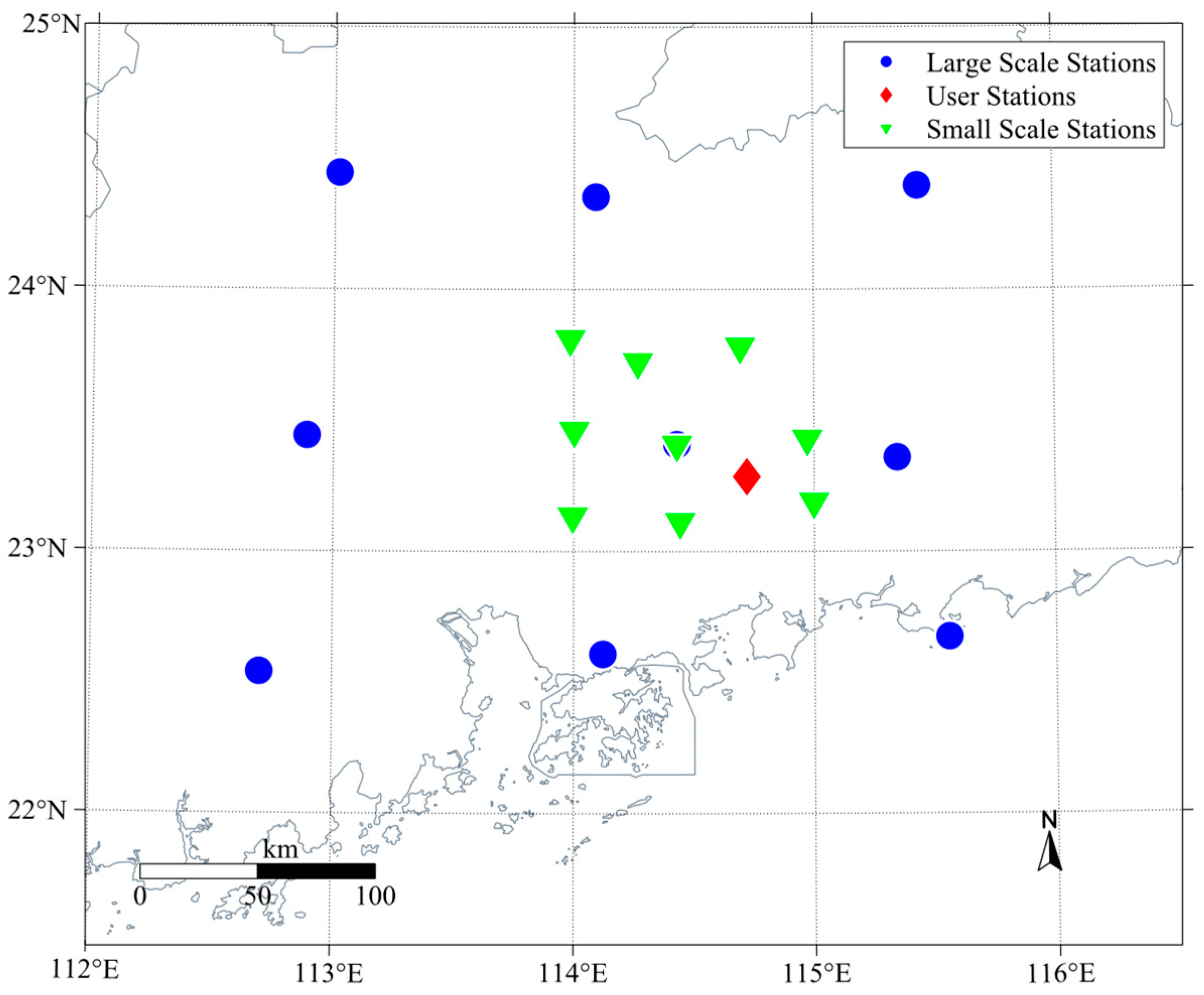
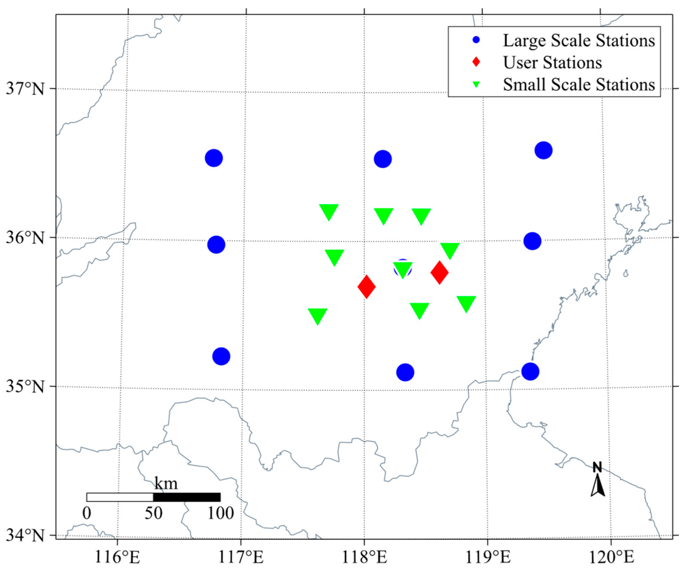
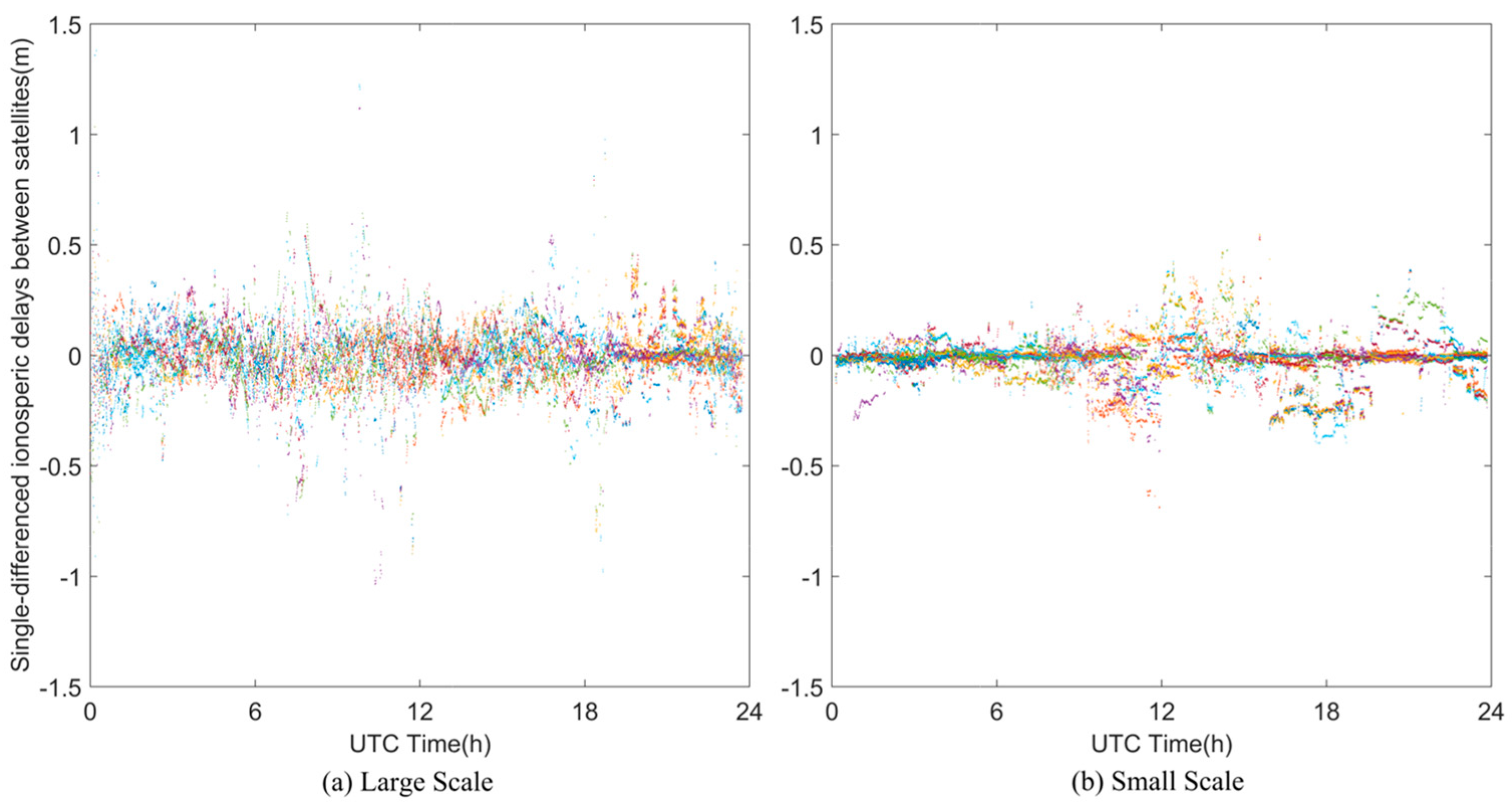
• A systematic investigation of the impact of ionospheric network grid scales (large versus small) on PPP-RTK integrity performance, conducted across diverse latitudinal regions (low-latitude—Guangdong; mid-latitude—Shandong), providing a comprehensive understanding of how modeling scale and ionospheric dynamics jointly affect PL computations;
• The development and application of a statistical modeling approach for PPP-RTK-derived ionospheric residuals, leading to the derivation of robust ionospheric integrity parameters that capture hourly spatiotemporal variability;
• The demonstration, through extensive experimental validation using real GNSS data, that incorporating these refined ionospheric integrity parameters into an ARAIM MHSS framework significantly improves PL accuracy, enhances system availability, and substantially reduces misleading and hazardous outcomes;
• The provision of a validated methodology that offers theoretical support and technical guarantees for achieving higher precision and integrity in GNSS positioning, particularly in regions susceptible to complex ionospheric activity.

The remainder of this paper is structured as follows. Section 2 details the proposed methodology, including the ionospheric error modeling and the integrity monitoring framework. Section 3 presents the experimental setup and discusses the key results obtained from different regional analyses. Finally, Section 4 offers a discussion of the findings and their implications, followed by the main conclusions of this study in Section 5.

2. Materials and Methods

In this section, we focus on the undifferenced and uncombined PPP-RTK technique and the methodology for computing integrity protection levels. To begin, we present a comprehensive flowchart that illustrates the step-by-step process for achieving protection level calculations within high-precision positioning systems. This includes an in-depth explanation of the ambiguity-resolved slant ionospheric observations and the integration of the proposed integrity algorithm.

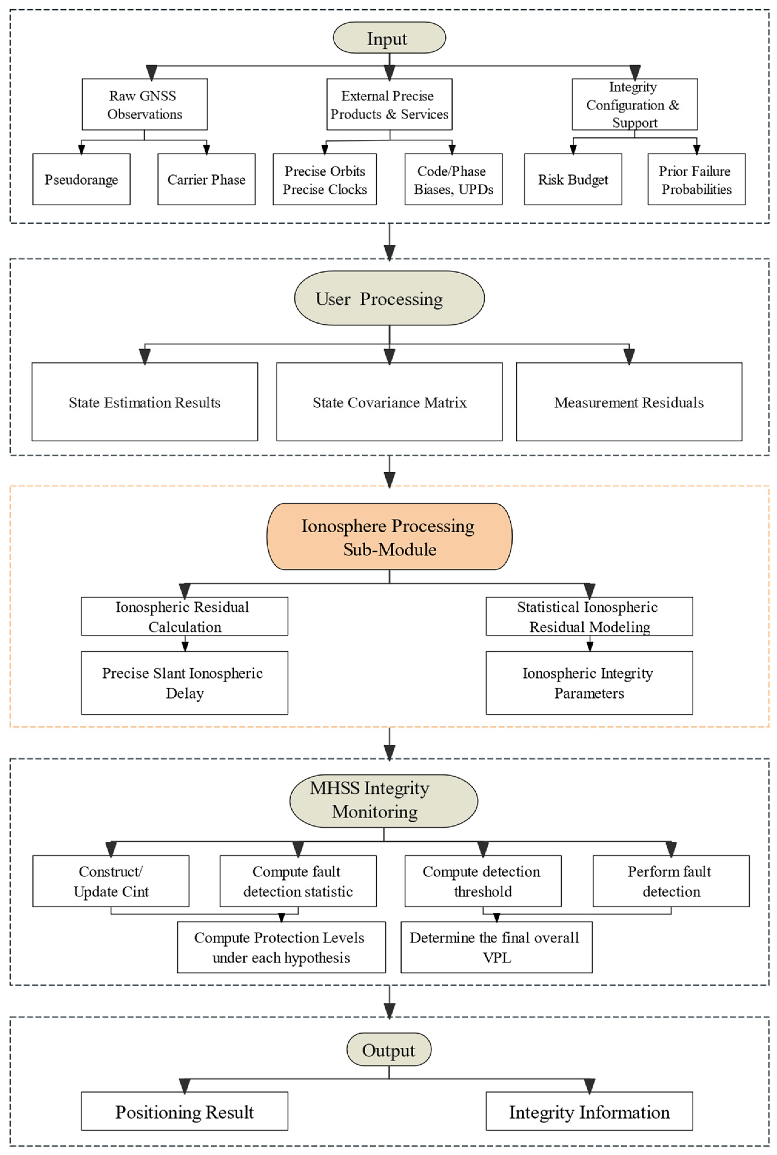
2.1. Experimental Workflow

The overall methodological framework employed in this study is visually summarized in Figure 1. This flowchart outlines the sequential processing stages, beginning with data acquisition and culminating in the provision of precise positioning results augmented with robust integrity information.

The process initiates with the ingestion of essential input data. These inputs are primarily fed into the User Processing stage. Here, an undifferenced and uncombined PPP-RTK engine is utilized to derive core products: the State Estimation Results (including user position, receiver clock offset, tropospheric delay, and resolved ambiguities), the associated State Covariance Matrix, and the Measurement Residuals. A critical output from this stage, feeding into the specialized ionospheric handling, is the Precise Slant Ionospheric Delay.

A key innovative component of this framework is the dedicated Ionosphere Processing Sub-Module, highlighted in the flowchart. This sub-module first performs Ionospheric Residual Calculation using the precise slant ionospheric delays obtained from the User Processing stage. Subsequently, Statistical Ionospheric Residual Modeling is applied to these residuals—involving techniques such as hourly characterization and robust overbounding to derive crucial Ionospheric Integrity Parameters, namely the standard deviation and an extreme error bound for the ionospheric threat.

These statistically derived Ionospheric Integrity Parameters are then critical inputs to the ARAIM Multiple Hypothesis Solution Separation (MHSS) Integrity Monitoring module. This module also utilizes the State Covariance Matrix, Measurement Residuals from the User Processing stage, and the initial Integrity Configuration and Support data. Within this integrity monitoring process, the error covariance matrix is first constructed or updated, crucially incorporating the derived ionospheric standard deviation. Subsequently, fault detection statistics are computed and compared against their corresponding, carefully determined thresholds to identify potential satellite malfunctions. Following the fault detection stage, PLs are calculated under various fault hypotheses, a step where the derived ionospheric extreme error bound serves as a realistic and data-driven ionospheric bias term. From these evaluations, the final overall vertical protection level (VPL) is determined. Furthermore, this module can optionally proceed to assess the Probability of Hazardously Misleading Information (P(HMI)), considering worst-case fault scenarios and the refined ionospheric error characterization.

Finally, the overall process culminates in the Output stage, delivering the user’s Positioning Result along with comprehensive Integrity Information, typically the VPL and, if computed, the P(HMI). The subsequent sections of this paper will elaborate on the theoretical underpinnings and mathematical formulations of each key component within this integrated framework.

2.2. PPP-RTK ARAIM Algorithm Based on MHSS

The core integrity monitoring scheme adopted for PL computation is the ARAIM algorithm, specifically leveraging the MHSS technique [24]. This approach evaluates integrity by extending traditional subset-solution methods. It is designed to process pseudo-range measurements from multiple satellite constellations and can account for various satellite failure modes, including both independent and correlated failures. A key function of this ARAIM algorithm is the computation of the VPL, achieved through an optimal allocation of continuity and integrity risk budgets to ensure navigation performance meets requirements for the specific phase of operation.

2.2.1. Fundamental Observation Model and State Estimation

The foundation of satellite navigation and the ARAIM process lies in the linearized observation model of the navigation system. At each epoch, this model is expressed as

$$y=G{x}^2+{\epsilon }^2$$

(1)

where

y is the vector of observed-minus-computed pseudo-ranges.

G is the observation geometry matrix.

x is the user state vector (position deviations and receiver clock offset).

ε is the measurement error vector, assumed to follow a zero-mean Gaussian distribution.

The user state vector x is estimated using the weighted least squares (WLS) method. Under the fault-free assumption (hypothesis H₀), the state estimate is given by

$$\widehat{{\mathit{x}}_0}={({\mathit{G}}^T{\mathit{W}}_{URA}\mathit{G})}^{-1}{\mathit{G}}^T{\mathit{W}}_{URA}\mathit{y}={\mathit{S}}_0\mathit{y}$$

(2)

where $S_0$ is the WLS projection matrix under the fault-free assumption and $W_{URA}=C_{int}^{-1}$ is the weighting matrix. $C_{int}$ is the covariance matrix of pseudo-range measurements under the integrity nominal error model. The diagonal elements of $C_{int}$ (assuming uncorrelated measurement errors between satellites for this representation), or more generally, the variance ${\sigma }_k^2$ for the pseudo-range measurement of each satellite k, is a composite of several error sources:

$${\sigma }_k^2={\mathit{\sigma }}_{URA,k}^2+{\mathit{\sigma }}_{tropo,k}^2+{\mathit{\sigma }}_{user,k}^2+{\mathit{\sigma }}_{iono,k}^2$$

(3)

In this composite error model,

${\mathit{\sigma }}_{URA,k}^2$ accounts for errors originating from the ground segment, including satellite clock and ephemeris inaccuracies;

${\mathit{\sigma }}_{tropo,k}^2$ represents the variance due to tropospheric signal delay;

${\mathit{\sigma }}_{user,k}^2$ encompasses user-equipment-specific errors such as receiver noise and multipath effects. These non-ionospheric components are typically characterized using established standard models and parameters.

However, the characterization of the ionospheric error component, ${\mathit{\sigma }}_{iono,k}^2$, presents a distinct challenge. Unfortunately, no universally accepted, clear formula has been proposed for precisely calculating the ionospheric error for integrity purposes. Some authors have proposed treating the ionospheric error as a constant value for calculation [25,26,27]. A key point contradictory to this simplification, however, is that the ionospheric error exhibits obvious and significant spatiotemporal characteristics. This inherent variability is the primary reason why this study investigates the hourly error distribution of the ionosphere, as detailed in subsequent sections. Concurrently, the main exploration of this research is reflected in the novel way that these characterized ionospheric errors participate in the integrity calculation framework. The primary innovation of this work, detailed in Section 2.3, is a methodology for deriving robust ${\mathit{\sigma }}_{iono,k}^2$ values based on statistical analysis of PPP-RTK derived ionospheric residuals, which are then incorporated into this error budget for comprehensive integrity calculations.

2.2.2. Fault Detection and Protection Level Computation

Within the ARAIM MHSS framework, multiple potential fault scenarios are evaluated. Under a specific fault hypothesis $H_k$, which assumes the measurement from the k-th satellite is erroneous, a dedicated state vector estimate $\widehat{{\mathit{x}}_k}$ is calculated. This calculation involves appropriately adjusting the standard WLS estimation procedure to eliminate or de-weight the contribution of the potentially faulty k-th measurement, resulting in

$$\widehat{{\mathit{x}}_k}=S_{k}y$$

(4)

where $S_k$is the projection matrix pertinent to the $H_k$ scenario.

To test the validity of hypothesis $H_k$, a dedicated statistic $d_k$ is formulated. This statistic measures the solution separation induced by assuming the k-th fault, commonly achieved by comparing the $H_k$ solution to the nominal fault-free solution $\widehat{{\mathit{x}}_0}$:

$$d_k=\left|{\widehat{\mathit{x}}}_k-{\widehat{\mathit{x}}}_0\left|=\right|{\mathit{S}}_k-{\mathit{S}}_0\right|y$$

(5)

A decision regarding fault detection is made by evaluating d_k relative to a threshold $D_k$:

$$D_k=K_{ffd,k}\times {\sigma }_{dV,k}+{\displaystyle \sum }_{i=1}^n\mid \Delta {\mathit{S}}_k\left(3,i\right)\mid \times b_{norm}$$

(6)

The value of $D_k$ is determined by the acceptable false alarm rate, reflecting the test statistic’s expected noise (${\sigma }_{dV,k}$) and systematic biases ($b_{norm}$), appropriately scaled by factors such as $K_{ffd,k}$. If $d_k$ > $D_k$, a fault is declared.

The overall VPL is then the maximum of the VPL for the fault-free case and for each considered fault hypothesis:

$$V_{\mathrm{PL}}=max\left\{V_{\mathrm{PL}\left(0\right)},V_{\mathrm{PL}(k)}\right\},k=0,\dots ,n$$

(7)

For the scenario where no satellite faults are present, the corresponding protection level, $V_{\mathrm{PL}\left(0\right)}$, is formulated as below. Conversely, when a fault is assumed to be associated with the k-th satellite, the protection level, $V_{\mathrm{PL}(k)}$, is determined by taking into account the detection threshold $D_k$, specific to that fault mode:

$$V_{\mathrm{PL}\left(0\right)}=K_{md,0}\times {\sigma }_{V,0}+{\displaystyle \sum }_{i=1}^n\mid {\mathit{S}}_0\left(3,i\right)\mid \times b_{\max }$$

(8)

$$V_{\mathrm{PL}\left(k\right)}=D_k+K_{md,k}\times {\sigma }_{V,k}+{\displaystyle \sum }_{i=1}^n\mid {\mathit{S}}_k\left(3,i\right)\mid \times b_{\max }$$

(9)

In these protection level equations, the coefficients $K_{md,0}$ and $K_{md,k}$ are crucial multipliers, derived from the allocated integrity risk for missed detections. $K_{md,0}$ scales the error statistics for the nominal, fault-free operational state, ensuring the integrity requirement is met. Similarly, $K_{md,k}$ applies to the scenario where the k-th satellite is the presumed source of failure, ensuring the integrity budget is maintained under this specific fault condition. The terms ${\sigma }_{V,0}$ and ${\sigma }_{V,k}$ represent the standard deviation of the vertical positioning error under the respective hypotheses; $S_0\left(3,i\right)$ and $S_k\left(3,i\right)$ denote the sensitivity of the vertical position solution to the i-th measurement for the fault-free and k-th fault hypothesis, respectively. A key aspect of this study is the incorporation of the statistically derived ionospheric error standard deviation, ${\sigma }_{iono}$, into the calculation of these vertical error standard deviations. Specifically, σiono2 contributes as a component to the total variance budget used to determine ${\sigma }_{V,0}$ and ${\sigma }_{V,k}$, thereby reflecting the refined ionospheric uncertainty. $b_{\max }$ is a term accounting for the maximum potential bias contributions.

2.2.3. Integrity Risk Evaluation

Beyond the calculation of protection levels, a direct assessment of the integrity risk is crucial. The framework for this integrity risk evaluation, including the definition of Hazardously Misleading Information (HMI) and the subsequent methodological steps, is adapted from the approach detailed in [28].

Integrity risk is quantitatively defined as the probability of HMI, P(HMI). HMI occurs if the actual positioning error, denoted ${\epsilon }_k$, in a dimension of interest exceeds its corresponding Alert Limit (AL), while this hazardous condition is not detected by the integrity monitoring system. This can be expressed as

$$P(HM{I}_k)=P(\left|{\epsilon }_k\right|>AL)\cap fault not detected$$

(10)

The evaluation of $P(HM{I}_k)$ requires considering various potential fault modes ($hi$). Each fault mode hi, representing a specific fault or combination of faults, has an associated prior probability of occurrence, $P\left(hi\right)$. The total integrity risk is then computed by summing the conditional probability of HMI given each fault mode, $P(HM{I}_k|hi)$, over all relevant fault modes, weighted by their respective probabilities:

$$P(HM{I}_k)\approx {{\displaystyle \sum }}_{i}P(HM{I}_k|hi)P\left(hi\right)+P_{unevaluated}$$

(11)

In this summation, $P_{unevaluated}$ accounts for the residual risk from fault modes that are not explicitly evaluated, typically those with very low prior probabilities of occurrence.

To determine $P(HM{I}_k|hi)$ for each considered fault mode, it is necessary to characterize the distributions of the position error ${\epsilon }_k$ and the fault detection statistic (such as dk discussed earlier, or an equivalent detector as outlined in the reference methodology) under that specific fault mode $hi$. A critical aspect of this process, as detailed in the adopted framework [28], is the identification of the “worst-case” fault scenario for each mode hi. This involves finding the fault magnitude and characteristics that maximize $P(HM{I}_k|hi)$. Such an analysis typically involves examining the impact of potential faults on the expectation (mean) of the position error and on the non-centrality parameter of the fault detector’s statistical distribution. Furthermore, to manage computational complexity while ensuring a comprehensive assessment, the analysis of fault modes may be confined to a specific time window, with conservative assumptions made for the influence of faults occurring prior to this window.

2.3. Statistical Ionospheric Error Modeling Using Undifferenced and Uncombined PPP-RTK for Integrity Parameter Derivation

To obtain the high-fidelity ionospheric information necessary for robust integrity parameter derivation, this study employs an undifferenced and uncombined PPP-RTK approach. This method processes raw pseudo-range and carrier phase observations, thereby avoiding the information loss and potential noise amplification often associated with traditional ionosphere-free combinations. The selection is further motivated by its adaptability and its inherent advantages for integrity-focused applications. For instance, as noted by Zhang et al. [29], the undifferenced and uncombined PPP-RTK framework offers greater flexibility in accommodating dynamic constraints on parameters within the positioning algorithm. From the perspective of system integrity, the preservation of a richer set of observation data, combined with rigorous product evaluation, facilitates more accurate prediction and estimation of localization errors. This comprehensive data handling is instrumental in supporting a lower probability of false alarms.

The functional model for pseudo-range (P) and carrier phase (L) observations is

$$\left\{\begin{array}{l}{P}_{r,i}^s={\rho }_r^s+cd{t}_r-cd{t}^s+T_r^s+I_{r,i}^s+b_{r,i}-b_i^s+{\epsilon }_{i,P}^s\\ L_{r,i}^s={\rho }_r^s+cd{t}_r-cd{t}^s+T_r^s-I_{r,i}^s+{\lambda }_i^s\left(N_{r,i}^s+B_{r,i}-B_i^s\right)+{\epsilon }_{i,\phi }^s\end{array}\right.$$

(12)

In these observation equations, the terms have the following significance: $P_{r,i}^s$ and $L_{r,i}^s$ represent the pseudo-range and carrier-phase measurements, respectively, both expressed in units of meters. The geometric distance linking satellite s and receiver r is denoted by ${\rho }_r^s$. Signal propagation delays are accounted for by $T_r^s$ for the tropospheric path delay and $I_{r,i}^s$ for the frequency-dependent ionospheric path delay. Timing aspects involve c, the vacuum speed of light, and the clock offsets of the receiver ($d{t}_r$) and satellite ($d{t}^s$), given in equivalent distance units. Specific to the carrier phase measurement are ${\lambda }_i^s$, the wavelength of the carrier signal, and $N_{r,i}^s$, the integer ambiguity representing the unknown number of full cycles. Instrumental biases originating from hardware include code biases ($b_{r,i}$ for receiver, $b_i^s$ for satellite) and phase biases ($B_{r,i}$ for receiver, $B_i^s$ for satellite). Finally, the terms ${\epsilon }_{i,P}^s$ and ${\epsilon }_{i,\phi }^s$ capture the unmodeled errors, such as measurement noise and multipath, inherent in the respective pseudo-range and carrier-phase observations.

Using precise satellite products (orbits, clocks, Uncalibrated Phase Delays (UPDs)), slant ionospheric delays (${\tilde{I}}_{r,1}^s$) are derived from carrier phase observations after ambiguity resolution. These derived delays are biased measures of the true ionospheric delay, containing hardware biases.

$$\begin{array}{l}{\tilde{I}}_{r,1}^s=L_{r,1}^s-\left({\rho }_r^s+cd{t}_r-cd{t}^s+T_{r,w}^s+T_{r,d}^s+{\lambda }_1^s{N}_{r,1}^s-{\lambda }_1^s{d}_1^s\right) \\ =I_{r,1}^s+{\displaystyle \frac{c\cdot f_2^2}{f_2^2-f_1^2}}\left(DC{B}_{r,12}-DC{B}_{12}^s\right)+{\lambda }_1^s{d}_{r,1}+{\epsilon }_{1,\phi }^s \\ =I_{r,1}^s+{ \mathrm{bias} }_r-{ \mathrm{bias} }^s+{\epsilon }_1^s\end{array}$$

(13)

The derived slant ionospheric delay, ${\tilde{I}}_{r,1}^s$, on the L1 frequency is obtained after accounting for tropospheric effects. The hydrostatic tropospheric delay $T_{r,d}^s$ is computed using a standard empirical mode. The tropospheric wet delay $T_{r,w}^s$ is estimated as a Zenith Wet Delay parameter within the undifferenced and uncombined PPP-RTK state vector, subsequently projected to the slant path. Subtracting these tropospheric components isolates ${\tilde{I}}_{r,1}^s$, which then contains the desired ionospheric delay, along with residual tropospheric errors and system biases, for further statistical processing.

The core of our ionospheric integrity approach then lies in the statistical characterization of hourly ionospheric residuals derived from such undifferenced and uncombined PPP-RTK processing. This process, informed by the observed characteristics of these residuals, is performed as follows:

• Ionospheric delay residuals are grouped on an hourly basis to capture their temporal characteristics. For each hourly dataset, a Laplace distribution is fitted to the residuals. The choice of the Laplace distribution is motivated by its suitability for modeling data with a sharper peak and heavier tails compared to a Gaussian distribution, characteristics often observed in ionospheric error residuals, particularly during active conditions. This fitting provides a robust estimation of the distribution’s scale parameter, which is directly related to the standard deviation (STD) for that hour and is less sensitive to outliers than a direct sample STD.
• While the Laplace distribution effectively models the bulk of the residuals, for integrity applications, a conservative overbounding model is required to account for uncharacteristically large errors. For each hour, a zero-mean Gaussian distribution is determined such that its cumulative distribution function conservatively overbounds the cumulative distribution function of the fitted Laplace distribution for the tail regions relevant to integrity. The standard deviation of this overbounding Gaussian distribution, denoted ${\sigma }_{\mathrm{iono},\mathrm{Gauss}}$, is then taken as the equivalent STD, ${\sigma }_{\mathrm{iono}}$, for that hour. This ensures that the probability of the true error exceeding a certain bound, as predicted by the Gaussian model, is greater than or equal to the probability predicted by the Laplace or empirical distribution, providing a conservative estimate of ionospheric uncertainty.
• Using the parameters of the conservative Gaussian overbounding model determined in the previous step, the extreme error bound, $b_{iono}$, is computed. This bound corresponds to the quantile of the zero-mean Gaussian distribution associated with the target probability of hazardous misleading information allocated to the ionospheric threat for a single satellite, $P_{HMI,iono}$. For high-integrity applications, this probability is typically very small. For instance, if the integrity risk allocation for ionospheric hazardous events per satellite is $P_{HMI,iono}=Q\times {10}^{-7}$, where Q is a factor, often related to the number of satellites or specific operational requirements, sometimes simplified such that the tail probability directly relates to a multiple of 10⁻⁷, then $b_{iono}$ is calculated as

  $$b_{iono}=K_{iono}\times {\sigma }_{iono}$$

  where $K_{iono}$ is the multiplier (quantile) obtained from the inverse standard normal distribution corresponding to the one-sided tail probability $P_{HMI,iono}$/2. For example, a tail probability on the order of 5 × 10⁻⁸ would correspond to a $K_{iono}$ value of approximately 5.33 to 5.6, depending on the exact probability and whether one or two-sided bounds are considered for a particular PL equation component. This $b_{iono}$ then serves as the ionospheric bias term in the PL calculations.

These statistically derived ionospheric parameters—the hourly STDs and the extreme error bounds—are critical inputs. The STDs are used to populate the ionospheric component of the $C_{int}$ matrix, directly influencing $W_{URA}$ and thus the precision of the state estimate and the derived VPL. The extreme error bound serves as a data-driven ionospheric bias parameter that can replace or augment generic bias terms in the VPL equations and in the assessment of $P(HM{I}_k|hi)$ under worst-case ionospheric conditions. This provides a more realistic and dynamic representation of ionospheric threats within the overall integrity framework.

3. Results

Static tests were conducted using multi-constellation observation data from GPS, Galileo, and BeiDou, sampled at 30 s intervals over a period of seven days. Accurate satellite orbits and clock corrections were sourced from GFZ (German Research Centre for Geosciences) Global Bias Model (GBM), while code bias corrections were obtained from Chinese Academy of Sciences (CAS). To evaluate and compare ionospheric activity between mid-latitude and low-latitude regions, data from 37 stations were utilized, with 18 stations in Guangdong Province (low-latitude, 23.13° N, 113.28° E) and 19 stations located in Shandong Province (mid-latitude, 36.65° N, 117.11° E). In each province, the stations were further organized into two network configurations: a large-scale network with station spacings of approximately 150 km and a small-scale network with spacings of about 50 km. This dual-network approach allowed for comprehensive modeling of ionospheric behavior at different spatial scales.These stations were equipped with dual-frequency GNSS receivers and operated under stable environmental conditions, ensuring high-quality data. Additionally, all stations participated in the estimation of UPD, which provided valuable insights into ionospheric residuals. The data collection process was continuous, with a consistent sampling frequency, enabling detailed temporal and spatial analysis of ionospheric activity.

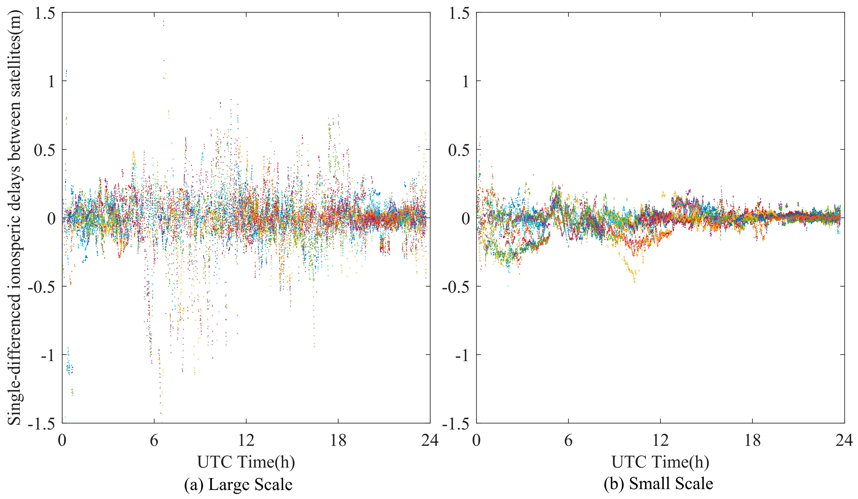
3.1. Ionospheric Modeling in Mid and Low Latitudes

To evaluate the impact of ionospheric residuals at different modeling scales on the computation of protection levels in GNSS integrity monitoring, a total of 18 monitoring stations were selected from the Guangdong region. These stations were divided into two groups to represent distinct spatial scales of ionospheric modeling as introduced above.

This dual-network configuration provides a comprehensive framework for examining how the spatial density of reference stations influences the magnitude of ionospheric residuals and, subsequently, the derived protection levels. By employing consistent observational data and computational methodologies across both networks, the experimental design ensures a controlled and systematic comparison between the two scales. This analysis is particularly relevant in understanding the trade-offs between modeling accuracy and resource allocation in ionospheric correction systems, thereby addressing a critical challenge in achieving robust GNSS integrity in ionospheric-disturbed environments.

Figure 2 depicts the distribution of stations in Guangdong Province, with blue circles denoting reference stations of the large network, green triangles representing reference stations of the small network, and red diamonds representing user stations. The analysis began by constructing a grid data file based on reference stations, followed by evaluating their impact on the user stations. The dataset utilized corresponds to observations collected on 14 October 2022 (Day of Year (DOY): 277), a day characterized by relatively calm geomagnetic conditions (Kp = 2.92, Dst = −19.6 nT).

In the Guangdong region, a comparative analysis of ionospheric residuals was conducted using grids of different spatial scales. The results, contrasting large-scale and small-scale grid networks, reveal significant disparities in ionospheric residual behavior. Specifically, the large-scale grid network exhibits substantial and pronounced fluctuations in ionospheric residuals, whereas the small-scale grid network demonstrates considerably smoother and more stable residual patterns, as shown in Figure 3. These findings underscore the influence of grid scale on ionospheric modeling accuracy, with larger grids being less capable of capturing localized ionospheric variations. Recent studies have demonstrated that the use of small-scale reference networks significantly improves the accuracy of ionospheric delay modeling, enhancing the convergence and precision of PPP-RTK positioning [30].

To generalize the findings across different latitudinal conditions, the analysis was extended to a relatively stable mid-latitude environment. Figure 4 shows the distribution of 19 stations located in Shandong Province. The data utilized for this analysis were collected on 28 September 2022 (DOY: 271), a day characterized by mild geomagnetic activity with indices of Kp = 0.83 and Dst = −13.8 nT, ensuring consistency with previous observations.

To further investigate the impact of ionospheric residuals on GNSS protection level computations, an additional network was established in the Shandong region, employing a similar dual-scale design to that of Guangdong. The Shandong network also comprises 19 monitoring stations, divided into a large-scale network and a small-scale network. This parallel setup facilitates a consistent comparison of ionospheric modeling performance across different spatial scales. However, compared to Guangdong, the ionospheric conditions in Shandong are notably more stable, reflecting the region’s predominantly mid-latitude characteristics with less pronounced ionospheric fluctuations.

By incorporating both regions into the analysis, this study provides a comprehensive evaluation of how ionospheric variability and modeling scale jointly influence protection level (PL) computations. The findings demonstrate that ionospheric residuals are shaped not only by grid scale but also by latitude-dependent ionospheric dynamics. This variability, if not properly modeled, leads to discrepancies between simplified constant-error assumptions and the true error behavior observed in real environments, particularly under low-latitude, high-variability conditions. Similar findings have been reported by Zhao et al., who demonstrated that precise ionospheric corrections derived from multi-scale reference networks can significantly enhance GNSS positioning performance, even under low solar activity conditions [31]. Moreover, Liu et al. proposed advanced interpolation methods to further refine the generation of regional ionospheric corrections, emphasizing the importance of high-precision modeling under sparse network conditions [32].

In the Shandong region, a similar analysis was conducted as in Guangdong, examining the impact of ionospheric residuals at different spatial scales. However, due to the geographical location of Shandong in a mid-latitude zone, the ionospheric behavior is relatively more stable compared to the low-latitude Guangdong region, as shown in Figure 5. As a result, the ionospheric influence on positioning accuracy in Shandong is less pronounced. Despite this, the analysis still reveals significant variations in ionospheric residuals across different grid scales, mirroring the findings observed in Guangdong. Similar findings have been reported by Zhao et al., who demonstrated that the scale of the reference network significantly affects the modeling of ionospheric residuals and the convergence performance of PPP-RTK solutions [33]. Additionally, grid-based ionospheric weighting strategies have been shown to further reduce PPP-RTK convergence times under diverse network configurations and varying ionospheric activity levels, highlighting the importance of adopting adaptive modeling approaches in integrity-critical applications [34]. This provides an additional layer of comparison, specifically highlighting the differences in ionospheric characteristics between mid-latitude and low-latitude regions.

This comparison underscores the notion that ionospheric residuals are not only influenced by the spatial grid scale but also by the latitude of the region. The dynamic nature of the ionosphere varies significantly between latitudes, and consequently, the ionospheric residuals and their effects on positioning accuracy differ. In this context, if ionospheric residuals are modeled as constant values and incorporated into PL computations, even in relatively stable mid-latitude regions like Shandong, the result would still lead to errors that deviate from the true positioning errors. The simplified approach of treating ionospheric errors as constants fails to capture the complex spatiotemporal characteristics of the ionosphere, which is crucial for accurate integrity assessment.

The findings from both Guangdong and Shandong regions underscore the significance of accounting for the spatial and temporal variability of ionospheric residuals, particularly when modeling them across different grid scales. This variability, along with the ionosphere’s complex spatiotemporal characteristics, is crucial for generating more accurate and reliable protection levels. Our research highlights the necessity of incorporating detailed ionospheric residuals—representing the true dynamic behavior of the ionosphere at varying scales and latitudes—into protection level calculations to ensure more dependable GNSS integrity assessments. These insights directly inform the methodology and the results, providing a clear foundation for subsequent discussions on the enhancement of GNSS performance.

3.2. User-Side Protection Level Calculation

Building on the residual analysis, user-side PL calculations were conducted by integrating ionospheric integrity parameters derived from the observed residual distributions. STD was determined by enveloping 98% of the data points within a Gaussian distribution, forming the basis for dynamic PL computation.

The integrity parameters presented in

Table 1. Key parameters for GNSS integrity assessment.

Category	Parameters	Value
Prior Probabilities	$P_{\mathrm{sat},j}$ (Satellite j fault)	$1\times {10}^{-5}$
	$P_{\mathrm{const},j}$ (Constellation j fault)	$1\times {10}^{-8}$
	$P_{\mathrm{iono},\mathrm{i}}$ (Ionospheric anomaly i)	$1\times {10}^{-5}$
	$P_{\mathrm{trop}}$ (Tropospheric anomaly)	$1\times {10}^{-6}$
URE Standard Deviations	${\sigma }_{URE, pseudorange}$	$1 \mathrm{m}$
	${\sigma }_{URE, phase}$	$1/100 \mathrm{cycles}$
	${\sigma }_{URE, iono}$	$0.06 \mathrm{m}$
	${\sigma }_{URE,trop}$	$0.03 \mathrm{m}$
Other Integrity Parameters	$b_{nominal}$ (Nominal bias bound)	$3/4 {\sigma }_{URE}$
	$P_{threshold}$ (Detection threshold allocation)	$6\times {10}^{-8}$

, particularly the prior probabilities of satellite, constellation, and atmospheric anomalies, as well as nominal bias bounds and User Range Error (URE) standard deviations, are largely based on or adapted from the baseline ARAIM user algorithm specifications and typical values discussed in foundational studies such as Blanch et al. [22]. These parameters are commonly adopted in ARAIM research to represent nominal system performance. The URE standard deviation for the carrier phase is set to 0.01 cycles. This value aligns with the typical standard deviation for undifferenced carrier phase observation noise used in precise positioning applications, such as that adopted by Zhang and Wang [23]. For its application in the protection level equations, where errors are typically characterized in meters, this cycle-based standard deviation is converted to meters by multiplying with the respective carrier wavelength during the formation of the observation covariance matrix or in subsequent error propagation steps.

Previous studies have emphasized the importance of defining ionospheric integrity parameters for the precise calculation of PLs. These parameters allow for the dynamic adjustment of protection thresholds, ensuring that navigation systems can meet positioning requirements under varying environmental conditions while enhancing the overall robustness and reliability of the system. Comparative analysis of positioning errors, achieved by integrating ionospheric integrity parameters with PL calculations, demonstrates that such integration can significantly improve system stability and accuracy under anomalous ionospheric conditions. Specifically, in mid-latitude regions, the introduction of ionospheric integrity parameters results in tighter PL bounds, more effectively reflecting actual risk levels. In low-latitude regions, where ionospheric activity is more complex, this integration enables the timely identification and mitigation of potential hazardous information, thereby reducing false alarm rates and improving positioning reliability.

The next section will provide a detailed discussion of the PL calculation results incorporating ionospheric information, with a focus on the tightness of PL bounds in mid-latitude regions and the effective mitigation mechanism for hazardous information in low-latitude regions.

Figure 6 presents a comparative analysis of horizontal positioning error (HPE), vertical positioning error (VPE), and their corresponding PLs over a 4 h observation period in the mid-latitude region (corresponding to the large ionospheric modeling network in Figure 4) on 28 September 2022 (DOY: 271). The upper panel illustrates the results for the horizontal domain, displaying HPE (blue line) and the associated PLs (shaded area), while the lower panel shows the results for the vertical domain, presenting VPE (blue line) and its corresponding PLs (shaded area).

During the observation period, both horizontal and vertical positioning errors exhibit a notable convergence trend within the first hour, followed by a period of stabilization. The PL intervals are represented by two types of shading—dark shading corresponds to the PL derived from the ionosphere-enhanced method, while light shading represents the conventional PL computed without incorporating ionospheric variability. The results indicate that, compared to the traditional approach, integrating ionospheric information leads to significantly narrower PL bounds in the mid-latitude region. This enhancement contributes to a reduction in overbounding and a lower false alarm rate. Given the relatively stable ionospheric activity in mid-latitude regions, using fixed error assumptions tends to be overly conservative, which increases the likelihood of unnecessary alerts. In contrast, the proposed method, which accounts for ionospheric variability, alleviates this limitation by more accurately characterizing actual positioning uncertainties.

In addition, the horizontal positioning errors are generally smaller than their vertical counterparts, and the corresponding PLs are more constrained, reflecting the typical disparity in directional uncertainty within GNSS positioning. Despite this inherent vertical sensitivity, the enhanced ionospheric correction model maintains the vertical PLs within acceptable bounds. The comparative results presented in Figure 6 substantiate the effectiveness of the ionospheric-enhanced approach in improving both horizontal and vertical protection level computations under mid-latitude conditions. The following section presents the outcomes of protection level calculations that incorporate ionospheric information, specifically within the low-latitude region. This part focuses on the analysis of the influence of ionospheric information on the calculation of PLs during the 6 h reconvergence process. This analysis aims not only to assess the role of ionospheric information in positioning accuracy, but also to highlight its critical influence in the convergence phase. Since the ionospheric error has a significant impact on the convergence process of the solution, adding ionospheric information in the convergence stage can better optimize the protection level calculation and improve the performance of the system in the unstable state.

Extending the analysis to the low-latitude region, Figure 7 shows the temporal evolution of positioning error and the corresponding protection levels, PL1 and PL2, in the east component over a 6 h observation period on 14 October 2022 (DOY: 277). The experiment adopts an hourly reinitialization scheme to evaluate system behavior during repeated convergence under dynamic ionospheric conditions, based on the large-scale modeling network shown in Figure 2.

At the beginning of each reinitialization cycle, the PE—represented by red markers—exhibits significant fluctuations, followed by gradual stabilization as the solution converges. PL1, shown in green, is computed without accounting for ionospheric variability and often tracks the PE too closely. This limited error margin increases the likelihood of missed detections, especially during the early convergence phase when positioning errors are large and ionospheric disturbances are more prominent.

In contrast, PL2 (blue) incorporates ionospheric error modeling and maintains a more adaptive protection envelope. It provides sufficient separation from the PE, resulting in a notable reduction in missed detections without introducing excessive overbounding. As the system transitions to a steady state, PL2 continues to preserve a safe margin, thereby offering improved integrity performance in complex ionospheric environments.

Table 2. Performance comparison of traditional and ionosphere-enhanced protection levels (PL1 vs. PL2) in low-latitude region.

	PL 1	PL 2
Normal	60.50%	94.70%
Misleading	35.20%	4.10%
Hazardous	2.80%	0.50%
Unavailable	1.50%	0.70%

provides a quantitative comparison of the performance of PL1 and PL2 in the low-latitude region. The results show that PL2 significantly improves the system’s reliability, with the Normal condition percentage increasing from 60.5% for PL1 to 94.7% for PL2. Additionally, PL2 reduces the Misleading cases from 35.2% to 4.1%, highlighting its ability to more accurately bound the PE. The Hazardous cases are also reduced from 2.8% to 0.5%, indicating fewer unnecessary alerts, while the Unavailable cases decrease slightly from 1.5% to 0.7%, reflecting improved system reliability. It can be directly attributed to the incorporation of the refined ionospheric integrity parameters derived from the statistical modeling approach presented in Section 2.3.

In the low-latitude region, where ionospheric activity is highly dynamic, the green-marked regions corresponding to PL1 exhibit a critical issue of missed detections due to the protection level being overly close to the PE. Conversely, the blue-marked regions of PL2 show a notable reduction in missed detections, underscoring the advantage of the ionosphere-enhanced model in mitigating this limitation. Particularly during the steady-state phase of PE, PL2 maintains safety while significantly reducing overbounding phenomena, thereby enhancing the reliability of GNSS integrity monitoring.

These findings, supported by both Figure 7 and Table 2, demonstrate the critical importance of incorporating ionospheric information into protection level calculations, particularly in regions with complex ionospheric activity. The ionosphere-enhanced model not only provides more accurate and reliable protection levels but also significantly reduces the risk of missed detections and unnecessary alerts, offering a robust solution for high-integrity GNSS applications.

4. Discussion

The findings of this study inform the design and operation of GNSS integrity monitoring systems, particularly those requiring high reliability. The use of small-scale ionospheric grid models, which reduced residual standard deviations by up to 30% in active low-latitude regions, directly translates into more precise and dependable PLs. Such PLs can improve system availability by reducing the conservatism often associated with cruder error models, without compromising safety. The observed reduction in missed detections is pertinent to safety-of-life applications where unmitigated faults pose risks.

This research highlights a limitation in many conventional integrity algorithms: treating ionospheric errors as static values. This approach does not adequately capture the ionosphere’s dynamic nature, especially during high activity or in regions like the equatorial anomaly. Incorporating a dynamic, spatiotemporally varying ionospheric residual model, as demonstrated in this study, offers a method to address these limitations. By ensuring that protection level calculations are more closely aligned with the actual error distributions experienced by users, integrity assessments better reflect operational conditions. This closer alignment contributes to user confidence and supports GNSS application in sensitive domains, particularly for enhancing integrity in regions with complex ionospheric conditions.

While the findings of this study demonstrate clear improvements, certain limitations should be acknowledged, offering avenues for future refinement. The statistical ionospheric models were derived using datasets spanning specific observation period. The long-term performance and adaptability of these hourly models under a wider range of solar activity levels and during severe geomagnetic storm events warrant further investigation. Although this study focused on regions in China, the direct applicability and potential need for regional tuning of the derived statistical parameters for other geographical areas with different ionospheric climatology also require more extensive validation. Furthermore, while the proposed server-to-user parameter transmission aims to simplify user-end processing, the computational aspects of updating and applying these dynamic ionospheric integrity parameters on resource-constrained user devices, especially at high update rates, could be explored in more detail. The potential influence of unmodeled errors within the PPP-RTK-derived ionospheric residuals on the statistical characterization is another area for ongoing research.

Future work can build upon these findings. Leveraging multi-frequency GNSS signals—including increasingly available triple or even quad-frequency observations—offers a path to more advanced ionospheric error modeling by improving the separation of ionospheric delays from other error sources, such as multipath and observation noise, and from the geometric range. This can facilitate more accurate TEC models and refined integrity parameters for PL calculations beyond dual-frequency capabilities. Furthermore, integrating real-time ionospheric monitoring data from sensor networks could enable dynamic adjustment of error models and PLs in response to current conditions. Such adaptability would enhance system robustness, particularly during space weather events, transitioning from historical statistical models to more proactive threat mitigation. Continued exploration in these areas can further advance the reliability and safety of GNSS integrity applications.

5. Conclusions

This study systematically investigated the critical impact of ionospheric residual modeling on the calculation of PLs for GNSS integrity applications. By comparing ionospheric models at different spatial grid resolutions—large-scale versus small-scale—across two representative regions with distinct ionospheric characteristics, namely Guangdong (low-latitude) and Shandong (mid-latitude), this research has yielded several key findings.

Experimental results clearly revealed the inherent limitations of large-scale grid models in accurately capturing localized and rapid ionospheric variations. These limitations were particularly evident in the low-latitude Guangdong region. In contrast, the application of small-scale grids demonstrated markedly higher effectiveness in representing the complex spatiotemporal dynamics of the ionosphere. As supported by detailed experimental data, the enhanced ionospheric model based on small-scale grids led to substantial improvements in system reliability metrics. This included a notable increase in the percentage of operations under “Normal” conditions, alongside significant reductions in instances of “Misleading Information” and “Hazardous Misleading Information”, and an effective mitigation of missed fault detections. These outcomes collectively underscore the crucial role of higher-resolution modeling in enhancing the precision of positioning performance and the accuracy and reliability of PLs.

Quantitative analysis further substantiates the superiority of refined spatial modeling. For instance, in the challenging low-latitude environment, the implementation of a small-scale grid model not only reduced the standard deviation of ionospheric residuals by approximately 30%, directly contributing to tighter and more consistent PL calculations, but also led to a slight decrease in system “Unavailable” instances. Moreover, this study confirmed that traditional approaches treating ionospheric errors as constant values, especially during active ionospheric periods, result in discrepancies between computed protection bounds and actual positioning error trends.

Therefore, the principal conclusion of this work is that dynamic, high-resolution ionospheric residual modeling, which accurately reflects spatiotemporal variability, is crucial for aligning protection level calculations with real-world error distributions. Such a refined methodology, by reducing missed detection rates, minimizing unnecessary alerts, and enhancing system availability, is paramount for substantially improving the overall reliability and integrity of GNSSs, particularly in regions with complex and volatile ionospheric conditions.

References

1. Working Group C. ARAIM Technical Subgroup Milestone 3 Report of the EU-US Cooperation on Satellite Navigation. Working Group C. 2016. Available online: https://www.gps.gov/policy/cooperation/europe/2016/working-group-c/ (accessed on 13 July 2023).
2. Chang, J.; Qu, Z.; Lian, X.; Wang, Z. Impact of Temporally Correlated Error on ARAIM ISM During Ionospheric Storm Period. In China Satellite Navigation Conference (CSNC 2024) Proceedings; Springer Nature: Singapore, 2023; pp. 154–167. [Google Scholar] [CrossRef]
3. Milner, C.; Pervan, B.; Blanch, J.; Joerger, M. Evaluating Integrity and Continuity Over Time in Advanced RAIM. In Proceedings of the 2020 IEEE/ION Position, Location and Navigation Symposium (PLANS), Portland, OR, USA, 20–23 April 2020. [Google Scholar]
4. Cao, Y.; Bai, H.; Jin, K.; Zou, G. An GNSS/INS Integrated Navigation Algorithm Based on PSO-LSTM in Satellite Rejection. Electronics 2023, 12, 2905. [Google Scholar] [CrossRef]
5. Chai, D.; Song, S.; Wang, K.; Bi, J.; Zhang, Y.; Ning, Y.; Yan, R. Optimization Model-Based Robust Method and Performance Evaluation of GNSS/INS Integrated Navigation for Urban Scenes. Electronics 2025, 14, 660. [Google Scholar] [CrossRef]
6. Novák Sedláčková, A.; Kurdel, P.; Labun, J. Simulation of Unmanned Aircraft Vehicle Flight Precision. Transp. Res. Procedia 2020, 44, 313–320. [Google Scholar] [CrossRef]
7. Ažaltovič, V.; Škvareková, I.; Pecho, P.; Kandera, B. Calculation of the Ground Casualty Risk during Aerial Work of Unmanned Aerial Vehicles in the Urban Environment. Transp. Res. Procedia 2020, 44, 271–275. [Google Scholar] [CrossRef]
8. He, R.; Li, M.; Zhang, Q.; Zhao, Q. A Comparison of a GNSS-GIM and the IRI-2020 Model Over China Under Different Ionospheric Conditions. Space Weather 2023, 21, e2023SW003646. [Google Scholar] [CrossRef]
9. Dao, T.; Harima, K.; Carter, B.; Currie, J.; McClusky, S.; Brown, R.; Rubinov, E.; Barassi, J.; Choy, S. Detecting Outliers in Local Ionospheric Model for GNSS Precise Positioning. GPS Solut. 2024, 28, 153. [Google Scholar] [CrossRef]
10. Wang, W.; Meng, F.; Kan, B. Technology of Multi-source Autonomous Navigation System under the National Integrated PNT System. Navig. Control 2022, 21, 1–10. (In Chinese) [Google Scholar]
11. Yoon, M.; Lee, J.; Pullen, S. Integrity Risk Evaluation of Impact of Ionospheric Anomalies on GAST D GBAS. In Proceedings of the 2019 International Technical Meeting of The Institute of Navigation, Reston, VA, USA, 28–31 January 2019. [Google Scholar]
12. Kim, E.; Song, J.; Shin, Y.; Kim, S.; Son, P.-W.; Park, S.; Park, S. Fault-Free Protection Level Equation for CLAS PPP-RTK and Experimental Evaluations. Sensors 2022, 22, 3570. [Google Scholar] [CrossRef]
13. Mukhtarov, P.; Pancheva, D.; Andonov, B.; Pashova, L. Global TEC maps based on GNNS data: 2. Model evaluation. J. Geophys. Res. Space Phys. 2013, 118, 4609–4617. [Google Scholar] [CrossRef]
14. Zha, J.; Zhang, B.; Liu, T.; Hou, P. Ionosphere-weighted undifferenced and uncombined PPP-RTK: Theoretical models and experimental results. GPS Solut. 2021, 25, 128. [Google Scholar] [CrossRef]
15. Liu, X.; Yuan, Y.; Tan, B.; Li, M. Observational Analysis of Variation Characteristics of GPS-Based TEC Fluctuation over China. ISPRS Int. J. Geo-Inf. 2016, 5, 237. [Google Scholar] [CrossRef]
16. Chen, J.; Huang, L.; Liu, L.; Wu, P.; Qin, X. Applicability Analysis of VTEC Derived from the Sophisticated Klobuchar Model in China. ISPRS Int. J. Geo-Inf. 2017, 6, 75. [Google Scholar] [CrossRef]
17. Cai, X.; Burns, A.G.; Wang, W.; Qian, L.; Pedatella, N.; Coster, A.; Zhang, S.; Solomon, S.C.; Eastes, R.W.; Daniell, R.E.; et al. Variations in Thermosphere Composition and Ionosphere Total Electron Content Under “Geomagnetically Quiet” Conditions at Solar-Minimum. Geophys. Res. Lett. 2021, 48, e2021GL093300. [Google Scholar] [CrossRef]
18. Borries, C.; Berdermann, J.; Jakowski, N.; Wilken, V. Ionospheric Storms-A Challenge for Empirical Forecast of the Total Electron Content. J. Geophys. Res. Space Phys. 2015, 120, 3175–3186. [Google Scholar] [CrossRef]
19. Jeong, S.-H.; Lee, W.K.; Kil, H.; Jang, S.; Kim, J.; Kwak, Y. Deep Learning-Based Regional Ionospheric Total Electron Content Prediction—Long Short-Term Memory (LSTM) and Convolutional LSTM Approach. Space Weather 2024, 22, e2023SW003763. [Google Scholar] [CrossRef]
20. Wang, S.; Zhan, X.; Xiao, Y.; Zhai, Y. Integrity Monitoring of PPP-RTK Based on Multiple Hypothesis Solution Separation. In China Satellite Navigation Conference (CSNC 2022) Proceedings; Springer: Singapore, 2022; pp. 321–331. [Google Scholar] [CrossRef]
21. Gao, Z.; Li, Y.; Chen, L. UWB Indoor Reliable Positioning Method Considering Spatial Distribution and NLOS Effects. Navig. Position. Timing 2023, 10, 16–24. (In Chinese) [Google Scholar] [CrossRef]
22. Blanch, J.; Walter, T.; Enge, P.; Lee, Y.; Pervan, B.; Rippl, M.; Spletter, A.; Kropp, V. Baseline advanced RAIM user algorithm and possible improvements. IEEE Trans. Aerosp. Electron. Syst. 2015, 51, 713–732. [Google Scholar] [CrossRef]
23. Zhang, W.; Wang, J. Integrity Monitoring Scheme for Single-Epoch GNSS PPP-RTK Positioning. Satell. Navig. 2023, 4, 10. [Google Scholar] [CrossRef]
24. Blanch, J.; Walter, T.; Enge, P. Protection Levels after Fault Exclusion for Advanced RAIM. Navigation 2017, 64, 505–513. [Google Scholar] [CrossRef]
25. Hu, T.; Zhang, G.; Zhong, L. Software Design for Airborne GNSS Air Service Performance Evaluation under Ionospheric Scintillation. Electronics 2023, 12, 3713. [Google Scholar] [CrossRef]
26. Wang, S.; Zhai, Y.; Zhan, X. Characterizing BDS signal-in-space performance from integrity perspective. Navigation 2021, 68, 157–183. [Google Scholar] [CrossRef]
27. Zhang, W.; Wang, J.; El-Mowafy, A.; Rizos, C. Integrity monitoring scheme for undifferenced and uncombined multi-frequency multi-constellation PPP-RTK. GPS Solut. 2023, 27, 68. [Google Scholar] [CrossRef]
28. Xue, B.; Yuan, Y.; Wang, H.; Wang, H. Evaluation of the Integrity Risk for Precise Point Positioning. Remote Sens. 2022, 14, 128. [Google Scholar] [CrossRef]
29. Zhang, B.; Chen, Y.; Yuan, Y. PPP-RTK based on undifferenced and uncombined observations: Theoretical and practical aspects. J. Geod. 2019, 93, 1011–1024. [Google Scholar] [CrossRef]
30. Psychas, D.; Verhagen, S.; Liu, X.; Memarzadeh, Y.; Visser, H. Assessment of ionospheric corrections for PPP-RTK using regional ionosphere modelling. Meas. Sci. Technol. 2019, 30, 014001. [Google Scholar] [CrossRef]
31. Zhao, L.; Douša, J.; Václavovic, P. Accuracy Evaluation of Ionospheric Delay from Multi-Scale Reference Networks and Its Augmentation to PPP during Low Solar Activity. ISPRS Int. J. Geo-Inf. 2021, 10, 516. [Google Scholar] [CrossRef]
32. Zhang, W.; Wang, J.; Khodabandeh, A. Regional ionospheric correction generation for GNSS PPP-RTK: Theoretical analyses and a new interpolation method. GPS Solut. 2024, 28, 139. [Google Scholar] [CrossRef]
33. Psychas, D.; Verhagen, S. Real-Time PPP-RTK Performance Analysis Using Ionospheric Corrections from Multi-Scale Network Configurations. Sensors 2020, 20, 3012. [Google Scholar] [CrossRef]
34. Li, X.; Han, J.; Li, X.; Huang, J.; Shen, Z.; Wu, Z. A grid-based ionospheric weighted method for PPP-RTK with diverse network scales and ionospheric activity levels. GPS Solut. 2023, 27, 191. [Google Scholar] [CrossRef]
Figure 1. Flowchart of the proposed GNSS positioning and integrity monitoring framework with ionospheric parameter refinement.
Electronics 14 02340 g001
Figure 2. Map of low-latitude modeling locations for large and small networks.
Electronics 14 02340 g002
Figure 3. Single-differenced ionospheric delay time series for individual GNSS satellites in the low-latitude region, comparing (a) large-scale and (b) small-scale network modeling effects. Different colors distinguish individual satellites.
Electronics 14 02340 g003
Figure 4. Map of mid-latitude modeling locations for large and small networks.
Electronics 14 02340 g004
Figure 5. Single-differenced ionospheric delay time series for individual GNSS satellites in the mid-latitude region, comparing (a) large-scale and (b) small-scale network modeling effects. Different colors distinguish individual satellites.
Electronics 14 02340 g005
Figure 6. Comparison of positioning error and protection levels with and without ionospheric enhancement (mid-latitude, 28 September 2022).
Electronics 14 02340 g006
Figure 7. Comparison of positioning error and protection levels with and without ionospheric enhancement (low-latitude, 14 October 2022).
Electronics 14 02340 g007