A Low-Complexity Forward–Backward Filtering Algorithm for Real-Time GNSS Deformation Monitoring at the Edge

Abstract

Real-time Global Navigation Satellite System (GNSS) deformation monitoring is crucial for structural safety but is challenged by long-term, high-amplitude noise and trend-like anomalies. To address these issues, we propose a low-complexity forward–backward reliable filtering algorithm (FBRFF) tailored for edge environments. FBRFF integrates trend-aware correction and confidence-based fusion within a sliding window framework to effectively suppress non-stationary disturbances while preserving true deformation signals. Its architecture compensates for the inadequate performance of existing filters under persistent large-amplitude noise, enabling early anomaly correction before deformation analysis. In addition, it significantly reduces system computational load and complexity when processing massive multi-source data, while allowing easy integration with other filtering algorithms for enhanced robustness. Experiments using real-world GNSS data from the Usnisa Palace monitoring project validate that FBRFF improves positioning accuracy by up to 82% over baseline methods and maintains real-time responsiveness on resource-constrained platforms. These results demonstrate that FBRFF provides a lightweight, robust, and scalable solution for real-time GNSS monitoring, offering practical value for early-warning systems and infrastructure safety management.

1. Introduction

Global Navigation Satellite System (GNSS)-based deformation monitoring has been widely adopted for tracking ground movement and infrastructure displacement due to its high precision, continuous coverage, and robustness in harsh environmental conditions [1,2,3]. This technology plays a pivotal role in real-time disaster prevention applications such as landslide detection, dam safety assessment, geohazard early-warning systems, and structural health monitoring [4,5,6,7,8]. However, real-world GNSS observations are often contaminated by non-Gaussian disturbances, including atmospheric multipath effects, satellite geometry variations, signal reflection, and sensor-related biases [9]. These disturbances can manifest as high-amplitude noise, pseudo-drift, or transient spike anomalies, significantly impairing the reliability of displacement estimation. In severe cases, such noise may obscure actual deformation signals, leading to false alarms or missed early warnings. Therefore, accurately filtering such complex noise patterns is essential for ensuring the reliability of real-time monitoring systems—particularly in edge computing scenarios where computational resources are constrained.

Furthermore, there is growing interest in deploying Global Navigation Satellite System (GNSS)-based monitoring frameworks on edge computing platforms to enable real-time, low-latency deformation tracking. Recent studies [10,11,12,13] have explored lightweight signal processing techniques and embedded system integration, allowing for high-frequency GNSS data analysis in power-constrained environments. These works underscore the importance of balancing responsiveness, energy efficiency, and robustness in dynamic field scenarios—such as landslide-prone areas and infrastructure health monitoring—and collectively reflect the increasing demand for real-time, low-latency, and adaptive filtering solutions that can be deployed on resource-constrained devices.

Existing research has proposed various filtering approaches, including Moving Average (MA) [14], Fourier and wavelet transforms [15,16], Kalman Filtering (KF) [17,18], Savitzky–Golay (SG) [19,20], and machine learning models [21,22,23]. While these methods have demonstrated utility in smoothing short-term GNSS fluctuations, they exhibit clear limitations when facing long-duration, high-amplitude disturbances. For example, MA and KF operate under fixed-window or Gaussian noise assumptions, making them poorly suited to asymmetric, non-stationary noise with persistent trends [14,17]. Similarly, SG preserves local polynomial trends but lacks adaptive feedback, causing it to underreact to slow drift or overreact to structural changes [19,20]. Machine learning approaches such as LSTM and random forests require significant labeled data and introduce heavy inference costs, limiting their scalability on embedded platforms [21,23]. These structural constraints significantly impair the accuracy and responsiveness of GNSS monitoring under complex disturbance environments. While these methods have demonstrated utility in smoothing short-term GNSS fluctuations, they exhibit clear limitations. Traditional filters lack adaptability to long-duration anomalies, while learning-based techniques often rely on extensive training data and entail high computational overhead, making them unsuitable for deployment in lightweight, real-time environments.

These limitations significantly impair the accuracy and responsiveness of GNSS deformation monitoring systems, particularly under conditions of persistent, asymmetric noise. The absence of adaptive, trend-aware filtering solutions hampers the early detection of critical deformation events and undermines the practical implementation of smart monitoring at the edge.

To address these limitations, we propose a low-complexity forward–backward filtering algorithm (FBRFF) designed specifically for real-time GNSS-based deformation monitoring on edge platforms. The proposed method integrates a sliding window structure with trend-aware correction and confidence-driven fusion, enabling accurate and adaptive signal smoothing in the presence of long-duration and asymmetric disturbances, without relying on training data or predefined noise models. In particular, the trend-aware mechanism is deployed directly on edge terminals, allowing for early detection and self-correction of pseudo-anomalies at the data source. This capability significantly reduces the computational burden and response latency in large-scale, multi-source, and heterogeneous monitoring systems, thereby enhancing the overall efficiency and scalability of deformation monitoring applications. We validate the proposed algorithm using real-world GNSS data collected from a long-term deformation monitoring project. The results demonstrate that FBRFF achieves superior noise suppression, trend preservation, and real-time responsiveness compared to conventional approaches, even when executed on resource-limited hardware such as the Raspberry Pi 4B.

The remainder of this paper is organized as follows: Section 2 reviews related filtering techniques. Section 3 introduces the proposed algorithm. Section 4 presents experimental validation and performance analysis. Section 5 discusses the main findings and analyzes the differences with existing approaches. Section 6 concludes the study and outlines future work.

2. Literature Review

Accurate and reliable real-time deformation monitoring using Global Navigation Satellite Systems (GNSSs) plays an increasingly critical role in geohazard early warning and infrastructure risk mitigation [4,5,6,7,8]. However, the intrinsic sensitivity of GNSS signals to environmental factors—such as atmospheric fluctuations, multipath interference, and receiver instability—often gives rise to persistent, high-amplitude noise and trend-like anomalies in the raw positioning data [9]. These disturbances may mask actual displacement signals, thereby degrading the performance and credibility of monitoring systems. Although substantial progress has been made in GNSS noise reduction, most existing approaches are primarily tailored to mitigating short-term stochastic noise and tend to underperform when confronted with prolonged, structured, or asymmetric anomalies. Moreover, techniques that achieve high accuracy in postprocessed, offline scenarios often lack the responsiveness and computational efficiency required for real-time operation on edge computing platforms.

2.1. Conventional Filtering Methods

In traditional GNSS time series denoising research, Moving Average (MA) [14,24] and Fourier-based methods [15,25] have been widely adopted due to their algorithmic simplicity and low computational overhead. These approaches are generally effective at suppressing short-term, high-frequency fluctuations; however, their reliance on fixed-window structures inherently limits their ability to adapt to abrupt changes or underlying structural shifts in the data.

Kalman Filtering (KF) and its derivatives—such as Extended Kalman Filtering (EKF) [26,27] and Adaptive KF [28,29,30,31]—provide recursive estimation frameworks that are more suitable for real-time applications, particularly under hardware-constrained conditions. Nonetheless, these methods typically assume symmetric, bounded noise distributions and rely on predefined system models. Such assumptions are frequently violated in real-world GNSS monitoring, especially when data are contaminated by long-duration trends or asymmetric, non-Gaussian disturbances. Moreover, comparative studies have shown that Kalman Filtering may exhibit larger dispersion and less responsiveness to internal trend shifts than more flexible techniques such as ARIMA or wavelet-based models in complex geodynamic GNSS series [32]. While KF-based approaches still offer a valuable foundation for lightweight sequential estimation, their robustness remains limited when faced with persistent and biased noise components.

The Savitzky–Golay (SG) filter [19,20] has been adopted in certain studies for its ability to preserve local trends through polynomial regression within a fixed-size sliding window. While SG excels at maintaining short-term signal shape fidelity, its performance degrades under long-duration, non-stationary disturbances due to its lack of adaptivity and fixed symmetric smoothing assumptions. These characteristics make SG filters less effective in detecting slow-varying anomalies or directional drift—phenomena commonly observed in GNSS displacement data.

2.2. Learning-Based Approaches

Recent years have seen the growing adoption of machine learning (ML) and deep learning (DL) models in GNSS time series analysis. These data-driven methods exploit nonlinear regression capabilities to capture complex temporal dependencies and extract latent patterns from noisy observations [22,33,34,35,36]. For instance, Long Short-Term Memory (LSTM) networks and Temporal Convolutional Networks (TCNs) have been successfully employed to model GNSS and InSAR displacement sequences, enabling improved trend prediction and noise attenuation [37,38,39]. Other approaches utilize autoencoder-based architectures and variational inference frameworks to derive robust, low-dimensional feature representations from high-dimensional inputs [23]. These techniques are particularly well-suited to data-rich environments and exhibit strong adaptability to dynamic noise characteristics without requiring explicit statistical modeling. Despite their promise, ML- and DL-based models include high computational costs, a strong dependence on large-scale labeled datasets, and a general lack of interpretability—factors that collectively hinder their direct deployment on embedded platforms. Moreover, their performance often degrades in the presence of distributional drift or non-stationary noise patterns, both of which are prevalent in long-term GNSS monitoring applications.

2.3. Edge-Based GNSS Filtering Architectures

The rapid advancement of edge computing and embedded systems has catalyzed research in low-latency, resource-efficient GNSS monitoring frameworks. Egea et al. [10] provided a comprehensive review of the evolution of GNSS hardware, emphasizing its migration toward miniaturized, low-power, and highly integrated platforms. This shift has enabled the deployment of GNSS monitoring systems in resource-constrained edge environments, supporting applications in IoT, smart cities, and disaster prevention. Wang et al. [11] designed a GNSS-RTK landslide monitoring system leveraging Raspberry Pi, which integrates real-time data transmission via NB-IoT and employs an improved $3\sigma$ Raida criterion with Butterworth filtering for on-device noise suppression. This architecture demonstrates the feasibility of edge-based GNSS filtering, although its fixed thresholds limit adaptability under varying noise dynamics. Yan et al. [12] proposed a time-synchronized, embedded GNSS/IMU integrated module based on predictive Kalman Filtering. Their approach significantly reduces computational latency and improves data alignment, making it suitable for microsecond-level data fusion in mobile platforms. Another study by the same team [13] introduced an improved Adaptive Kalman Filter (IRAKF) tailored for single-frequency GNSS/IMU/odometer integration under urban signal degradation. The Mahalanobis distance-based covariance inflation enables robustness to state transition uncertainty and improves real-time stability, albeit with limited asymmetry handling in trend-like noise. These studies collectively highlight the progress in low-power, embedded GNSS processing, yet most of them rely on fixed-structure Kalman models or preconfigured heuristics. They do not explicitly address long-duration, asymmetric pseudo-displacement disturbances—an issue central to real-world monitoring scenarios.

2.4. Bidirectional and Smoothing-Based Methods

Smoothing-based techniques such as the Rauch–Tung–Striebel smoother [40] and Improved Bidirectional Adaptive Smoothing (IBAS) [18] have demonstrated the benefits of integrating forward and backward estimation to reduce cumulative filtering errors and better reconstruct latent signal structures. These methods provide empirical support for bidirectional fusion frameworks, particularly in scenarios where future observations can inform the interpretation of past states.

To better position this study within the current research landscape,

Table 1. Comparison of related GNSS filtering methods.

Method	Noise Assumption	Model Requirement	Adaptivity to Drift	Real-Time Suitability
Moving Average (MA)	Stationary, symmetric	None	Poor	High
Kalman Filtering (KF)	Gaussian, model-based	Yes	Moderate	High
Savitzky–Golay (SG)	Locally smooth, polynomial trend	No	Poor	High
Rauch–Tung–Striebel (RTS)	Gaussian, model-based	Yes	Good	Medium
Improved FB Smoothing (IFBAS)	Symmetric, empirical	Yes	Good	Medium
Machine Learning (LSTM, TCN, etc.)	Data-driven, flexible	Yes (training)	Strong	Low
FBRFF (This work)	Model-free, asymmetric tolerant	No	Strong	High

summarizes key characteristics and limitations of representative filtering methods for GNSS time series denoising. As shown in Table 1, most conventional methods suffer from either structural rigidity or computational overhead. In contrast, FBRFF achieves real-time adaptability without relying on explicit models or training data, while also addressing directional drift and pseudo-trends through bidirectional trend-aware filtering.

Building on these insights, our work adopts a forward–backward filtering fusion architecture and further advances it by incorporating trend-aware correction mechanisms and confidence-adaptive fusion strategies. These innovations aim to better address the irregularities and asymmetries typical of real-world GNSS noise, offering a lightweight yet theoretically grounded solution for real-time GNSS deformation monitoring in uncertain and resource-constrained environments. In particular, we draw methodological inspiration from both statistical and machine learning paradigms—learning from temporal dynamics rather than static thresholds, incorporating confidence estimation into fusion processes, and designing adaptive filter structures that balance robustness with computational efficiency.

3. Forward–Backward Reliability Filtering Fusion Algorithm

3.1. Problem Formulation and Assumptions

In real-time GNSS-based deformation monitoring, the observed displacement sequence is often contaminated by non-Gaussian, non-stationary noise, including high-amplitude spikes, long-duration pseudo-drift, and directional biases. Let the input GNSS coordinate time series be denoted as follows:

$$\mathcal{Y}=\{y_1,y_2,\dots ,y_t,\dots ,y_T\},y_t=x_t+{\epsilon }_t,$$

(1)

where $y_t$ is the observed value at time t, $x_t$ is the true latent displacement signal, and ${\epsilon }_t$ represents additive noise. The noise ${\epsilon }_t$ is assumed to be time-varying, potentially asymmetric, and may include both stochastic and systematic components.

The goal of the filtering algorithm is to produce an estimate ${\widehat{x}}_t$ of the true signal $x_t$ that minimizes the deviation between the estimated and actual displacement trajectory. While the proposed FBRFF algorithm does not rely on an explicit optimization function, it implicitly aims to minimize the expected estimation error under real-time constraints:

$$\underset{{\widehat{x}}_t}{min}\mathbb{E}\left[|x_t-{\widehat{x}}_t|\right],$$

(2)

subject to the following conditions:

• Streaming constraint: Observations arrive sequentially and must be processed online using a fixed-size sliding window.
• No model dependency: The method does not assume known motion models or noise covariance matrices.
• Edge suitability: The algorithm must operate efficiently on resource-limited embedded platforms.
• Noise complexity: The signal may exhibit asymmetric, non-stationary, and high-amplitude disturbances.

Specifically, at any time index i, the input to FBRFF is a windowed observation tensor:

$${\mathbf{X}}_i=[X_{i-(n-1)s}^{1:s},X_{i-(n-2)s}^{1:s},\dots ,X_i^{1:s}]\in {\mathbb{R}}^{n\times s},$$

(3)

which consists of n subsequences of length s, derived from the original time series using a fixed sliding step. After processing through forward and backward filtering, trend detection, and confidence-based fusion, FBRFF produces an output:

$${\mathbf{F}}_i={\mathbf{F}}_{cur}+{\mathbf{F}}_{cor},$$

(4)

where ${\mathbf{F}}_{cur}$ contains the current n state estimates corresponding to ${\mathbf{X}}_i$, and ${\mathbf{F}}_{cor}$ contains any revised estimates for historical time steps, if correction is triggered; otherwise, ${\mathbf{F}}_{cor}=⌀$.

This formulation encapsulates both the causal and non-causal aspects of the FBRFF algorithm: it not only estimates the current trajectory in real time but also refines past states when necessary, enhancing long-term consistency and robustness in environments with pseudo-displacement trends or delayed anomaly effects.

3.2. Motivation and Framework Overview

Building on the formal definition and assumptions established in Section 3.1, this section provides a high-level comparison between conventional filtering frameworks and the proposed FBRFF method, followed by a breakdown of its four main functional components.

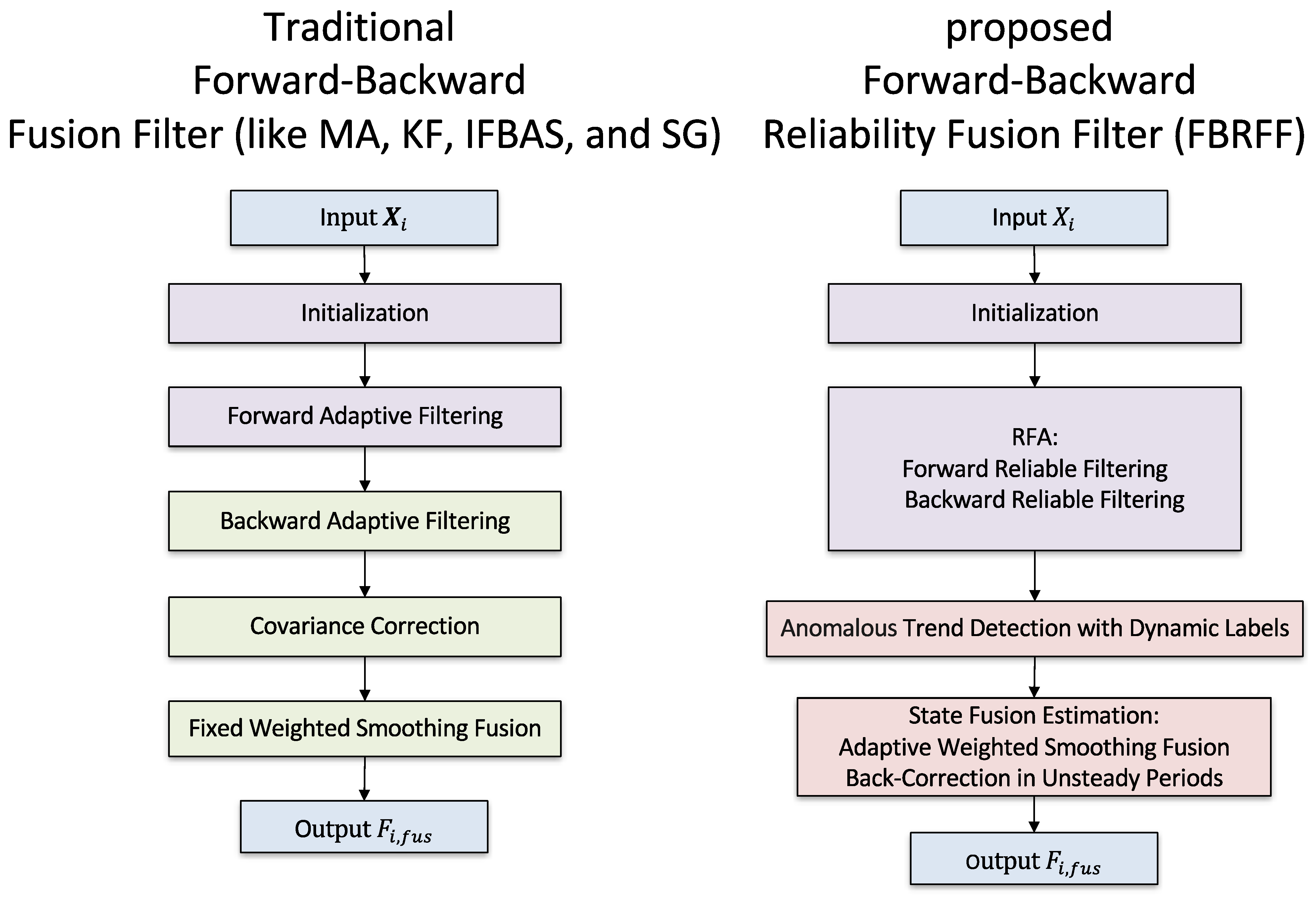
Figure 1 provides a comparative overview of the architectural flow between conventional forward–backward fusion filters—such as Moving Average (MA), Kalman Filtering (KF), the Improved Forward–Backward Adaptive Smoothing (IFBAS), and Savitzky–Golay (SG) algorithm—and the proposed Forward–Backward Reliability Fusion Filter (FBRFF). MA, KF, or other fixed-smoothing models typically adopt a unidirectional processing structure, where data are filtered in a forward-only sequence. The SG filter, while capable of preserving local polynomial trends, applies symmetric window-based smoothing without adaptive mechanisms, making it vulnerable to performance degradation in the presence of non-stationary or high-amplitude noise. IFBAS represents an advancement over such simple models by introducing both forward and backward filtering stages and incorporating adaptive variance estimation to improve smoothing performance. However, IFBAS still relies on static fusion weights and symmetric noise assumptions, which tend to be ineffective in handling asymmetric or long-term trend-like noise. In contrast, the proposed FBRFF framework comprises four main functional modules: initialization, reliable filtering (RFA)—which includes forward reliable filtering (FRFA) and backward reliable filtering (BRFA)—anomalous trend detection, and state fusion. These components are integrated within a sliding window architecture to enable real-time, lightweight processing suitable for edge computing platforms.

The initialization module is responsible for pre-allocating memory structures, setting default values for key parameters, and loading recent data sequences to establish the baseline state for filtering. It also performs statistical initialization such as estimating local signal variance, which serves as the reference for trend labeling and confidence gain modulation in subsequent steps. This ensures that the system can operate stably from the first sliding window, even in the presence of initial noise bursts or missing data.

The reliable filtering (RFA) module draws foundational inspiration from the bidirectional framework of IFBAS but incorporates several key enhancements to improve robustness and adaptivity under complex GNSS disturbance conditions. FRFA performs real-time recursive estimation using a lightweight, model-free structure to effectively suppress local outliers and short-term high-frequency noise. In parallel, BRFA operates on reversed temporal sequences, leveraging future observations to refine current state estimates and correct pseudo-displacement trends. This backward process plays a critical role in addressing long-duration asymmetric noise patterns and correcting accumulated directional biases that forward-only filters typically fail to capture. The bidirectional design enables the system to respond not only to immediate anomalies but also to slow-varying drift effects. Theoretically, omitting the backward pass would significantly degrade the algorithm’s ability to differentiate between real displacements and persistent pseudo-signals, particularly under low-SNR conditions. Therefore, the BRFA component is essential to long-term robustness and temporal stability.

To overcome the limitations of conventional smoothing methods, FBRFF integrates two additional algorithmic innovations:

(1) Dynamic Trend Labeling Module:

FBRFF incorporates a dedicated trend anomaly detection mechanism, which adaptively labels segments of the GNSS time series based on both the directional consistency and amplitude magnitude of observed deviations. This module is grounded in the need to reduce false alarms and avoid overcorrection—challenges that plague conventional filters relying on uniform smoothing across all signal phases. Without such discrimination, slow-moving true displacements may be erroneously suppressed as noise, while impulsive anomalies may propagate unchecked. The trend labeling strategy allows the system to conditionally modulate its correction behavior based on local signal context, enabling targeted suppression of pseudo-anomalies while preserving true deformation trends. This selective adaptivity is particularly critical in GNSS applications, where signal irregularities often stem from complex, non-stationary environments. The absence of this mechanism would force the filter to treat all deviations equally, leading to either insufficient filtering or excessive smoothing, both of which compromise monitoring accuracy.

(2) Confidence-Driven Fusion with Backward Correction:

To enhance adaptability during the state fusion stage, FBRFF replaces fixed-weight fusion with a confidence-driven gain modulation mechanism, which performs weighted integration of the forward and backward filtering results for each segment based on the estimated reliability of local trend patterns. This process enables adaptive smoothing intensity within the sliding window, particularly strengthening the correction in non-stationary intervals where uncertainty is high. Inspired by probabilistic trust modeling and robust statistical estimation theory, this design ensures that segments with higher inferred anomaly likelihoods receive proportionally greater correction. Furthermore, in non-stationary phases identified by the trend labeling module, a backward correction mechanism is triggered. Refined state estimates in these windows are then used to overwrite the corresponding raw observations, effectively eliminating cumulative drift and stabilizing future updates.

This joint mechanism improves the algorithm’s responsiveness to transient changes and suppresses asymmetrically biased fluctuations without compromising long-term trend fidelity. In essence, it achieves a principled balance between filtering strength and structural preservation, making FBRFF resilient to noise complexity while preserving critical displacement information for real-time deformation monitoring.

3.3. Reliable Filtering Algorithm Based on Sliding Window

Upon entering the FBRFF framework, the GNSS time series data are first processed by the Initialization Module, which performs normalization, window partitioning, and noise baseline estimation. This step ensures that the input data is temporally aligned and preconditioned for recursive filtering. The processed sequence is then forwarded to the RFA module as ${\mathbf{W}}_{X|FRFA}$ and ${\mathbf{W}}_{X|BRFA}$, which are used for the forward and backward processing steps in the RFA module, which have a window size of w.

The RFA module receives the preprocessed observation sequence ${\mathbf{W}}_{X|FRFA}$ and ${\mathbf{W}}_{X|BRFA}$, and applies bidirectional recursive filtering to generate a pair of directionally refined state estimates: the forward estimate $X_{upd|FRFA}$ and the backward estimate $X_{upd|BRFA}$. These outputs serve as the foundation for subsequent trend detection and confidence-adaptive fusion. The detailed filtering workflow is illustrated in Algorithm 1.

Algorithm 1: Reliable filtering algorithm (RFA) based on sliding window.

3.4. Dynamic Trend Labeling Strategy for Anomalous Trend Detection

The proposed dynamic trend labeling strategy aims to effectively detect anomalous trends in time series data, especially in real-time monitoring scenarios. This strategy is integrated into the Forward–Backward Reliability Fusion Filter (FBRFF), utilizing two main input datasets: $X_{upd|FRFA}$ and $X_{upd|BRFA}$. The core idea is to analyze trend dynamics using a sliding window, dividing the data cycle into stable and unstable trends, thereby providing a mechanism for effective anomaly detection.

3.4.1. Meaning of Trend Labels

Within the sliding window, the trend label $f_t$ at time t indicates the system status as follows:

• $f_t=ST$: The system is in a stable fluctuation state, indicating no abnormal behavior.
• $f_t=UN$: The system is in an unstable upward trend, possibly indicating an upward anomaly.
• $f_t=DN$: The system is in an unstable downward trend, possibly indicating a downward anomaly.
• $f_t=NECE$: The unstable trend has ended, and the current stable trend confirms it was a high-amplitude anomaly.
• $f_t=NECN$: The unstable trend has ended, and the current stable trend suggests it was due to actual displacement.

3.4.2. Mutation Detection and Trend Labeling

The strategy extracts subsequences $Z_{head|FRFA}$, $Z_{tail|FRFA}$, and $Z_{tail|BRFA}$, each containing m data points, from $X_{upd|FRFA}$ and $X_{upd|BRFA}$, for trend analysis. If the data is insufficient for effective analysis, the trend label $f_t$ is set to $ST$ by default.

The initial trend label is determined by the following conditions:

$$f_t=\left\{\begin{array}{cc}ST,\hfill & b_{ht|F}=0or|mea{n}_{h|F}-mea{n}_{t|B}<C|\hfill \\ UN,\hfill & mea{n}_{t|F}-mea{n}_{h|F}\ge C\hfill \\ DN,\hfill & mea{n}_{h|F}-mea{n}_{t|F}\ge C\hfill \end{array}\right.$$

(5)

When the trend is labeled ST, further judgments are made based on the history in the trend label window $W_f$:

When the system is preliminarily labeled as being in a stable trend ($f_t=ST$), it is necessary to incorporate the historical trend information from the trend label sliding window $W_f$ for further determination of potential anomaly transitions. The specific decision rules are as follows:

(a) If both the front-end and back-end trend mutation indicators satisfy $b_{h|F}=b_{t|B}=BN$ (i.e., no significant mutation), and one of the following conditions holds, then set $f_t=NECE$:

• $f_{t-1}=UN$ and $|max\left(X_{upd|BRFA}\right)-mea{n}_{t|B}|\ge C$;
• $f_{t-1}=DN$ and $|mea{n}_{t|B}-min\left(X_{upd|BRFA}\right)|\ge C$.

(b) Otherwise, if the same conditions hold but the difference is less than C, then set $f_t=NECN$.

$mea{n}_{h|F}$, $mea{n}_{t|F}$, and $mea{n}_{t|B}$ are the means of the respective subsequences, and C is the threshold for tolerable fluctuation. $b_{h|F}$, $b_{t|B}$, and $b_{ht|F}$ are the mutation detection results for $Z_{head|FRFA}$, $Z_{tail|BRFA}$, and $Z_{ht|FRFA}$, which are formed by concatenating $Z_{head|FRFA}$ and $Z_{tail|FRFA}$. Mutation detection is performed on these sequences, with the result “$BY$” indicating a sequence mutation and “$BN$” indicating a stable sequence. For a data sequence $X=\{x_1,x_2,\dots ,x_n\}$, the mutation detection formula is as follows:

$$b_X=\left\{\begin{array}{cc}BY,\hfill & |x_n-min\left(X\right)|\ge Cor|x_n-max\left(X\right)|\ge C\hfill \\ BN,\hfill & otherwise\hfill \end{array}\right.$$

(6)

where $min\left(X\right)$ and $max\left(X\right)$ represent the minimum and maximum values of X.

3.5. Confidence-Driven Adaptive Fusion Mechanism

To enhance the stability and interpretability of state estimation under complex GNSS fluctuations, FBRFF incorporates a confidence-driven adaptive fusion mechanism. This mechanism dynamically integrates forward and backward filtering results based on fluctuation status and local confidence levels. The fused state at time step $k\in [1,l]$ is defined as follows:

$$x_{k,\mathrm{fus}}=\left({\gamma }_k·x_{k,\mathrm{upd}|F}+(1-{\gamma }_k)·x_{k,\mathrm{upd}|B}\right)·{\kappa }_k$$

(7)

where $x_{k,\mathrm{upd}|F}$ and $x_{k,\mathrm{upd}|B}$ denote the forward and backward filtering estimates, respectively; ${\gamma }_k\in \{0,1\}$ is the directional fusion coefficient; and ${\kappa }_k$ is a confidence-adjusted gain factor.

3.5.1. Confidence-Guided Gain Adjustment

During uncorrected unsteady phases, the gain factor remains fixed:

$${\kappa }_k=1$$

(8)

Once correction is activated, the gain factor is updated as follows:

$${\kappa }_k={\displaystyle \frac{x_{\mathrm{ref}}}{x_{k,\mathrm{fus}}}}·(1-c_k)+c_k$$

(9)

where $x_{\mathrm{ref}}$ is the reference state (e.g., average during stable periods), and $c_k\in [0,1]$ is the local confidence coefficient defined as follows:

$$c_k=\left|{\displaystyle \frac{D}{x_{\mathrm{turning}}-x_{\mathrm{ref}}}}\right|$$

(10)

where $x_{\mathrm{turning}}$ denotes the local peak estimate before correction, and D is a domain-specific fluctuation threshold.

3.5.2. Directional Fusion Coefficient Assignment

The value of ${\gamma }_k$ is determined by the fluctuation label $f_k$ and correction status $f_l$:

• Stable state ($f_k=ST$):

  $${\gamma }_k=1$$
• Unsteady deviation (upward/downward):

  -

  No correction ($f_l\notin \{\mathrm{NECE},\mathrm{NECN}\}$): ${\gamma }_k=0$

  -

  Pseudo-anomaly correction ($f_l=\mathrm{NECE}$):

  $${\gamma }_k=\left\{\begin{array}{cc}1,\hfill & \mathrm{if}(x_{k,\mathrm{upd}|F}\le x_{k,\mathrm{upd}|B})\left(\mathrm{upward}\right)\hfill \\ 1,\hfill & \mathrm{if}(x_{k,\mathrm{upd}|F}\ge x_{k,\mathrm{upd}|B})\left(\mathrm{downward}\right)\hfill \\ 0,\hfill & \mathrm{otherwise}\hfill \end{array}\right.$$

  (11)

  -

  True displacement confirmation ($f_l=\mathrm{NECN}$): ${\gamma }_k=0$

This confidence-aware fusion strategy enables the model to prioritize more reliable directional estimates and dynamically suppress pseudo-trends while preserving genuine deformation signals.

4. Experiments and Results

4.1. Experimental Datasets

To evaluate the effectiveness of the proposed FBRFF algorithm under diverse environmental and noise conditions, filtering experiments were conducted using real-world GNSS positioning data collected from monitoring point NJC-03. This dataset was obtained from the “Phase I Monitoring Project of the Usnisa Palace and South Slope in the Nanjing Niushou Mountain Cultural Tourism Zone”, conducted between 16 June 2019 and 15 June 2021. The NJC-03 point is located on a south-facing slope susceptible to displacement risks due to rainfall infiltration, subsurface groundwater fluctuations, and anthropogenic construction activities. GNSS data were continuously recorded at a 1 Hz sampling rate and segmented into minute-level files.

To ensure comprehensive coverage of real-world scenarios, eight representative northward (N) coordinate sequences were extracted, each reflecting a distinct environmental or signal disturbance pattern:

• Data1 (stable baseline): This includes a clean, noise-free reference segment under dry weather and inactive slope conditions.
• Data2 (transient anomaly): This includes short-duration spike-like outliers likely caused by multipath or sensor misalignment.
• Data3 (northward pseudo-drift): This contains sustained high-amplitude noise simulating long-term displacement due to cumulative groundwater effects.
• Data4 (southward pseudo-drift): This shows reversed-direction drift simulating environmental recovery or slow reversal.
• Data5 (unidirectional compound noise): This exhibits low-frequency trend-like noise possibly triggered by prolonged rainfall, mimicking early-stage deformation signals.
• Data6 (bidirectional fluctuation): This contains asymmetric, irregular disturbances resembling construction vibrations or combined anthropogenic–natural effects.
• Data7 (true displacement): This captures a verified slow-moving northward displacement process over several days, with minimal noise.
• Data8 (true displacement + embedded anomaly): This contains a real deformation signal embedded with high-frequency non-stationary disturbances, mimicking rainfall-triggered landslide initiation with noise artifacts.

These datasets collectively span a broad range of operational condition—from stable baselines and transient disturbances to complex long-duration trends and true deformation events—offering a robust and realistic benchmark to evaluate filtering performance under multi-environmental scenarios.

4.2. Experimental Setup

The parameters of the FBRFF algorithm were empirically configured based on prior noise analysis of the NJC-03 dataset. All experiments adopted real-time filtering settings consistent with the original 1 Hz data sampling rate.

Table 2. Experimental parameters of the FBRFF algorithm. Sliding indow size w and step s are in units of data points (1 point = 1 s); thresholds C and D are in meters.

Parameter	Description	Value
w	Sliding window size	7200
s	Sliding window step	60
C	Minor fluctuation threshold	0.05
D	Non-stationary fluctuation threshold	0.10

summarizes the core parameter settings.

Each parameter plays a critical role in influencing the algorithm’s behavior:

• w (sliding window size): This determines the temporal range of data used for smoothing and trend detection. If the window is too small, it may fail to capture the full scope of large-amplitude disturbances, leading to inaccurate filtering and possible misinterpretation of noise as trend. Conversely, if the window is excessively large, the algorithm may over-smooth the signal, suppressing genuine displacement changes and reducing temporal responsiveness.
• s (sliding window step): This controls the number of new data points processed per iteration. Smaller values increase responsiveness but with higher computational load.
• C (minor fluctuation threshold): This is used in the trend labeling module to separate stable and unstable trends. Smaller values make the system more sensitive.
• D (non-stationary fluctuation threshold): This is used for adjusting the confidence-based fusion gain during correction phases. It regulates the strength of adaptive gain changes.

These parameters were selected to strike a balance between accuracy, real-time performance, and robustness across varied disturbance conditions.

To ensure comparative analysis, FBRFF was evaluated alongside several baseline algorithms:

• Moving Average (MA) filtering: Forward (FMA) and backward (BMA) implementations.
• Adaptive Kalman Filtering (AKF): Forward (FAKF) and backward (BAKF) variants.
• Improved Forward–Backward Adaptive Smoothing (IFBAS) [18].
• Savitzky–Golay Filtering (SG).

All algorithms were applied to the same dataset under consistent conditions to enable fair and reproducible performance comparisons.

4.3. Evaluation Metrics

To comprehensively evaluate the effectiveness of the proposed FBRFF framework, we adopt a set of quantitative metrics that jointly assess filtering accuracy, real-time responsiveness, and computational efficiency. These metrics are designed to reflect the practical performance requirements of GNSS-based deformation monitoring systems, especially under edge deployment constraints.

(1) Filtering Accuracy

We employ two widely used error metrics to assess the denoising performance:

• Root Mean Square Error (RMS) is used to measure the standard deviation between the filtered output and the reference signal. It provides a strong indication of the method’s ability to suppress large-amplitude noise components and recover smooth displacement profiles:

  $$\mathrm{RMS}=\sqrt{{\displaystyle \frac{1}{T}}{\displaystyle \sum _{t=1}^T}{\left({\widehat{x}}_t-x_t^{\mathrm{ref}}\right)}^2}$$

  (12)
• Mean Absolute Error (MAE) reflects the average magnitude of deviation between the estimated and reference signals. Compared to RMS, MAE is less sensitive to outliers and provides a robust indication of overall accuracy:

  $$\mathrm{MAE}={\displaystyle \frac{1}{T}}{\displaystyle \sum _{t=1}^T}\left|{\widehat{x}}_t-x_t^{\mathrm{ref}}\right|$$

  (13)

Here, ${\widehat{x}}_t$ denotes the filtered output at time t, and $x_t^{\mathrm{ref}}$ is the corresponding noise-free or smoothed reference trajectory. Both metrics are computed over each test sequence (Data1–Data8) to ensure comprehensive evaluation under diverse noise and signal conditions.

(2) Real-Time Feasibility

To verify the suitability of the proposed method for edge computing applications, we evaluate its runtime characteristics on a Raspberry Pi 4B embedded platform. The following metrics are recorded:

• Average Latency per Window (ms): This measures the time required to process each sliding window and generate output. It directly reflects the algorithm’s responsiveness to new incoming data.
• Peak Memory Usage (MB): This indicates the algorithm’s runtime memory footprint, which is critical for deployment on memory-constrained hardware.

(3) Robustness to Disturbance Types

The algorithm is further evaluated across eight representative GNSS displacement sequences (Data1–Data8), which include diverse disturbance scenarios such as baseline (no anomaly), spike noise, long-duration drift, bidirectional fluctuations, and real displacement with embedded anomalies. This allows us to examine the adaptability and generalization of the filtering framework under varied real-world conditions.

Together, these metrics provide a multi-dimensional evaluation framework, covering both signal fidelity and system-level feasibility for real-time deformation monitoring.

4.4. Filtering Results Comparison

To comprehensively evaluate the filtering performance of the proposed Forward–Backward Confidence Estimation Fusion Filter (FBRFF) under various noise conditions, comparative experiments were conducted against six representative baseline methods: Forward Moving Average (FMA) filter, Backward Moving Average (BMA) filter, Forward Adaptive Kalman Filter (FAKF), Backward Adaptive Kalman Filter (BAKF), Improved Bidirectional Adaptive Smoothing (IFBAS), and Savitzky–Golay (SG) filter. 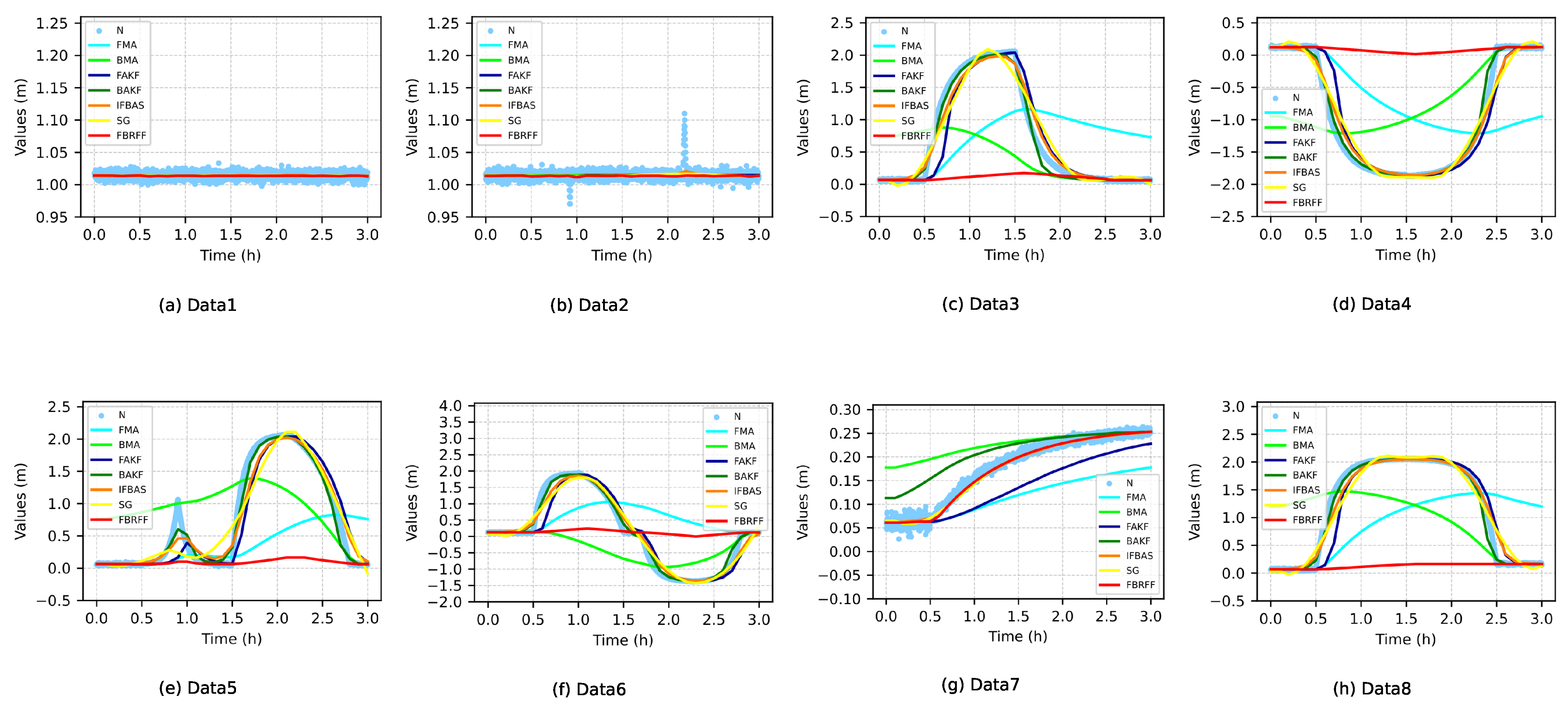Figure 2 presents the filtering results for eight data sequences (Data1 to Data8), which encompass a range of deformation characteristics commonly encountered in GNSS-based landslide monitoring under diverse noise scenarios.

As shown in Figure 2a, under near-ideal noise-free conditions, all methods, including FBRFF, produced comparably smooth outputs. Notably, FBRFF demonstrated superior baseline stability with minimal signal distortion while maintaining the true trend, confirming its robustness and distortion-free filtering capability.

Figure 2b illustrates the scenario with transient spike anomalies. FBRFF exhibited exceptional robustness by completely suppressing all spike outliers and ensuring smooth transitions in the undisturbed segments without introducing oscillations. In contrast, FMA and BMA, lacking adaptive mechanisms, failed to fully eliminate high-amplitude spikes, resulting in noticeable residual distortion. Although FAKF, BAKF, SG, and IFBAS showed improved stability, they still could not thoroughly remove all spike artifacts.

Figure 2c,d demonstrate FBRFF’s superior ability in identifying and mitigating false trends within the sequences. The filtering outputs of FBRFF consistently aligned with the true baseline, effectively resisting long-term low-frequency directional noise. Conversely, FMA and BMA outputs exhibited biased trends, indicating their inadequacy in recognizing and correcting systematic anomalies. While FAKF, BAKF, IFBAS, and SG partially reduced such biases, residual drift or incomplete correction persisted, especially during prolonged interference periods.

In complex interference scenarios depicted in Figure 2e,f, the performance of most baseline methods deteriorated significantly, underscoring FBRFF’s capability to distinguish genuine displacement signals from long-period noise. The majority of baseline filters, including FMA, BMA, FAKF, and BAKF, failed to suppress strong drift components, erroneously following noise-induced patterns that led to severe trajectory distortion. IFBAS and SG filters showed slight improvements but still suffered from trend leakage or oscillatory artifacts. In contrast, FBRFF effectively suppressed both unidirectional and bidirectional disturbances, restoring a stable baseline with minimal deviation. This robustness is crucial in practical monitoring applications, where noise-induced false alarms or misinterpretations could have serious consequences.

Figure 2g highlights FBRFF’s ability to preserve displacement trajectories without delay, attenuation, or distortion, demonstrating outstanding tracking performance. By comparison, FMA and BMA misclassified slow trends as noise, producing overly smoothed outputs that significantly underestimated displacement magnitudes. Although FAKF and BAKF partially tracked trends, they exhibited response delays and endpoint biases. IFBAS and SG maintained relatively accurate trend shapes but showed limited responsiveness at curve inflection points. SG, in particular, failed to preserve full amplitude, resulting in insufficient trend representation near data edges.

Finally, Figure 2h presents the most challenging scenario, where monitoring data contain both long-term high-amplitude anomalies and genuine displacement signals. The FBRFF algorithm uniquely achieved a balanced trade-off between noise suppression and trend preservation, a feat unattainable by the other compared filters.

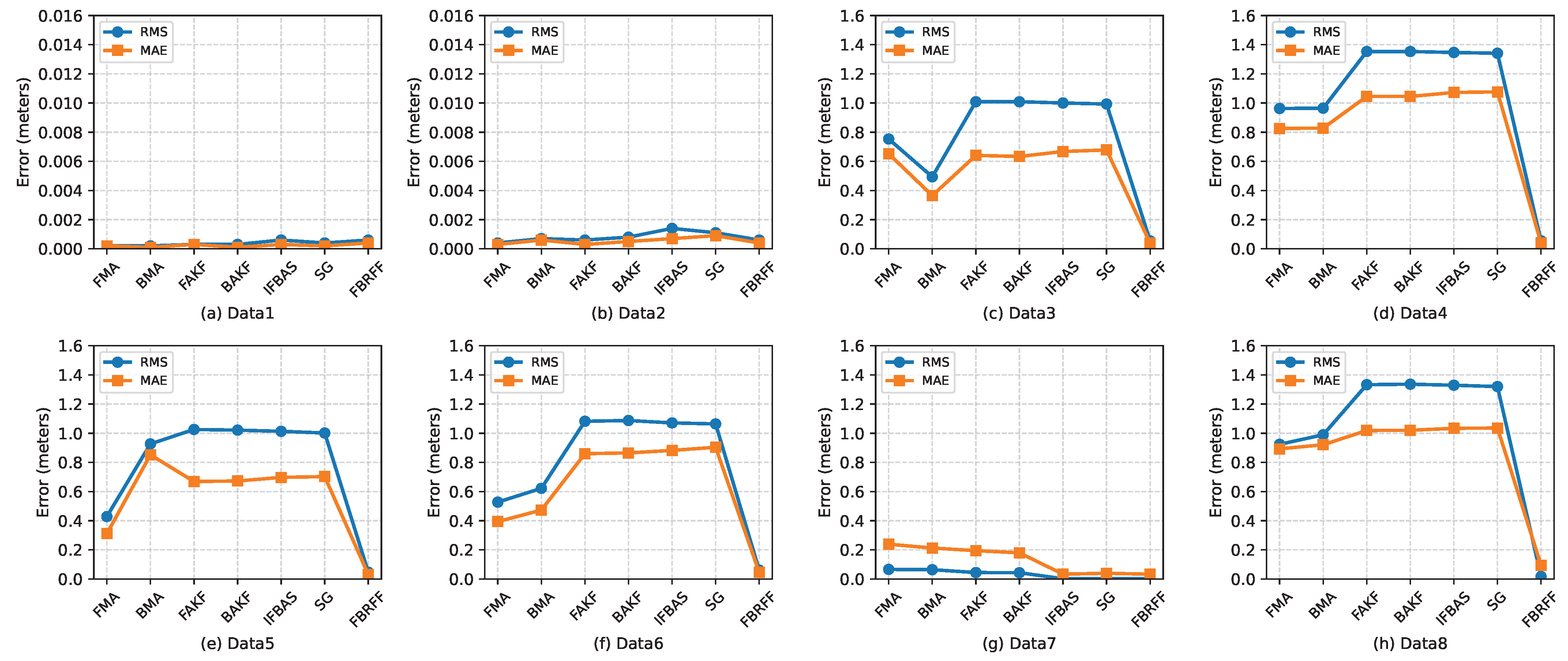
4.5. Filtering Accuracy Analysis

To quantitatively assess the filtering accuracy of the proposed FBRFF algorithm under real-world monitoring conditions, we computed the Root Mean Square Error (RMS) and Mean Absolute Error (MAE) between the filtered outputs and reference trajectories across eight distinct GNSS displacement data sequences. The comparative results are summarized in Figure 3, revealing the accuracy and robustness of each algorithm.

In the noise-free scenario depicted in Figure 3a, all filtering methods produced consistently low error values, with RMS and MAE generally below ${10}^{-3}$ m. FBRFF matched the baseline performance of simple filters like FMA and BMA, achieving RMS and MAE of 0.0006 m and 0.0004 m, respectively. This confirms that FBRFF does not introduce unnecessary smoothing or distortion in ideal conditions, preserving signal fidelity on par with lightweight moving average methods, and thus ensuring its neutrality and precision when no filtering is required.

In the spike anomaly case illustrated in Figure 3b, the FBRFF algorithm achieved a balanced and accurate filtering result, with RMS and MAE values of 0.0006 m and 0.0004 m, respectively. While FMA yielded a slightly lower RMS (0.0004 m), this was primarily due to averaging rather than true spike suppression, and BMA showed higher errors (RMS = 0.0007 m, MAE = 0.0006 m) due to lag effects. FAKF performed competitively (MAE = 0.0003 m) but still left residuals, whereas BAKF introduced further smoothing delays. IFBAS and SG performed notably worse, with RMS exceeding 0.0011 m, reflecting their tendency to overfit or under-constrain the spike anomalies. In contrast, FBRFF effectively suppressed outliers while preserving undisturbed signal segments, avoiding both over-smoothing and oscillation. This demonstrates FBRFF’s robustness in handling short-duration, high-amplitude GNSS noise with superior overall accuracy.

Figure 3c,d depict displacement sequences affected by strong directional disturbances—northward in Data3 and southward in Data4—which often arise from cumulative satellite biases or atmospheric effects. Across both cases, most baseline methods exhibited substantial errors, with RMS values exceeding 1.0 m for FAKF, BAKF, and SG, and similarly elevated MAE levels, reflecting their inability to distinguish false trends from actual displacement. FBRFF, by contrast, delivered consistently low errors in both scenarios, with RMS values of 0.0541 m and 0.0549 m, and MAE values below 0.041 m, achieving over 90% error reduction relative to other methods. This performance highlights FBRFF’s superior trend suppression capability, allowing it to preserve the underlying baseline without being misled by long-period directional anomalies in either direction.

Figure 3e,f present displacement sequences contaminated by complex disturbances— unidirectional in Data5 and bidirectional in Data6—characterized by long-term drifts and frequent polarity reversals, respectively. These types of interference pose significant challenges for conventional filters, as reflected by the high RMS values exceeding 1.0 m across most baseline methods, including FAKF, BAKF, IFBAS, and SG. In contrast, FBRFF maintained robust accuracy, achieving RMS values of 0.0467 m and 0.0607 m, and MAE values of 0.0307 m and 0.0451 m in Data5 and Data6, respectively. These results underscore FBRFF’s strong adaptability to non-stationary and compound noise, enabling it to suppress interference effectively while preserving the core displacement structure in both gradual and rapidly shifting signal environments.

In Figure 3g, the input sequence contains a real, monotonic northward displacement. Here, the challenge is to preserve the actual trend while filtering out noise. FBRFF achieved the lowest RMS (0.0012 m) and MAE (0.0329 m), demonstrating superior fidelity in tracking true motion. Other methods either underestimated the displacement (e.g., FMA, BMA) or introduced endpoint lag (e.g., BAKF, SG). These results highlight FBRFF’s strength in retaining true deformation signals without attenuation or delay, making it well-suited for structural health and geohazard monitoring.

Figure 3h presents the most challenging case, combining genuine displacement with strong embedded anomalies. All baseline methods produced high RMS errors (≥1.32 m), reflecting poor robustness to mixed signal structures. FBRFF, however, maintained a substantially lower RMS of 0.0168 m and MAE of 0.0949 m, indicating its unique ability to simultaneously suppress anomalies and preserve trend integrity. This confirms FBRFF as the only method capable of balancing denoising and fidelity in complex real-world monitoring environments.

4.6. Impact of Key Parameters on FBRFF Performance

This section investigates the influence of the four key parameters—window size w, step size s, minor fluctuation threshold C, and non-stationary threshold D—on the filtering accuracy and responsiveness of FBRFF. In each sensitivity analysis, the parameter under investigation is varied while the remaining parameters are fixed at their optimal configurations as listed in Table 2. This ensures that the observed effects can be attributed primarily to the parameter being analyzed, thereby enhancing the reliability of the evaluation.

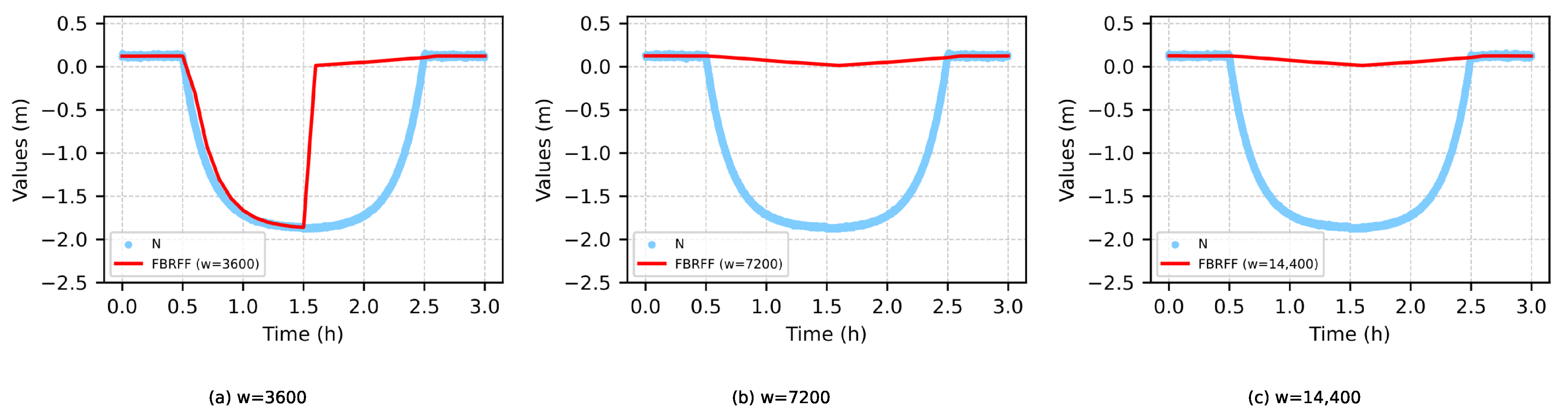
4.6.1. Effect of Sliding Window Size (w)

The sliding window size w dictates the temporal span of historical data employed for filtering and trend labeling. Three configurations were tested: 3600, 7200, and 14,400. As illustrated in Figure 4, when $w<T_{\mathrm{disturbance}}$, the filtering process exhibits partial effectiveness but introduces deviations. Conversely, when $w\ge T_{\mathrm{disturbance}}$, FBRFF accurately classifies the anomaly as a noise event rather than structural displacement, and the performance stabilizes. This phenomenon demonstrates a threshold effect, wherein further increases in w beyond a specific value no longer result in performance improvements.

In practical applications, the window size w should be set to equal or slightly exceed the expected duration of the longest transient disturbance ($T_{\mathrm{disturbance}}$) observed in the monitoring environment. For GNSS-based geohazard monitoring, where pseudo-anomalies caused by multipath or atmospheric effects typically persist from tens of minutes to several hours, a default setting of $w=1–2$ h (e.g., 3600–7200 samples at 1 Hz) is recommended. For environments prone to long-duration noise, such as slow rainfall-induced landslide processes, a larger window (e.g., w = 14,400) may be beneficial, provided that responsiveness requirements are not overly stringent.

4.6.2. Effect of Sliding Window Step (s)

The sliding window step s determines how frequently the window moves and how many new samples are processed per iteration. We evaluated $s=30,60,120$ on Data1 through Data8.

Table 3. Filtering accuracy (Mean Absolute Error) under different s values across datasets Data1–Data8 (unit: meters).

Dataset	$\mathit{s}=30$	$\mathit{s}=60$	$\mathit{s}=120$
Data1	0.039	0.032	0.043
Data2	0.042	0.035	0.051
Data3	0.047	0.038	0.054
Data4	0.045	0.036	0.051
Data5	0.049	0.037	0.055
Data6	0.046	0.034	0.052
Data7	0.043	0.035	0.049
Data8	0.041	0.033	0.048

shows that $s=60$ provides the best balance between responsiveness and computational load. When $s=120$, rapid anomalies were missed due to insufficient temporal resolution. Although $s=30$ offers more frequent updates, no noticeable improvement in accuracy was observed. Moreover, the need to perform anomaly detection on the sliding window at each step led to excessive processing overhead, introducing unnecessary response delays and reducing overall efficiency.

In practical deployments, we recommend setting s to match the expected minimum duration of significant deformation events. For GNSS data sampled at 1 Hz, a step size corresponding to 30–60 s (i.e., $s=30$ to 60) generally provides adequate sensitivity while keeping computational costs low. Applications requiring ultra-low latency or targeting rapid-onset anomalies (e.g., seismic precursor detection) may consider $s=30$, whereas routine structural monitoring with stable patterns may tolerate $s=60$ or higher.

4.6.3. Effect of Minor Fluctuation Threshold (C)

Parameter C is used in trend labeling to identify instability. It determines the minimum deviation considered as a potential anomaly. We evaluated $C=0.02,0.05,0.08$ across Data1–Data8. As shown in

Table 4. Filtering accuracy (Mean Absolute Error) under different C values across datasets Data1–Data8 (unit: meters).

Dataset	$\mathit{C}=0.02$	$\mathit{C}=0.05$	$\mathit{C}=0.08$
Data1	0.044	0.033	0.040
Data2	0.048	0.037	0.042
Data3	0.050	0.038	0.045
Data4	0.057	0.041	0.050
Data5	0.053	0.039	0.047
Data6	0.049	0.036	0.046
Data7	0.045	0.034	0.041
Data8	0.043	0.032	0.040

, $C=0.05$ provides the best trade-off between sensitivity and robustness. Overly small values cause overreaction, while large values overlook subtle shifts.

In practical implementations, C should be tuned according to the intrinsic noise level and displacement scale of the monitoring system. A common approach is to set C at approximately 2–3 times the standard deviation ($\sigma$) of the background GNSS measurement noise, typically in the range of 1–2 cm. For high-precision systems (e.g., RTK or BDS-based GNSS), where baseline noise may be as low as 5 mm, a C value between 0.01 and 0.03 m is recommended for subtle deformation detection. Conversely, for coarser systems or noisy urban deployments, a slightly higher C (e.g., 0.05–0.08 m) helps suppress false positives caused by transient fluctuations or multipath artifacts.

4.6.4. Effect of Non-Stationary Fluctuation Threshold (D)

The parameter D controls the adjustment strength of the fusion gain in unsteady periods. We evaluated $D=0.05,0.10,0.15$ across all datasets.

Table 5. Filtering accuracy (Mean Absolute Error) under different D values across datasets Data1–Data8 (unit: meters).

Dataset	$\mathit{D}=0.02$	$\mathit{D}=0.05$	$\mathit{D}=0.08$
Data1	0.042	0.031	0.039
Data2	0.047	0.036	0.044
Data3	0.051	0.039	0.048
Data4	0.048	0.036	0.044
Data5	0.050	0.038	0.046
Data6	0.046	0.034	0.043
Data7	0.044	0.033	0.041
Data8	0.042	0.031	0.039

shows that $D=0.10$ achieves optimal adaptation without destabilizing the filter. Lower values lead to aggressive but unstable gain adjustments, while higher values reduce correction effectiveness.

In practical deployments, the threshold D should be selected based on the expected amplitude of non-stationary fluctuations and the desired trade-off between responsiveness and stability. When monitoring environments subject to rapid or large transient changes—such as earthquake-prone regions or landslides triggered by intense rainfall—smaller values of D (e.g., 0.05–0.08 m) may be chosen to ensure timely response. In contrast, for systems operating in relatively stable conditions or when false correction must be minimized, a moderate value such as $D=0.10$ is typically ideal. Values exceeding 0.12–0.15 m are only advisable when the deformation scale is large and the noise level is high (e.g., >5 cm variation).

These findings demonstrate that careful tuning of the FBRFF parameters is essential for achieving optimal filtering performance. In practical applications, we recommend initially selecting parameter values based on historical data characteristics and domain-specific monitoring experience, followed by adaptive refinement based on observed signal behavior. Specifically, the sliding window size w should be chosen in relation to the typical duration of expected disturbances; the step size s should reflect the required temporal resolution for timely anomaly detection; and the thresholds C and D should be configured based on the signal’s statistical variance and the anticipated intensity of anomalies.

4.7. Computational Complexity and Real-Time Suitability of FBRFF

To comprehensively evaluate the real-time applicability and practical deployment potential of FBRFF, we conducted a series of systematic experiments focusing on computational efficiency, online stability, and scalability to high-frequency/multi-stream scenarios.

(1) Computational Efficiency on Embedded Devices

To comprehensively evaluate the real-time applicability and practical deployment potential of FBRFF, we conducted a series of systematic experiments focusing on computational efficiency, online stability, and scalability to high-frequency/multi-stream scenarios. Let n denote the number of monitoring epochs and w represent the sliding window size. These operations incur a time complexity of $O\left(w\right)$ per epoch, leading to an overall time complexity of $O(n·w)$. However, thanks to the incremental computation strategies—such as rolling averages and confidence-based updates—the effective per-epoch computational cost approaches constant time, ensuring fast processing speeds suitable for real-time systems. The space complexity is $O\left(w\right)$, relying only on bounded buffers for observations, smoothed states, and trend labels, which ensures that the algorithm remains efficient in terms of memory usage, even when processing long GNSS data sequences.

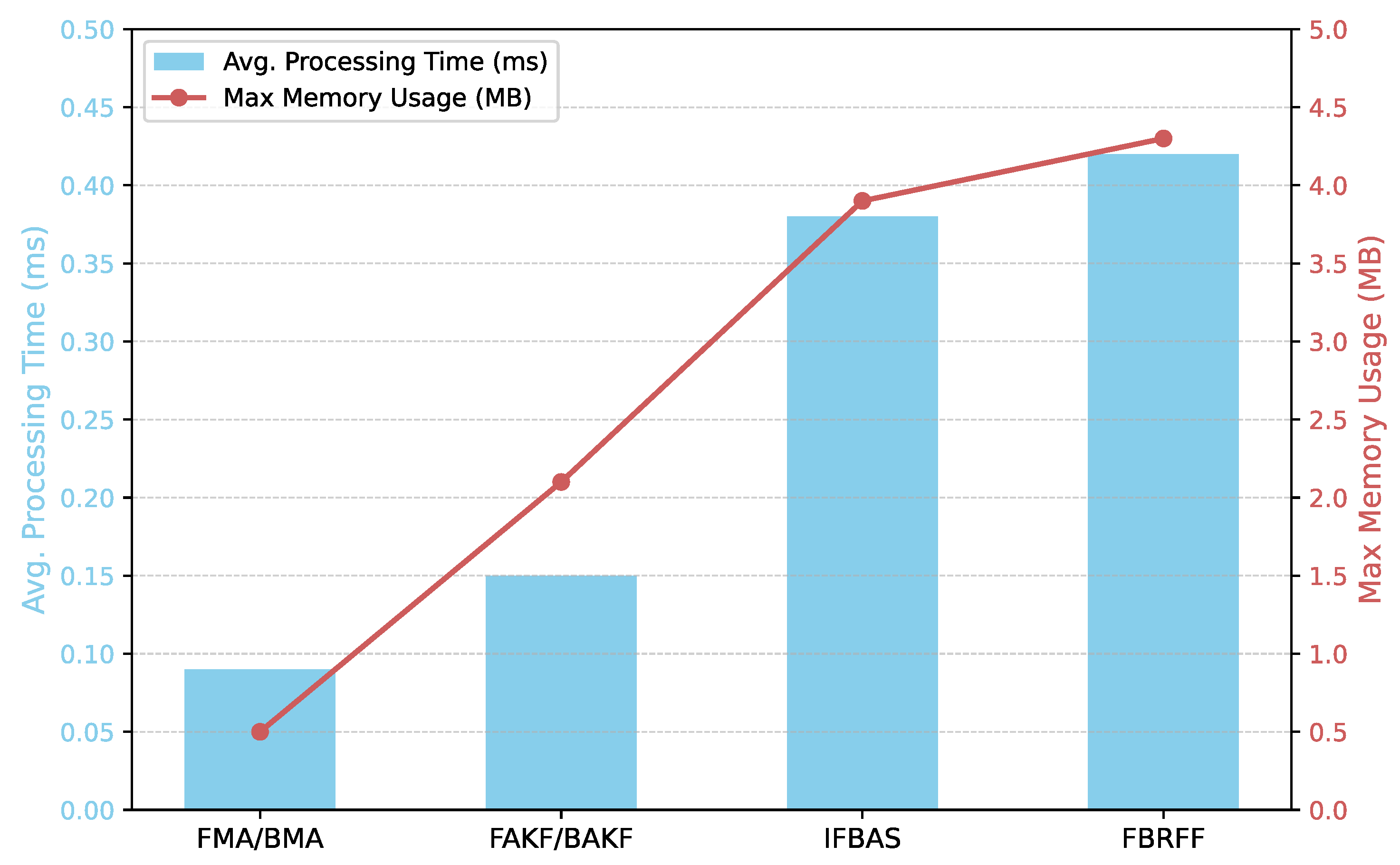
To validate performance under realistic deployment constraints, we benchmarked FMA, BMA, FAKF, BAKF, IFBAS, and FBRFF on a Raspberry Pi 4B (Quad-core ARM Cortex-A72 @ 1.5 GHz, 4 GB RAM; Raspberry Pi Foundation, Cambridge, UK) using 1000 GNSS samples with $w=7200$. Figure 5 summarizes CPU usage and memory footprint for each method.

FBRFF achieves a significant accuracy gain (up to 82%, as shown in Figure 3) while incurring only 1.3× the computational cost of IFBAS. The per-sample average latency remains below 0.5 ms, meeting the 1 Hz GNSS data processing requirement with a sufficient early-warning margin.

FBRFF maintains real-time responsiveness due to three key architectural advantages:

• (1) Parallel forward–backward filtering: This allows partial fusion before full-window convergence.
• (2) Threshold-triggered trend labeling: This enables early decision-making without exhaustive iteration.
• (3) Batch correction for unsteady segments: This distributes the cost of anomaly adaptation over multiple epochs.

(2) Long-Term Online Stability

We further conducted a 24 h uninterrupted real-time filtering test using continuous GNSS data streams. FBRFF maintained stable memory usage and constant update latency, with no buffer overflows or computational delays. Over 86,000 consecutive epochs were processed without performance degradation, demonstrating the method’s suitability for long-term edge deployment.

(3) Scalability to High-Frequency and Multi-Stream Scenarios

To test scalability, we simulated a 5 Hz sampling scenario and parallel processing of three independent GNSS channels. Results show that, with minor parallelization and shared buffer optimization, FBRFF sustains real-time throughput for 15,000+ updates per minute, with CPU utilization below 70% on Raspberry Pi 4B. This indicates that the proposed algorithm remains responsive under high-throughput or multi-sensor conditions, enabling its use in dense GNSS networks and complex deformation fields.

Thus, FBRFF is computationally scalable and suitable for edge devices.

5. Discussion

In this study, the proposed Forward–Backward Reliability Fusion Filter (FBRFF) demonstrated significant advantages in real-time GNSS deformation monitoring, particularly in handling high-amplitude noise and complex disturbances. Experimental results show that FBRFF outperforms traditional methods, such as Moving Average (MA), Adaptive Kalman Filter (AKF), and Improved Forward–Backward Adaptive Smoothing (IFBAS), achieving up to 82% improvement in accuracy, especially in complex unidirectional and bidirectional disturbance scenarios (Data5–6), where traditional methods struggle to maintain stability. The superiority of FBRFF is attributed to its dynamic trend-aware correction mechanism and confidence-based fusion process, which effectively distinguishes true displacement signals from noise, overcoming the limitations of traditional methods in long-duration or asymmetric noise conditions.

When compared to existing GNSS filtering approaches, FBRFF excels in handling long-duration high-amplitude noise and complex dynamic noise patterns. While Kalman Filtering (KF) and its derivatives (e.g., Extended Kalman Filter, EKF) have shown efficacy in dynamic noise filtering, these methods typically assume symmetric and Gaussian noise distributions, which are often violated in real-world scenarios, leading to degraded performance. Machine learning-based models, such as Long Short-Term Memory (LSTM) networks, can adapt to complex noise patterns but require extensive training data and computational resources, making them impractical for real-time edge-based monitoring systems. In contrast, FBRFF offers a low-complexity, real-time solution that does not rely on training data yet still achieves comparable or superior accuracy, demonstrating its practical potential in edge computing environments.

In the experiments, when the dataset was noise-free (e.g., Data1), the performance differences between FBRFF and other algorithms were minimal, confirming that all methods provide reliable results under ideal conditions. However, in more challenging environments, especially in Data7 and Data8, where true displacement is mixed with high-amplitude noise, FBRFF was the only algorithm capable of accurately distinguishing true displacement from noise. Other methods, such as MA and AKF, either over-smoothed the data or misinterpreted the displacement, highlighting the limitations of static-window and fixed-model assumptions when dealing with complex real-world GNSS data.

Unlike traditional Kalman-based filters that rely on predefined process and observation models, the FBRFF algorithm is designed to be model-independent. It does not require prior knowledge of system dynamics or explicit noise covariance matrices. Instead, it adapts to signal behavior through sliding window-based trend analysis and confidence-driven fusion. This characteristic makes FBRFF especially suitable for long-term deployment on edge devices where model updates or environmental re-calibration are impractical. Furthermore, as demonstrated in Section 4.5, its performance remains robust across a variety of noise conditions without the need for parameter retraining or adjustment.

One of the key parameters influencing FBRFF’s performance is the sliding window size. The results indicate that the filtering accuracy is significantly affected by the window size, with optimal performance achieved when the window size matches or slightly exceeds the duration of the dominant disturbances. Smaller window sizes were ineffective in capturing the full scope of large-amplitude disturbances, leading to inaccurate filtering. Conversely, excessively large window sizes led to over-smoothing, suppressed true displacement changes, and reduced temporal responsiveness. These findings suggest a threshold effect in the algorithm’s performance, emphasizing the importance of adjusting the window size according to the target environment’s dominant disturbance duration. In practice, selecting an appropriate window size ensures robustness against long-term anomalies while maintaining responsiveness to legitimate displacements.

The trend-aware correction mechanism introduced in FBRFF represents a significant advancement over traditional filtering approaches. As shown in the experimental results, FBRFF excels in preserving true deformation signals while effectively suppressing pseudo-signals in the presence of long-duration high-amplitude noise. This capability is critical for applications such as landslide monitoring, where early detection of true displacement is essential for timely intervention. By dynamically adjusting the filtering process, FBRFF ensures the preservation of true displacement signals while suppressing non-stationary disturbances, showcasing its robustness in complex environments.

6. Conclusions

In this study, we proposed the Forward–Backward Reliable Filtering (FBRFF) algorithm to address the challenges associated with real-time GNSS-based deformation monitoring, particularly in environments with complex noise, long-duration disturbances, and asymmetric fluctuations. The FBRFF algorithm integrates bidirectional fusion, dynamic trend-aware correction, and confidence-driven adaptive fusion mechanisms, enhancing both the robustness and accuracy of deformation monitoring systems. Experimental results using real-world GNSS data validate that FBRFF not only achieves high filtering accuracy but also maintains real-time responsiveness, even when deployed on resource-constrained embedded platforms such as the Raspberry Pi 4B. In comparison with traditional and state-of-the-art algorithms including IFBAS, FBRFF demonstrates superior performance in terms of both signal fidelity and computational efficiency.

Specifically, FBRFF yields up to 82% improvement in filtering accuracy under high-amplitude disturbance conditions, supports real-time operation with sub-0.5 ms latency per sample and memory usage under 5 MB, and exhibits strong scalability for multi-stream GNSS monitoring at 5 Hz. Furthermore, by deploying the trend-aware correction mechanism directly at the edge terminal, FBRFF enables early-stage detection and suppression of pseudo-anomalies before deformation analysis begins. This on-device pre-filtering effectively reduces system-wide computational burden and operational complexity, particularly in large-scale, multi-source, heterogeneous monitoring networks.

These contributions position FBRFF as a practical and scalable solution for real-time GNSS deformation monitoring in edge computing environments. The algorithm achieves a new balance between computational efficiency and noise resilience, addressing core limitations of existing filtering techniques in handling long-duration and high-amplitude fluctuations. Additionally, its modular and lightweight design facilitates seamless integration with existing monitoring systems and future intelligent filtering frameworks, further enhancing its practical value in real-world geohazard early-warning scenarios.

To ensure applicability across diverse monitoring environments, we emphasize that FBRFF is inherently model-agnostic and does not rely on prior distributional assumptions or training data. The sensitivity analysis of key parameters (w, s, C, and D) presented in Section 4.6 demonstrates that the algorithm maintains stable performance across varied noise types and signal patterns, and that these parameters can be intuitively tuned based on system-specific noise levels and operational constraints. This design choice ensures both configurability and robustness, even when deployed in scenarios with non-Gaussian or evolving noise characteristics.

Nevertheless, this study has certain limitations. Evaluations were based on data from a single static monitoring point, and additional testing under diverse environmental conditions, including highly dynamic or multi-source noise scenarios, is required to further validate the robustness and generalizability of the algorithm. Moreover, certain algorithmic simplifications necessary for real-time performance might limit its ability to capture very subtle deformation trends under extreme conditions.

Building on the limitations identified and the contributions of this study, future research should focus on expanding FBRFF to multi-sensor GNSS networks, incorporating data from diverse geophysical sensors to enhance spatial resolution and improve deformation monitoring accuracy. Developing more adaptive mechanisms that dynamically learn noise patterns from ongoing data streams could further strengthen the algorithm’s robustness, especially in environments with evolving disturbance characteristics. Moreover, long-term field deployments of FBRFF in real-world monitoring scenarios, such as large-scale landslide or earthquake networks, are necessary to comprehensively assess its stability and reliability under varying environmental conditions. By addressing these challenges, FBRFF can be further optimized and extended, making it an even more powerful tool for real-time geohazard monitoring applications.