Data-Driven Prediction Model for Analysis of Sensor Data

Abstract

In view of Industry 4.0, data generation and analysis are challenges. For example, machine health monitoring and remaining useful life prediction use sensor signals, which are difficult to analyze using traditional methods and mathematical techniques. Machine and deep learning algorithms have been used extensively in Industry 4.0 to process sensor signals and improve the accuracy of predictions. Therefore, this paper proposes and validates the data-driven prediction model to analyze sensor data, including in the data transformation phase Principal Component Analysis tested by Fourier Transformation and Wavelet Transformation, and the modeling phase based on machine and deep learning algorithms. The machine learning algorithms used for tests in this research are Random Forest Regression (RFR), Multiple Linear Regression (MLR), and Decision Tree Regression (DTR). For the deep learning comparison, the algorithms are Deep Learning Regression and Convolutional network with LeNet-5 Architecture. The experimental results indicate that the models show promising results in predicting wear values and open the problem to further research, reaching peak values of 92.3% accuracy for the first dataset and 62.4% accuracy for the second dataset.

1. Introduction

Industry 4.0 refers to the fourth industrial revolution, which is characterized by the integration of advanced technologies into various industries. Machine learning (ML), a subset of artificial intelligence, plays a crucial role in this revolution. It enables efficient analysis of large volumes of data, identifying correlations, patterns, and insights that can drive innovation and improve processes across different fields, such as machine health monitoring, quality control, anomaly detection, and others.

Industry 4.0 relies on two main concepts—automation and data [1]—which are interdependent; the development of one correlates to the development of the other and vice versa. Data-driven approaches need huge amounts of data, which are conducted on servers located in data centers or the cloud. Data-driven techniques such as knowledge-based models, life expectancy models, and neural networks can efficiently create behavioral models. However, these methods primarily rely on historical data spanning from a healthy state to a failure state of the system being monitored [2]. This approach increases system complexity and helps with system failure [3]. The development in the field of sensorics and wireless technologies enabled the generation of data for efficient analysis in different industry applications.

Analysis of sensor signals with machine learning is becoming a fundamental part of the optimization of production processes because of the complexity of these signals and the advantages and flexibility of machine and deep learning algorithms. Complex neural network architectures, mathematical transformations, and regularizations enable these algorithms to find correlations and patterns in high-dimensional data.

For many machine learning based on predictive maintenance applications in various industrial processes feature selection represents an important part. The feature selection methods, such as Fisher score, mRMR, and ReliefF, show different results according to the size of the datasets. The stability of all the methods suffered in some cases under the small datasets, but with large datasets, Fisher’s score has the stability and predictive performance in almost all the individual cases [4].

Deep Learning (DL) has become a rapidly developed and researched part of ML. For analysis and processing with large datasets, deep learning algorithms are showing promising results [5,6,7]. Also, it shows excellent performance in different areas, such as object recognition, speech recognition, state prediction, and image segmentation. The benefits of deep learning applications in manufacturing are optimization of operation costs, productivity improvement, fault diagnosis, downtime optimization, and improvement of processes.

To exploit the advantages of these approaches, we propose a data-driven prediction model to analyze sensor data using machine and deep learning algorithms. The data utilized in this study come from a shearing-cutting operation and is collected through sensors located on the press. To validate the proposed model, the test case will be a prediction of different wear conditions of a punch during the stamping process. During operation, the punch of a stamping press is critical to the quality of the produced goods. The wear of the punch plays a crucial role in achieving the desired quality. The conditions are dynamically changing during the process—wear proactively hinders the quality of the product.

Our main contributions can be summarized as follows:

• First, we propose a data-driven model to analyze and extract data and features from the datasets. Using mathematical transformations, such as PCA-Analysis, for dimensionality reduction and optimization. After this optimization, the dataset undergoes Fourier and Wavelet transformations to shift the approach to the dataset without losing data;
• The transformed and optimized datasets are used in ML and DL algorithms for prediction and classification—benchmarking them against each other for comparison;
• The datasets are generated from test benches designed according to real-world standards.

The rest of the paper is organized as follows. Section 2 presents the related works in the application of machine and deep learning in manufacturing as production quality and its optimization. Section 3 describes the proposed data-driven prediction model to analyze sensor data using machine and deep learning algorithms. Section 4 explains the data transformation phase, which includes Principal component analysis, which is tested by Fourier transformation and Wavelet transformation. Section 5 is the modeling phase based on machine and deep learning algorithms, and Section 6 explains the validation phase. In Section 7, the results of method validation are given and discussed. Section 8 is conclusions.

2. Related Works

In this paper, we use sensor signal analysis in order to be able to predict the state of machine health, which can lead to an increase in production quality and optimization. This is linked to two interrelated processes: machine monitoring and anomaly detection. Both processes use different ML and DL models, requiring the combination of many different techniques. For example, the integration of techniques like Pearson correlation coefficient analysis, sequential bidirectional long short-term memory networks, and enhanced remora optimization algorithm introduces a framework used for accurate temperature prediction of the permanent magnet synchronous machine drives [8].

The tool condition monitoring is part of the process of machine monitoring. In the [9] authors discuss how monitoring systems for tool conditions contribute to optimizing machining processes by detecting signs of tool failures and estimating remaining tool life. The paper also highlights the current limitations and blank spots in implementing machine learning, deep learning, and IoT technologies in tool-embedded tool condition monitoring, such as big data handling and generalization of models, as well as latency in cloud computing. Also, the fast and low-cost solution for tool condition monitoring is provided in [10]. The authors used an Arduino node to acquire sound and current consumption signals through low-cost and non-invasive sensors, but again, they built their model through a machine learning node based on a BeagleBoneBlack unit to build the tool wear model using a logistic regression classifier.

In addition, a condition monitoring tool is used for detecting and preventing sudden tool failures [11]. The approach is built on a Discrete Wavelet Transform (DWT) lifting scheme to extract a time-frequency representation of the AE_rms signals and a long short-term memory autoencoder to compress and reconstruct the DWT features. The suggested approach maximizes the utilization of tool life while ensuring the protection of machined parts, leading to reduced machining downtime and costs.

Machine health monitoring is also part of the machine monitoring process and is affected by the improvements in the fields of sensors and the Internet of Things (IoT). The ability to generate cost-effective data and analyze them finds application in the manufacturing industry [12]. By constantly monitoring systems, a vast amount of data can be gathered and analyzed, opening up a new area of exploration [13]. The study offers a comprehensive overview of the use of ML algorithms in the field of electronics and highlights the state-of-the-art advancements in various electronic components.

To predict future health indicators for prognostic and health management purposes, a combination of the long short-term memory model and an attention mechanism is employed in an iterative manner [14]. Moreover, the similarity method is applied to estimate the predicted remaining useful life distribution of the examined sensor-equipped machine based on historical data from multiple sensor-equipped machines’ health indicators. Also, two distinct ML algorithms are used for structural health monitoring—one involving polynomial regression and the other a shallow neural network [15]. Both are supervised methods involving training with certain data and testing with a supplementary subset of data. The two techniques were first optimized for performance in terms of training and testing and then compared in accuracy. The study confirmed the effectiveness of Machine Learning in identifying impacts.

On the other hand, anomaly detection techniques can be applied in machine health monitoring, which are used to identify unusual patterns or outliers that may indicate potential faults, malfunctions, or abnormal behavior in the monitored machines. Anomaly detection is a process that involves identifying data values or sequences that significantly deviate from the majority of other observations, which are considered normal data. A self-supervised learning (SSL) framework for time-series anomaly detection in an Industrial Internet of Things system is proposed, which consists of two augmentation techniques in time-series data that capture two different patterns of original samples before feeding them to the classifier [16]. The classifier uses a one-dimension convolutional neural network to learn the characteristics of normal data.

The combination of DWT with high and low-frequency separation processing and Long Short-Term Memory (LSTM) for anomaly detection is introduced to extract multi-current signal features and detect anomalies based on weight updating the LSTM network [17]. Experiments on real motor bearing faults and permanent magnet synchronous motor stator faults datasets demonstrate the method’s effectiveness in fusing current features and detecting anomalies.

The primary difficulty in identifying temporal anomalies lies in creating models or systems capable of retaining previous encounters or interpreting patterns from extended and intricate time series data. Distinguishing temporal anomalies should not be mistaken for predicting sensor noise problems, as noise fluctuations or sudden changes in signal amplitude or frequency can be effectively addressed using established digital signal processing techniques like Fast Fourier Transform (FFT) and Radon Fourier Transform (RFT) [18].

3. Data-Driven Prediction Model to Analyze Sensor Data

The proposed data-driven prediction model to analyze sensor data using machine and deep learning algorithms is shown in Figure 1. It is based on the Knowledge Discovery in Time Series for Engineering Applications (KDT-EA), which is a process of generating knowledge from all steps of data management while analyzing and processing datasets consisting of time series (e.g., sensor signals). KDT-EA was developed by the Institute for Production Engineering and Forming Machines at the Technical University of Darmstadt, and it is based on the Knowledge Discovery in Databases (KDD) process [19].

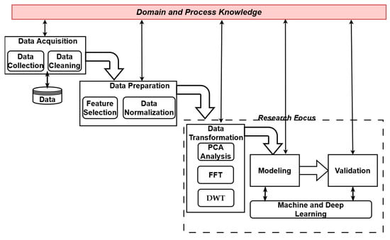
Figure 1. Data-driven prediction model for analysis of sensor data with main phases: Data Acquisition, Data Preparation, Data Transformation, Modeling, and Validation.

The diagram shows the main phases, which include Data Acquisition, Data Preparation, Data Transformation, Modeling, and Validation. Data Acquisition is composed of two processes: data collection and data cleaning to prepare the dataset. The data preparation phase includes feature selection and data normalization. However, the focus of our research is the Data Transformation, Modeling, and Validation phase, where we proposed different solutions, which are described in the following sections.

The data used in this research are from a shear-cutting process and is generated via sensors on the press. The sensors gather force data during the process. Figure 2a,b shows the difference between no wear and critical wear and the different force curves for different wear conditions.

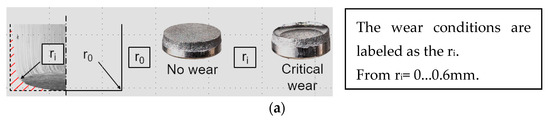
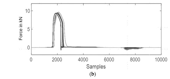
Figure 2. (a) Difference between no wear and critical wear. (b) Difference between force curves for all wear conditions from r_i = 0 to r_i = 0.6 mm., with 0.1 mm steps in-between.

The two datasets are labeled with different wear conditions. Table 1 shows the difference between both datasets.

Table 1. Dataset information.

	First Dataset	Second Dataset
Number of strokes	20	20
Stroke speed	100–500 strokes per minute	100–500 strokes per minute
Wear conditions	0–0.6 mm (0.1 mm steps)	0–0.75 mm (0.05 mm steps)

4. Data Transformation Phase

For Data Transformation Principal Component Analysis (PCA) is used. This is a statistical process that allows the user to analyze large quantities of tabular datasets by smaller fractions of “summary indices”. PCA is the fundamental block of multivariate data analysis based on projection methods. The most important application of PCA is the ability to represent multivariate tabular data as a smaller set, thus easing the observation and detection of trends, jumps, or clusters. This analysis can detect relationships and correlations between observations and variables. The PCA approach allows the analysis of data with missing values, imprecisions or categorical data, making it flexible and with application in various fields. PCA’s goal is to extract the important information from the dataset and to represent it via the smaller indices called principal components.

In statistical terms, Principal Component Analysis finds lines, planes, and hyper-planes in the K-dimensional space, which can approximate the data in the best way. The approximation via a line or a plane for given data points, on the basis of least squares approximation, makes the variance as large as possible.

After the above explained steps, the first principal component (PC1) is ready to be calculated. PC1 is the line in the K-space with the best approximation according to the least squares rule. Each yellow dot in Figure 3 is an observation that can be projected onto this line, thus getting a value along the PC-line.

Figure 3. PCA Visualization and PC1 line in the K-space with the best approximation according to the least squares rule.

The second principal component (PC2) is represented again via a line in the same K-space, and the line is orthogonal to the first PC-line. Passing through the origin (mean value), PC2 helps the approximation.

Data transformation with PCA is performed only after feature extraction using TSFRESH/TSFEL libraries.

4.1. Fourier Transformation

For these tests, a Fourier Transform is performed to achieve better results. The Fourier Transform (FT) is a mathematical transformation that transfers the function from the time domain to the frequency domain. The magnitude of this transform is equal to the amount of presence of a given frequency in the original function. In mathematical terms, the Fourier Transform is explained by the following Equation:

$$\widehat{f}(\omega )=\underset{-\infty }{\overset{\infty }{\int }}f\left(t\right)e^{-j\omega t}dt$$

(1)

• $\widehat{f}$ is the continuous Fourier Transform of the function f;
• $\omega$ is the angular frequency;
• $j$ is the imaginary unit.

Figure 4 shows the difference between them for the force signal used in the tests. The frequency domain graph shows only the first section of the signal (0–200) samples because of scaling issues.

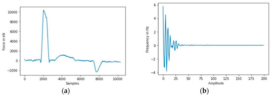
Figure 4. Force curve in (a) time-domain and (b) frequency-domain for the force signal used in the tests.

4.2. Wavelet Transformation

Fourier transformation has a high resolution in the frequency domain, but in the time domain, it has a resolution of zero. Thus, Fourier transformation gives exact information about the frequencies present but no information about the time they occurred. Figure 5 shows the difference between two signals in time and frequency domain.

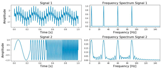
Figure 5. Signals and frequency spectrum of a signal contain four frequencies at all times: four different frequencies at four different times.

As seen, the two frequency spectra contain the exact number of peaks—four—meaning the information after Fourier Transformation is insufficient.

The better approach for analyzing signals with a dynamic frequency spectrum is the Wavelet Transform. This transformation has high resolution in both domains’ frequency and time, giving information not only about the frequencies present but also about the time they have occurred. This is achieved by using and working with different scales. First, the signal is analyzed with large scale and “large” features are extracted, afterwards with smaller scales in order to extract smaller features. Figure 6 shows the comparison between different transformations with the signal in the time domain as a reference. An indication of the size of the features is the scale and orientation of the blocks; as seen, the original time series has high resolution in the time domain but low in the frequency domain. This enables the detection of small features in the time domain and none in the frequency domain. The Fourier Transformation enables the opposite—high resolution in frequency and low in time series. An in-between step is the Short Time Fourier Transformation, which has a medium-sized resolution in both domains.

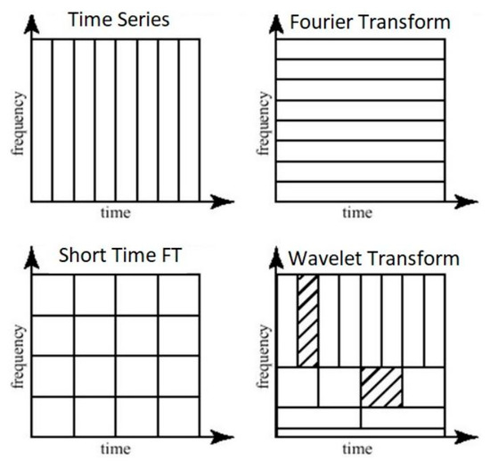
Figure 6. Overview of different transformations in comparison to the original signal in the time domain.

On the contrary, Wavelet Transform offers:

• High resolution for small frequency values in the frequency domain and low resolution in the time domain;
• Low resolution for large frequencies in the frequency domain and high resolution in the time domain.

The Wavelet Transform uses a function called Wavelets. The difference is that Fourier Transformation uses a sine wave that stretches in the interval between − and + infinity, Figure 7. A Wavelet is localized in time.

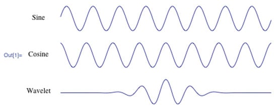
Figure 7. Comparison between a sine-wave, cosine wave and Wavelet.

Because of this localization in time, it is possible to multiply the original signal with the Wavelet at different times. Starting from the beginning of the signal and moving towards the end. This process is called convolution. After the Wavelet transform of the one-dimensional signal, the output is in a two-dimensional form (time-scale) called a scaleogram. The dimension is called scale because the term frequency is reserved for the Fourier Transform. This is the reason behind the two axes of the scaleogram—time and scale. In comparison to Fourier Transform, where only one type of wave is used, there are many types of wavelets that are suited for different signals. Depending on the original signal, one can tailor a wavelet to the needs of the specific situation for best results. Only two mathematical conditions need to be fulfilled, meaning it is relatively easy to generate a completely new wavelet for a particular case. The two mathematical constraints are as follows:

• Finite energy—Localization in time and frequency, integrative, and the inner product between Wavelet and signal always exists;
• Zero mean in time-domain—ensuring it is integrative and the inverse of the Wavelet transform can be calculated.

5. Modeling Phase

In recent years, the collection of data for important variables over time has been a critical aspect in the progress of smart manufacturing systems, which are made possible through the invaluable contribution of sensors [20]. The experimental framework adopts DL algorithms to categorize Multivariate Time-Series data as either failure/unusual events or regular events. To address the issue of imbalanced data, data balancing techniques such as ensemble learning with undersampling and synthetic minority oversampling techniques were employed. Furthermore, along with DL algorithms like Convolutional Neural Network (CNN) and LSTM, ML algorithms like Support Vector Machine (SVM) and K-nearest neighbor (KNN) were also employed. The findings indicate that CNN is potentially the most effective algorithm for accurately classifying this dataset into two categories, and it outperforms both traditional approaches and other deep learning algorithms [20].

5.1. Traditional Machine Learning Algorithms

The first test, as a benchmark for future reference, is the traditional machine learning algorithms for regression and classification. The results will be used as baselines for comparison between shallow and deep learning. The tests will be separated into two categories—the first dataset and the second dataset. The data used for both cases are the output data from the TSFRESH library. The TSFRESH library extracts features from a given time series, such as the absolute energy of the time series and the highest value of the time series—maximum, mean change, median, and variance.

After the extraction, a correlation analysis is performed. The correlation analysis is performed in four steps, as seen below:

• Feature extraction;
• Calculation of Pearson’s correlation coefficient for each feature with the wear radius;
• Sorting of correlation coefficients;
• Using n strongest correlating features for tests;

The algorithms used for regression tests are Random Forest Regression (RFR), Multiple Linear Regression (MLR), and Decision Tree Regression (DTR).

5.2. Deep Learning Regression Model

The structure of the Deep Learning Regression Model is constant for all test cases, meaning it performs well for the whole range of features 1 − 500. The architecture is shown in Table 2.

Table 2. Deep Learning regression model architecture.

Name of Layer	Number of Neurons
Input layer	16
Hidden Layer 1	32
Hidden Layer 2	16
Hidden Layer 3	32
Hidden Layer 4	16
Output layer	1

5.3. Convolutional Neural Network with Wavelet Transform

The advantage of a Convolutional Neural Network (CNN) lies in the ability and efficiency to learn characteristic patterns of labels in images. This type of network can also analyze the two-dimensional CWT coefficients as pixels of an image.

In addition, all coefficient matrices are resized to a squared shape (64 × 64). This step is used because of the different lengths of the signal depending on the hub speed of the press, and CNN works with constant input shapes in Figure 8a,b. The chosen architecture is the LeNet-5 architecture in Figure 9.

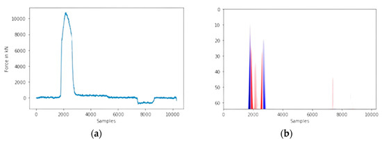
Figure 8. (a) Force curve in time domain; (b) scaleogram of force curve.

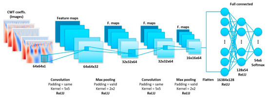
Figure 9. CNN Architecture (LeNet-5).

6. Validation Phase

The coefficient of determination R² is used in statistical models where prediction is the main purpose. It measures the predicted values based on the proportion of total variation of predictions. R² score shows to what degree the variance of one variable explains the variance of the second, in comparison to the correlation coefficient, which indicates the strength of the relationship between independent and dependent variables. For example, an R² score of 0.50 shows that half of the observed variation can be explained by the model’s inputs. The interval of this score is [0:1]. The general mathematical definition of the R² score is as follows:

$$R^2=1-\frac{S{S}_{res}}{S{S}_{tot}}$$

(2)

• $S{S}_{tot}={\sum }_i{\left(y_i-\overline{y}\right)}^2$—Total sum of squares (proportional to the variance of the data), where $y_i$ is each individual score and $\overline{y}$ is the mean of all scores;
• $S{S}_{res}={\sum }_i{\left(y_i-f_i\right)}^2$—Residual sum of squares, where $y_i$ is each individual score and $f_i$ is the predicted value.

Another criterion on which we measure the performance of a regression model is the Mean Squared Error (MSE). It measures the average of the squares of the error between the predicted and actual values. For predictions, MSE’s mathematical expression is as follows:

$$MSE=\frac{1}{n}\sum _{i=1}^n{\left(Y_i-\widehat{Y}\right)}^2$$

(3)

• $Y_i$—Vector of actual values;
• $\widehat{Y}$—Vector of predicted values.

7. Results and Discussion

7.1. Traditional Machine Learning Algorithms—Regression

Shallow learning algorithms show promising results on the first dataset, with the R² score being in the interval of [0,91:0,99] in Table 3. All algorithms tend to achieve better results with a higher number of features extracted, with the drawback of hardware limitations after 50 features. The same trend goes on for the mean squared error (MSE) where a constant decline is observed with the increase of features selected for the test.

Table 3. R²—Score of Regression Models (left) and MSE of Regression Models (right) (first dataset).

Number of Features	RFR	MLR	DTR	Number of Features	RFR	MLR	DTR
1	0.94678	0.91769	0.92362	1	0.03948	0.0394	0.0394
3	0.97839	0.922453	0.9703	3	0.00209	0.00323	0.003
5	0.98421	0.94665	0.97242	5	0.00085	0.00305	0.00117
10	0.99518	0.97916	0.99576	10	0.00059	0.00131	0.00135
15	0.99839	0.99365	0.99576	15	0.00007	0.00027	0.00008
20	0.99839	0.9941	0.99788	20	0.00007	0.00024	0.0008
25	0.9986	0.99465	0.99788	25	0.00007	0.00023	0.00017
50	0.99811	0.9975	0.99788	50	0.00008	0.0001	0.00008

The second dataset is proven to be difficult to learn for the classification test case in Table 4, but the regression algorithms are performing comparably to the ones on the first dataset. The R² score and MSE are in marginally the same intervals as for the first dataset, meaning shallow learning algorithms perform well on both datasets.

Table 4. R²—Score of Regression Models (left) and MSE of Regression Models (right) (second dataset).

Number of Features	RFR	MLR	DTR	Number of Features	RFR	MLR	DTR
1	0.94863	0.9153	0.93368	1	0.0026	0.00426	0.00333
3	0.94836	0.91921	0.93368	3	0.0026	0.00406	0.00333
5	0.99338	0.93694	0.99171	5	0.00033	0.00317	0.0042
10	0.99644	0.97341	0.99585	10	0.0018	0.00134	0.00021
15	0.99834	0.97884	0.99834	15	0.00008	0.00106	0.00008
20	0.99848	0.98161	0.99751	20	0.00008	0.00092	0.00013
25	0.99745	0.98135	0.99309	25	0.00013	0.00094	0.00035
50	0.99858	0.99537	0.99641	50	0.00007	0.00023	0.00018

7.2. Deep Learning Model—Regression

Deep learning models have the advantage of being able to analyze larger datasets in comparison to traditional machine learning algorithms. For this case, the regression model is able to handle data from all sensors without losing the ability to learn efficiently. As seen from Table 5 and Table 6, the R² score of the regression model is between 0, 95 and 0, 99.

Table 5. MSE and R²—Score of Deep Learning Regression Model (first dataset).

Number of Features	MSE	R2-Score
2	0.00964	0.74599
3	0.00179	0.95286
5	0.00223	0.74129
10	0.00062	0.98343
15	0.00044	0.98830
20	0.00069	0.98186
25	0.00043	0.99370
100	0.00041	0.98917
200	0.00041	0.98932
300	0.00051	0.98663
500	0.00051	0.98663

Table 6. MSE and R²—Score of Deep Learning Regression Model (second dataset).

Number of Features	MSE	R2-Score
2	0.02918	0.40860
3	0.02565	0.48017
5	0.00162	0.96714
10	0.00451	0.90859
15	0.00089	0.98809
20	0.00074	0.98505
25	0.01250	0.74673
100	0.01185	0.75983
200	0.00020	0.99585
300	0.00072	0.98536
500	0.00662	0.86577

7.3. Convolutional Neural Network with Wavelet Transform

Convolutional neural networks (CNN) excel in the ability to extract features from images. This advantage over other neural networks is utilized in these tests. Table 7 shows the architecture used for both datasets.

Table 7. Architecture of 2-D CNN Classification Model with Wavelet Transform.

Layer Type	Output Shape	Number of Parameters
Convolutional layer	(64, 64, 32)	160
Max Pooling 2D layer	(32, 32, 32)	0
Convolutional layer	(32, 32, 64)	2112
Max Pooling 2D layer	(16, 16, 64)	0
Flatten	16,384	0
Fully-connected layer	128	2,097,290
Fully-connected layer	54	6966
Fully-connected layer	6	330

This approach shows promising results in the field of classification. Figure 10 and Figure 11 show the training process. The data are split 70/30 between training and testing. The hyperparameters were chosen empirically.

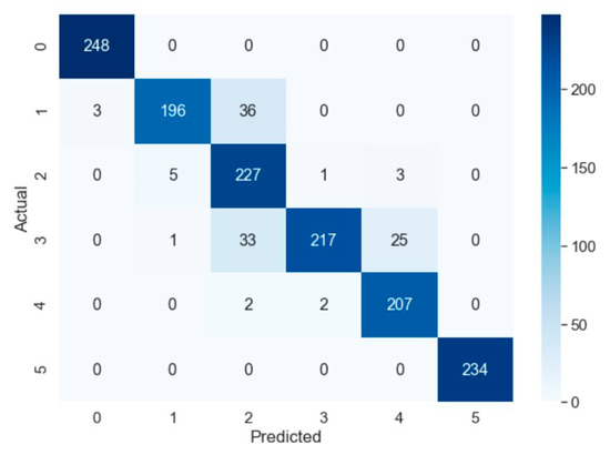
Figure 10. Confusion Matrix of CNN-Wavelet Model (first dataset).

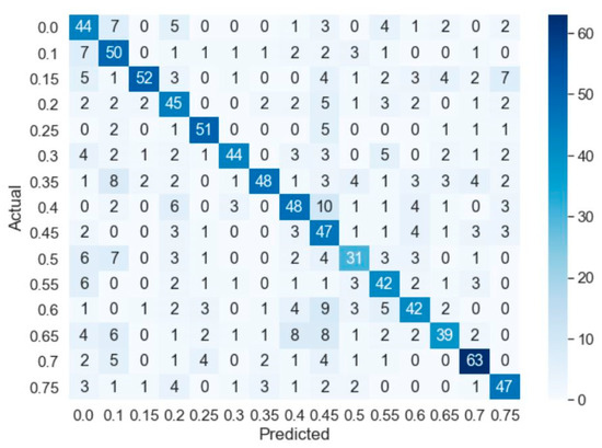
Figure 11. Confusion Matrix of CNN-Wavelet Model (second dataset).

This architecture, with a combination of hyperparameters, showed the best results despite requiring higher computation power. The ability to analyze big datasets and extract features efficiently enabled the CNN to achieve promising results. The accuracy of the trained model is 92.3% for the first dataset with six different wear conditions.

The second dataset is more complex than the first because of the number of different wear conditions, in this case, 15. The model shows promising results, achieving 62.4% accuracy across all classes.

8. Conclusions

Having the information on the wear state of the punch will be crucial for the manufacturer, with the approach not only being viable in this isolated case but for all manufacturing processes where mechanical wear occurs. Deep learning models will be benchmark tested against traditional machine learning algorithms in order for a conclusion to be drawn about the prospects of the application of deep learning models in the context of manufacturing and sensor signal processing. The drawback of deep learning and neural networks is the computational power needed for the training process, which, in some cases, compared to traditional machine learning algorithms, is exponentially larger. This balance between accuracy and complexity will be subject to testing during this research.

After all tests are conducted, the prospects of deep learning algorithms in both scenarios—regression and classification are promising. Sensor signals are complex to analyze, and based on the volume of data that need to be analyzed, a different machine-learning approach needs to be chosen. Due to hardware limitations, the number of features and length of data is limited for traditional shallow learning models. However, their advantage lies in their efficiency in terms of computational resource requirements. In cases with large and multidimensional datasets, deep learning algorithms, because of their neural network topologies and mathematical optimizations, excel in detecting patterns and correlations.

The tests show promising results in both regression and classification problems. Sensor signals are difficult to approach and analyze, and with the increase in volume, traditional machine learning algorithms are not achieving satisfactory results. Therefore, deep learning algorithms need to be used. As seen from the results, until a certain volume of data or, in this case, features, are reached, traditional machine learning algorithms excel at predicting and classifying, but once a certain threshold is exceeded, deep learning algorithms are to be preferred. Deep learning models need large datasets in order to “learn” and make better predictions/classifications. The last tests show promising results in terms of classification—92.3% accuracy for the first dataset and 62.4% for the second, despite the complexity of both. The confusion matrix of the second dataset shows that all inaccurate predictions are close to the value, meaning that in a real-world application, the “usable” accuracy of the model is far greater.

This application of deep learning in engineering processes, especially in manufacturing, can be further researched to optimize deep learning architectures. Pattern recognition via convolutional neural networks in the context of sensor signal classification is a field that can yield industry-changing results for the transition to Industry 4.0.

References

- Wan, J.; Tang, S.; Li, D.; Wang, S.; Liu, C.; Abbas, H. A Manufacturing Big Data Solution for Active Preventive Maintenance. IEEE Trans. Ind. Inform. 2017, 13, 2039–2047. [Google Scholar] [CrossRef]
- Soualhi, A.; Lamraoui, M.; Elyousfi, B.; Razik, H. PHM SURVEY: Implementation of prognostic methods for monitoring industrial systems. Energies 2022, 15, 6909. [Google Scholar] [CrossRef]
- Antonini, M.; Pincheira, M.; Vecchio, M.; Antonelli, F. An Adaptable and Unsupervised TinyML Anomaly Detection System for Extreme Industrial Environments. Sensors 2023, 23, 2344. [Google Scholar] [CrossRef] [PubMed]
- Assafo, M.; Städter, J.P.; Meisel, T.; Langendörfer, P. On the Stability and Homogeneous Ensemble of Feature Selection for Predictive Maintenance: A Classification Application for Tool Condition Monitoring in Milling. Sensors 2023, 23, 4461. [Google Scholar] [CrossRef] [PubMed]
- Zhang, Q.; Yang, L.T.; Yan, Z.; Chen, Z.; Li, P. An Efficient Deep Learning Model to Predict Cloud Workload for Industry Informatics. IEEE Trans. Ind. Inform. 2018, 14, 3170–3178. [Google Scholar] [CrossRef]
- Zhang, Q.; Yang, L.T.; Chen, Z.; Li, P. A Tensor-Train Deep Computation Model for Industry Informatics Big Data Feature Learning. IEEE Trans. Ind. Inform. 2018, 14, 3197–3204. [Google Scholar] [CrossRef]
- Ota, K.; Dao, M.S.; Mezaris, V.; de Natale, F.G.B. Deep Learning for Mobile Multimedia. ACM Trans. Multimed. Comput. Commun. Appl. 2017, 13, 1–22. [Google Scholar] [CrossRef]
- Latif, A.; Mehedi, I.M.; Vellingiri, M.T.; Meem, R.J.; Palaniswamy, T. Enhanced Remora Optimization with Deep Learning Model for Intelligent PMSM Drives Temperature Prediction in Electric Vehicles. Axioms 2023, 12, 852. [Google Scholar] [CrossRef]
- Tran, M.-Q.; Doan, H.P.; Vu, V.Q.; Vu, L.T. Machine learning and IoT-based approach for tool condition monitoring: A review and future prospects. Measurment 2023, 207, 112351. [Google Scholar] [CrossRef]
- Failing, J.M.; Abellán-Nebot, J.V.; Benavent Nácher, S.; Rosado Castellano, P.; Romero Subirón, F. A Tool Condition Monitoring System Based on Low-Cost Sensors and an IoT Platform for Rapid Deployment. Processes 2023, 11, 668. [Google Scholar] [CrossRef]
- Hassan, M.; Ahmad, S.; Helmi, A. A Real-Time Deep Machine Learning Approach for Sudden Tool Failure Prediction and Prevention in Machining Processes. Sensors 2023, 23, 3894. [Google Scholar] [CrossRef]
- Wang, J.; Ma, Y.; Zhang, L.; Gao, R.X.; Wu, D. Deep learning for smart manufacturing: Methods and applications. J. Manuf. Syst. 2018, 48, 144–156. [Google Scholar] [CrossRef]
- Bhat, D.; Muench, S.; Roellig, M. Application of Machine Learning Algorithms in Prognostics and Health Monitoring of Electronic Systems: A Review. e-Prime—Adv. Electr. Eng. Electron. Energy 2023, 4, 100166. [Google Scholar] [CrossRef]
- Yan, J.; He, Z.; He, S. A deep learning framework for sensor-equipped machine health indicator construction and remaining useful life prediction. Comput. Ind. Eng. 2022, 172, 108559. [Google Scholar] [CrossRef]
- Dipietrangelo, F.; Nicassio, F.; Scarselli, G. Structural Health Monitoring for impact localization via machine learning. Mech. Syst. Signal Process. 2023, 183, 109621. [Google Scholar] [CrossRef]
- Tran, D.H.; Nguyen, V.L.; Nguyen, H.; Jang, Y.M. Self-supervised learning for time-series anomaly detection in Industrial Internet of Things. Electronics 2022, 11, 2146. [Google Scholar] [CrossRef]
- Tang, M.; Liang, L.; Zheng, Z.; Chen, J.; Chen, D. Anomaly Detection of Permanent Magnet Synchronous Motor Based on Improved DWT-CNN Multi-Current Fusion. Sensors 2024, 24, 2553. [Google Scholar] [CrossRef]
- Chirayil Nandakumar, S.; Mitchell, D.; Erden, M. Anomaly Detection Methods in Autonomous Robotic Missions. Sensors 2024, 24, 1330. [Google Scholar] [CrossRef] [PubMed]
- Kubik, C.; Molitor, D.A.; Becker, M.; Groche, P. Knowledge Discovery in Engineering Applications Using Machine Learning Techniques. J. Manuf. Sci. Eng. 2022, 144, 091003. [Google Scholar] [CrossRef]
- Rahman, M.M.; Farahani, M.A.; Wuest, T. Multivariate Time-Series Classification of Critical Events from Industrial Drying Hopper Operations: A Deep Learning Approach. J. Manuf. Mater. Process. 2023, 7, 164. [Google Scholar] [CrossRef]
Disclaimer/Publisher’s Note: The statements, opinions and data contained in all publications are solely those of the individual author(s) and contributor(s) and not of MDPI and/or the editor(s). MDPI and/or the editor(s) disclaim responsibility for any injury to people or property resulting from any ideas, methods, instructions or products referred to in the content. |
© 2024 by the authors. Licensee MDPI, Basel, Switzerland. This article is an open access article distributed under the terms and conditions of the Creative Commons Attribution (CC BY) license (https://creativecommons.org/licenses/by/4.0/).