Controllable Local Propagation Environment to Maximize the Multiplexing Capability of Massive MIMO Systems

Abstract

The capability of controlling and modifying wireless propagation channels is one of the prerogatives of beyond-5G systems. In this paper, we propose the use of a controllable local propagation environment surrounding the terminals, and analyze its positive effect on the multiplexing capability of massive MIMO systems. In particular, we focus on using a few switched passive elements surrounding each terminal. In this way, the modification of the propagation environment is not realized by means of a single structure, as in reconfigurable intelligent surfaces (RIS), but is achieved by the cooperative work of all the terminals. By employing numerical simulations, we show that the proposed system outperforms its non-reconfigurable counterpart in terms of the number of contemporary connected users. Moreover, the optimized system enables a substantial increase in the minimum received power by the terminals, thus guaranteeing superior channel fairness.

1. Introduction

The multiplexing of data transmission through wireless channels was historically first performed using time division and frequency division techniques; successively, adopting “code division”, which mixed time and frequency [1]. More recently, it has been noticed that it could be possible to code independent information into the “spatial” variation of the fields by means of Multiple Input Multiple Output (MIMO) systems and related techniques. In particular, Multi-User MIMO (MU-MIMO) systems have opened new perspectives in the communications industry [2,3], since these kinds of systems have transformed the multipath property of a complex propagation environment into a resource that could be exploited to transfer a huge amount of information effectively.

In the last decade, the MU-MIMO paradigm has been pushed even further by the concept of “Massive MIMO” (MaMIMO), in which hundreds, if not thousands, of transmitters at the Base Station (BS) are used to communicate with a huge number of terminals [4,5]. This paradigm, in particular, exploits some useful properties of random matrices to perform efficient processing of the signals using linear techniques, delivering performances that are only a fraction smaller than the optimal ones. In particular, it has been demonstrated that the so-called “favorable propagation” conditions [6,7] can occur with a number of terminals K that can be of the order of a third of the number of antennas M at the base station [8]. For these reasons, MaMIMO is considered one of the enabling technologies for current 5G systems.

Unfortunately, the convenient “favorable propagation” conditions may not arise in real systems; as an example, when the users are too close, their proximity may represent a bottleneck for the achievement of the theoretically foreseen performance [9].

For this reason, researchers of MaMIMO systems have tried to improve the results mentioned above further. Beyond-5G and 6G technology are an additional evolution step with respect to 5G and are currently under development. One of the key differences with respect to current 5G systems is a focus on the possibility of modifying and optimizing the propagation environment and modifying the radiators’ characteristics to better suit the characteristics of the channel. For instance, in [10,11,12], the use of large RISs was investigated for the optimization of wireless channel performance. Double RISs were considered in [13,14]. A metasurface MaMIMO antenna was instead proposed in [15,16,17]. Sophisticated beamforming and precoding were studied in [18,19,20]. The use of irregular arrays for MaMIMO systems was discussed in [21,22], and several synthesis algorithms have been proposed in the literature to solve this task effectively [23,24,25,26,27,28]. Another promising approach is the abandoning of the “cell” concept in the so-called cell-free massive MIMO [29,30,31].

In a recent paper, we demonstrated that it is possible to improve the number of terminals K with which the BS can communicate by means of its optimization without increasing the number of antennas M [32]. The mentioned optimization of the propagation channel was realized using a twofold approach: larger antenna arrays, with inter-element distances significantly larger than half-wavelength, were employed. Moreover, effective user scheduling strategies were used to exploit the increased size of the BS array. It is indeed true that this twofold strategy may not be feasible or convenient. In particular, the requirement of a larger BS antenna array may not be compatible with some deployment constraints.

In this paper, we follow a different approach to achieve a similar effect: we will introduce a controllable local propagation environment (CLPE) around the receiving terminals so that the overall propagation channel can be properly reconfigured to allow communication with the maximum possible number of users. The controllable propagation environment we propose is closely located to the transmitting terminals; in this paper, we realize it via employing parasitic elements, using some of the techniques that have been previously proposed for low-cost smart antennas [33,34,35,36]. In particular, these low-cost antennas were proposed for the optimization of the received power in point-to-point connections or for the reduction of the effect of interferences. Instead, the use of parasitic elements will now be focused on the improvement of the multiplexing capability of multiuser systems.

It is worth underlining that the proposed propagation environment modification scheme shares some similarities with the use of RIS mentioned previously. Differently from RISs, which may require large apertures and are usually employed in a limited number in current research activities, we propose the use of smaller structures that are distributed in the overall propagation environment in order to provide a shared optimization of the propagation channel.

In principle, we may also realize a controllable local propagation environment using advanced materials such as graphene [37,38,39], or other more sophisticated switching techniques [40,41]. Some preliminary results on this approach were presented in [42], and in this paper, we discuss the overall paradigm better, as well as present a deeper analysis of the achievable results.

The remainder of this paper is organized as follows. We first recall some of the limiting aspects of the multiplexing capability of MaMIMO systems (Section 2). We then introduce the controllable local propagation environment and its modeling (Section 3), and provide some analyses and results obtained through numerical simulations (Section 4). Lastly, concluding remarks are provided at the end of the paper.

2. Communication System Model

In this section, we will present the employed communication system model that will allow us to emphasize the source of multiplexing limits in MaMIMO systems.

In particular, for the sake of simplicity, we will focus on narrowband MaMIMO systems working at a fixed frequency f and using M radiating elements on the BS and K single-antenna terminals, with $K<M$. For this kind of multi-user system, the channel matrix $\mathbf{H}\in \mathcal{C}(K,M)$ can be written as:

$$\mathbf{H}=\left[\begin{array}{c}{\mathbf{h}}_1\\ {\mathbf{h}}_2\\ ⋮\\ {\mathbf{h}}_k\end{array}\right]$$

(1)

where ${\mathbf{h}}_k$ is a row vector representing the response of the $k-$th terminal to the M antennas of the BS. The aforementioned channel response ${\mathbf{h}}_k$ depends on the architecture of the BS array (element type, orientation, and displacement), as well as the position of the terminal in the propagation environment. In this paper, we will simulate the channel’s response employing an uncorrelated scattering model [43] with a variable distribution of the point scatterers for each channel realization.

In the numerical examples discussed in this paper, we will use the Zero Forcing (ZF) [44] beamforming approach; this choice has been suggested by the relative simplicity of the ZF approach, which requires simple linear processing to perform the multiplexing of the users. Moreover, it has been demonstrated that the ZF approach provides performance close to the optimal one when the channel shows favorable propagation conditions [8].

The calculation of the excitation of the array element will be then performed by preliminarily calculating the pseudo-inverse [45] of the channel matrix $\mathbf{H}$ as

$${\mathbf{H}}^{†}=[{\mathbf{h}}_1^{+}{\mathbf{h}}_2^{+}\cdots {\mathbf{h}}_k^{+}]$$

(2)

where ${\mathbf{h}}_k^{+}$ are the columns of the pseudo-inverse; the excitation vector ${\mathbf{a}}_k$ to communicate with the $k-$th terminal will be then calculated as:

$${\mathbf{a}}_k=\frac{{\mathbf{h}}_k^{+}}{\parallel {\mathbf{h}}_k^{+}{\parallel }_2}$$

(3)

where the normalization with ${\ell }_2$ norm of ${\mathbf{h}}_k^{+}$ is performed to transmit the same power for each terminal.

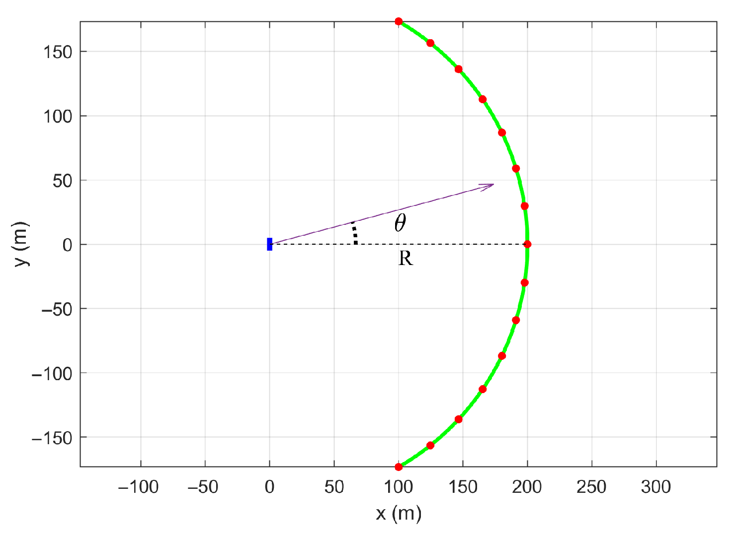
Let us now gain a deeper insight into the signals radiated by a BS antenna when the ZF approach is employed. With reference to Figure 1, we will consider a BS made of $M=50$$\lambda /2$ equispaced elements working at a frequency $f=3.5\mathrm{GHz}$, aligned along the y-axis of a standard Cartesian coordinate system; the $K=15$ antenna terminals, instead, will be placed at a fixed distance $R=200$ m from the BS antenna, in increasing angularly equispaced positions in the range $\theta \in [-\pi /3;+\pi /3]$.

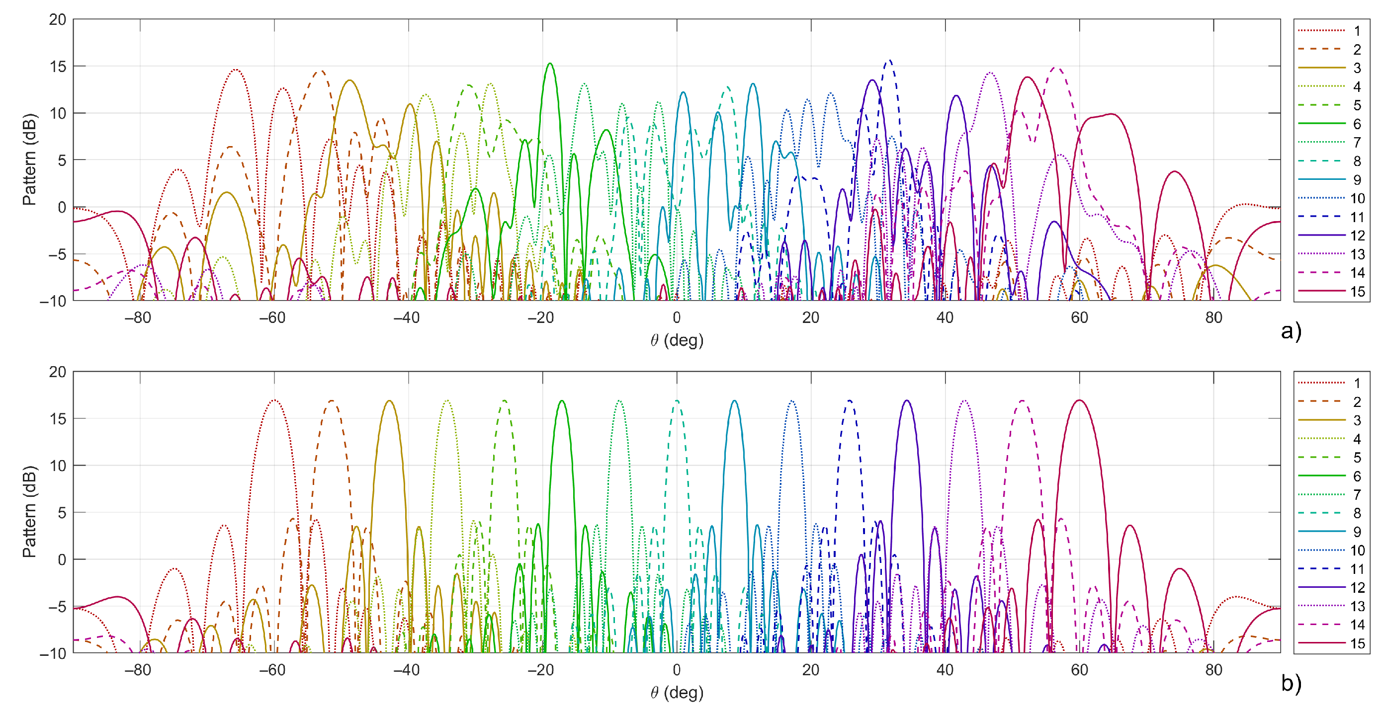
In Figure 2a, we can see the plot of the array factor $A{F}_k$ relative to each one of the $K=15$ excitations ${\mathbf{a}}_k$ for a specific channel realization

$$A{F}_k\left(\theta \right)=\sum _{m=1}^M{a}_k\left(m\right)e^{j\beta y_{m}sin\left(\theta \right)}$$

(4)

where $\beta =2\pi /\lambda$ is the free space wavenumber, $a_k\left(m\right)$ is the $m-$th entry of ${\mathbf{a}}_k$ and $y_m$ is the coordinate of the $m-$th antenna at the BS. These patterns show a very irregular shape that is due to the particular realization of the propagation channel; just for reference, in Figure 2b we provide the same plot for the Line-of-Sight propagation case (with no objects in the environment). This latter plot shows a much more regular behavior.

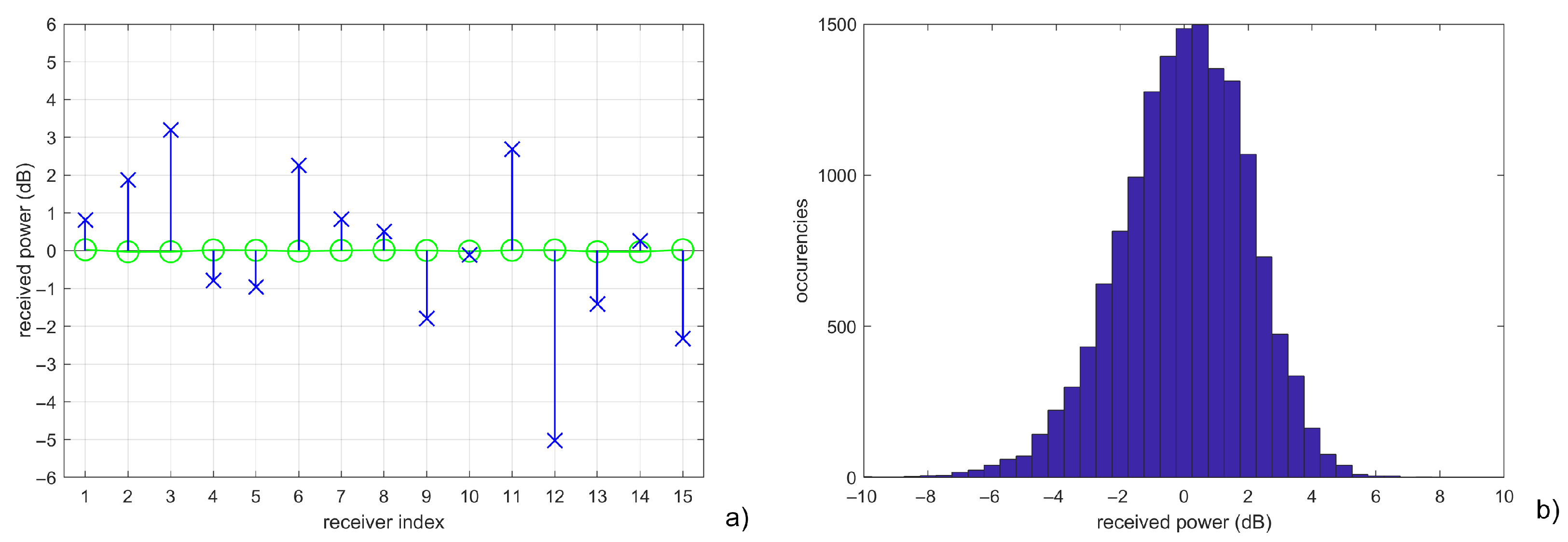
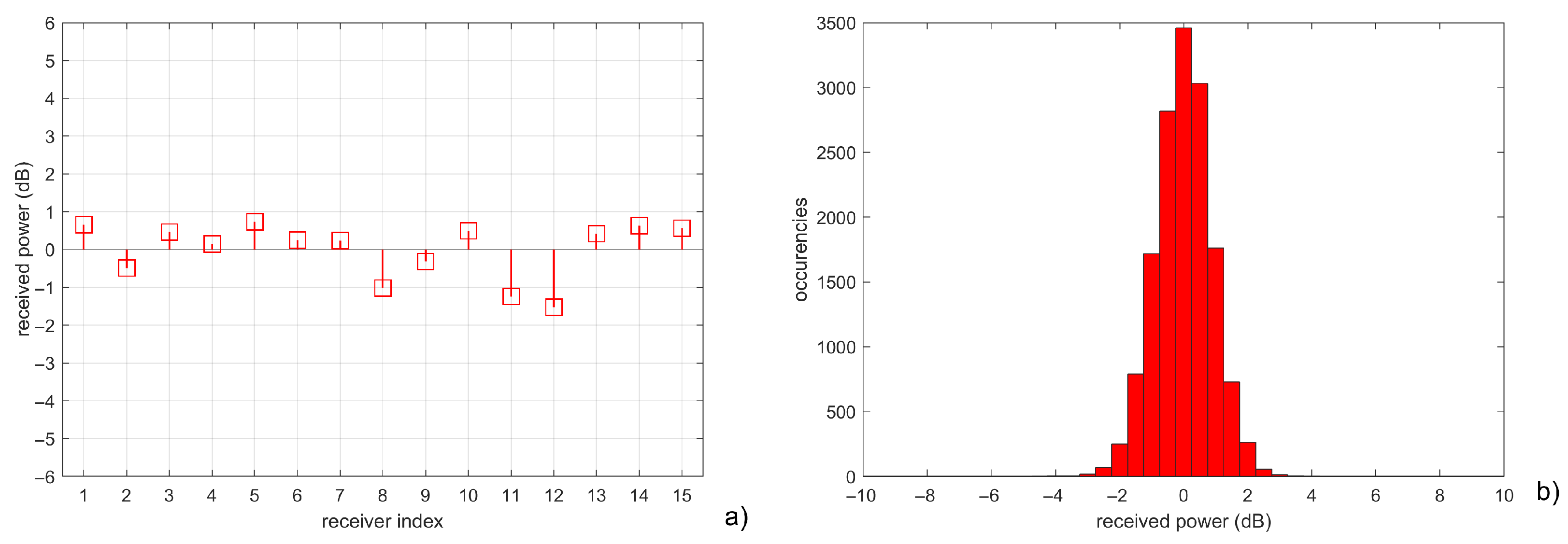
It is now particularly interesting to calculate, for the same channel realization considered above, the values of the received channel powers. In Figure 3a, we can see that the values of the power level received by the K terminals normalized to the average values. While the power in the LOS case is almost constant, the power level for the NLOS case shows variations of some dBs between the users.

Since the distance of the terminals from the BS is the same, the origin of these variations is due to two factors: first, the fading due to the simulated multi-path environment; second, the fact that some terminals show similar propagation channel responses ${\mathbf{h}}_k$, so the zero-forcing solution is unable to focus a sufficient power towards each user. This effect is also understandable from Figure 2; for instance, the pattern relative to $k=12$ shows very low levels in the direction of the terminal, that is placed around $\theta ={34}^{\circ }$(deg).

The effect seen is not due to a particularly unlucky channel realization; if we repeat the same analysis for $P=1000$ different scenarios, we can obtain the power level distribution of Figure 3b, in which the power levels, normalized to the average, show an almost Gaussian behavior, with a standard deviation of ${\sigma }_0=2.01$ dB.

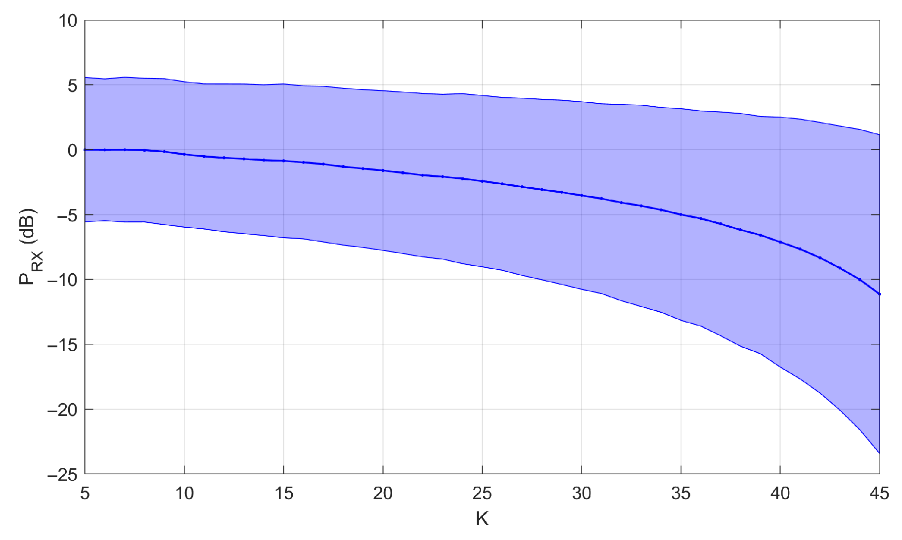
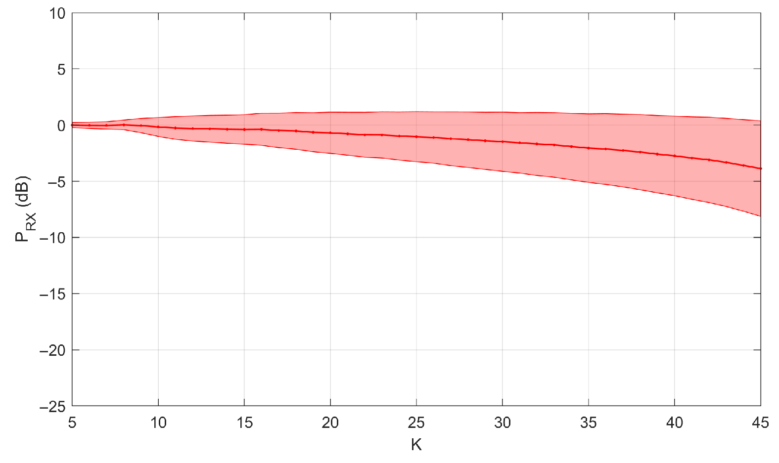
Similarly, we could repeat the same analysis for a variable number of user terminals. In Figure 4, we can see a representation of the received power level with a range of terminals from 5 to 45, always placed at a fixed distance $R=200$ m from the BS in the angular range $\theta \in [-\pi /3;+\pi /3]$. All the powers have been normalized, for the sake of simplicity, to the average power level obtained in the case of $K=5$. The solid blue line in the figure represents the average power level received ${\mu }_0$, while the cyan area denotes the area contained between the curves ${\mu }_0-3{\sigma }_0$ and ${\mu }_0+3{\sigma }_0$.

It is worth noting that increasing the number of terminals significantly influences the average level of received power, but results in a dramatic decrease in the minimum power level, making communication with some terminals inconvenient, if not infeasible.

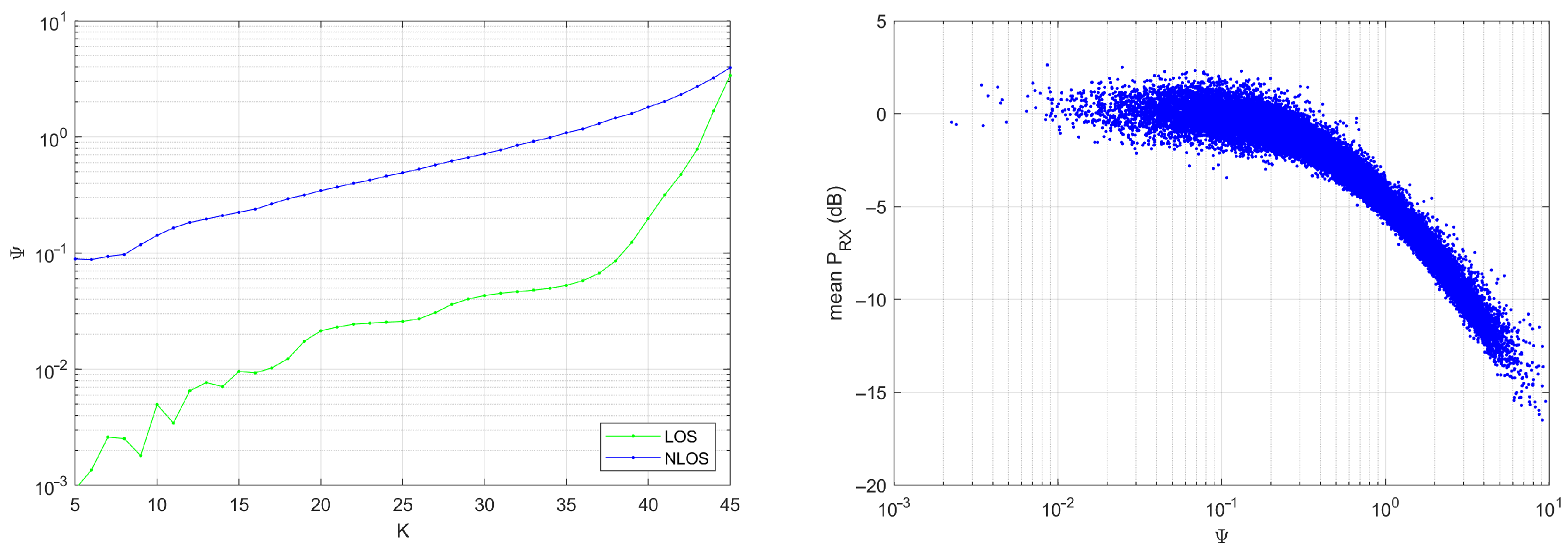
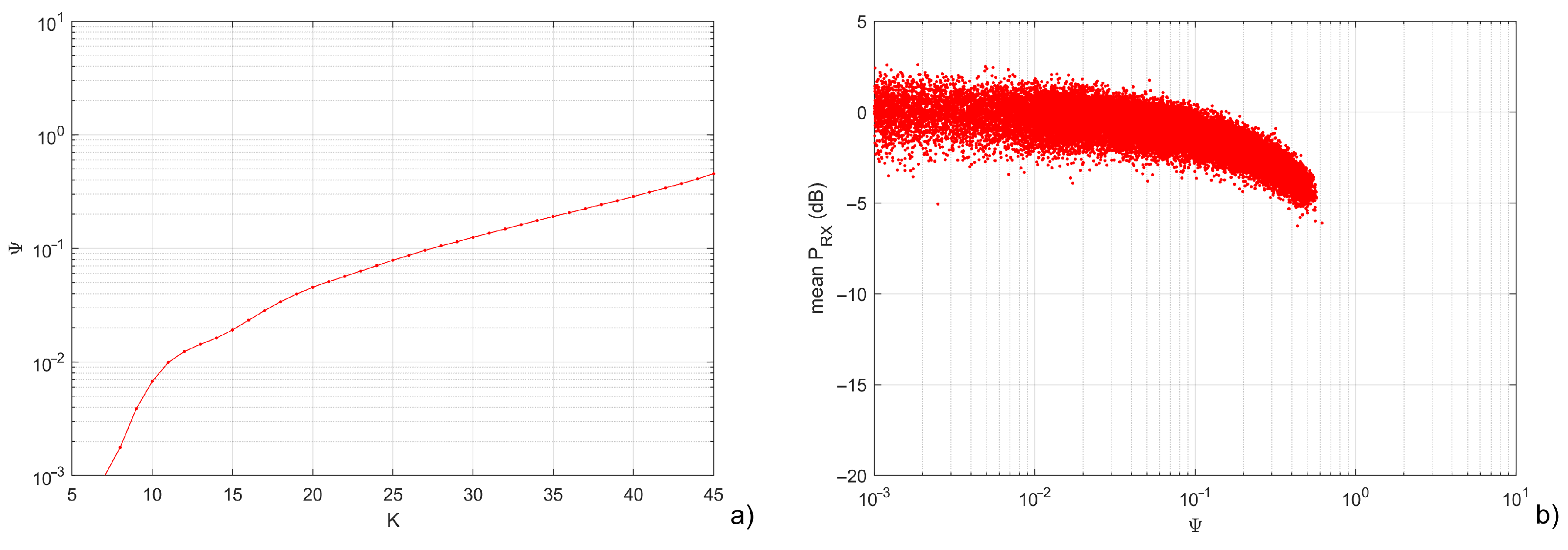
To further investigate these effects, let us now analyze the $\mathsf{\Psi }$ factor of the MU-MIMO channel matrix in the analyzed situation. The $\mathsf{\Psi }$ factor is a channel matrix stability index introduced in [32], and defined as:

$${\mathsf{\Psi }}_{\mathbf{v}}=\frac{\left|\right|{\mathbf{H}}_{\mathbf{v}}{\left|\right|}_F\left|\right|{\mathbf{H}}_{\mathbf{v}}^{†}{\left|\right|}_F}{K}-1$$

(5)

where ${\left|\right|*\left|\right|}_F$ is the Frobenius norm. A $\mathsf{\Psi }$ factor lower than 0.1 is correlated to low beamforming losses (i.e., we have low reduction in the power received by the users due to their being too close from an electromagnetic point of view), while values of $\mathsf{\Psi }$ larger than unity are correlated to infeasible communications, in particular when employing the zero-forcing approach.

In Figure 5a, we can compare the average $\mathsf{\Psi }$ factor for the $P=1000$ different analyzed NLOS scenarios with respect to the LOS scenario. As it is clearly evident, the LOS scenario shows large values of the $\mathsf{\Psi }$ factor only for values of $K\approx M$, while in the NLOS case, it shows significantly larger values. In Figure 5b, we can see a scatter plot correlating the $\mathsf{\Psi }$ factor with the mean received power, showing a strong correlation of values of $\mathsf{\Psi }$ greater than 0.1 with a reduction of the average received power.

The results shown confirm one of the findings currently assumed in the literature that the use of massive MIMO systems with linear processing is convenient for a number of terminals that is approximately one-third of the number of antennas at the BS ($K\approx M/3$).

In a previous work [32], we showed that it was possible to overcome this limitation by properly optimizing the BS antenna. In this paper’s contribution, we will instead show that we can achieve a similar effect by using a controllable local propagation environment around the terminal antennas in such a way that improves the capability of the BS antenna to multiplex the signal toward the users.

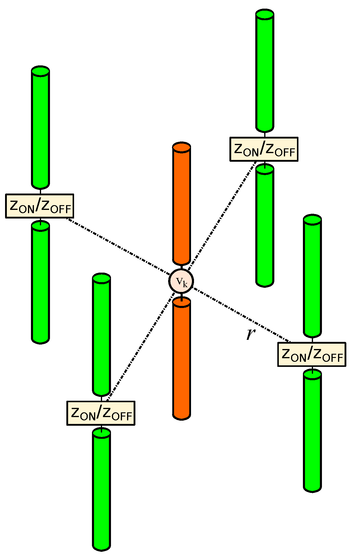
3. A Controllable Local Propagation Environment

Let us consider the antenna architecture depicted in Figure 6, where we realize a controllable local propagation environment around each terminal using parasitic elements that surround the active antenna of the terminal. Each parasitic antenna is connected to a controllable impedance that is able to provide two different values ($Z_{ON},Z_{OFF}$). A system of this kind would be able to provide $P=2^{Np}$ different working states, where $Np$ is the number of parasitic elements employed. It is important to underline a fundamental difference with respect to adding more active antennas to the terminal: the parasitic antennas employed do not require a transceiver to work. It is only required that they are connected to a common controller that provides the required DC signals for controlling the switching of the impedance circuits. In principle, we may consider terminals with several surrounding parasitic elements (prototypes with up to 24 antennas have previously been demonstrated [34]), with a very limited increase in the overall system cost, and we may also employ this technique for the optimization of terminals that have more than one active antenna [46].

3.1. Modelling the CLPE

To model the effect of the parasitic elements, we could use the same approach described in [47]; if we collect in the row vector ${\mathbf{v}}_{OC}$ the open circuit voltages on the $Nt=Np+1$ overall antennas (active+parasitic), induced by the signal radiated by the BS and the non-controllable scattering objects in the scenario, the current signal on the active antenna will be:

$$i_c={\mathbf{V}}_{OC}{\left(\mathbf{Z}+{\mathbf{Z}}_c\right)}^{-1}\mathbf{s}$$

(6)

where $\mathbf{Z}\in \mathcal{C}(Nt,Nt)$ is the impedance matrix describing the coupling between the antennas, ${\mathbf{Z}}_c\in \mathcal{C}(Nt,Nt)$ is a diagonal matrix containing as diagonal elements the receiver’s impedance for the active element and the impedances of the switching circuits for the passive elements, and $\mathbf{s}$ is a column selection vector that selects only the current of the active element (the currents on the parasitic elements are not accessible). It is important to underline that the value of the current $i_c$ depends in a non-linear way on the values of the impedances on the switching circuits used on the parasitic elements.

If we equip each terminal with an antenna using a controllable local propagation environment, the channel matrix will become:

$${\mathbf{H}}_{\mathbf{C}}=\left[\begin{array}{c}{\mathbf{h}}_{1,c_1}\\ {\mathbf{h}}_{2,c_2}\\ ⋮\\ {\mathbf{h}}_{K,c_K}\end{array}\right]$$

(7)

where $\mathbf{C}=[c_1,c_2,\cdots ,c_K]$, with $c_k$ natural numbers in the range $[1,P]$, is a vector defining the configuration of the controllable propagation environment for each one of the K terminals. The values of ${\mathbf{h}}_{k,c_k}$ depend on the geometry of the BS array, the position of the terminal, and the propagation environment where the antennas are communicating. Differently to the case described in the previous section, where the receiving terminals were equipped by a single active element, and the overall MU-MIMO channel matrix was fixed, using the CLPE, we would have the possibility to partially control the overall channel matrix owing to the modification of the local propagation environment.

3.2. Optimizing the CLPE

Some discussion on the optimization of the controllable local propagation environment is now needed.

First, since we have the possibility to control the propagation environment, and hence the realization of the channel matrix, in which way should we change it to achieve the best system performance? The most trivial approach would be the calculation of the power received by each user, the quantity depicted in Figure 3a; however, this approach may not be very practical from a numerical perspective since we would need to recalculate the ZF solution for each terminal, and then calculate the received power using those excitations. Given the result of Figure 5b, we could instead use the $\mathsf{\Psi }$ factor of the channel matrix. It is a good proxy value for the overall MaMIMO performance since it is easy to calculate, and in an optimization procedure, we can simply aim for its minimization: a low $\mathsf{\Psi }$ factor is correlated to good average received powers.

Second, which algorithm could we employ for the minimization of the $\mathsf{\Psi }$ factor? As seen in (6), the relationship between the values of the impedance and the incident field is nonlinear. Moreover, the BS excitation calculated for the $k-$th terminal in (3) is not independent of the excitation used for the remaining $K-1$ terminals: a change in the impedances of the controllable local propagation environment around the $k-$th terminal would influence the response of all the others.

In a communication system employing a reconfigurable local environment using parasitic elements, there would be $P^K$ different possible combinations; this number is too large for an exhaustive search, so we employed an evolutionary algorithm for solving the problem of finding a good combination vector $\mathbf{C}$.

In particular, we implemented a genetic algorithm in which the state of the switches is coded by a gene built as a vector of K real integers (one for each terminal). For the selection, we employ the tournament scheme that considers a number of tournaments equal to the number of terminals K, of three individuals each and uses the calculation of the value of the $\mathsf{\Psi }$ factor of the matrix for the evaluation of individuals. The crossover between the selected elements is realized by generating a random binary mask of K length that mixes the two chosen vectors. For the mutation, we consider a random variation of one of the integer values of the gene. The algorithm employs the overlapping of the generations and the immigration scheme (a new randomly generated individual is added to the population at each iteration) to avoid stagnation of the algorithm around possible local minima. The genetic algorithm is run for a fixed number of 100 iterations, and the computation of an iteration on an Intel i7 8700k processor requires a variable time from 0.1ms to 3ms, depending on the number of terminals $K\in [5,45]$.

This approach is not suitable for “online” operation, but in this paper, we are interested in investigating the maximum possible improvement of the use of a controllable local propagation environment on the multiplexing capability of MaMIMO system. Therefore, the use of a genetic algorithm for the controlling is sufficient for a proof-of-concept. We are currently developing and testing a different controlling algorithm based on deep learning techniques that will be suitable for online operation for rapidly selecting the optimal switch combinations. This algorithm will be the subject of a future paper.

4. Controllable Local Propagation Environment Results

In this section, we will consider a controllable local propagation environment implemented by means of $Np=4$ parasitic antennas, regularly displaced at a distance $r=\lambda /2$; as in the standard case discussed in the previous section, we will use a frequency of $f=3.5$ GHz. For the controllable loads, we will assume that the circuits can switch between two different impedance values, $Z_{ON}=75j\mathsf{\Omega }$ and $Z_{OFF}=-75j\mathsf{\Omega }$; in this case, for each terminal, we have $P=16$ configurations. The parameters describing the structure of the parasitic system ($Np$, r, $Z_{ON}$ and $Z_{OFF}$) were obtained via parametric analysis; in particular, the value of $Np$ was found as a good engineering compromise between the increase in complexity of the antenna and the effectiveness in optimizing the multiplexing capability of the MaMIMO system.

The calculation of the mutual coupling has been performed using the closed form formulas available for wire antenna elements [47], considering a wire length $L=0.48\lambda$ and a wire radius $a=\lambda /2000$.

Once we have evaluated the channel response for each configuration of the switches, we can apply the genetic algorithm for the selection of a good combination vector $\mathbf{C}$. In Figure 7, we can see the patterns of the $K=15$ case for the same propagation channel realization of Figure 2; the patterns of the two cases are slightly different, but we cannot notice qualitative differences between the two.

Let us now look for the same channel realization considered above, at the values of the received channel powers. In Figure 8a, we can see the values of the power level received by the K terminals normalized to the average values when the genetic algorithm has optimized the controllable local propagation environment of the $K=15$ terminals. While the power level for the standard NLOS case showed variations of some dBs between the users, the maximum variations are now limited to no more than 2.5 dB.

The effect seen on this specific channel realization is due to the positive effect of properly selecting the state of the switches of the parasitic elements in the local propagation environment. To better understand the advantage of this reconfigurability, we repeated the same analysis for $P=1000$ different scenarios, the same as those analyzed in the standard NLOS case. We obtained the power level distribution of Figure 8b, in which the power levels, normalized to the average, show an almost Gaussian behavior, with a standard deviation of ${\sigma }_0=0.88$ dB.

As done for the standard LOS case, we repeated the same analysis for a variable number of user terminals. In Figure 9, we can see a representation of the received power level with a range of terminals from 5 to 45. All the powers have been normalized, for the sake of simplicity, to the average power level obtained in the case of $K=5$. The solid red line of the figure represents the average power level received ${\mu }_0$, while the pink area is the area contained between the curves ${\mu }_0-3{\sigma }_0$ and ${\mu }_0+3{\sigma }_0$. The result obtained is much better than the standard case of Figure 4, showing a much smaller spread for all the values of the number of terminals K: the reduction of the minimum power level is not as dramatic as observed in the standard NLOS case, making the communication feasible also with the highest values of K.

For the sake of completeness, we will now analyze the $\mathsf{\Psi }$ factor of the MU-MIMO channel matrix for the controllable local propagation environment case.

In Figure 10a, we show the average $\mathsf{\Psi }$ factor for the $P=1000$ different analyzed controllable local propagation environment case; in particular, the average $\mathsf{\Psi }$ is much lower with respect to the standard NLOS case. In Figure 10b, we can see a scatter plot correlating the $\mathsf{\Psi }$ factor with the mean received power, showing the absence of configurations with $\mathsf{\Psi }$ greater than 1: the maximum reduction of the average received power is in the worst case about 5 dB.

This result provides a very interesting perspective with respect to the results currently assumed in the literature: the use of a controllable local propagation environment allows the use of massive MIMO systems with linear processing with a number of terminals that is close to the number of antennas at the BS ($K\approx M$).

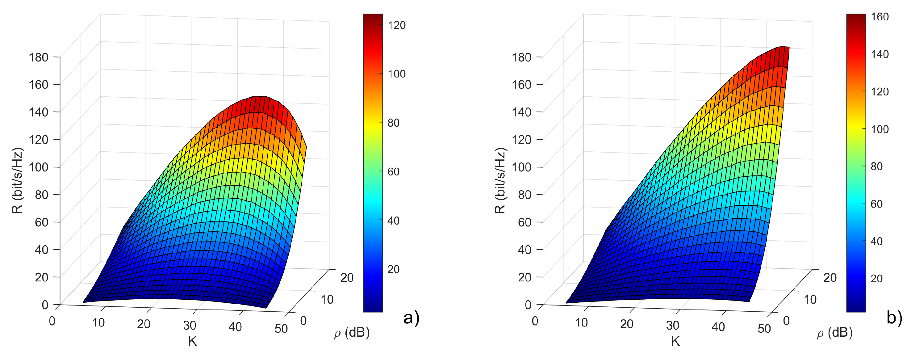
As a final analysis, let us compare the achievable throughput using a controllable local propagation environment. In particular, we will analyze the average transmission rate, evaluated as follows:

$$R=\sum _{k=1}^K{log}_2\left(1+\rho {\xi }_k\right)(bit/s/Hz)$$

(8)

where ${\xi }_k$ is a variable proportional to the square amplitude of the channel attenuation for the $k-$ th user, and $\rho$ is defined as

$$\rho =\frac{P_T{G}_T}{K{\sigma }_n^2}$$

(9)

where $P_T$ is the overall transmitted power, $G_T$ is gain at the transmitting antenna, and ${\sigma }_n^2$ is the variance of the Additive White Gaussian Noise at the user terminal receivers, and the division by K takes into account the fact that the overall transmitted power is equally divided among users, with the same approach of [32].

In Figure 11, we have depicted the average rate achievable by the MaMIMO system when the standard system and the controllable local propagation environment are employed, considering a variation of the number of users and the power-to-noise ratio $\rho$. It is interesting to see that for the lowest number of users, the performances of the two systems are very similar, but when the number of users increases, the controllable local propagation environment case shows a much better transmission rate.

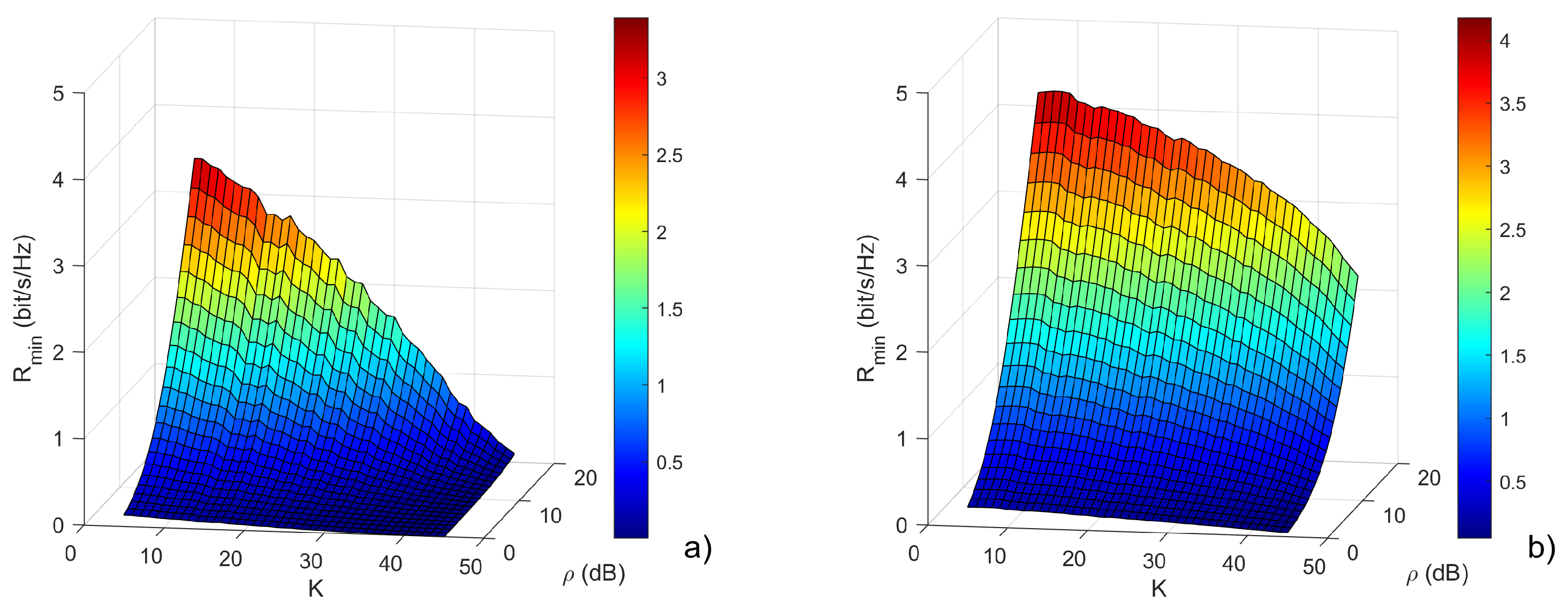
Moreover, to check for channel fairness, we will analyze the minimum rate achieved toward the worst-case user:

$$R_{min}=\underset{k}{min}{log}_2\left(1+\rho {\xi }_k\right)(bit/s/Hz).$$

(10)

In particular, in Figure 12, we calculated the worst-case user rate that is exceeded in 95% of the 1000 simulated scenarios. As evident from the plot, this rate rapidly drops with an increase in the number of users in the standard case. However, its decrease is much less significant when the controllable local propagation environment is used. This means that the controllable local propagation environment promotes channel fairness, making it possible to communicate with more terminals, and guaranteeing a good rate for each one.

5. Conclusions

In this paper, we discuss a novel approach for improving the multiplexing capability of massive MIMO systems. The proposed method employs small parasitic arrays to realize a controllable local propagation environment around user terminals. Differently from RISs, the task of optimizing the propagation channel is shared between the users, and large reconfigurable surfaces are not required to achieve propagation channel optimization.

The proper configuration of user terminals allows a significant increase in the multiplexing capability at the BS that can handle a number of independent channels close to the number of antennas employed at the BS. The numerical simulations performed show a significant improvement with respect to the standard NLOS channel; in particular, the CLPE allows a great enhancement of channel fairness since the use of CLPE guarantees a much smaller spreading of the received power among the different users.

In the considered calculations, we did not employ scheduling approaches, so it may be possible to achieve further improvements if smart scheduling approaches are used together with the controllable local propagation environment. It is also worth noting that in the example shown, all the antenna terminals used a CLPE. Still, it may also be possible to exploit it only for some terminals, such as those that are in more crowded regions of space, simplifying the implementation of the overall communication system.

Regarding future study, we are working towards analyzing the effect of a controllable local propagation environment in indoor MaMIMO systems, in addition to a measurement campaign that will provide experimental verification of the simulation results. Finally, we are also investigating the use of deep learning techniques to accelerate the controllable local propagation environment configuration procedure, making it possible to perform an “online” operation using these kinds of systems.