Connectivity Analysis with Co-Channel Interference for Urban Vehicular Ad Hoc Networks

Abstract

In urban vehicular ad hoc networks (VANETs), the complex channel environment and co-channel interference resulted in the uncertain delay of inter-vehicle packet transmission, which causes serious delay jitter. Connectivity is proposed as a key metric to describe this uncertainty. However, existing works lack a discussion of inter-vehicle connectivity in urban VANETs, particularly with regards to the process of transmitting packets between vehicles. In this paper, we analyze the connectivity probability of urban VANETs under co-channel interference with both complete and incomplete information. When the information is complete, we model the time-varying nature of co-channel interference and channel fading as delay jitter and analyze inter-vehicle connectivity in a time-varying environment. Then, when complete information is unavailable, we estimate the probability distribution of co-channel interference by combining the distribution of multiple parameters with the free space propagation model (Friss) model and Nakagami-m fading model. The expression for the connectivity performance of vehicle-to-vehicle (V2V) links is derived from the signal interference plus noise ratio (SINR) of the destination V2V link. Finally, we analyze the implications of various factors on connectivity, such as the transmit power of the signal, the arrival rate of packets, the number of channels and vehicles, and the distance between the transmitting vehicle and the receiving vehicle. The numerical analysis shows that co-channel interference and signal fading significantly affect inter-vehicle connectivity.

1. Introduction

As an important component of intelligent transport systems (ITS) [1], vehicular ad hoc networks (VANETs) have received extensive attention from academia and industry [2,3,4]. Vehicle-to-vehicle (V2V) communication has been developed as a key technology in enhancing transportation and road safety by supporting cooperation among vehicles in close proximity. Due to the safety imperative, the quality-of-service (QoS) requirements for V2V communication are very stringent with ultra-low latency and high-reliability [5], especially in 5G [6,7]. VANETs also enable collaborative safe vehicle driving; intelligent regional traffic dispatch; intersection decision support; real-time traffic information distribution; and applications in interactive streaming communications such as P2P file sharing, video transmission, and online gaming. The creation of these applications has made it necessary for VANETs to deal not only with the transmission of separated packets but also with the transmission of continuous packets.

However, in urban block scenarios, channel fading and co-channel interference are severe, and the topology and node density of VANETs constantly change. This leads to problems such as packet loss, retransmissions and collisions, or even the interruption of communication in severe cases [8]. As a corollary, end-to-end communication cannot be guaranteed in VANETs. This indeterminacy greatly raises the risk of urban transport. In order to describe this instability, connectivity has been proposed as a key metric to describe the communication status between vehicles.

1.1. Motivation

Inter-vehicle connectivity plays a critical role in VANETs. However, urban VANETs face various issues and challenges, such as co-channel interference, which significantly affects VANETs connectivity. To effectively address these challenges, it is essential to gain a deeper understanding of the impact of co-channel interference on inter-vehicle connectivity. Therefore, this paper aims to analyze the impact of co-channel interference on connectivity using both complete and incomplete channel information. Specifically, we model the temporal variability of co-channel interference as delay jitter and examine its effect on VANETs connectivity. Additionally, we analyze the connectivity of VANETs with incomplete co-channel interference information when complete information is unavailable. By utilizing various parameters and estimation methods related to co-channel interference, along with the free space propagation model (Friss) model and the Nakagami-m fading model, we can gain a better understanding of the impact of co-channel interference on VANETs and provide valuable insights for achieving efficient inter-vehicle connectivity.

1.2. Contributions

The main contributions of this paper are summarized as follows.

• We analyze the impact of time-varying co-channel interference on connectivity in VANETs with complete information availability. Assuming that the co-channel interference distribution satisfies an independent identical distribution, the time-varying nature of co-channel interference is modeled as delay jitter to obtain the connectivity probability of inter-vehicle packets in urban VANETs.
• We conduct an analysis on how uncertain co-channel interference affects the connectivity of V2V communication links, where complete information is not available. The distribution of co-channel interference is estimated using several parameters related to co-channel interference, such as vehicle position, transmission power, and fading coefficient, in combination with the Friss model and Nakagami-m fading model. The CLT is also used to estimate the distribution of the total co-channel interference. The inter-vehicle connection probability is obtained from the SINR of the destination signal.
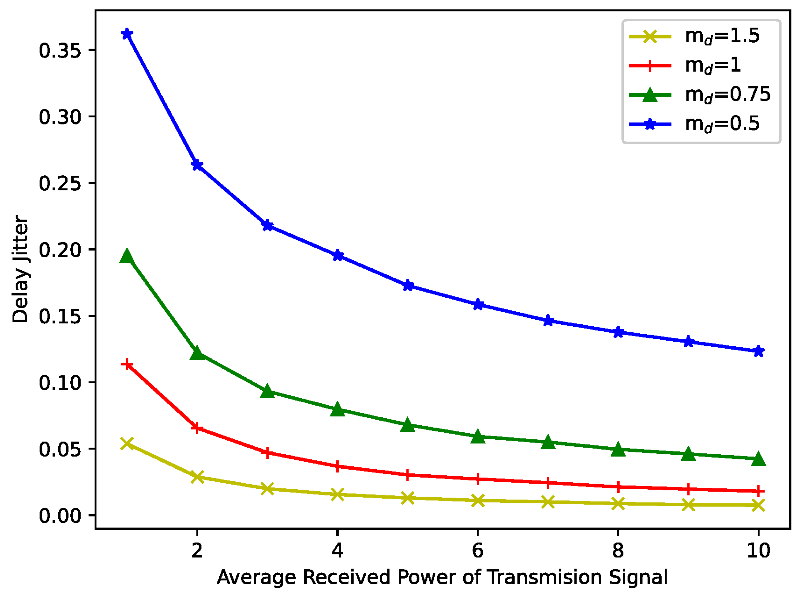
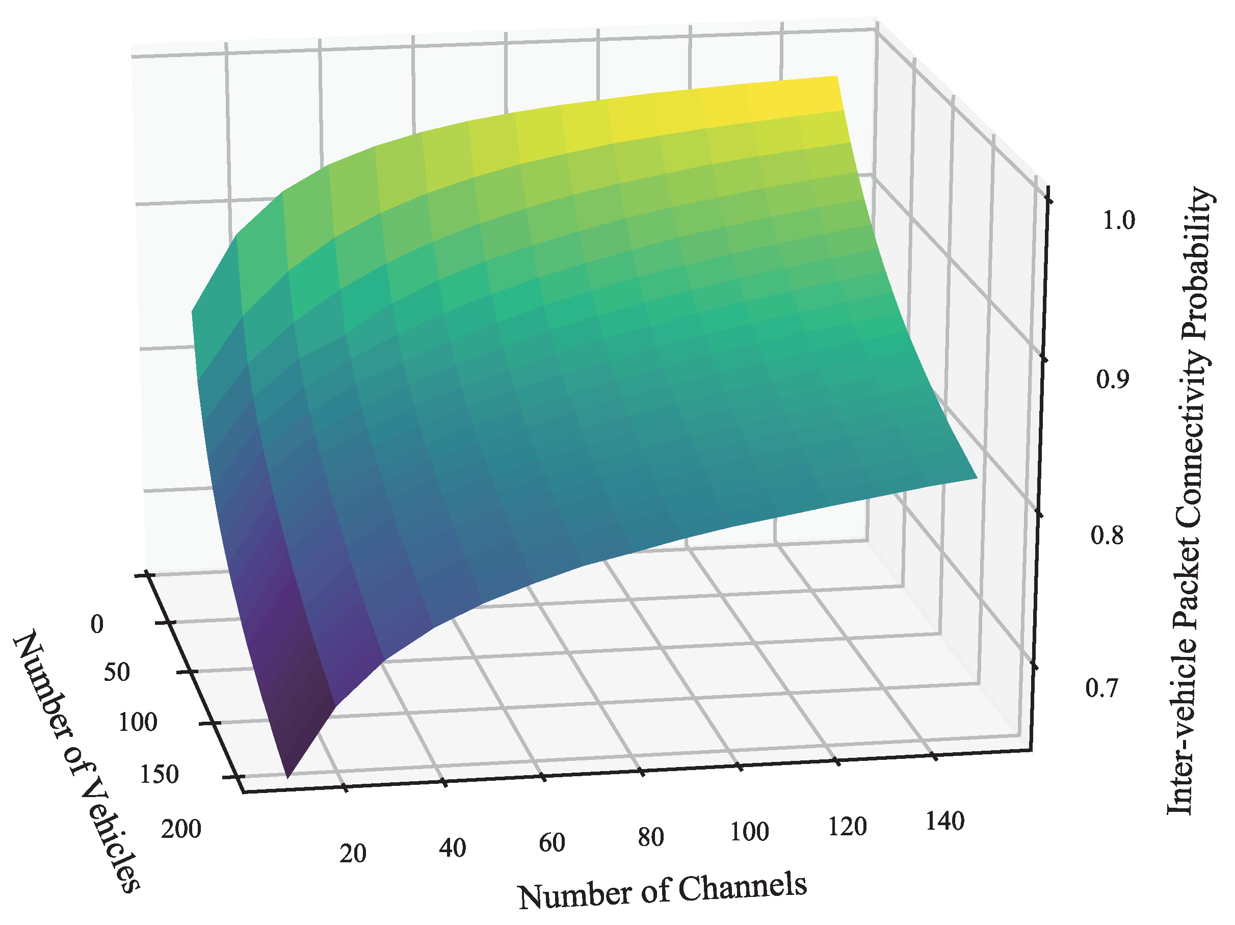
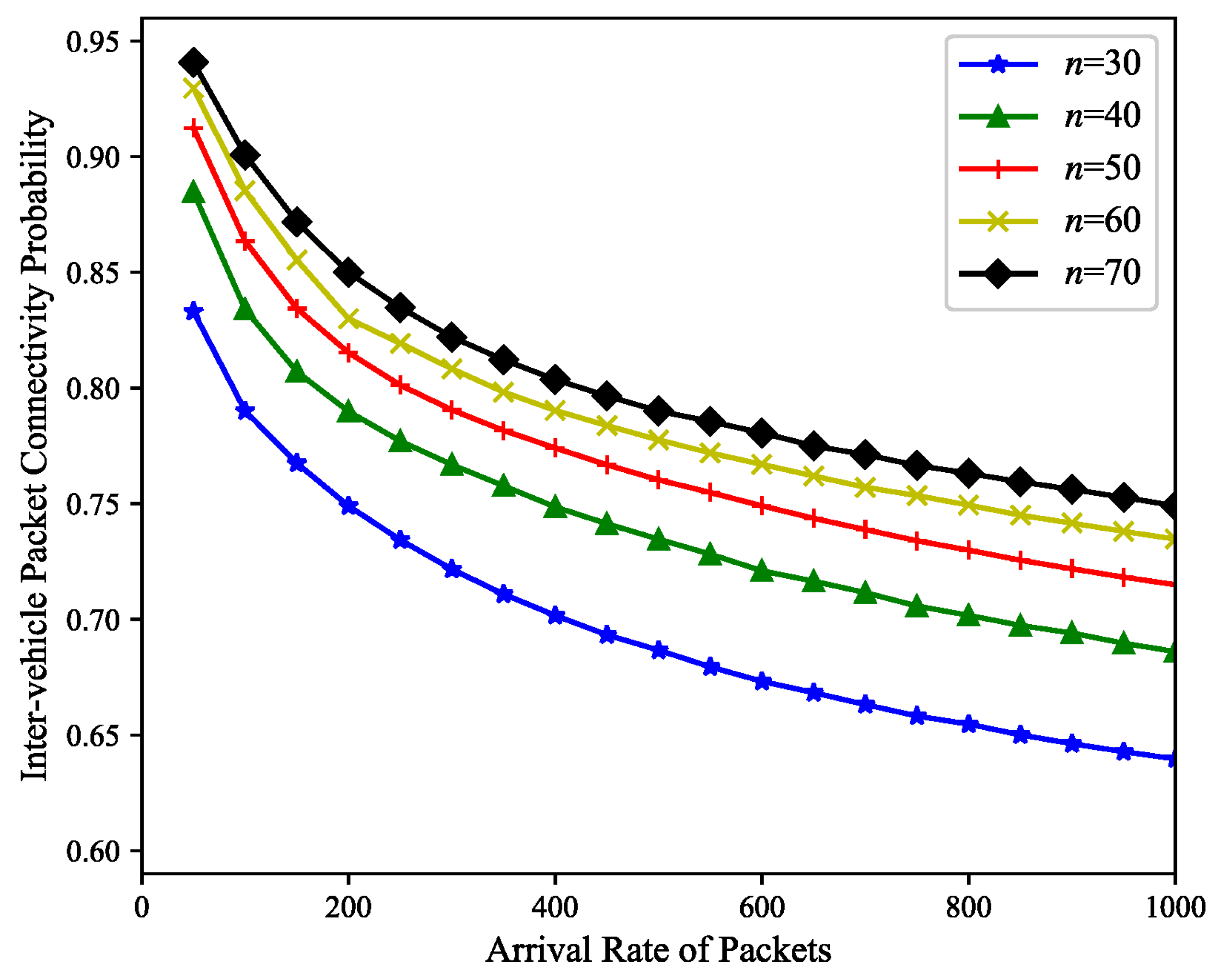
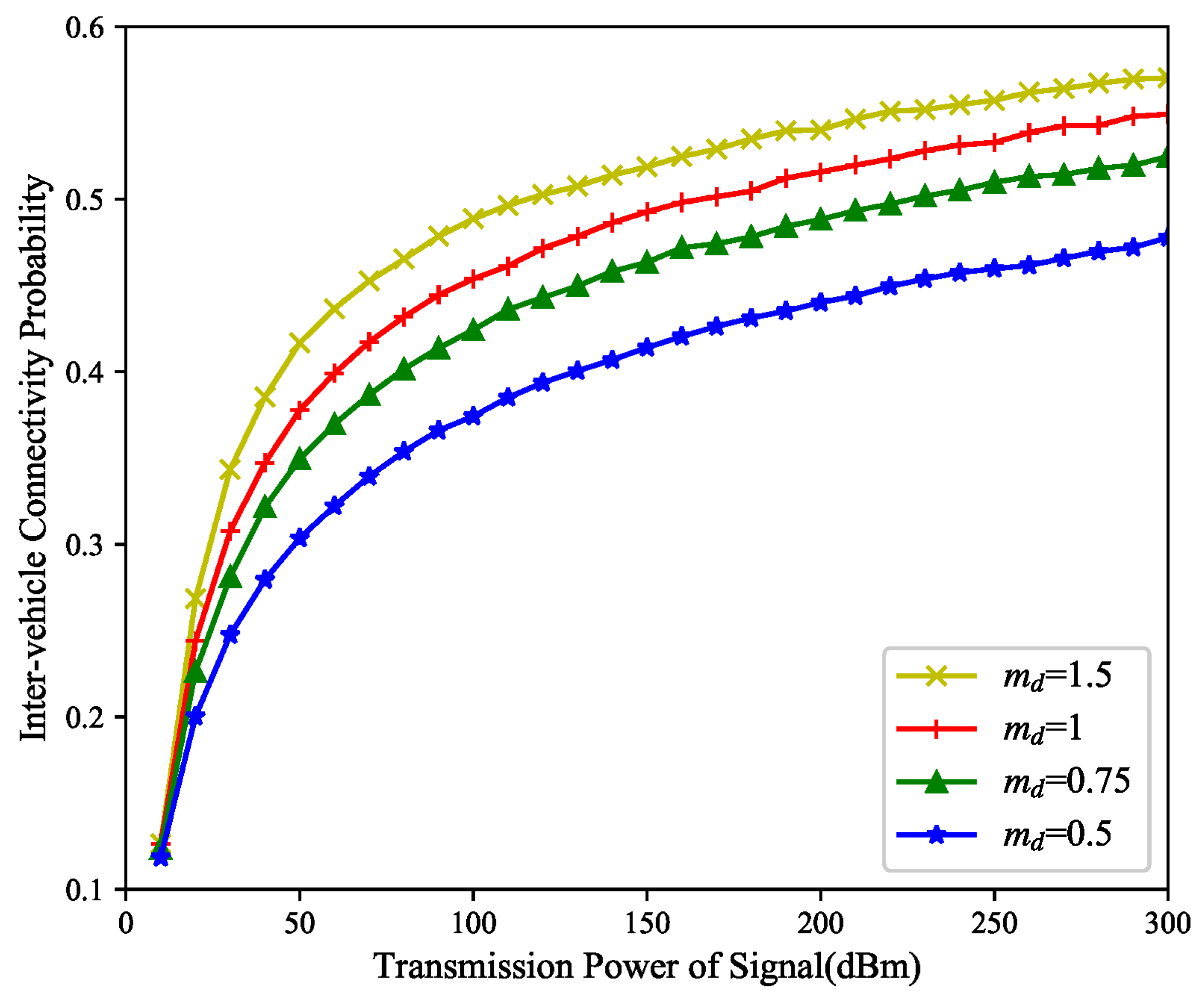
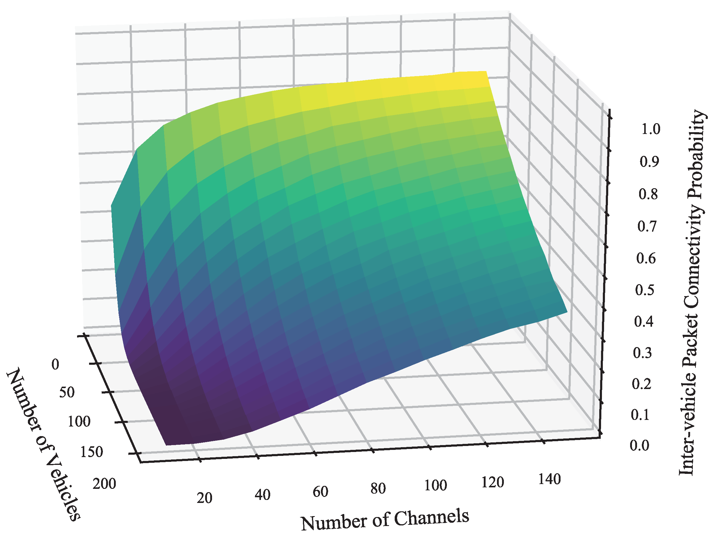
• We numerically analyze the impact of several key parameters such as the number of surrounding vehicles, the arrival rate of packets, and the fading factor, on inter-vehicle packet connectivity and inter-vehicle V2V link connectivity. We find that the effects of co-channel interference are non-negligible, both for inter-vehicle V2V links and for packet transmission. Packet transmission is more sensitive to co-channel interference when packet arrival rates increase and the fading of the channel becomes severe.

1.3. Paper Outline

The remainder of this paper is structured as follows. Section 3 presents the system model. Section 4 analyzes the connectivity of VANETs with complete channel information. Section 5 analyzes the connectivity of VANETs with incomplete channel information. Section 6 simulates the effect of each parameter on the connectivity. Finally, Section 7 presents the conclusions of the paper.

2. Related Work

Numerous scholars have worked to accurately describe the connectivity between vehicles. It is commonly accepted that inter-vehicle connectivity is impacted by the influence of traffic flow rate, interference, and signal fading [9,10]. The probability of vehicles communicating successfully with each other is calculated using information such as the location of the vehicles and the power of the signals, also known as the probability of connectivity. Typically, vehicles are considered to be independent of each other and free-flowing on the road, and their arrival follows a Poisson process. In the literature, numerous V2V connectivity studies [11,12,13,14,15] have relied on this assumption. Moreover, other theoretical and empirical models have been attempted for more accurate traffic modeling in other traffic conditions [16,17].

Interference and channel fading have a significant impact on connectivity, which are essential components in the analysis of connectivity. How the communication channel is modeled impacts the accuracy of inter-vehicle connectivity analysis greatly. Some current studies relied on the unit-disk model as the signal propagation model [11,12,18,19], which is a fixed communication range model. If the distance between vehicles is less than the communication range of vehicles, then the two vehicles are denoted as connected. The probability of inter-vehicle connectivity is expressed as the probability that the receiving vehicle is within the communication range of the transmitting vehicle. For example, B. Pan et al. analyzed the impact of user behavior, namely, the willingness of users to act as relays to assist others in forwarding messages and other system parameters on the probability of connectivity in [12]. Additionally, the conclusion that user behavior cannot be ignored is drawn. In [15], C. Bian et al. analyzed the probability of vehicles or platoons being connected to the infrastructure either directly or via a relay on a two-way lane. The communication model of the vehicle is modeled as a unit-disk model. Three different communication ranges are defined to distinguish between BSs, platoons, and normal vehicles. In [20], J. Zhao et al. studied the probability of vehicle-to-infrastructure (V2I) connectivity in a multi-hop network, whereas the unit-disk model defines the propagation of the signal in an over-ideal and simplistic way, ignoring the fading and co-channel interference that can occur between vehicles in VANETs. In urban block scenarios, the buildings, trees, and so on can cause the reflection and refraction of the signal, resulting in severe channel fading, where there may be instances of co-channel interference between vehicles. Therefore, the unit-disk model is not suitable for connectivity analysis in urban VANETs [21,22].

Attempts have been made to analyze inter-vehicle connectivity using models that are closer to actual fading. The most common models are the Rayleigh, Ricean, and Nakagami-m fading models. The Rayleigh fading model is used to represent channel randomness in the absence of line-of-sight signals, while Ricean is used in the presence of direct signals between two nodes. However, the Nakagami-m fading model is considered more suitable for describing randomness channels because it can flexibly reflect the diversity of VANETs scenarios, such as urban, highway, and rural areas, and it is more in proximity to the severe fading in VANETs [22]. In [23], S.M. Hanshi et al. utilized the Nakagami-m fading model to describe the distribution of the received signal strength, verifying that the Nakagami-m model can represent a wide range of channel randomness scenarios. However, channel resources are limited, and co-channel interference may occur between vehicles using the same channel. Not only signal fading but also co-channel interference needs to be taken into account. In [24], R. Chen et al. evaluated the effect of user behavior on connectivity probability in a highway scenario. User behavior is defined as a willingness to act as a relay node for forwarding messages. The Nakagami distribution was modeled for the user’s transmitted and interfering signals, and a closed-form expression for inter-vehicle connectivity probability was obtained for both a deterministic and an uncertain number of interference signals.

However, there are more than just the above issues to consider when it comes to continuous packet transmission. In a fast time-varying scenario such as urban VANETs, the rapid movement of vehicles and channel fading can lead to rapid changes in the SINR of the received signal, resulting in variations of packet-transmission delay, known as delay jitter. The phenomenon of excessive delay and jitter in V2V communication can significantly impact connectivity, leading to packet loss and retransmission, ultimately compromising quality and stability [25,26,27,28,29,30]. Although these works analyze the connectivity performance under fading channels and consider co-channel interference between vehicles, they cannot handle the challenges posed by the time-varying environment. Therefore, it becomes crucial to analyze inter-vehicle connectivity under different environmental conditions, ensuring effective maintenance of VANETs.

In summary, analyzing inter-vehicle connectivity in VANETs is a complex and multifaceted problem that demands a thorough understanding of various factors such as traffic flow rate, interference, signal fading, and channel models. Extensive research has been conducted using various theoretical and empirical models to simulate and analyze these factors accurately. Although some models, such as the unit-disk model, provide a simple and effective way to analyze connectivity, they fail to consider the impact of attenuation and interference, which is crucial in urban VANETs. The Nakagami-m fading model provides greater realism by accounting for these factors. Additionally, the time-varying nature of VANETs and the impracticality of vehicles obtaining real-time global information presents significant challenges for inter-vehicle connectivity analysis. Therefore, further research is necessary to address these challenges.

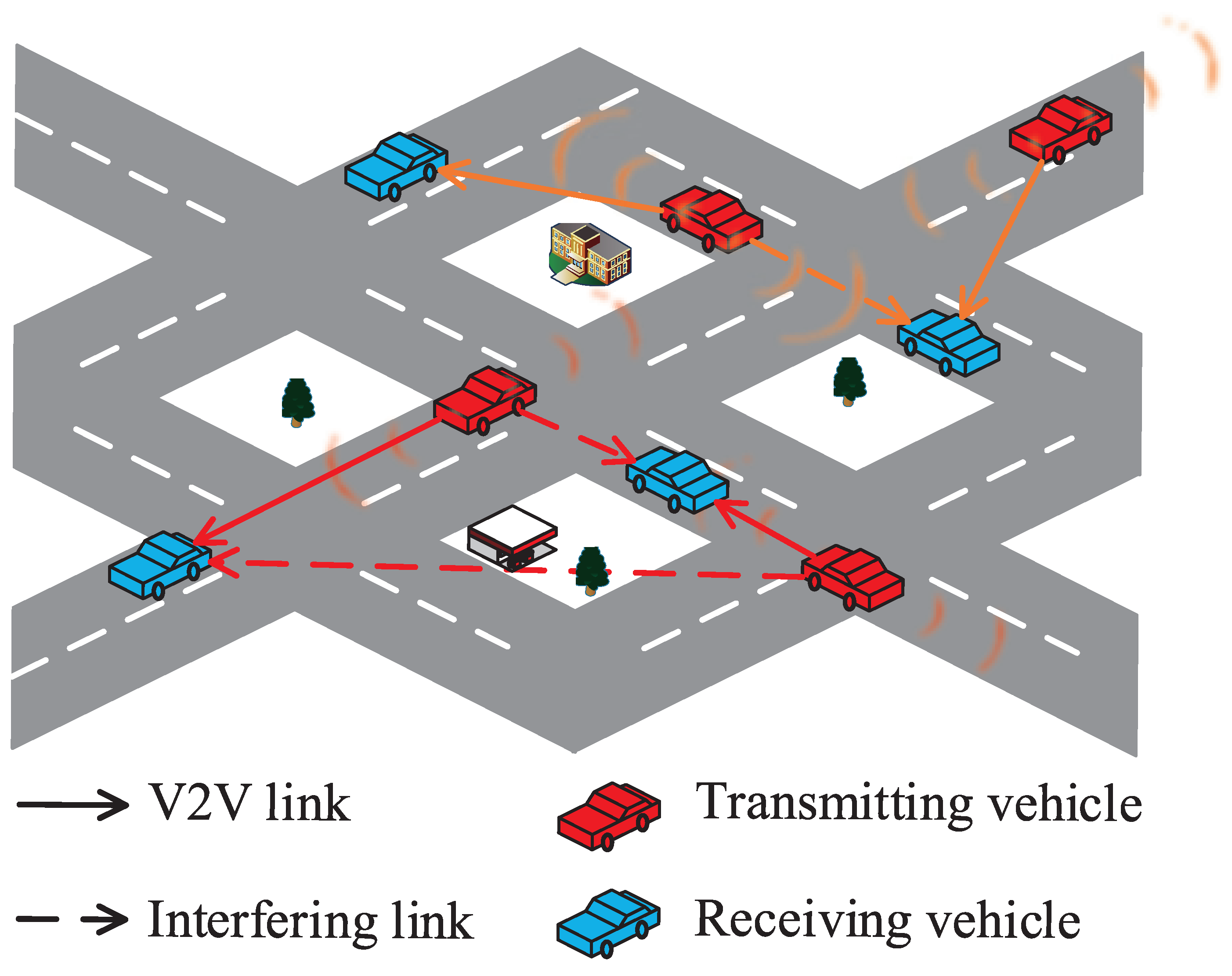
3. System Model

We consider the VANETs in the urban VANETs as depicted in Figure 1. In this model, vehicles are deployed on the road according to a certain model with a total number of U. Each vehicle is equipped with a single antenna. On the one hand, each vehicle can relay messages sent or received; on the other hand, the vehicles are equipped with a V2V interface to communicate with each other. We assume that there are K limited channels available for communication and that vehicles choose their channels in a completely random way. Therefore, co-channel interference between vehicles may occur with a probability of $1/K$. Although there is a temporal correlation between these factors, including the mobility of vehicles, time-varying fading of signals during transmission, and the number of surrounding vehicles, they change relatively slowly. Therefore, this article does not consider their temporal nature. Nevertheless, due to the fluctuating occupation of channels by surrounding vehicles in each time slot, the interference on the same channel exhibits some level of temporal correlation. This leads to a delay jitter phenomenon in the packets.

3.1. Traffic Flow Model

In traffic theory, the movement of vehicles is independent. Without a loss of generality, we assume that vehicles enter the road in a Poisson process with a flow rate of $\rho$. Then, the probability that there are n vehicles on a road of length x can be expressed as

$$f(n,x)=\frac{{\left(\rho x\right)}^n{e}^{-\rho x}}{n!},n\ge 0.$$

(1)

Given that the number of vehicles in a certain section is n, the vehicles are uniformly distributed over the location, according to the demonstration in the literature [31]. Set the length of the road as $L_d$ and the shortest distance between vehicles as the safe distance $L_s$. The probability of the distance between the receiving vehicle and the transmitting vehicle can be expressed as

$$f_D\left(d\right)=\frac{1}{L_d-L_s}.$$

(2)

3.2. Radio Propagation Model

In urban VANETs, the signal is heavily attenuated due to shading by trees and buildings and the mobility of vehicles. For a realistic fit, we denote the envelope of the received dominant signal as R and assume that the envelope meets the Nakagami distribution. The PDF of the received signal envelope can be expressed as

$$f_R\left(r\right|m,{\overline{p}}_r)=\frac{2}{\mathsf{\Gamma }\left(m\right)}{\left(\frac{m}{{\overline{p}}_r}\right)}^m{r}^{2m-1}{e}^{-\frac{m}{{\overline{p}}_r}{r}^2},$$

(3)

where ${\overline{p}}_r=E\left(R^2\right)$, with $E(·)$ being the expectation of a random variable; m is the the Nakagami fading factor, which represents the loss of the signal during transmission [32]; and $m\ge 0.5$, $\mathsf{\Gamma }\left(m\right)={\int }_0^{\infty }{x}^{m-1}{e}^{-x}dx$ is the Gamma function. The severity of fading on wireless channels is measured in terms of m, with severe fading occurring when m is small and weak fading occurring when m is large [33].

The received power $P_r$ can be represented by $P_r=R^2$. According to the PDF of R, the random variable $P_r$ follows a Gamma distribution as $G(m,{\overline{p}}_r)$, and the PDF can be written as

$$f_{P_r}\left(p_r\right|m,{\overline{p}}_r)=\frac{1}{\mathsf{\Gamma }\left(m\right)}{\left(\frac{m}{{\overline{p}}_r}\right)}^m{p_r}^{m-1}{e}^{-\frac{m}{{\overline{p}}_r}{p}_r}.$$

(4)

Since the interference is randomly generated by surrounding vehicles, we define the set ${\left\{P_{c,i}\right\}}_{i=0}^n$ as the set of n independent distributed interference powers. Consequently, the total co-channel interference power $P_c$ can be expressed as

$$P_c=\sum _{i=1}^n{P}_{c,i}.$$

(5)

The effect of the ith interfence signal can be represented as $P_{c,i}\sim G(m_{c,i},{\overline{p}}_{c,i})$. The random variable $SINR$ is defined to represent the SINR of the received signal; it can be expressed as

$$SINR=\frac{P_r}{N_0+P_c}=\frac{P_r}{N_0+\sum _{i=1}^n{P}_{c,i}},$$

(6)

where $N_0$ is the power of the additive white Gaussian noise (AWGN).

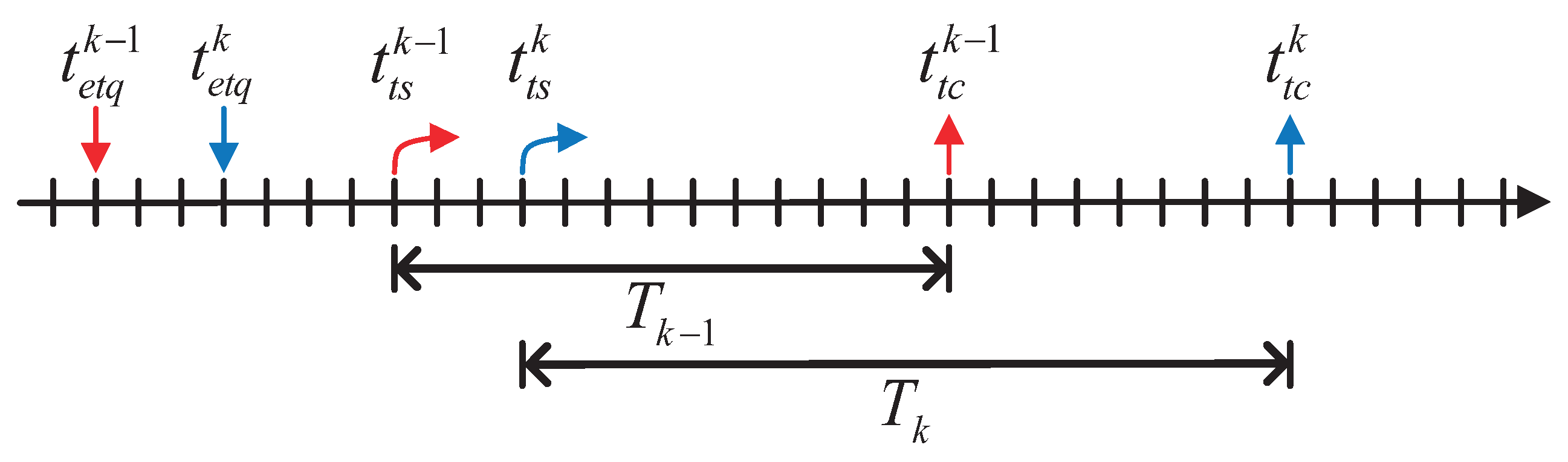
3.3. Delay Jitter Model

Delay jitter is mapped as the change in packet-transmission delay, depending on the packet transmission process. In this paper, we use the definition of delay jitter from the IETF [34]. It is based on the transmission time and delay between the packet transmission’s beginning and end. As shown in Figure 2, the $(k-1)$th packet and the kth packet enter the transmission queue at time slot $t_{etq}^{k-1}$ and $t_{etq}^k$. The time interval between $t_{etq}^{k-1}$ and $t_{etq}^k$ is $\tau$ time slots. Then, the $(k-1)$th packet and the kth packet starts transmission at time slot $t_{ts}^{k-1}$ and $t_{ts}^k$ after the same waiting time $t_w$, arriving at the receiving vehicle at time slots $t_{tc}^{k-1}$ and $t_{tc}^k$, respectively. The transmission times are $T_{k-1}$ and $T_k$, respectively.

According to Shannon’s formula, the delay $T_k$ experienced during the transmission of the kth packet can be expressed as

$$T_k=\frac{size}{w{log}_2(1+SIN{R}_k)}=\frac{sizeln2}{wln(1+SIN{R}_k)},$$

(7)

where $size$ is the size of the packets and w is the bandwidth of the channels. We assume that both the packets’ size and the bandwidth of the channels are constant. Since the Taylor series expansion of $ln(1+SINR)$ in the range $(0,\infty )$ is

$$ln(1+SINR)=2\sum _{k=0}^{\infty }\frac{1}{2k+1}\frac{1}{{(SINR+2)}^{2k+1}},$$

(8)

we approximate $ln(1+SINR)$ as $\frac{2}{SINR+2}$. Then, the delay jitter, which is the difference in transmission time between two consecutive packets, can be expressed as

$$J_k=T_{k-1}-T_k=\frac{sizeln2}{2w}(SIN{R}_{k-1}-SIN{R}_k).$$

(9)

When the delay jitter is dramatic, packets become disordered at the receiving vehicle and may be lost. Therefore, we assume that the packet transmitted between vehicles is connected when the $(k-1)$th packet is received before the kth packet; otherwise, it is not connected. The connectivity probability of packets is defined as the successful transmission probability of packets. It represents the probability that the time interval $\eta$ between two consecutive packets entering the transmission queue is greater than the $(k-1)$th packet transmission time minus the kth packet transmission time, denoted as

$$P_{CoJ}=Pr\{\eta >J_k\}=Pr\{\eta >T_{k-1}-T_k\}.$$

(10)

4. Probabilistic Analysis of Connectivity in VANETs with Complete Information

In this section, we analyze the connectivity performance of VANETs with complete information. The time-varying nature of co-channel interference is described as delay jitter. We utilize the inter-vehicle packet connectivity probability to reflect the connectivity probability of VANETs. When packets are sent from transmitting vehicles to receiving vehicles, the transmission delay of packets jitters due to the effects of the co-channel interference and the unstable channel state of the V2V links. The packets will be disordered when they are received at the receiving vehicle. To derive an expression for the probability of inter-vehicle packet connectivity, we assume that co-channel interference is independent and identically distributed. We first analyze the PDF of the time consumed to transmit data of size $size$. Then, the probability that the delay jitter is lower than the interval between packets entering the transmission queue is analyzed according to the definition of delay jitter.

4.1. PDF of the Destination V2V Link’s SINR

We assume that the distance and the communication environment of V2V links between the interfering vehicle and receiving vehicle are approximately the same. Hence, all of the interferences have identical distribution statistics. If the number of interfering vehicles is given, and in accordance with the additivity of the Gamma distribution, we can obtain the PDF of the total co-channel interference power $P_{c,v}$ generated by v vehicles as

$$\begin{array}{cc}\hfill & f_{P_{c,v}}\left(p_{c,v}\right|vm,{\overline{p}}_c)=\frac{1}{\mathsf{\Gamma }\left(v{m}_c\right)}{\left(\frac{m_c}{{\overline{p}}_c}\right)}^{v{m}_c}{p_{c,v}}^{v{m}_c-1}{e}^{-\frac{m_c}{{\overline{p}}_c}{p}_{c,v}},\hfill \end{array}$$

(11)

where ${\overline{p}}_c$ is the average interference power of each interfering signal, and $m_c$ is the Nakagami fading factor of interfering vehicles. In the actual scenario, the surrounding vehicles select the transmission channel randomly, and each vehicle may interfere with the link. We establish whether a vehicle is an interfering vehicle and meets the binomial distribution; the probability of that is $1/K$. Then, the probability of V vehicles reusing the link’s channel can be expressed as

$$Pr\{V=v\}=\left(\begin{array}{c}n\\ v\end{array}\right){\left(\frac{1}{K}\right)}^v{(1-\frac{1}{K})}^{n-v},$$

(12)

where $\left(\begin{array}{c}n\\ v\end{array}\right)$ is the combinatorial number, indicating the number of all combinations of $m(m\le n)$ elements from n different elements.

According to the power of AWGN, which is fixed, and (6), (11), and (12), the PDF of total interfering power $P_I$ can be written as

$$\begin{array}{cc}\hfill f_{P_I}\left(p_I\right)=& \sum _{v=0}^n\left(\begin{array}{c}n\\ v\end{array}\right){\left(\frac{1}{K}\right)}^v{(1-\frac{1}{K})}^{n-v}\frac{1}{\mathsf{\Gamma }\left(v{m}_c\right)}{\left(\frac{m_c}{{\overline{p}}_c}\right)}^{v{m}_c}{(p_I-N_0)}^{v{m}_c-1}{e}^{-\frac{m_c}{{\overline{p}}_c}(p_I-N_0)}.\hfill \end{array}$$

(13)

For the destination V2V links, we assume that the mean value ${\overline{p}}_d$ and Nakagami fading factor $m_d$ of the received signal are both known and that the received signals follow the Gamma distribution as $G(m_d,{\overline{p}}_d)$. Then, the PDF of received signals’ SINR can be obtained from (4), (6), and (13) and represented as

$$f_{SINR}\left(sinr\right)={\int }_0^{\infty }{p}_I{f}_{P_d}\left(p_{I}sinr\right)f_{P_I}\left(p_I\right)d{p}_I.$$

(14)

The ${(p_I-N_0)}^{v{m}_c-1}$ in (13) is expressed in terms of a Newtonian binomial expansion as

$$\begin{array}{cc}\hfill {(p_I-N_0)}^{v{m}_c-1}=& \sum _{k_1}^{\infty }\left(\begin{array}{c}v{m}_c-1\\ k_1\end{array}\right){(-N_0)}^{v{m}_c-1-k_1}{p_I}^{k_1},\hfill \end{array}$$

(15)

where $\left(\begin{array}{c}m\\ n\end{array}\right)=\frac{m(m-1)\cdots (m-n+1)}{n!}$ is a combinatorial number in the form. According to (3.478.1) in [35], (14), and (15), the PDF of $SINR$ can be further obtained as

$$\begin{array}{cc}\hfill f_{SINR}\left(sinr\right)=& \sum _{v=0}^n\sum _{k_1}^{\infty }f(v,k_1)sin{r}^{m_d-1}{(\frac{m_c}{{\overline{p}}_c}+\frac{m_d}{{\overline{p}}_d}sinr)}^{-(m_d+k_1)},\hfill \end{array}$$

(16)

where $f(v,k_1)$ is a coefficient independent of $SINR$, can be expressed as

$$\begin{array}{cc}\hfill f(v,k_1)=& \left(\begin{array}{c}n\\ v\end{array}\right){\left(\frac{1}{K}\right)}^v{(1-\frac{1}{K})}^{n-v}\frac{\mathsf{\Gamma }(m_d+k_1)}{\mathsf{\Gamma }\left(v{m}_c\right)\mathsf{\Gamma }\left(m_d\right)}{\left(\frac{m_c}{{\overline{p}}_c}\right)}^{v{m}_c}{\left(\frac{m_d}{{\overline{p}}_d}\right)}^{m_d}\hfill \\ & exp\left(\frac{m_c{N}_0}{{\overline{p}}_c}\right)\left(\begin{array}{c}v{m}_c-1\\ k_1\end{array}\right){(-N_0)}^{v{m}_c-1-k_1}.\hfill \end{array}$$

(17)

4.2. VANETS Connectivity Probability in View of Delay Jitter

In general, we assume that there is no correlation between the data transmitted between vehicles, and the generation of packets meets a Poisson distribution

$$f(n_p,\tau )=\frac{{\left(\lambda \tau \right)}^{n_p}{e}^{-\lambda \tau }}{n_p!},n_p\ge 0,$$

(18)

where $\lambda$ is the arrival rate of packets, i.e., the number of packets entering the transmission queue per second, $n_p$ is the number of packets, and $\tau$ is the duration. In addition, the probability that there are no packets in an interval $\tau$, which is the probability that the packet generation interval $\eta$ is greater than $\tau$, is given by

$$Pr\{\eta >\tau \}=f(0,\tau )=e^{-\lambda \tau }.$$

(19)

So, the inter-vehicle connectivity probability can be represented by

$$P_{CoJ}=e^{-\lambda \tau }.$$

(20)

Define $\mathsf{\Theta }=SIN{R}_{k-1}-SIN{R}_k$ as the difference between two consecutive packet $SINR$. According to (16), and after several Newtonian generalized binomial expansions, the PDF of $\mathsf{\Theta }$ can be represented as

$$\begin{array}{cc}\hfill f_{\mathsf{\Theta }}\left(\theta \right)=& {\int }_0^{\infty }{f}_{SINR}(sin{r}_k+\theta )f_{SINR}\left(sin{r}_k\right)dsin{r}_k\hfill \\ \hfill =& \sum _{v=0}^n\sum _{k_1=0}^{\infty }\sum _{v^{\prime }=0}^n\sum _{{k^{\prime }}_1=0}^{\infty }f(v,k_1)f(v^{\prime },k_1^{\prime })\sum _{k_2=0}^{\infty }\left(\begin{array}{c}{m}_d+k_1+k_2-1\\ k_2\end{array}\right)\hfill \\ \hfill & \sum _{k_3=0}^{\infty }\left(\begin{array}{c}{m}_d-1\\ k_3\end{array}\right)\sum _{k_4=0}^{\infty }\left(\begin{array}{c}{m}_d-1+k_3\\ k_4\end{array}\right){(-1)}^{m_d-1+k_2+k_3-k_4}\hfill \\ \hfill & {\left(\frac{m_d}{{\overline{p}}_d}\right)}^{m_d+k_1-k_2-k_3}{\left(\frac{m_c}{{\overline{p}}_c}\right)}^{k_2+k_3-k_1}\frac{{\theta }^{2m_d-1+k_1-k_2-k_3}}{(k_2+k_4-m_d-k_1+1)}.\hfill \end{array}$$

(21)

The delay jitter J between two consecutive packets can be calculated from $\mathsf{\Theta }$, and the PDF of delay jitter J can be calculated as

$$\begin{array}{c}\hfill f_J\left(j\right)=\frac{2w}{sizeln2}{f}_{\mathsf{\Theta }}\left(\frac{2wj}{sizeln2}\right).\end{array}$$

(22)

By substituting (22) into (20), the connectivity probability of inter-vehicle packet transmission can be calculated as

$$\begin{array}{cc}\hfill P_{CoJ}=& {\int }_0^{\infty }{e}^{-\lambda j}{f}_J\left(j\right)dj\hfill \\ \hfill =& \sum _{v=0}^n\sum _{k_1=0}^{\infty }\sum _{v^{\prime }=0}^n\sum _{{k^{\prime }}_1=0}^{\infty }f(v,k_1)f(v^{\prime },k_1^{\prime })\sum _{k_2=0}^{\infty }\left(\begin{array}{c}{m}_d+k_1+k_2-1\\ k_2\end{array}\right)\sum _{k_3=0}^{\infty }\left(\begin{array}{c}{m}_d-1\\ k_3\end{array}\right)\hfill \\ \hfill & \sum _{k_4=0}^{\infty }\left(\begin{array}{c}{m}_d-1+k_3\\ k_4\end{array}\right){(-1)}^{m_d-1+k_2+k_3-k_4}{\left(\frac{m_d}{{\overline{p}}_d}\right)}^{m_d+k_1-k_2-k_3}{\left(\frac{m_c}{{\overline{p}}_c}\right)}^{k_2+k_3-k_1}\hfill \\ \hfill & {\left(\frac{2w}{sizeln2}\right)}^{2m_d+k_1+k_2-k_3}{\lambda }^{2m_d+k_1+k_2-k_3}\frac{\mathsf{\Gamma }(2m_d+k_1+k_2-k_3)}{(k_2+k_4-m_d-k_1+1)}.\hfill \end{array}$$

(23)

5. Probabilistic Analysis of Connectivity in VANETs with Incomplete Information

In this section, we use incomplete information to estimate the VANETs connectivity performance, which is defined as the connectivity probability of inter-vehicle V2V links. Firstly, to describe the propagation of signals in the urban VANETs accurately, we combine the Nakagami-m fading model with the Friss model to describe the fading of transmitted signals in VANETs. Then, the PDF of the total interference power generated by surrounding vehicles is estimated from the distribution of multiple factors based on the above model. Finally, based on a SINR greater than or equal to the threshold $xi$, we estimated the inter-vehicle connection probability.

5.1. PDF of Interference Power Generated by Single Vehicle

In Section 4, we assume that the co-channel interference generated by all vehicles follows an independent identical distribution. However, this is apparently different from reality. In a practical vehicular network scenario, the magnitude of co-channel interference depends on the transmitting power of the signal, the distance between vehicles, and the communication environment. The communication environment varies between vehicles due to shading and reflections from trees, buildings, and vehicles. The average received power also varies, depending on the transmitting power of the signal and the position of the vehicle.

Further to the Nakagami-m fading model, we consider situations where the average power of the received signal is non-constant. Define ${\overline{P}}_r$ as the random variable representing the average received power of the transmission signal, and the distribution of average received power ${\overline{P}}_r$ is calculated by the Friss

$${\overline{P}}_r=\frac{P_t{G}_t{G}_r{\lambda }^2}{{\left(4\pi D\right)}^{2}L},$$

(24)

where $P_t$ is the random variable representing transmission power; $G_t$ and $G_r$ are the gains of transmitting antenna and receiving antenna, respectively; $\lambda$ is the wavelength; L is the system loss factor independent of propagation; and D represents the distance between the transmitting vehicle and the receiving vehicle. It can be seen that the vehicles are distributed on the road according to a uniform distribution, from (2). Thus, the PDF of ${\overline{P}}_r$ can be calculated from $P_t$ and D. We first set the intermediate variable $\alpha$ as

$$\alpha =\frac{G_t{G}_r{\lambda }^2}{{\left(4\pi d\right)}^{2}L},$$

(25)

and we can obtain ${\overline{P}}_r=\alpha P_t$ from (24). The distribution of the intermediate variable $\alpha$ can be obtained according to (2). It is given as

$$f\left(\alpha \right)=\frac{1}{2(L_d-L_s)}\sqrt{\frac{G_t{G}_r{\lambda }^2}{{\left(4\pi \right)}^{2}L}}{\alpha }^{-1.5}.$$

(26)

In order to simplify the analysis of the problem, we define the transmission power of the interfering vehicles to W discrete power levels. The interfering vehicles select one of these power levels with equal probability as the transmit power of the signal. Therefore, we assume that the probability of being selected for each power level is $1/W$. According to the total probability theorem

$$P\left(A\right)=\sum _{i=1}^{n}P\left(A\right|B_i)P\left(B_i\right),$$

(27)

where events $B_1,B_2,\dots ,B_n$ form a complete event group, we can obtain the cumulative distribution function (CDF) of ${\overline{P}}_r$, and it can be expressed as

$$\begin{array}{cc}\hfill F\left({\overline{p}}_r\right)& =\sum _{i=1}^{W}P\left({\overline{p}}_r\right|{p_t}_i)P\left({p_t}_i\right)\hfill \\ \hfill & =\sum _{i=1}^{W}P\left({p_t}_i\right)\frac{1}{L_d-L_s}{\int }_{\alpha \_min}^{\frac{{\overline{p}}_r}{p_{ti}}}\sqrt{\frac{G_t{G}_r{\lambda }^2}{{\left(4\pi \right)}^{2}L}}{\alpha }^{-1.5}d\alpha .\hfill \end{array}$$

(28)

Find the derivative of ${\overline{p}}_r$ for (28); we can acquire the PDF of the average received power ${\overline{P}}_r$ of the transmission signal sent by a certain vehicle, as shown by

$$f\left({\overline{p}}_r\right)=\frac{1}{2W(L_d-L_s)}\sqrt{\frac{G_t{G}_r{\lambda }^2}{{\left(4\pi \right)}^{2}L}}{\overline{p}}_r^{-1.5}\sum _{p_t}{p}_t^{0.5}.$$

(29)

Combining the PDF of average received power ${\overline{P}}_r$ with the Nakagami-m fading model gives a more accurate description of the signal fading. The PDF of received power $P_r$ can be written as

$$f_{P_r}\left(p_r\right)={\int }_0^{\infty }f\left(p_r\right|{\overline{p}}_r)f\left({\overline{p}}_r\right)d{\overline{p}}_r,$$

(30)

where $f\left(p_r\right|{\overline{p}}_r)$ is the conditional density function of $\left(P_r\right|{\overline{P}}_r)$, meeting the Gamma distribution. Then, substituting (4) and (29) into (30), the PDF of the received power can be expressed as

$$\begin{array}{cc}\hfill f_{P_r}\left(p_r\right)=& {\int }_{{\overline{p}}_{r,min}}^{{\overline{p}}_{r,max}}\frac{1}{2gW(L_d-L_s)}\sqrt{\frac{G_t{G}_r{\lambda }^2}{{\left(4\pi \right)}^{2}L}}{\overline{p}}_r^{-1.5}\sum _{p_t}{p}_t^{0.5}\frac{1}{\mathsf{\Gamma }\left(m\right)}{\left(\frac{m}{{\overline{p}}_r}\right)}^m{p_r}^{m-1}{e}^{-\frac{m}{{\overline{p}}_r}{p}_r}d{\overline{p}}_r,\hfill \end{array}$$

(31)

where ${\overline{p}}_{r,max}=\frac{p_{t,max}{G}_t{G}_r{\lambda }^2}{{\left(4\pi L_s\right)}^{2}L}$ and ${\overline{p}}_{r,min}=\frac{p_{t,min}{G}_t{G}_r{\lambda }^2}{{\left(4\pi L_d\right)}^{2}L}$ are the maximum and minimum values, respectively.

The channel environment between the transmitting vehicle and the receiving vehicle is fluid due to the relative speed of the vehicles, the multipath effects, and the shadowing effects. Additionally, the fading factor m responds to the fading of the signal under the influence of these considerations. We assume that the Nakagami fading factor m is taken with equal probability from the set $M_m=(m_1,m_2,m_3,\dots ,m_g)$ with equal probability $1/g$, where g is the total number of Nakagami fading factors m. Substituting the distribution of the Nakagami fading factor m into (31), we can obtain the PDF of receive power of the signal generated by single vehicle

$$\begin{array}{cc}\hfill f\left(p_r\right)=& {\int }_{{\overline{p}}_{r,min}}^{{\overline{p}}_{r,max}}\frac{1}{2gW(L_d-L_s)}\sqrt{\frac{G_t{G}_r{\lambda }^2}{{\left(4\pi \right)}^{2}L}}{\overline{p}}_r^{-1.5}\sum _{p_t}{p}_t^{0.5}\sum _{i=1}^g\frac{1}{\mathsf{\Gamma }\left(m_i\right)}{\left(\frac{m_i}{{\overline{p}}_r}\right)}^{m_i}{p_r}^{m_i-1}{e}^{-\frac{m_i}{{\overline{p}}_r}{p}_r}d{\overline{p}}_r.\hfill \end{array}$$

(32)

5.2. PDF of Interference Power Generated by Multiple Vehicles

Due to the complexity of co-channel interference, obtaining the PDF of co-channel interference from multiple vehicles by the convolution method is not practicable. We utilize CLT to approximate the multi-vehicle interference. According to the CLT, the co-channel interference caused by single vehicle approximately follows a normal distribution when the number of vehicles generating the interference is sufficiently large

$$\frac{1}{v}\sum _{i=1}^v{I}_i\sim N(E\left(P_r\right),D\left(P_r\right)/v),$$

(33)

where v is the number of interfering vehicles; $D(·)$ is the variance of a random variable; $N(E\left(P_r\right),D\left(P_r\right)/v)$ is the normal distribution with a expectation of $E\left(P_r\right)$; and a variance of $D\left(P_r\right)/v$. $E\left(P_r\right)$ can be obtained by follows:

$$E\left(P_r\right)={\int }_0^{\infty }{p}_{r}f\left(p_r\right)d{p}_r={\int }_0^{\infty }{p}_{r}f\left(p_r\right)d{p}_r.$$

(34)

Substituting (32) into (34) to obtain

$$\begin{array}{cc}\hfill E\left(P_r\right)=& {\int }_0^{\infty }{p}_r{\int }_0^{{\overline{p}}_{r,max}}\frac{1}{2gW(L_d-1)}\sqrt{\frac{G_t{G}_r{\lambda }^2}{{\left(4\pi \right)}^{2}L}}{\overline{p}}_r^{-1.5}\hfill \\ \hfill & \sum _{p_t}{p}_t^{0.5}\sum _{i=1}^g\frac{1}{\mathsf{\Gamma }\left(m_i\right)}{\left(\frac{m_i}{{\overline{p}}_r}\right)}^{m_i}{p_r}^{m_i-1}{e}^{-\frac{m_i}{{\overline{p}}_r}{p}_r}d{\overline{p}}_{r}d{p}_r.\hfill \end{array}$$

(35)

Due to the expectation of gamma distribution

$$\begin{array}{cc}\hfill E\left(X\right)& ={\int }_0^{\infty }xf\left(x\right|m,\mathsf{\Omega })dx\hfill \\ \hfill & ={\int }_0^{\infty }x\frac{1}{\mathsf{\Gamma }\left(m\right)}{\left(\frac{m}{\mathsf{\Omega }}\right)}^m{x}^{m-1}{e}^{-\frac{m}{\mathsf{\Omega }}x}dx\hfill \\ \hfill & =\mathsf{\Omega },\hfill \end{array}$$

(36)

$E\left(P_r\right)$ can be further simplified as

$$\begin{array}{c}\hfill E\left(P_r\right)=\frac{1}{W(L_d-L_s)}\sqrt{\frac{G_t{G}_r{\lambda }^2}{{\left(4\pi \right)}^{2}L}}{\overline{p}}_{r,max}^{0.5}\sum _{p_t}{p}_t^{0.5}.\end{array}$$

(37)

According to the expectation of receive power, we can deduce the variance $D\left(P_r\right)$ of receive power

$$D\left(P_r\right)=E\left(P_r^2\right)-{\left[E\left(P_r\right)\right]}^2,$$

(38)

where $E\left(P_r^2\right)$ is the expectation of $P_r^2$, it can be obtained by following

$$\begin{array}{cc}\hfill E\left(P_r^2\right)=& {\int }_0^{\infty }{p}_r^2{\int }_0^{{\overline{p}}_{r,max}}\frac{1}{2gW(L_d-L_s)}\sqrt{\frac{G_t{G}_r{\lambda }^2}{{\left(4\pi \right)}^{2}L}}{\overline{p}}_r^{-1.5}\hfill \\ \hfill & \sum _{p_t}{p}_t^{0.5}\sum _{i=1}^g\frac{1}{\mathsf{\Gamma }\left(m_i\right)}{\left(\frac{m_i}{{\overline{p}}_r}\right)}^{m_i}{p_r}^{m_i-1}{e}^{-\frac{m_i}{{\overline{p}}_r}{p}_r}d{\overline{p}}_{r}d{p}_r.\hfill \end{array}$$

(39)

For gamma distribution, the mean value can be calculated as

$$E\left(X^2\right)=D\left(X\right)+{\left[E\left(X\right)\right]}^2=\frac{{\mathsf{\Omega }}^2}{m}+{\mathsf{\Omega }}^2.$$

(40)

Substitute (40) into (39) to obtain $E\left(P_r^2\right)$; it can be expressed by $E\left(P_r\right)$

$$\begin{array}{c}\hfill E\left(P_r^2\right)=\frac{1}{3g}E\left(P_r\right){\overline{p}}_{r,max}\sum _i^g(\frac{1}{m}+1).\end{array}$$

(41)

By substituting (41) into (38), the variance of the interference caused by single vehicle $D\left(P_r\right)$ can be obtained

$$D\left(P_r\right)=\frac{1}{3g}E\left(P_r\right){\overline{p}}_{r,max}\sum _i^g(\frac{1}{m_i}+1)-{\left[E\left(P_r\right)\right]}^2.$$

(42)

Then, we can obatin that the total co-channel interference caused by v vehicles means the normal distribution

$$I\sim N(vE\left(P_r\right),vD\left(P_r\right)).$$

(43)

In Section 4, we present the case of random channel selection by vehicles; without contradiction, we assume that the vehicle chooses the channel stochastically. Hence, the PDF of total co-channel interference I can be written as

$$\begin{array}{cc}\hfill f_I\left(p_I\right)=& \sum _{v=0}^{n}N(vE\left(P_r\right),vD\left(P_r\right))Pr\{V=v\}\hfill \\ \hfill =& \sum _{v=0}^n\left(\begin{array}{c}n\\ v\end{array}\right){\left(\frac{1}{K}\right)}^v{(1-\frac{1}{K})}^{n-v}\frac{1}{\sqrt{2\pi vD\left(p_I\right)}}exp(-\frac{{[p_I-vE\left(p_I\right)]}^2}{2vD\left(p_I\right)}),\hfill \end{array}$$

(44)

where $p_I$ is the power of total co-channel interference.

5.3. Inter-Vehicle Connectivity Probability with SINR

We define that the V2V link’s condition between the transmitting vehicle and the receiving vehicle is connected, if the SINR of the receiving signal is greater than or equal to the threshold $\xi$. Therefore, the inter-vehicle connectivity probability $P_c$ can be defined as

$$P_c=Pr\{SINR\ge \xi \}.$$

(45)

For the destination V2V link, the channel environment between the transmitting vehicle and the receiving vehicle is given, so the Nakagami fading factor $m_d$ is determined. Additionally, the average received power ${\overline{p}}_r$ can be calculated from the determined transmit power $p_t$ and the distance d between the transmitting vehicle and the receiving vehicle. Then, the PDF of received power $P_r$ meets a Gamma distribution with parameter $(m_d,{\overline{p}}_r)$.

According to the PDF of the received power of desired signal $f_{P_r}\left(p_r\right)$, the possibility that the received power of the desired signal is greater than or equal to a certain value t can be obtained, and it is given by

$$Pr\{P_r\ge t\}={\int }_t^{\infty }{f}_{P_r}\left(p_r\right)d{p}_r=\frac{\mathsf{\Gamma }(m_d,\frac{m_d}{{\overline{p}}_r}t)}{\mathsf{\Gamma }\left(m_d\right)},$$

(46)

where $m_d$ is the Nakagami fading factor of the destination link, and $\mathsf{\Gamma }(m_d,t)={\int }_t^{\infty }{x}^{m_d-1}{e}^{-x}dx$ is the upper incomplete gamma function [35]. In addition, the upper incomplete gamma function can be represented by the lower incomplete gamma function $\gamma (m_d,t)$ and the gamma function

$$\mathsf{\Gamma }(m_d,t)=\mathsf{\Gamma }\left(m_d\right)-\gamma (m_d,t).$$

(47)

While the lower incomplete gamma function $\gamma (m_d,t)$ can be evaluated using the power series expansion

$$\begin{array}{cc}\hfill \gamma (m_d,t)& ={\int }_0^t{x}^{m_d-1}{e}^{-x}dx\hfill \\ \hfill & =\sum _{s=0}^{\infty }\frac{t^{m_d+s}{e}^{-t}}{m_d(m_d+1)\cdots (m_d+s)}\hfill \\ \hfill & =t^{m_d}\mathsf{\Gamma }\left(m_d\right)e^{-t}\sum _{s=0}^{\infty }\frac{t^s}{\mathsf{\Gamma }(m_d+s+1)}.\hfill \end{array}$$

(48)

Hence, the upper incomplete gamma function can be represented by

$$\mathsf{\Gamma }(m_d,t)=\mathsf{\Gamma }(m_d)(1-t^{m_d}{e}^{-t}\sum _{s=0}^{\infty }\frac{t^s}{\mathsf{\Gamma }(m_d+s+1)}).$$

(49)

Substituting (49) into (46), we can obtain

$$Pr\{P_r\ge t\}=\frac{\mathsf{\Gamma }(m_d,\frac{m_d}{{\overline{p}}_r}t)}{\mathsf{\Gamma }\left(m_d\right)}=1-e^{-\frac{m_d}{{\overline{p}}_r}t}\sum _{s=0}^{\infty }\frac{{\left(\frac{m}{{\overline{p}}_r}t\right)}^{m_d+s}}{\mathsf{\Gamma }(m_d+s+1)}.$$

(50)

According to (45) and (50), the connectivity probability can be expressed as

$$\begin{array}{cc}\hfill P_c=& Pr\{SINR>\xi \}\hfill \\ \hfill =& Pr\{\frac{P_r}{N_0+I}\ge \xi \}\hfill \\ \hfill =& Pr\{P_r\ge \xi (N_0+I)\}\hfill \\ \hfill =& {\int }_0^{\infty }(1-e^{-\frac{m_d}{{\overline{p}}_r}\xi (N_0+p_I)}\sum _{s=0}^{\infty }\frac{{\left(\frac{m_d}{{\overline{p}}_r}\xi (N_0+p_I)\right)}^{s+m_d}}{\mathsf{\Gamma }(m_d+s+1)})f_I\left(p_I\right)d{p}_I.\hfill \end{array}$$

(51)

Substituting (44) into (51), we can reorganize the inter-vehicle connectivity probability $P_c$ as

$$\begin{array}{cc}\hfill P_c=& 1-\sum _{s=0}^{\infty }\frac{{\left(\frac{m_d}{{\overline{p}}_r}\xi \right)}^{s+m_d}}{\mathsf{\Gamma }(m_d+s+1)}\sum _{v=0}^n\left(\begin{array}{c}n\\ v\end{array}\right){\left(\frac{1}{K}\right)}^v{(1-\frac{1}{K})}^{n-v}\frac{1}{\sqrt{2\pi vD\left(p_r\right)}}\hfill \\ \hfill & \sum _{q=0}^{\infty }\left(\begin{array}{c}s+m_d\\ q\end{array}\right)N_0^{s+m_d-q}{\int }_0^{\infty }{p_I}^{q}exp(-\frac{{(p_I-vE\left(p_r\right))}^2}{2vD\left(p_r\right)}-\frac{m_d}{{\overline{p}}_r}\xi (N_0+p_I))d{p}_I.\hfill \end{array}$$

(52)

Based on the Equation (3.462.1) in [35], we can obtain

$$\begin{array}{cc}\hfill & {\int }_0^{\infty }{p_I}^{q}exp(-\frac{{(p_I-vE\left(p_r\right))}^2}{2vD\left(p_r\right)}-\frac{m_d}{{\overline{p}}_r}\xi p_I)d{p}_I\hfill \\ \hfill & ={\left(vD\left(p_r\right)\right)}^{\frac{q+1}{2}}\mathsf{\Gamma }(q+1)D_{-q-1}\left(\sqrt{vD\left(p_r\right)}(\frac{m_d}{{\overline{p}}_r}\xi -E\left(p_r\right))\right)\hfill \\ \hfill & exp(\frac{vD\left(p_r\right)}{4}{(\frac{m_d}{{\overline{p}}_r}\xi -E\left(p_r\right))}^2+\frac{v{\left[E\left(p_r\right)\right]}^2}{2D\left(p_r\right)}),\hfill \end{array}$$

(53)

where $D_v(·)$ is the Parabolic cylinder function; it can be represented by Hermite polynomials $H_v(·)$

$$D_v\left(z\right)=2^{-v/2}{e}^{-z^2/4}{H}_v\left(\frac{z}{\sqrt{2}}\right).$$

(54)

Substituting (54) into (53), expression (53) can be reorganized as:

$$\begin{array}{cc}\hfill & {\int }_0^{\infty }{p_I}^{q}exp(-\frac{{(p_I-vE\left(p_r\right))}^2}{2vD\left(p_r\right)}-\frac{m_d}{{\overline{p}}_r}\xi p_I)d{p}_I\hfill \\ \hfill & ={\left(2vD\left(p_r\right)\right)}^{\frac{q+1}{2}}\mathsf{\Gamma }(q+1)exp\left(\frac{v{\left[E\left(p_r\right)\right]}^2}{2D\left(p_r\right)}\right)H_{-q-1}\left(\sqrt{\frac{vD\left(p_r\right)}{2}}(\frac{m_d}{{\overline{p}}_r}\xi -E\left(p_r\right))\right).\hfill \end{array}$$

(55)

Substituting (55) into (52), we can obtain the inter-vehicle connectivity probability

$$\begin{array}{cc}\hfill P_c=1-& \sum _{s=0}^{\infty }\frac{{\left(\frac{m_d}{{\overline{p}}_r}\xi \right)}^{s+m_d}}{\mathsf{\Gamma }(m_d+s+1)}\sum _{v=0}^n\left(\begin{array}{c}n\\ v\end{array}\right){\left(\frac{1}{K}\right)}^v{(1-\frac{1}{K})}^{n-v}\sum _{q=0}^{\infty }\left(\begin{array}{c}s+m_d\\ q\end{array}\right)N_0^{s+m_d-q}\hfill \\ \hfill & {\left(2vD\left(p_r\right)\right)}^{\frac{q}{2}}\mathsf{\Gamma }(q+1)exp(\frac{v{\left[E\left(p_r\right)\right]}^2}{2D\left(p_r\right)}-\frac{m_d{N}_0\xi }{{\overline{p}}_r})H_{-q-1}\left(\sqrt{\frac{vD\left(p_r\right)}{2}}(\frac{m_d}{{\overline{p}}_r}\xi -E\left(p_r\right))\right).\hfill \end{array}$$

(56)

6. Numerical Results

In order to analyze the impact of the number of vehicles and the number of channels, the channel fading factor, the transmission power of transmitting vehicles, and the distance between vehicles and other parameters on inter-vehicle connectivity qualitatively and quantitatively, we build a simulation platform with Python under the Nakagami-m fading channel. Extensive theoretical analyses are carried out to verify the analytical results by altering key parameters. The curves are drawn for key parameters of the VANETs’ connectivity with complete and incomplete channel information. For guaranteeing the accuracy of the theoretical analysis, we conducted ${10}^4$ simulations to reduce the randomness of the results.

6.1. Connectivity of VANETs with Complete Channel Information

We consider the situation that the communication environments of V2V links between the interfering vehicle and receiving vehicle are approximately the same, which means the value of the Nakagami fading factor of interference $m_c$ is fixed and equal to 1. We analyze the probability that the delay jitter between two consecutive packets is less than the time interval $tau$ between packets entering the transmission queue. The inter-vehicle packet connectivity probability can be calculated by analytical expression (23). In this part, the effects of the V2V links’ channel environment, the average received power of the transmission signal, the number of vehicles, and the packet size are analyzed by changing the parameters $m_d$, ${\overline{p}}_d$, n, $size$; the average received power of interfering signals $p_I$ is set to 0.1; K is fixed at 50; and the bandwidth is 20 MHz.

Figure 3 describes the analysis results of the delay jitter for different average received powers of the transmitted signal. It can be seen that an increase in the average received power leads to smaller delay jitter. This is because the delay decreases as the average received power increases. Counter-intuitively, before 30 dBm, a smaller signal fading instead has more severe delay jitter. This is due to the smaller fading for the destination V2V link, which is also present for interfering links. This leads to greater co-channel interference, which dominates the effect on the delay jitter. Overall, in a better communication environment, increasing the average received power of the transmitted signal can significantly reduce the delay jitter due to time variability.

The numerical results of $P_{CoJ}$ (the number of channels and vehicles vary) are shown in Figure 4. The average received power of the transmission signals is fixed at 5, and the Nakagami fading factor is 0.5. As the number of vehicles increases, the time-varying nature of co-channel interference between vehicles becomes more apparent due to the random nature of channel selection by vehicles. In contrast, when the number of channels increases, the probability of co-channel interference generation is reduced, resulting in improved packet connectivity probability between vehicles. As a result, an increase in the number of vehicles can cause not only cause traffic congestion but also blocked data transmission between vehicles due to severe delay jitter. This situation can pose a potential threat to real-world traffic safety. It is important to note that the randomness of vehicle channel selection and the temporal variability of co-channel interference become more pronounced with a higher number of vehicles.

Figure 5 shows how the arrival rate of packets $\lambda$ affects the inter-vehicle packet connectivity probability for different numbers of vehicles n. With an increase in the packet arrival rate, the time interval between packet arrivals is reduced, whereas the average received power of the transmission signals and the number of surrounding vehicles remain constant. Then, it is even less likely that the delay jitter is greater than or equal to the arrival time interval between two consecutive packets. This is also reflected in Figure 5, where the probability of inter-vehicle packet connectivity is better at low packet arrival rates. At high packet arrival rates, the inter-vehicle packet connectivity probability is more sensitive to co-channel interference. Therefore, it is important to avoid unnecessary frequent data exchange between vehicles, which may reduce the success rate of inter-vehicle packet transmission and potentially prevent the transmission of important information, leading to safety hazards on the road.

6.2. Connectivity of VANETs with Incomplete Channel Information

We analyze the leverage of V2V links’ channel environments on the connectivity probability and calculate the analytical results of the inter-vehicle connectivity probability by means of expression (56). To analyze the effect of the parameters on the connectivity probability between vehicles, we change the distance d between the transmitting vehicle and the receiving vehicle, when the transmission power and the number of surrounding vehicles and channels are under the influence of the different Nakagami fading factors of destination V2V link $m_d$.

The variation of the inter-vehicle connectivity probability is illustrated in Figure 6, with increased transmission power of the signals for different channel fading environments. Intuitively, the inter-vehicle connectivity probability improves significantly when the transmission power of the signal increases. The inter-vehicle connectivity probability grows more rapidly with the transmission power of signals when the signal transmits below 60 dBm, while the growth rate becomes significantly slower above 60 dBm. This is due to the fact that below 60 dBm, the inter-vehicle connectivity probability is mainly influenced by the AWGN with fixed power and the probability of receiving a signal with higher power than the AWGN and less interference in the same channel, while above 60 dBm, AWGN has less influence relative to co-channel interference between vehicles.

Both the number of channels available and vehicles also affect the co-channel interference between vehicles to a certain extent. The fewer channels available and the more vehicles communicating simultaneously, the higher the probability of co-channel interference between vehicles, resulting in the deterioration of the communication environment on the V2V links. Figure 7 shows the connectivity probability for different numbers of channels and vehicles. The inter-vehicle connectivity increases with the number of channels and decreases with the number of vehicles. When the number of vehicles is 200 and the number of channels is 10, co-channel interference between vehicles seriously affects inter-vehicle communication, and the inter-vehicle connectivity probability is 0. When the number of channels is 150 and the number of vehicles is 10, co-channel interference in VANETs is negligible and there is good inter-vehicle connectivity performance. Additionally, we can also obtain the conclusion that increasing the number of channels significantly increases the probability of inter-vehicle connectivity when the number of channels is less than the number of vehicles.

7. Conclusions

This paper investigates the impact of co-channel interference on the connectivity of urban VANETs. We analyze the connectivity performance of VANETs with complete and incomplete channel information separately. In complete channel information VANETs, the time-varying nature of co-channel interference is reflected in delay jitter, while in incomplete channel information VANETs, we combine the Nakagami-m fading model with the Friss model to accurately analyze the impact of multiple factors on inter-vehicle connectivity. The analysis of the results yields that the delay jitter decreases as the average received power of the transmitted signal increases. Higher packet arrival rates make inter-vehicle communication more sensitive to delay jitter. Similar conclusions then apply to VANETs with incomplete channel information. In conclusion, the temporal variability of co-channel interference has a significant impact on the connectivity between vehicles. When complete information is not available, random selection will lead to an unstable communication link between vehicles. Our study also provides a reference for the design of VANETs systems on that mitigating co-channel interference between vehicles and ensures connectivity between them, which is crucial for ensuring the normal operation of traffic.

References

- Gramaglia, M.; Trullols-Cruces, O.; Naboulsi, D.; Fiore, M.; Calderon, M. Vehicular networks on two Madrid highways. In Proceedings of the 2014 Eleventh Annual IEEE International Conference on Sensing, Communication, and Networking (SECON), Singapore, 30 June–3 July 2014; pp. 423–431. [Google Scholar] [CrossRef]
- Zhao, J.; Li, Q.; Gong, Y.; Zhang, K. Computation Offloading and Resource Allocation For Cloud Assisted Mobile Edge Computing in Vehicular Networks. IEEE Trans. Veh. Technol. 2019, 68, 7944–7956. [Google Scholar] [CrossRef]
- Qu, X.; Liu, E.; Wang, R.; Ma, H. Complex Network Analysis of VANET Topology with Realistic Vehicular Traces. IEEE Trans. Veh. Technol. 2020, 69, 4426–4438. [Google Scholar] [CrossRef]
- Zhao, J.; Sun, X.; Li, Q.; Ma, X. Edge Caching and Computation Management for Real-Time Internet of Vehicles: An Online and Distributed Approach. IEEE Trans. Intell. Transp. Syst. 2021, 22, 2183–2197. [Google Scholar] [CrossRef]
- Seo, H.; Lee, K.D.; Yasukawa, S.; Peng, Y.; Sartori, P. LTE evolution for vehicle-to-everything services. IEEE Commun. Mag. 2016, 54, 22–28. [Google Scholar] [CrossRef]
- Zhao, J.; Ni, S.; Yang, L.; Zhang, Z.; Gong, Y.; You, X. Multiband cooperation for 5G HetNets: A promising network paradigm. IEEE Veh. Technol. Mag. 2019, 14, 85–93. [Google Scholar] [CrossRef]
- Zhao, J.; Liu, J.; Yang, L.; Ai, B.; Ni, S. Future 5G-oriented system for urban rail transit: Opportunities and challenges. China Commun. 2021, 18, 1–12. [Google Scholar] [CrossRef]
- Elaraby, S.; Abuelenin, S.M. Fading Improves Connectivity in Vehicular Ad Hoc Networks. arXiv 2019, arXiv:1910.05317. [Google Scholar]
- Zhao, J.; Yang, L.; Xia, M.; Motani, M. Unified Analysis of Coordinated Multi-Point Transmissions in mmWave Cellular Networks. IEEE Internet Things J. 2022, 9, 12166–12180. [Google Scholar] [CrossRef]
- Li, X.; Zhou, R.; Zhou, T.; Liu, L.; Yu, K. Connectivity Probability Analysis for Green Cooperative Cognitive Vehicular Networks. IEEE Trans. Green Commun. Netw. 2022, 6, 1553–1563. [Google Scholar] [CrossRef]
- Wang, Z.; Zheng, J.; Wu, Y. Analysis of the Downlink Connectivity Probability within the Two-Hop Coverage of an RSU in VANET. In Proceedings of the 2017 IEEE 85th Vehicular Technology Conference (VTC Spring), Sydney, NSW, Australia, 4–7 June 2017; pp. 1–5. [Google Scholar]
- Pan, B.; Wu, H. Performance Analysis of Connectivity Considering User Behavior in V2V and V2I Communication Systems. In Proceedings of the 2017 IEEE 86th Vehicular Technology Conference (VTC-Fall), Toronto, ON, Canada, 24–27 September 2017; pp. 1–5. [Google Scholar] [CrossRef]
- Durrani, S.; Zhou, X.; Chandra, A. Effect of Vehicle Mobility on Connectivity of Vehicular Ad Hoc Networks. In Proceedings of the 2010 IEEE 72nd Vehicular Technology Conference—Fall, Ottawa, ON, Canada, 6–9 September 2010; pp. 1–5. [Google Scholar] [CrossRef]
- Panichpapiboon, S.; Pattara-atikom, W. Connectivity Requirements for Self-Organizing Traffic Information Systems. IEEE Trans. Veh. Technol. 2008, 57, 3333–3340. [Google Scholar] [CrossRef]
- Bian, C.; Zhao, J.; Sun, X.; Li, X.; Zou, D. Network Connectivity Performance Analysis of Platoon-based Vehicular Ad Hoc Network on a Two-Way Lane. In Proceedings of the 2019 IEEE International Conference on Signal, Information and Data Processing (ICSIDP), Chongqing, China, 11–13 December 2019; pp. 1–5. [Google Scholar] [CrossRef]
- Abboud, K.; Zhuang, W. Stochastic Analysis of a Single-Hop Communication Link in Vehicular Ad Hoc Networks. IEEE Trans. Intell. Transp. Syst. 2014, 15, 2297–2307. [Google Scholar] [CrossRef]
- Akhtar, N.; Ergen, S.C.; Ozkasap, O. Vehicle Mobility and Communication Channel Models for Realistic and Efficient Highway VANET Simulation. IEEE Trans. Veh. Technol. 2015, 64, 248–262. [Google Scholar] [CrossRef]
- Sataraddi, M.J.; Kakkasageri, M.S. Connectivity and Delay Aware Reliable Routing in Vehicular Ad hoc Networks. In Proceedings of the 2019 IEEE International Conference on Advanced Networks and Telecommunications Systems (ANTS), Goa, India, 16–19 December 2019; pp. 1–5. [Google Scholar] [CrossRef]
- Shao, C.; Leng, S.; Zhang, Y.; Vinel, A.; Jonsson, M. Performance Analysis of Connectivity Probability and Connectivity-Aware MAC Protocol Design for Platoon-Based VANETs. IEEE Trans. Veh. Technol. 2015, 64, 5596–5609. [Google Scholar] [CrossRef]
- Zhao, J.; Chen, Y.; Gong, Y. Study of Connectivity Probability of Vehicle-to-Vehicle and Vehicle-to-Infrastructure Communication Systems. In Proceedings of the 2016 IEEE 83rd Vehicular Technology Conference (VTC Spring), Nanjing, China, 15–18 May 2016; pp. 1–4. [Google Scholar] [CrossRef]
- Abuelenin, S.M.; Elaraby, S. A Generalized Framework for Connectivity Analysis in Vehicle-to-Vehicle Communications. IEEE Trans. Intell. Transp. Syst. 2022, 23, 5894–5898. [Google Scholar] [CrossRef]
- Hanshi, S.M.; Kadhum, M.M.; Wan, T.C. On Connectivity Analysis of Vehicular Ad hoc Networks in Presence of Channel Randomness. In Proceedings of the 4th International Conference on Internet Applications, Protocols and Services (NETAPPS2015), CyberJaya, Malaysia, 1–3 December 2015. [Google Scholar]
- Stadler, C.; Gruber, T.; German, R.; Eckhoff, D. A Line-of-Sight probability model for VANETs. In Proceedings of the 2017 13th International Wireless Communications and Mobile Computing Conference (IWCMC), Valencia, Spain, 26–30 June 2017; pp. 466–471. [Google Scholar] [CrossRef]
- Chen, R.; Sheng, Z.; Zhong, Z.; Ni, M.; Michelson, D.G.; Leung, V.C. Analysis on connectivity performance for vehicular ad hoc networks subjected to user behavior. In Proceedings of the 2015 International Wireless Communications and Mobile Computing Conference (IWCMC), Dubrovnik, Croatia, 24–28 August 2015; pp. 26–31. [Google Scholar] [CrossRef]
- Andreadis, A.; Rizzuto, S.; Zambon, R. A cross-layer jitter-based TCP for wireless networks. EURASIP J. Wirel. Commun. Netw. 2016, 2016, 191. [Google Scholar] [CrossRef]
- Verma, D.; Zhang, H.; Ferrari, D. Delay jitter control for real-time communication in a packet switching network. In Proceedings of the TRICOMM ‘91: IEEE Conference on Communications Software: Communications for Distributed Applications and Systems, Chapel Hill, NC, USA, 18–19 April 1991; pp. 35–43. [Google Scholar] [CrossRef]
- Chung, J.M.; Soo, H.M. Jitter analysis of homogeneous traffic in differentiated services networks. IEEE Commun. Lett. 2003, 7, 130–132. [Google Scholar] [CrossRef]
- Dahmouni, H.; Ghazi, H.E.; Bonacci, D.; Sanso, B.; Girard, A. Imprvoing QoS of all-IP Generation of Pre-WiMax Networks Using Delay-Jitter Model. J. Telecommun. 2010, 2, 99–103. [Google Scholar]
- Chen, L.; Wang, X.; Zhang, X.; Yu, Z.; Kashif, S.; Tan, Y.A. A payload-dependent packet rearranging covert channel for mobile VoIP traffic. Inf. Sci. 2018, 465, 162–173. [Google Scholar]
- Chi, X.F.; Zhang, M.H.; Zhao, L.L.; Qian, L. Analysis of Access Delay and Delay Jitter for the CSMA/CA Mechanism with Inactive Period. Radioengineering 2019, 27, 254–264. [Google Scholar] [CrossRef]
- Ross, S.M. Stochastic Processes; John Wiley & Sons: Hoboken, NJ, USA, 1996. [Google Scholar]
- Shankar, P. A compound scattering pdf for the ultrasonic echo envelope and its relationship to K and Nakagami distributions. IEEE Trans. Ultrason. Ferroelectr. Freq. Control 2003, 50, 339–343. [Google Scholar] [CrossRef]
- Dianat, S.A. SNR Estimation in Nakagami Fading Channels with Arbitrary Constellation. In Proceedings of the 2007 IEEE International Conference on Acoustics, Speech and Signal Processing—ICASSP ’07, Honolulu, HI, USA, 15–20 April 2007; Volume 2, pp. 325–328. [Google Scholar] [CrossRef]
- Demichelis, C. IP packet delay variation metric for IP performance metrics (IPPM). IETF RFC 2002, 3393, 1–21. [Google Scholar]
- Gradshteyn, I.S.; Ryzhik, I.M. Table of Integrals, Series, and Products; Academic Press: Cambridge, MA, USA, 2014. [Google Scholar]
Disclaimer/Publisher’s Note: The statements, opinions and data contained in all publications are solely those of the individual author(s) and contributor(s) and not of MDPI and/or the editor(s). MDPI and/or the editor(s) disclaim responsibility for any injury to people or property resulting from any ideas, methods, instructions or products referred to in the content. |
© 2023 by the authors. Licensee MDPI, Basel, Switzerland. This article is an open access article distributed under the terms and conditions of the Creative Commons Attribution (CC BY) license (https://creativecommons.org/licenses/by/4.0/).
Share and Cite
Ren, S.; Zhao, J.; Zhang, H.; Li, X. Connectivity Analysis with Co-Channel Interference for Urban Vehicular Ad Hoc Networks. Electronics 2023, 12, 2021. https://doi.org/10.3390/electronics12092021
Ren S, Zhao J, Zhang H, Li X. Connectivity Analysis with Co-Channel Interference for Urban Vehicular Ad Hoc Networks. Electronics. 2023; 12(9):2021. https://doi.org/10.3390/electronics12092021
Chicago/Turabian StyleRen, Shihai, Junhui Zhao, Huan Zhang, and Xuan Li. 2023. "Connectivity Analysis with Co-Channel Interference for Urban Vehicular Ad Hoc Networks" Electronics 12, no. 9: 2021. https://doi.org/10.3390/electronics12092021
APA StyleRen, S., Zhao, J., Zhang, H., & Li, X. (2023). Connectivity Analysis with Co-Channel Interference for Urban Vehicular Ad Hoc Networks. Electronics, 12(9), 2021. https://doi.org/10.3390/electronics12092021