A Variable Structure Multiple-Model Estimation Algorithm Aided by Center Scaling

Abstract

The accuracy for target tracking using a conventional interacting multiple-model algorithm (IMM) is limited. In this paper, a new variable structure of interacting multiple-model (VSIMM) algorithm aided by center scaling (VSIMM-CS) is proposed to solve this problem. The novel VSIMM-CS has two main steps. Firstly, we estimate the approximate location of the true model. This is aided by the expected-mode augmentation algorithm (EMA), and a new method—namely, the expected model optimization method—is proposed to further enhance the accuracy of EMA. Secondly, we change the original model set to ensure the current true model as the symmetry center of the current model set, and the model set is scaled down by a certain percentage. Considering the symmetry and linearity of the system, the errors produced by symmetrical models can be well offset. Furthermore, narrowing the distance between the true model and the default model is another effective method to reduce the error. The second step is based on two theories: symmetric model set optimization method and proportional reduction optimization method. All proposed theories aim to minimize errors as much as possible, and simulation results highlight the correctness and effectiveness of the proposed methods.

1. Introduction

Multiple-model (MM) is an advanced method to solve many problems, especially the target tracking problem [1,2]. Compared with traditional algorithms combined with radar systems [3,4], MM’s power of MM comes from the teamwork of multi parallel estimators [5], not only a single estimator. The MM approach has been presented for more than fifty years, and it was first proposed in [6,7]. It has a mature framework system [8,9], and the parallel structure using Bayesian filters proves its great performance. Usually, the model set designed in advance or generated in real-time is used to cover the possible true models. Then, the system dynamics can be described as hybrid systems [10,11] with discrete modes and continuous states. The model set used during the target tracking process has a big influence on estimation results [12], and a better model set often leads to more precise tracking results. The overall estimation is the combination of all estimations from the parallel-running Bayesian filters [13,14]. In recent decades, the MM methods have achieved rapid development [15]. The MM has been used widely because of its completeness of method and easiness of implementation. In addition, it goes through three stages altogether [16]: static MM (SMM), interacting MM (IMM) and variable-structure interacting of MM (VSIMM).

Compared with SMM, the biggest advantage of IMM is considering the jumps between models [6,7], and this drawback was fixed by Blom and Bar-Shalom [17]. Many advanced methods of IMM have been proven that improving tracking accuracy and not increasing computation burden can be conducted at the same time [18,19,20]. A reweighted interacting multiple model algorithm [21], which is a recursive implementation of a maximum a posteriori (MAP) state sequence estimator, is a competitive alternative to the popular IMM algorithm and GPB methods. Considering the non-Gaussian white noise, the interacting multiple model based on maximum correntropy Kalman filter (IMM-MCKF) [22] is presented to combine interacting multiple model with MCKF to deal with the impulsive noise [23]. Furthermore, to overcome the small kernel bandwidth, changing the kernel is also presented in it. Not only that, some emerging technologies, such as neural network [24] combined with MM also achieves rapid development. For example, the multiple model tracking algorithm of the multiple processing switch is a reliable method to improve the tracking precision [25]. However, the inherent defect, fixed model structure, of IMM limits its development to a large extent. In many real-world scenarios, the true model space is not discrete [26], but continues and uncountable. It is hard to design a model set to cover all possible models. Therefore, it seems natural to design a model set including huge models to fit the true model space perfectly. However, too many models leads to competition between models, even worse than few models [5]. In addition, the surging computation burden is another severe problem. Loosely speaking, the major objective of MM is to find a method using as few models as possible to achieve better performance of target tracking.

FIMM and SMM both use fixed model set at all time, without considering the properties of true model space. VSIMM [27,28,29] is a successful method to consider. On the one hand, it uses a limited number of models to reduce computation burden. On the other hand, the model set generated on the current is closer than the original model set. Generally, the VSIMM adapts the continuous mode space. It seems that tracking precision and acceptable computation burden are both solved perfectly. The key problem of VSIMM is how to design a highly cost-effective model set adaptive (MSA) mechanism. The model-group switching algorithm (MGS) has been used widely in a large class of problems with hybrid (continuous and discrete) uncertainties [30]. Compared with FIMM, the main advantage of MGS is reducing computation significantly, but it has limited performance improvements. The expected-mode augmentation covers a large continuous mode space by a relatively small number of models at a given accuracy level [31]. Though the expected model is closer than any other model, the results may even deteriorate because it is not precise enough. Similarly, the model set is augmented by a variable model intended to best match the unknown true model, and the algorithm is named the equivalent-model augmentation algorithm (EqMA) [32]. Compared with IMM and EMA, the EqMA has stronger timeliness. The likely-model set algorithm is also an adaptive method for VSIMM, and its cost-effectiveness is more valid than many other methods [33]. However, those three algorithms mentioned in [33] are more difficult to implement. A method using hypersphere-symmetric model-subset and axis-symmetric model-subset is presented as the fundamental model-subset for multiple models estimation with fixed structure, variable structure, and moving bank [34]. Different kinds of VSIMM algorithms provide reasonable methods to achieve model sets, and MSA is still an open topic to study.

With the gradual upgrading of radar detection systems, the tracking of maneuvering targets requires better accurate results. VSIMM-CS not only meets the requirements well in terms of tracking accuracy but also hardly adds any computation. In this paper, a variable structure of multiple-model algorithm aided by center scaling (VSIMM-CS) is proposed for providing a rational method to generate model sets in real-time. Considering the properties of the linear system [35] and the effect of distance between the model set and the true model on final error, we provide a symmetric model set optimization method and proportional reduction optimization method. For the Kalman filter [36], it is a linear system, and if the true model is at the geometric center of the model set, any two symmetric models produce opposite errors. Therefore, if the model set has an even number of models, the overall error converges to 0. From another point of view, the error of a single filter is related to the distance of the model from the actual model; thus, it is reasonable to scale down the model set by a certain percentage. Those two theories are based on the current true model. Therefore, to find a model that is closer to the true model, the expected model optimization method is proposed. The modified model is closer to the real model than the original model. For many existing methods, such as FIMM, VSIMM-CS has excellent cost performance ratio without more computation in the design of the initial model set. Compared with many VSIMM algorithms, just like LMS proposed in [33], VSIMM has better implementability with the same computation. In general, VSIMM-CS shows high precision and universality, and it is also easy to implement.

The remaining parts of the paper are organized as follows: Section 2 introduces the processes of the IMM and VSIMM. Section 3 provides three optimization methods: symmetric model set optimization method, proportional reduction optimization method, and expected model optimization method to prove the feasibility. Section 4 presents the process of VSIMM-CS. Finally, Section 5 provides the conclusion.

2. Multiple-Model Algorithm

In this section, the processing of VSIMM and FIMM are briefly introduced.

2.1. The Process of FIMM

If the model set $M=\{m^{\left(1\right)},m^{\left(2\right)},...,m^{\left(N\right)}\}$ is determined in advance, the model probability transition matrix $\mathrm{\Pi }$ is also determined. The transition probability from i-th model ($m^{\left(i\right)}$) to j-th model ($m^{\left(j\right)}$) is ${\pi }_{ij}$. If a multiple-model system has M models, each of them can be denoted as

$$\begin{array}{c}{x}_k^{\left(i\right)}=F_{k-1}^{\left(i\right)}{x}_{k-1}^{\left(i\right)}+G_{k-1}^{\left(i\right)}(a_{k-1}+w_{k-1}^{\left(i\right)})\hfill \\ z_k^{\left(i\right)}=H_k^{\left(i\right)}{x}_k^{\left(i\right)}+v_k^{\left(i\right)}\hfill \\ i=1,...,N\hfill \end{array}$$

(1)

where $x={(x,\dot{x},y,\dot{y})}^{\prime }$ is the target state; $a={(a_x,a_y)}^{\prime }$ is the acceleration; the process noise is $w_k\sim N[0,Q]$; the measurement value is z and its random measure error is $v\sim N[0,R]$; F represents the state transition matrix, G represents the acceleration input matrix, and H is the observation matrix.

Assume that the best target estimation, the state estimation covariance matrix and the model probability of $m^{\left(i\right)}$ are ${\widehat{x}}_{k|k}^{\left(i\right)}$, $p_{k|k}^{\left(i\right)}$ and $u_k^{\left(i\right)}$ at the time k, respectively. Then, the overall state estimation and state estimation covariance are

$${\widehat{x}}_{k|k}={\sum }_i{x}_{k|k}^{\left(i\right)}{u}_k^{\left(i\right)}$$

(2)

$$p_{k|k}={\sum }_i{u}_k^{\left(i\right)}[p_{k|k}^{\left(i\right)}+({\widehat{x}}_{k|k}-{\widehat{x}}_{k|k}^{\left(i\right)}){({\widehat{x}}_{k|k}-{\widehat{x}}_{k|k}^{\left(i\right)})}^{\prime }]$$

(3)

2.2. The Process of VSIMM

The biggest difference between FIMM and VSIMM is whether the model set changes through the target tracking process. For a maneuvering target, its mode space of acceleration S is very large and even uncountable. In most cases, the real model does not fall on the model set. Thus, using a limited model set M to approach S is unreasonable. Simply increasing the number of models does not improve the results, and it has a high probability to degrade the performance, even worse than very few models. The significant advantages of VSIMM are high precision, less computation, and strong adaptability.

If we obtain the current model set $M_k$ through a specific method, and $M_k=\{m_k^{\left(j\right)},j=1,...,n_k\}$. The model set $M_k$ at any time is included in the total model set M. Then, the model transition probability is ${\pi }_{ij}=p\left\{m_k^{\left(j\right)}\right|m_{k-1}^{\left(i\right)}\}=p\left\{m_k^{\left(j\right)}\right|m_{k-1}^{\left(i\right)},s_k\in M\}$. The overall state estimation and state estimation covariance based on ${\widehat{x}}_{k|k}^{\left(i\right)|M_k}$, $p_{k|k}^{\left(i\right)|M_k}$ and $u_k^{\left(i\right)|M_k}$ are, respectively,

$${\widehat{x}}_{k|k}=\sum _{m^{\left(i\right)}\in M_k}{\widehat{x}}_{k|k}^{\left(i\right)|M_k}{u}_k^{\left(i\right)|M_k}$$

(4)

$$\begin{array}{c}{p}_{k|k}={\displaystyle \sum _{m^{\left(i\right)}\in M_k}}[p_{k|k}^{\left(i\right)|M_k}+({\widehat{x}}_{k|k}^{\left(i\right)|M_k}-{\widehat{x}}_{k|k})\\ {({\widehat{x}}_{k|k}^{\left(i\right)|M_k}-{\widehat{x}}_{k|k})}^{\prime }]u_{k|k}^{\left(i\right)|M_k}\end{array}$$

(5)

3. Model Optimization Method

In this section, we introduce three methods to optimize the model sets, including symmetric model set optimization method, proportional reduction optimization method and expected model optimization method.

3.1. Symmetric Model Set Optimization Method

A linear system can be described as shown in Figure 1. In addition, X is input and output is $AX+B$. If input is $-X$, the output is $-Ax+B$. It is clear that the output of the sum of $-X$ and X is $2B$. If $AX$ is the error produced by the system, two opposite inputs eliminate errors well.

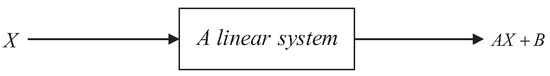
Figure 1. A linear system.

It is assumed that two model sets $M^{\left(1\right)}$ and $M^{\left(2\right)}$, where $M^{\left(1\right)}=\{m_1^{\left(1\right)},m_2^{\left(1\right)},...,m_N^{\left(1\right)}\}$ and $M^{\left(2\right)}=\{m_1^{\left(2\right)},m_2^{\left(2\right)},...,m_N^{\left(2\right)}\}$. The current motion mode is $s_k$. $M^{\left(1\right)}$ and $M^{\left(2\right)}$ are centrosymmetric and axially symmetric, respectively. However, the centers of symmetries are different. $M^{\left(1\right)}$’s center of symmetry is (0,0) and $M^{\left(2\right)}$ is $s_k$. Obviously, the connection between $M^{\left(1\right)}$ and $M^{\left(2\right)}$, as shown in Figure 2, is

$$m_i^{\left(1\right)}+s_k=m_i^{\left(2\right)},i=1,...,N$$

(6)

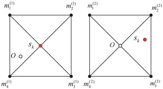
Figure 2. Example of $M^{\left(1\right)}$ and $M^{\left(2\right)}$.

For $M^{\left(1\right)}$, the distance between $s_k$ and $m_i^{\left(1\right)}$ is different, and the magnitude of the distance is

$$|m_{q^1}^{\left(1\right)}-s_k|\le |m_{q^2}^{\left(1\right)}-s_k|\le \cdots \le |m_{q^N}^{\left(1\right)}-s_k|$$

(7)

For IMM algorithm, the connection between the model probability $u^{\left(i\right)}$ and the distance $|m^{\left(i\right)}-s_k|$ is

$$|m^{\left(i\right)}-s_k|\propto \frac{1}{u^{\left(i\right)}}$$

(8)

Then, the following relation can be determined as

$$u_{q^1}^{\left(1\right)}\le u_{q^2}^{\left(1\right)}\le ...\le u_{q^N}^{\left(1\right)}$$

(9)

For each model $m_i^{\left(1\right)}$, they have different errors ${\widehat{x}}_{k|k}^{\left(i\right)|M^{\left(1\right)}}-s_k={\delta }_i^{\left(1\right)}$; thus, the overall estimation error is

$$ERRO{R}^{\left(1\right)}=\sum _i{u}_i^{\left(1\right)}{\delta }_i^{\left(1\right)}$$

(10)

Clearly, according to (8), the overall estimation error has been reduced to a certain extent. However, since the system is linear and it is asymmetrical with respect to $s_k$, the error of each $m_i^{\left(1\right)}$ is not eliminated well.

Since $M^{\left(2\right)}$ holds symmetric properties, the relationships can be obtained as

$$\left\{\begin{array}{c}\begin{array}{c}{m}_{p_1^{\left(1\right)}}^{\left(2\right)}-s_k=\cdots =m_{p_1^{(2/N_1)}}^{\left(2\right)}-s_k\hfill \\ =s_k-m_{p_1^{(2/N_1+1)}}^{\left(2\right)}\cdots =s_k-m_{p_1^{\left(N_1\right)}}^{\left(2\right)}={\delta }_{p_1}^{\left(2\right)}\hfill \end{array}\hfill \\ \begin{array}{c}⋮\hfill \\ m_{p_i^{\left(1\right)}}^{\left(2\right)}-s_k=\cdots =m_{p_i^{(2/N_i)}}^{\left(2\right)}-s_k\hfill \\ =s_k-m_{p_i^{(2/N_i+1)}}^{\left(2\right)}\cdots =s_k-m_{p_i^{\left(N_i\right)}}^{\left(2\right)}={\delta }_{p_i}^{\left(2\right)}\hfill \end{array}\hfill \\ ⋮\hfill \\ \begin{array}{c}{m}_{p_n^{\left(1\right)}}^{\left(2\right)}-s_k=\cdots =m_{p_n^{(2/N_n)}}^{\left(2\right)}-s_k\hfill \\ =s_k-m_{p_n^{(2/N_n+1)}}^{\left(2\right)}\cdots =s_k-m_{p_n^{\left(N_n\right)}}^{\left(2\right)}={\delta }_{p_n}^{\left(2\right)}\hfill \end{array}\hfill \end{array}\right.$$

(11)

where $N={\displaystyle \sum _i}{N}_i$, and $N_i$ is even number. In this linear system, $m_{p_j^{\left(i\right)}}^{\left(2\right)}$ and $m_{p_j^{(i+N_j/2)}}^{\left(2\right)}$ produce two opposite errors ${\epsilon }_{p_j}^{\left(2\right)}$ and $-{\epsilon }_{p_j}^{\left(2\right)}$, and

$$\begin{array}{c}{\epsilon }_{p_j}^{\left(2\right)}=x_{k|k}^{\left(p_j\right)|M^{\left(2\right)}}-s_k\hfill \\ -{\epsilon }_{p_j}^{\left(2\right)}=x_{k|k}^{\left(p_{j+N_j/2}\right)|M^{\left(2\right)}}-s_k\hfill \end{array}$$

(12)

Theoretically, if $M^{\left(2\right)}$ is strictly symmetric with respecting to $s_k$, the overall errors are equal to 0, without considering the system noise.

3.2. Proportional Reduction Optimization Method

Suppose two model sets $M^{\left(1\right)}=\{m_1^{\left(1\right)},m_2^{\left(1\right)},...,m_N^{\left(1\right)}\}$ and $M^{\left(2\right)}=\{m_1^{\left(2\right)},m_2^{\left(2\right)},...,m_N^{\left(2\right)}\}$, and the current model is $s_k$. The relationship between $M^{\left(1\right)}$ and $M^{\left(2\right)}$ is

$$\frac{m_i^{\left(1\right)}-s_k}{m_i^{\left(2\right)}-s_k}=\alpha >1$$

(13)

Then, the model sets obeying the equation above can be called relative position invariant model sets. The most important feature is that the position of the model sets relative of $s_k$ does not change, as shown in Figure 3.

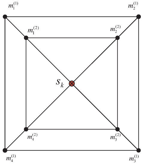
Figure 3. Topology structure of $M^{\left(1\right)}$ and $M^{\left(2\right)}$.

It is obvious that $M^{\left(2\right)}$ is more likely to have better performance than $M^{\left(1\right)}$. However, the precondition is that the topology formed by $M^{\left(1\right)}$ includes all possible real models, as shown in Figure 4. If the topology is tangent to the true mode space S, this situation can be called the critical point, namely, $\alpha ={\alpha }_0$.

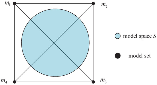
Figure 4. Topology of a model set including all model space S.

Thus, if some noise could be tolerated, the following relationships are determined as

$$\left\{\begin{array}{c}{u}_1^{\left(1\right)}=u_1^{\left(2\right)}\\ u_2^{\left(1\right)}=u_2^{\left(2\right)}\\ ⋮\\ u_N^{\left(1\right)}=u_N^{\left(2\right)}\end{array}\right.$$

(14)

For IMM, the distance between $m_i$ and $s_k$ directly affects the final error

$$|m_i-s_k|\propto |{\widehat{x}}_{k|k}^{\left(i\right)}-s_k|$$

(15)

From (13), if the value of $\alpha$ is suitable, it is easy to deduce as

$$|{\widehat{x}}_{k|k}^{\left(i\right)|M^{\left(2\right)}}-s_k|<|{\widehat{x}}_{k|k}^{\left(i\right)|M^{\left(1\right)}}-s_k|$$

(16)

The connection between overall estimation error of $M^{\left(1\right)}$ and $M^{\left(2\right)}$ is

$$|ERRO{R}^{\left(2\right)}|<|ERRO{R}^{\left(1\right)}|$$

(17)

Generally, if the model set is scaled down, its performance improves. However, the scale should not be too small, or even exceed the critical point; otherwise, it may make the covariance matrix irreversible.

3.3. Expected Model Optimization Method

If the theories referenced in Section 3.1 and Section 3.2 is feasible, the common condition is: the current model $s_k$ is known or a model is found to approach $s_k$ as close as possible. Then, an effective method to approach the current model $s_k$, called expected-mode augmentation, is given in [31]. The current expected model $m_e$ is the weighted sum of all the models at the current time

$$m_e=\sum _i{u}_i{m}_i$$

(18)

and it is closer than any model to $s_k$, namely, $|m_e-s_k|<min\{|m_1-s_k|,|m_2-s_k|,...,|m_N-s_k\left|\right\}$. However, the value of $|m_e-s_k|$ is not small enough, as shown in Figure 5. Expected model $m_e$ may appear in anywhere in expected model space. If $m_e+\gamma =s_k$, where $\gamma$ is the error, it is necessary to find a method to reduce $\gamma$ to a certain extent.

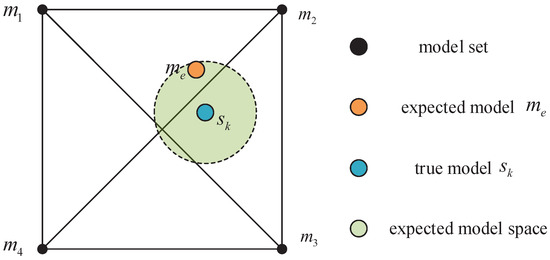
Figure 5. Example of the mentioned hypothesis.

If $m_e$ is scaled a little bit, let $m_e$ becomes $\lambda m_e$, where $\lambda$ is scaling factor. Thus, (18) is rewritten as

$$s_k-\lambda m_e=\gamma -(\lambda -1)m_e$$

(19)

and the conditions are

$$\left\{\begin{array}{c}\lambda >1,\gamma <0\hfill \\ 0<\lambda <1,\gamma >0\hfill \end{array}\right.$$

(20)

Obviously, the error $\gamma$ reduces to $\gamma -(\lambda -1)m_e$. If $\lambda$ is chosen reasonably, the error becomes small enough and $\lambda m_e$ becomes close enough to $s_k$, namely, $\frac{\lambda m_e-s_k}{\lambda m_e+s_k}\approx 0$. What is worth noting is increasing or decreasing $\lambda$ blindly contributes to serious mistakes, including even worse performance.

4. Variable Structure of Interacting Multiple-Model Algorithm Aided by Center Scaling

In this section, we introduce a new VSIMM algorithm: VSIMM-CS. The Section 3.1, Section 3.2 and Section 3.3 provide three model optimization theories. The main idea of VSIMM-CS is finding the $\lambda m_e$ to approach the current real model $s_k$ as close as possible, and moving the original model set M and scaling it to obtain the current model set $M^{\left(k\right)}$. The current model set $M^{\left(k\right)}$ could achieve better performance than the original model set M. The main function of the original model set M is locating the expected model $m_e$.

The VSIMM algorithm has a clear framework of inputs and outputs. The process of Section 2.2 can be denoted as

$$\begin{array}{c}VSIMM[M^{(k-1)},M^{\left(k\right)}]:\hfill \\ \{{\widehat{x}}_{k|k}^{i|M^{\left(k\right)}},p_{k|k}^{i|M^{\left(k\right)}},u_{k|k}^{i|M^{\left(k\right)}}\}\hfill \\ =VSIMM({\widehat{x}}_{k-1|k-1}^{i|M^{(k-1)}},p_{k-1|k-1}^{i|M^{(k-1)}},u_{k-1|k-1}^{i|M^{(k-1)}})\hfill \end{array}$$

(21)

Obviously, if $M^{\left(k\right)}=M^{(k-1)}$, the processing becomes to FIMM. Thus, the FIMM is a special case of VSIMM.

$$\begin{array}{c}FIMM\left[M\right]:\hfill \\ \{{\widehat{x}}_{k|k}^{i|M},p_{k|k}^{i|M},u_{k|k}^{i|M}\}\hfill \\ =FIMM({\widehat{x}}_{k-1|k-1}^{i|M},p_{k-1|k-1}^{i|M},u_{k-1|k-1}^{i|M})\hfill \end{array}$$

(22)

The novel VSIMM-CS always has an original model set M, which is taken part in the whole processing of target tracking, and $M^{\left(k\right)}$ is always generated by M. $M^{\left(k\right)}$ and $M^{(k-1)}$ are probably completely different. The steps of VSIMM-CS are shown in Algorithm 1.

Algorithm 1 VSIMM-CS Process

S1: Increase the time counter k by 1. S2: Run the $FIMM\left[M\right]$ cycle, and obtain the outputs: ${\widehat{x}}_{k+1|k+1}^i$,$u_{k+1|k+1}^i$ and $p_{k+1|k+1}^i$, based on the model set M. S3: Obtain the expected model $m_e$ by using EMA algorithm, which is the weighted summation of all models. $$m_e={\sum }_i{u}_{k+1|k+1}^i{m}_i$$ S4: Select the suitable values of $\alpha$ and $\lambda$ to generate the current model set $M^{(k+1)}$. $M^{(k+1)}=\alpha \{m_i+\lambda m_e,i=1,2,...,N\}$ S5: Run the $VSIMM[M^{\left(k\right)},M^{(k+1)}]$ cycle to obtain the final results. $${\widehat{x}}_{k+1|k+1}=\sum _{m^{\left(i\right)}\in M^{(k+1)}}{\widehat{x}}_{k+1|k+1}^{\left(i\right)|M^{(k+1)}}{u}_k^{\left(i\right)|M^{(k+1)}}$$ $$\begin{array}{cc}{p}_{k+1|k+1}=& {\displaystyle \sum _{m^{\left(i\right)}\in M^{(k+1)})}}[p_{k+1|k+1}^{\left(i\right)|M^{(k+1)}}+({\widehat{x}}_{k+1|k+1}^{\left(i\right)|M^{(k+1)}}-{\widehat{x}}_{k+1|k+1})\\ & {({\widehat{x}}_{k+1|k+1}^{\left(i\right)|M_{(k+1)}}-{\widehat{x}}_{k+1|k+1})}^{\prime }]u_{k+1|k+1}^{\left(i\right)|M^{(k+1)}}\hfill \end{array}$$ S6: Go to $\mathbf{S}\mathbf{1}$.

The algorithm complexity is $T\left(n\right)=2n^2+16n$, and n equals to the number of models.

The most important part of the process is model set generation. The values of $\lambda$ and $\alpha$ have a huge impact on the performance of the model set. Therefore, it is unreasonable to choose $\lambda$ and $\alpha$ blindly. The biggest advantage of VSIMM-CS is that the model set is generated in real-time without increasing huge computational complexity. In addition, if the original model set is designed rational and the number of models is few, the proposed VSIMM-CS can achieve rewarding results and keep the calculation volume within a reasonable range at the same time. The rational combination of $\lambda$ and $\alpha$ achieve great performance in terms of precision.

5. Simulation Results

In this section, a reasonable simulation process is given: firstly, the target state, the measurement equations and their specific parameters are presented. Secondly, the original model set is given, including the probability transition matrix. Thirdly, the target motion state and performance criterion are presented. Finally, different simulation results are analyzed.

The target state and the measurement equations are, respectively, given as

$$x_{k+1}=F_k^{\left(j\right)}{x}_k+G_k^{\left(j\right)}{a}_k^{\left(j\right)}+w_k^{\left(j\right)}$$

(23)

$$z_k=H_k^{\left(j\right)}{x}_k+v_k^{\left(j\right)}$$

(24)

where $w_k^{\left(j\right)}\sim N[0,0.01]$; $v_k^{\left(j\right)}\sim N[0,1250]$; $a_k^{\left(i\right)}$ is target acceleration input;

$F=\left[\begin{array}{cccc}1& T& 0& 0\\ 0& 1& T& 0\\ 0& 0& 1& T\\ 0& 0& 0& 1\end{array}\right]$ and $G={\left[\begin{array}{cccc}0.5\hfill & 1& 0& 0\\ 0\hfill & 0& 0.5& 1\end{array}\right]}^{\prime }$. T is time interval.

The original model set M included 4 models as

$$\left\{\begin{array}{cc}{m}_1={[-10,10]}^{\prime }& m_2={[10,10]}^{\prime }\\ m_4={[-10,-10]}^{\prime }& m_3={[10,-10]}^{\prime }\end{array}\right\}$$

(25)

and its topology structure is shown in Figure 6

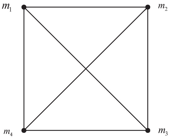
Figure 6. Topology structure of M.

Its probability transition matrix $\mathrm{\Pi }$ is $\left[\begin{array}{cccc}0.85& 0.05& 0.05& 0.05\\ 0.05& 0.85& 0.05& 0.05\\ 0.05& 0.05& 0.85& 0.05\\ 0.05& 0.05& 0.05& 0.85\end{array}\right]$. The Table 1 illustrates an ensemble of maneuver trajectories for compare the existing and proposed algorithm.

Table 1. Parameters of deterministic scenarios.

Time k (s)	${\mathit{a}}_{\mathit{x}}$ (m/s2)	${\mathit{a}}_{\mathit{y}}$ (m/s2)
1–50	0	0
50–100	5	5
100–150	3	$-7$
150–200	7	$-2$
200–250	4	1
250–300	$-4$	$-2$
300–350	0	0

If $\overline{e}$ represents the average error of the whole processing, it can be denoted as

$$\overline{e}=\sum _{k=k_1}^{k_N}\sqrt{\left({\left({\widehat{x}}_k-x_k\right)}^{\prime }\left[\begin{array}{cccc}1& 0& 0& 0\\ 0& 0& 0& 0\\ 0& 0& 1& 0\\ 0& 0& 0& 0\end{array}\right]\right)\ast \left(\left[\begin{array}{cccc}1& 0& 0& 0\\ 0& 0& 0& 0\\ 0& 0& 1& 0\\ 0& 0& 0& 0\end{array}\right]\left({\widehat{x}}_k-x_k\right)\right)}/\left(k_N-k_1\right)$$

(26)

where ${\widehat{x}}_k$ is the best estimation at time k, $x_k$ is the target state; and $N=300$. Therefore, different $\lambda$ and $\alpha$ produce different $\overline{e}$, as shown in Table 2. The unit of $\overline{e}$ is meters, and we just consider the position error.

Table 2. The average error $\overline{e}$ of the tracking process.

	α	0.5	0.6	0.7	0.8	0.9
λ
0.8		16.72	13.00	10.45	8.59	7.19
1.9		13.29	9.89	7.55	5.84	4.56
3		10.16	6.96	4.76	3.15	1.98
4.1		7.21	4.16	2.09	0.98	1.52
5.2		4.32	1.53	1.86	3.14	4.09

Different combinations of $\lambda$ and $\alpha$ present different performances. Assume $\lambda =0.8,1.9,3,4.1,5.2$ and $\alpha =0.5,0.6,0.7,0.8,0.9$. Their root mean square errors (RMSE) are shown in Figure 7 with 50 times Montecarlo experiment.

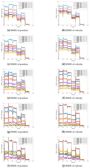
Figure 7. Root mean square error of VSIMM-CS.

In most cases, the VSIMM-CS shows great performance on target tracking, and its errors are far lower than FIMM using 4 models. In some cases, the error is close to 0, and the proposed VSIMM-CS achieves a perfect performance. Thus, sacrificing a certain amount of computation for high accuracy is an acceptable approach.

When $\lambda =0.8$, as shown in Figure 7a,b, most values of $\alpha$ do not present better performance than IMM-4. Especially, when $\alpha =0.5$, it becomes the worst one and it produces twice as many errors as IMM-4. As $\alpha$ is increasing, the errors reduce gradually. Until $\alpha =0.8$, the error curve is as same as IMM-4. When $\alpha =0.9$, it becomes better than IMM-4. Obviously, in the situation of $\lambda =0.8$, VSIMM-CS does not show its high precision. When $\lambda =1.9$ in Figure 7c,d, compared with $\lambda =0.8$, the tracking precision has been improved. Noting that when $\alpha =0.7$ or $0.8$, the errors are smaller than IMM-4. However, when $\alpha =0.5$, it is still the worst one among them. It is surprising that, except $\alpha =0.5$ when $\lambda =3$, other values of $\alpha$ have greater performance than IMM-4. The relationship of these five algorithms has not changed. $\alpha =0.9$ is still the best one and $\alpha =0.5$ is still the worst one. Only when $\alpha =0.5$, the performance is worse than IMM-4. While the minimum position error is about two meters, it is not close enough to 0. Clearly, up to now, $\lambda$ does not achieve the most suitable value. When $\lambda =4.1$, all VSIMM-CS algorithms have better performance than IMM-4, even $\alpha =0.5$, $\alpha =0.7$, and $\alpha =0.9$ have similar tracking precision, and $\alpha =0.9$ is not the best one anymore. When $\alpha =0.7$, the position error is smaller than that in any situation as shown in Figure 7. When the true model does not equal to ${(0,0)}^{\prime }$, the position error is also very close to 0. It seems that the best combination is $\lambda =4.1$ and $\alpha =0.8$ in this system. In this case, the conclusion, referenced in Section 3, has been fully demonstrated. As shown in Figure 7i,j, VSIMM-CS still shows its great performance. All the error curves are less than half of IMM-4’s, and $\alpha =0.6$ has the highest accuracy. The simulation result of $\alpha =0.7$ is very close to $\alpha =0.6$. However, the best one shown in Figure 7g,h does not maintain its advantage in Figure 7i,j.

For $\alpha =0.5$, as $\lambda$ changes, its precision does not become better, except $\lambda <5.2$. In these simulation results, it is always the worst one among VSIMM-CS algorithms. The main reason for this is that the value of $\alpha$ is too small. Similarly, $\alpha =0.6$ still does not meet the requirements. Compared with $\alpha =0.5$, its performance becomes better. It is not difficult to find that VSIMM-CS takes twice as much computation as IMM-4. However, in most cases, the promotion of $\alpha =0.6$ is very limited, even it is worse than IMM-4 when $\lambda =0.9$ or $1.9$. Only when $\lambda =5.2$ does it have the best performance, which is shown in Figure 7i,j. When $\alpha =0.7$, the precision becomes acceptable. Though it is not the best one in all situations, the performance is greatly promoted. As $\lambda$ increases, the tracking precision of the proposed algorithm becomes better. When $\alpha =0.8$ and $\lambda \le 3$, it only performs worse than $\alpha =0.9$. Especially when $\lambda =4.1$, its performance becomes the best one. However, if the value of $\lambda$ is too large, referenced as Figure 7ij, its advantage disappears. When $\alpha =0.9$, its performance is always the best one in Figure 7a–f. Similarly, when $\lambda =5.2$, so much large value of $\lambda$ would deteriorate the performance.

A good demonstration of the average error $\overline{e}$ of the unworkable portfolio is shown in Table 2. If $\alpha <0.7$, the critical point would not bee meet the condition at certain times. When $\alpha =0.7,0.8,0.9$, respectively, there is a high probability that the proposed algorithm achieves better performance.

In general, VSIMM-CS certainly achieves a big performance boost compared with FIMM, if $\lambda$ and $\alpha$ are selected rationally. Different systems tend to have different suitable combinations of $\lambda$ and $\alpha$. Smaller $\alpha$ or larger $\lambda$ do not promote the performance. According to the current system, the reasonable $\lambda$ and $\alpha$ always reflect satisfactory results.

6. Conclusions

In this paper, a new variable structure interacting multiple-model algorithm, VSIMM-CS, is proposed. Its model set is generated in real-time, and the generated model set is based on the original model set. Considering the error properties of a linear system and the symmetry of model set structure, the two theories called proportional reduction optimization method and symmetric model set optimization method are presented. The main purpose of the two theories is to reduce errors. Without considering the effect of noise, VSIMM-CS eliminates errors perfectly. To better locate the real model, the expected model optimization method is proposed. The excepted model generated by this method is closer than any other model. Simulation results show different combinations of $\alpha$ and $\lambda$ have different performances. In most cases, VSIMM-CS achieved better tracking results. It is acceptable to sacrifice a certain amount of computation for high accuracy. A huge performance boost can be obtained by the precise selection of $\alpha$ and $\lambda$. When the performance achieves in the optimal situation, $\alpha$ and $\lambda$ are 0.8 and 4.1, respectively. In different simulation conditions, the results may be different. Many factors may influence the values of $\alpha$ and $\lambda$, such as noise, original model set, and true mode space, etc., and our following research aims to focus on these factors. However, the unreasonable selection of $\alpha$ and $\lambda$ leads to worse results. Simulation results also highlight the rationality and feasibility of this novel approach.

References

- Gorji, A.A.; Tharmarasa, R.; Kirubarajan, T. Performance measures for multiple target tracking problems. In Proceedings of the 14th International Conference on Information Fusion, Chicago, IL, USA, 5–8 July 2011; pp. 1–8. [Google Scholar]
- Poore, A.B.; Gadaleta, S. Some assignment problems arising from multiple target tracking. Math. Comput. Model. 2006, 43, 1074–1091. [Google Scholar] [CrossRef]
- Huang, X.; Tsoi, J.K.; Patel, N. mmWave Radar Sensors Fusion for Indoor Object Detection and Tracking. Electronics 2022, 11, 2209. [Google Scholar] [CrossRef]
- Wei, Y.; Hong, T.; Kadoch, M. Improved Kalman filter variants for UAV tracking with radar motion models. Electronics 2020, 9, 768. [Google Scholar] [CrossRef]
- Li, X.R.; Bar-Shalom, Y. Multiple-model estimation with variable structure. IEEE Trans. Autom. Control 1996, 41, 478–493. [Google Scholar]
- Magill, D. Optimal adaptive estimation of sampled stochastic processes. IEEE Trans. Autom. Control 1965, 10, 434–439. [Google Scholar] [CrossRef]
- Lainiotis, D. Optimal adaptive estimation: Structure and parameter adaption. IEEE Trans. Autom. Control 1971, 16, 160–170. [Google Scholar] [CrossRef]
- Tudoroiu, N.; Khorasani, K. Satellite fault diagnosis using a bank of interacting Kalman filters. IEEE Trans. Aerosp. Electron. Syst. 2007, 43, 1334–1350. [Google Scholar] [CrossRef]
- Kirubarajan, T.; Bar-Shalom, Y.; Pattipati, K.R.; Kadar, I. Ground target tracking with variable structure IMM estimator. IEEE Trans. Aerosp. Electron. Syst. 2000, 36, 26–46. [Google Scholar] [CrossRef]
- Grossman, R.L.; Nerode, A.; Ravn, A.P.; Rischel, H. Hybrid Systems; Springer: Berlin/Heidelberg, Germany, 1993; Volume 736. [Google Scholar]
- Branicky, M.S. Introduction to hybrid systems. In Handbook of Networked and Embedded Control Systems; Birkhäuser: Basel, Switzerland, 2005; pp. 91–116. [Google Scholar]
- Li, X.R. Multiple-model estimation with variable structure. II. Model-set adaptation. IEEE Trans. Autom. Control 2000, 45, 2047–2060. [Google Scholar]
- Labbe, R. Kalman and bayesian filters in python. Chap 2014, 7, 4. [Google Scholar]
- Zhang, G.; Lian, F.; Gao, X.; Kong, Y.; Chen, G.; Dai, S. An Efficient Estimation Method for Dynamic Systems in the Presence of Inaccurate Noise Statistics. Electronics 2022, 11, 3548. [Google Scholar] [CrossRef]
- Rong Li, X.; Jilkov, V. Survey of maneuvering target tracking. Part V. Multiple-model methods. IEEE Trans. Aerosp. Electron. Syst. 2005, 41, 1255–1321. [Google Scholar] [CrossRef]
- Bar-Shalom, Y. Multitarget-Multisensor Tracking: Applications and Advances; Artech House, Inc.: Norwood, MA, USA, 2000; Volume iii. [Google Scholar]
- Blom, H.A.; Bar-Shalom, Y. The interacting multiple model algorithm for systems with Markovian switching coefficients. IEEE Trans. Autom. Control 1988, 33, 780–783. [Google Scholar] [CrossRef]
- Ma, Y.; Zhao, S.; Huang, B. Multiple-Model State Estimation Based on Variational Bayesian Inference. IEEE Trans. Autom. Control 2019, 64, 1679–1685. [Google Scholar] [CrossRef]
- Wang, G.; Wang, X.; Zhang, Y. Variational Bayesian IMM-filter for JMSs with unknown noise covariances. IEEE Trans. Aerosp. Electron. Syst. 2019, 56, 1652–1661. [Google Scholar] [CrossRef]
- Li, H.; Yan, L.; Xia, Y. Distributed robust Kalman filtering for Markov jump systems with measurement loss of unknown probabilities. IEEE Trans. Cybern. 2021, 52, 10151–10162. [Google Scholar] [CrossRef]
- Johnston, L.; Krishnamurthy, V. An improvement to the interacting multiple model (IMM) algorithm. IEEE Trans. Signal Process. 2001, 49, 2909–2923. [Google Scholar] [CrossRef]
- Fan, X.; Wang, G.; Han, J.; Wang, Y. Interacting Multiple Model Based on Maximum Correntropy Kalman Filter. IEEE Trans. Circuits Syst. II Express Briefs 2021, 68, 3017–3021. [Google Scholar] [CrossRef]
- Davis, R.R.; Clavier, O. Impulsive noise: A brief review. Hear. Res. 2017, 349, 34–36. [Google Scholar] [CrossRef]
- Nie, X. Multiple model tracking algorithms based on neural network and multiple process noise soft switching. J. Syst. Eng. Electron. 2009, 20, 1227–1232. [Google Scholar]
- Mazor, E.; Averbuch, A.; Bar-Shalom, Y.; Dayan, J. Interacting multiple model methods in target tracking: A survey. IEEE Trans. Aerosp. Electron. Syst. 1998, 34, 103–123. [Google Scholar] [CrossRef]
- Gao, W.; Wang, Y.; Homaifa, A. Discrete-time variable structure control systems. IEEE Trans. Ind. Electron. 1995, 42, 117–122. [Google Scholar]
- Li, X.R.; Bar-Shakm, Y. Mode-set adaptation in multiple-model estimators for hybrid systems. In Proceedings of the 1992 American Control Conference, Chicago, IL, USA, 24–26 June 1992; pp. 1794–1799. [Google Scholar]
- Pannetier, B.; Benameur, K.; Nimier, V.; Rombaut, M. VS-IMM using road map information for a ground target tracking. In Proceedings of the 2005 7th International Conference on Information Fusion, Philadelphia, PA, USA, 25–28 July 2005; Volume 1. 8p. [Google Scholar]
- Xu, L.; Li, X.R. Multiple model estimation by hybrid grid. In Proceedings of the 2010 American Control Conference, Baltimore, MD, USA, 30 June–2 July 2010; pp. 142–147. [Google Scholar]
- Li, X.R.; Zwi, X.; Zwang, Y. Multiple-model estimation with variable structure. III. Model-group switching algorithm. IEEE Trans. Aerosp. Electron. Syst. 1999, 35, 225–241. [Google Scholar]
- Li, X.R.; Jilkov, V.P.; Ru, J. Multiple-model estimation with variable structure-part VI: Expected-mode augmentation. IEEE Trans. Aerosp. Electron. Syst. 2005, 41, 853–867. [Google Scholar]
- Lan, J.; Li, X.R. Equivalent-Model Augmentation for Variable-Structure Multiple-Model Estimation. IEEE Trans. Aerosp. Electron. Syst. 2013, 49, 2615–2630. [Google Scholar] [CrossRef]
- Li, X.R.; Zhang, Y. Multiple-model estimation with variable structure. V. Likely-model set algorithm. IEEE Trans. Aerosp. Electron. Syst. 2000, 36, 448–466. [Google Scholar]
- Sun, F.; Xu, E.; Ma, H. Design and comparison of minimal symmetric model-subset for maneuvering target tracking. J. Syst. Eng. Electron. 2010, 21, 268–272. [Google Scholar] [CrossRef]
- Callier, F.M.; Desoer, C.A. Linear System Theory; Springer Science & Business Media: Berlin, Germany, 2012. [Google Scholar]
- Kalman, R.E. A new approach to linear filtering and prediction problems. J. Basic Eng. 1960, 82, 35–45. [Google Scholar] [CrossRef]
Disclaimer/Publisher’s Note: The statements, opinions and data contained in all publications are solely those of the individual author(s) and contributor(s) and not of MDPI and/or the editor(s). MDPI and/or the editor(s) disclaim responsibility for any injury to people or property resulting from any ideas, methods, instructions or products referred to in the content. |
© 2023 by the authors. Licensee MDPI, Basel, Switzerland. This article is an open access article distributed under the terms and conditions of the Creative Commons Attribution (CC BY) license (https://creativecommons.org/licenses/by/4.0/).