Solutions of the Yang–Baxter Equation Arising from Brauer Configuration Algebras

Abstract

Currently, researching the Yang–Baxter equation (YBE) is a subject of great interest among scientists of diverse areas in mathematics and other sciences. One of the fundamental open problems is to find all of its solutions. The investigation deals with developing theories such as knot theory, Hopf algebras, quandles, Lie and Jordan (super) algebras, and quantum computing. One of the most successful techniques to obtain solutions of the YBE was given by Rump, who introduced an algebraic structure called the brace, which allows giving non-degenerate involutive set-theoretical solutions. This paper introduces Brauer configuration algebras, which, after appropriate specializations, give rise to braces associated with Thompson’s group F. The dimensions of these algebras and their centers are also given.

1. Introduction

The Yang–Baxter equation (YBE) arose from research in theoretical physics and statistical mechanics. On the one hand, Yang [1] introduced in 1967 such an equation in two short papers regarding generalizations of the results obtained by Lieb and Liniger. Using the Bethe ansatz, they solved the one-dimensional repulsive Bose gas with delta function interaction. On the other hand, Baxter [2] solved the eight-vertex ice model in 1971, introduced previously by Lieb. Baxter’s method was based on commuting transfer matrices starting from a solution called by him the generalized star–triangle equation, which currently is known as the Yang–Baxter equation [3,4].

It is worth pointing out that finding a complete classification of the YBE solutions remains an open problem. However, to date, many solutions have been found to this equation. Research on this subject can be considered a trending topic. It has encouraged investigations in several science fields. For instance, the YBE has had an important role in developing Hopf algebras, Yetter–Drinfeld categories, quandles, knot theory, cluster algebras (via the Jones polynomial of a two-bridge knot), braided categories, group action relations on sets, quantum computing, cryptography, etc. [5,6,7,8,9].

Another strategy to tackle the problem of classifying some types of the YBE was introduced by Rump [10,11], who introduced the notion of the brace. Braces allow classifying so-called non-degenerate involutive set-theoretical solutions of the YBE. In particular, Ballester-Bolinches et al. [12] proved how it is possible to obtain a left brace $\left(\mathcal{G}\right(X,r),+,.)$ structure from the Cayley graph of a suitable subgroup of the symmetric group $\mathrm{Sym}\left(X\right)$ associated with a set X defining a solution $(X,r)$ of the YBE.

On the other hand, Brauer configuration algebras (BCAs) are bound quiver algebras [13] induced by configurations of appropriate multisets called Brauer configurations. The combinatorial data arising from these configurations provide information on the theory of representations of their corresponding Brauer configuration algebras. As in the case of the YBE, BCAs have proven to be a tool for developing different science fields. They have been used in cryptography to give an algebraic interpretation of the Advanced Encryption Standard (AES) key schedule, in the theory of graph energy to compute the trace norm of some families of matrices and trees, in coding theory to compute the energy of a code, etc. [14,15,16].

It is worth noting that Espinosa [17] proved that to be associated with a Brauer configuration. There is a message obtained by concatenating appropriate words defining their multisets named polygons by Green and Schroll [13]. Espinosa defined specializations for these messages, making them elements of suitable algebraic structures (rings, groups, etc.). Such a procedure allows new interpretations of objects and morphisms in different categories.

1.1. Motivations

Researching the classification of the YBE solutions is one of the trending topics in mathematics and its applications. Results regarding the subject involve areas such as cryptography, quantum computing, group theory, Hopf algebras, and Lie (super) algebras, among others [5,6,7,8,9]. On the other hand, Brauer configuration algebras have helped investigate the theory of graph energy, cryptography, and coding theory [14,15,16]. This work connects the Brauer configuration algebras theory with the YBE theory by introducing Brauer configurations whose specializations give rise to braces, which provide solutions to the YBE.

1.2. Contributions

This paper introduces brace families arising from appropriate Brauer configuration algebras. The dimensions of these algebras and their centers are also computed. According to Rump’s results, the obtained braces give rise to non-degenerate involutive set-theoretical solutions of the YBE.

Figure 1 shows how Brauer configuration algebras and brace theories are related to obtaining the main results presented in this paper (see the targets of red arrows).

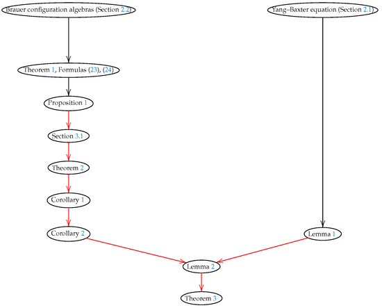
Figure 1. Main results presented in this paper (targets of red arrows) allow establishing a connection between Brauer configuration algebras and YBE theories.

Section 3.1 introduces Brauer configuration algebras of type ${\mathfrak{F}}^{(i,j,k)}$.

Theorem 2 proves that algebras of type ${\mathfrak{F}}^{(i,j,k)}$ are reduced and connected. Corollary 1 gives formulas for the dimensions of algebras ${\mathfrak{F}}^{(i,j,k)}$ and their centers. Corollary 2 proves that these Brauer configuration algebras have length grading induced by the associated path algebra as a consequence of Proposition 1.

Lemma 2 proves that messages associated with Brauer configurations of type ${\mathfrak{F}}^{(i,j,k)}$ induce a subgroup of Thompson’s group of type F. This lemma is used to prove that such a subgroup endowed with an appropriate sum constitute a brace, which can be used to generate non-degenerate involutive set-theoretical solutions of the YBE.

The organization of this paper is as follows. The main definitions and notation are given in Section 2. In particular, we recall the notions of the YBE, braces, and Brauer configuration algebra (Section 2.2). In Section 3, we give our main results. We introduce Brauer configurations of type ${\mathfrak{F}}^{(i,j,k)}$ (Section 3.1), and it is proven that the corresponding algebras are reduced, indecomposable, and have length grading induced by the associated path algebra. It is also proven that messages associated with these Brauer configurations give rise to some braces, therefore to some solutions of the YBE. Concluding remarks are given in Section 4.

2. Background and Related Work

This section reminds about the basic notation and results regarding the YBE, braces, and Brauer configuration algebras, which are helpful for a better understanding of the paper.

2.1. Yang–Baxter Equation and Its Solutions

In this section, we give a brief review on the Yang–Baxter equation and some of the methods used to solve it [4,5,6,10,12].

Let V be a vector space over an algebraically closed field $\mathbb{F}$ of characteristic zero. A linear automorphism R of $V\otimes V$ is a solution of the Yang–Baxter equation (sometimes called the braided relation), if the following identity (1) holds

$$(R\otimes id)\circ (id\otimes R)\circ (id\otimes R)=(id\otimes R)\circ (R\otimes id)\circ (R\otimes id).$$

(1)

in the automorphism group $V\otimes V\otimes V$.

R is a solution of the quantum Yang–Baxter equation if

$$R_{12}\circ R_{13}\circ R_{23}=R_{23}\circ R_{13}\circ R_{12}$$

(2)

where $R_{ij}$ means R acting on the ith and jth tensor factor and as the identity on the remaining factor.

To date, finding a complete classification of all the solutions of the YBE is an open problem. However, several approaches have been explored to obtain solutions of these equations. For instance, Drinfeld et al. [18] proposed studying set-theoretical solutions of the YBE; in such a case, for a given set X and a map $S:X\times X\to X\times X$, the identity (1) has the form

$$(S\times id)\circ (id\times S)\circ (S\times id)=(id\times S)\circ (S\times id)\circ (id\times S),$$

(3)

in $X\times X\times X$.

Note that, if $\tau :X^2\to X^2$ is defined in such a way that $\tau (x,y)=(y,x)$, then a map $S:X^2\to X^2$ is a set-theoretical solution of the YBE if and only if $r=\tau \circ S$ is a solution of the following braided equation:

$$r_{12}{r}_{23}{r}_{12}=r_{23}{r}_{12}{r}_{23}.$$

(4)

A bijective map $r:X\times X\to X\times X$, such that $r(x,y)=({\sigma }_x\left(y\right),{\gamma }_y\left(x\right))$ is involutive if $r^2=i{d}_{X^2}$. r is said to be left non-degenerate (right non-degenerate), if each map ${\gamma }_x$ (${\sigma }_x$) is bijective.

Note that, if X is finite, then an involutive solution of the braided equation is right non-degenerate if and only if it is left non-degenerate. It is worth noticing that non-degenerate involutive set-theoretical solutions of the YBE were given by Etingof et al. [19] and Gateva-Ivanova and Van den Bergh [20] by associating a group $G(X,r)$ with the solution $(X,r)$ [4].

Rump [10] introduced another line of investigation to tackle the problem of classifying the non-degenerate involutive set theoretical solutions of the YBE. To do that, he defined right braces and left braces. A right brace is a set G with two operations + and · such that:

• $(G,+)$ is an abelian group.
• $(G,·)$ is a group and

  $$(a+b)c+c=ac+bc,\mathrm{for}\mathrm{all}a,b,c\in G.$$

  (5)

$(G,+)$ is said to be the additive group and $(G,·)$ the multiplicative group of the right brace.

A left brace is defined similarly; in this case, the identity (5) has the shape

$$a(b+c)+a=ab+ac.$$

(6)

For $a\in G$, we define ${\rho }_a,{\lambda }_a\in {\mathrm{Sym}}_G$ (the symmetric group on G) by

$$\begin{array}{cc}\hfill {\rho }_a\left(b\right)& =ba-a,\hfill \\ \hfill {\lambda }_a\left(b\right)& =ab-a.\hfill \end{array}$$

(7)

Rump proved the following result.

Lemma 1

(Lemma 4.1, [4], Propositions 2 and 3 [10]). Let G be a left brace. The following properties hold:

1. 

$a{\lambda }_a^{-1}\left(b\right)=b{\lambda }_b^{-1}\left(a\right)$.

2. 

${\lambda }_a{\lambda }_{{\lambda }_a^{-1}\left(b\right)}={\lambda }_b{\lambda }_{{\lambda }_b^{-1}\left(a\right)}$.

3. 

The map $r:G\times G\to G\times G$ defined by $r(x,y)=({\lambda }_x\left(y\right),{\lambda }_{{\lambda }_x\left(y\right)}^{-1}\left(x\right))$ is a non-degenerate involutive set-theoretical solution of the YBE.

Recently, Guarnieri and Vendramin [21] generalized Rump’s work to the non-commutative setting in order to obtain not necessarily non-degenerate involutive set-theoretical solutions of the YBE. Ballester-Bolinches et al. [12] endowed a subgroup (of the symmetric group $\mathrm{Sym}\left(X\right)$) $\mathcal{G}(X,r)$ associated with a solution $(X,r)$ of the YBE with two operations + and · in such a way that the algebraic structure $\left(\mathcal{G}\right(X,r),+,·)$ is a left brace. To do that, they used the Cayley graph of $\mathcal{G}(X,r)$.

2.2. Multisets and Brauer Configuration Algebras

A multiset is a set with possibly repeated elements. To be more precise, a multiset is an ordered pair $(M,f)$, where M is a set and f is a function from M to the nonnegative integers; for each $m\in M$, $f\left(m\right)$ would be called the multiplicity of m.

According to Andrews, a permutation of a multiset $(M,f)$ is a word in which each letter belongs to M, and for each $m\in M$, the total number of appearances (or occurrences) of m in the word is $f\left(m\right)$, i.e., if M is a finite set, say $\{m_1,m_2,\dots ,m_r\}$, then a multiset $(M,f)$ can be written as a word with the form described by Identity (8).

$$(M,f)=\{m_1^{f\left(m_1\right)}{m}_2^{f\left(m_2\right)}\dots m_r^{f\left(m_r\right)}\}.$$

(8)

It is worth pointing out that, to denote multisets, the order of the elements does not matter. This condition makes the theory of multisets a source of many interesting problems in the theory of partitions assuming that $M=\{1,2,\dots ,r\}$, for an appropriate positive integer r, for instance, if $inv(m_1,m_2,\dots ,m_r;n)$ denotes the number of permutations $x_1{x}_2\dots x_{m_1+m_2\dots m_r}$ of the multiset $\{1^{m_1}{2}^{m_2}\dots r^{m_r}\}$ in which there are n pairs $(x_i,x_j)$ such that $i<j$ and $x_i>x_j$. Then, $inv(m_1,m_2;n)$ equals the number of partitions of n into at most $m_2$ parts, each $\le m_1$ [22].

An alternative notation for multisets is given by da Fontoura [23], who writes multisets in the following form:

$$(M,f)=\left\{\right|[m_1,f\left(m_1\right)],[m_2,f\left(m_2\right)],\dots ,[m_r,f\left(m_r\right)]\left|\right\}.$$

(9)

If $(M,f)$ and $(N,g)$ are multisets, then

$$\begin{array}{cc}\hfill (O,h)& =(M,f)\cup (N,g)=\left\{\right[x,h\left(x\right)]\mid x\in M\cup N,h(x)=\max \{f\left(x\right),g\left(x\right)\left\}\right\}\hfill \\ \hfill (P,i)& =(M,f)+(N,g)=\left\{\right[x,i\left(x\right)]\mid x\in M\cup N,i(x)=f(x)+g(x\left)\right\}\}\hfill \\ \hfill (R,s)& =(M,f)\cap (N,g)=\left\{\right[x,s\left(x\right)]\mid x\in M\cup N,s(x)=\min \{f\left(x\right),g\left(x\right)\left)\right\}\}.\hfill \end{array}$$

(10)

Note that, since the order of the elements does not matter, then if

$$(M_1,f_1),(M_2,f_2),\dots ,(M_n,f_n)$$

(11)

are multisets and $w(M_i,f_i)=x_{(i,1)}^{f_i\left(x_{(i,1)}\right)}{x}_{(i,2)}^{f_i\left(x_{(i,2)}\right)}\dots x_{(i,t_i)}^{f_i\left(x_{(i,t_i)}\right)}$ is the word associated with the multiset $(M_i,f_i)$, then the concatenation $w(M_1,f_1)w(M_2,f_2)\dots w(M_n,f_n)$:

$$x_{(1,1)}^{f_1\left(x_{(1,1)}\right)}{x}_{(1,2)}^{f_1\left(x_{(1,2)}\right)}\dots x_{(1,t_1)}^{f_1\left(x_{(1,t_1)}\right)}\dots x_{(n,1)}^{f_n\left(x_{(n,1)}\right)}{x}_{(n,2)}^{f_n\left(x_{(n,2)}\right)}\dots x_{(n,t_n)}^{f_n\left(x_{(n,t_n)}\right)}$$

(12)

of the words $w(M_i,f_i)$, $1\le i\le n$ is said to be the message associated with the multisets (11). It coincides with ${\displaystyle \sum _{i=1}^n}(M_i,f_i)$, if $M_i\cap M_j=⌀$ with $i\ne j$. Henceforth, if no confusion arises, we will omit brackets to denote these types of words. Note that messages associated with the same family of multisets are equivalent.

If an element $x_{(i,j)}\in M_{i_1}\cap M_{i_2}\cap \dots \cap M_{i_r}\subseteq {\displaystyle \sum _{h=1}^n}{M}_h$, then the sum ${\displaystyle \sum _{h=1}^r}{f}_{i_h}\left(x_{(i,j)}\right)$ is said to be the valency of $x_{(i,j)}$, denoted $val\left(x_{(i,j)}\right)$ [13].

For collections of labeled multisets $M_1,M_2,\dots ,M_n$ with $M_0={\displaystyle \bigcup _{h=1}^n}{M}_h$ and

$$\underset{k=1}{\sum ^{t_i}}{f}_i\left(x_{(i,k)}\right)>1,\mathrm{for}\mathrm{any}1\le i\le n\mathrm{and}{t}_i=\left|M_i\right|.$$

(13)

Green and Schroll introduced in [13] systems or configurations of multisets of the form

$$(M_0;\{M_1,M_2,\dots ,M_n\};\nu ;\mathcal{O})$$

(14)

where $\nu$ is a multiplicity map $\nu :M_0\to \mathbb{N}\times \mathbb{N}$ such that $\nu \left(x\right)=\left(val\right(x),\mu (x\left)\right)$, with $\mu \left(x\right)\ge 1$. Green and Schroll [13] called vertices the elements of $M_0$ and polygons the multisets $M_i$. According to them, a vertex $x_{(i,j)}$ is truncated provided that $\nu \left(x_{(i,j)}\right)=(1,1)$ (i.e., $val\left(x_{(i,j)}\right)\mu \left(x_{(i,j)}\right)=1$); otherwise, $x_{(i,j)}$ is said to be non-truncated. The message of the configuration is said to be reduced if, for any vertex $x_{(i,j)}\in M_0$, it holds that $\mu \left(x_{(i,j)}\right)val\left(x_{(i,j)}\right)>1$. Henceforth, we let ${\nu }_{x_{(i,j)}}$ denote the product $\mu \left(x_{(i,j)}\right)val\left(x_{(i,j)}\right)$ associated with the multiplicity of a vertex $x_{(i,j)}$ of a Brauer configuration.

The orientation $\mathcal{O}$ is obtained by defining for each non-truncated vertex $x_{(i,j)}\in M_0$ a cyclic ordering ${<}_{x_{(i,j)}}$ on the polygons $M_{i_j}$ for which $f\left(x_{(i,j)}\right)\ge 1$, i.e., if $x_{(i,j)}\in M_{i_1}\cup M_{i_2}\cup \dots M_{i_r}$, then the cyclic ordering is obtained by defining a linear order $S_{x_{(i,j)}}$ of the form

$M_{i_1}^1<M_{i_1}^2<\dots <M_{i_1}^{f_i\left(x_{(i,j)}\right)}<\dots <M_{i_r}^1<M_{i_r}^2<\dots <M_{i_r}^{f_r\left(x_{(i,j)}\right)}$ and adding a new relation $M_{i_r}^{f_r\left(x_{(i,j)}\right)}<M_{i_1}^1$. In this case, sequences of the form

$M_{i_h}^s<M_{i_h}^{s+1}<\dots <M_{i_h}^{f_h\left(x_{(i,j)}\right)}<\dots <M_{i_r}^1<M_{i_r}^2<\dots <M_{i_r}^{f_r\left(x_{(i,j)}\right)}<M_{i_1}^1<M_{i_1}^2<\dots <M_{i_h}^{s-1}$ are equivalent. Note that, for the sake of clarity, we have omitted the index $x_{(i,j)}$ for the relation ${<}_{\left(x_{(i,j)}\right)}$.

Sequences $S_{\left(x_{(i,j)}\right)}$ are said to be successor sequences.

Remark 1.

Systems of the form (14) were named Brauer configurations by Green and Schroll. In this work, it is assumed that, if $M<M^{\prime }$ in the successor sequence associated with a vertex $x\in M_0$, then if a vertex $x^{\prime }\ne x$ belongs to the polygons M and $M^{\prime }$, then $M<M^{\prime }$ in the successor sequence associated with the vertex $x^{\prime }$, i.e., the successor sequence $S_{x^{\prime }}$ inherits the order defined by the vertex x.

A Brauer configuration without truncated vertices is said to be reduced. This paper only deals with reduced Brauer configurations.

If $M=(M_0;\{M_1,M_2,\dots ,M_n\};{\nu }^M;{\mathcal{O}}^M)$, and $N=(N_0;\{N_1,N_2,\dots ,N_m\};{\nu }^N;{\mathcal{O}}^N)$ are Brauer configurations, then the Brauer configuration:

$$P=M+N=(M_0+N_0,\{M_1,\dots ,M_n,N_1,N_2,\dots ,N_m\},{\nu }^{M+N},{\mathcal{O}}^{M+N})$$

(15)

such that:

• $M_0\cap N_0=⌀$;
• $${\nu }^{M+N}\left(x\right)=\left\{\begin{array}{cc}{\nu }^M\left(x\right),\hfill & \mathrm{if}x\in M,\hfill \\ {\nu }^N\left(x\right),\hfill & \mathrm{if}x\in N;\hfill \end{array}\right.$$
• ${\mathcal{O}}^{M+N}={\mathcal{O}}^M+{\mathcal{O}}^N$.

Then, it is said to be disconnected; otherwise, P is connected.

The Brauer message $\mathfrak{M}\left(P\right)$ of the Brauer configuration P is the concatenation of the messages $\mathfrak{M}\left(M\right)$ and $\mathfrak{M}\left(N\right)$ of the Brauer configurations M and N, respectively. In other words, if $w\left(M_i\right)$ ($w\left(N_j\right)$) is the word associated with the polygon $M_i$ ($N_j$), then

$$\mathfrak{M}\left(P\right)=w\left(M_1\right)w\left(M_2\right)\dots w\left(M_n\right)w\left(N_1\right)w\left(N_2\right)\dots w\left(N_m\right).$$

(16)

In general, for $s\ge 1$, the Brauer message $\mathfrak{M}(P_1+P_2+\dots +P_s)$ associated with Brauer configurations is a concatenation of the form $\mathfrak{M}\left(P_1\right)\mathfrak{M}\left(P_2\right)\dots \mathfrak{M}\left(P_s\right)$, where $\mathfrak{M}\left(P_i\right)$ denotes the Brauer message of the Brauer configuration $P_i$.

According to Espinosa et al., if $M_0=\{m_1,m_2,\dots ,m_r\}$ in the Brauer configuration $M=(M_0;\{M_1,M_2,\dots ,M_r\},\mu ,\mathcal{O})$, then it is possible to specialize the message of the Brauer configuration over a given algebraic structure $\mathcal{R}$ endowed with a sequence of operations $\mathcal{O}=\{{\mathfrak{o}}_1,{\mathfrak{o}}_2,\dots ,{\mathfrak{o}}_n\}$ in such a way that, for ${\mathfrak{o}}_i,{\mathfrak{o}}_j,{\mathfrak{o}}_k\in \mathcal{O}$. The specialized message $e\left(\mathfrak{M}\right(M\left)\right)$ is given by the substitution:

$$e\left(\mathfrak{M}\left(M\right)\right)=e\left(w\left(M_1\right)\right){\mathfrak{o}}_{j}e\left(w\left(M_2\right)\right){\mathfrak{o}}_j\dots {\mathfrak{o}}_{j}e\left(w\left(M_r\right)\right).$$

(17)

where, for $1\le i\le r$ and $w\left(M_i\right)=x_{(i,1)}^{f\left(x_{i,1}\right)}{x}_{(i,2)}^{f\left(x_{i,2}\right)}\dots x_{(i,t_i)}^{f\left(x_{i,t_i}\right)}$ and a suitable map $e:M_0\to \mathcal{R}$, it holds that

$$\begin{array}{cc}\hfill e\left(w\left(M_i\right)\right)& ={\left(e\left(x_{(i,1)}\right)\right)}^{f\left(x_{(i,1)}\right)}{\mathfrak{o}}_i{\left(e\left(x_{(i,2)}\right)\right)}^{f\left(x_{(i,2)}\right)}{\mathfrak{o}}_i\dots {\mathfrak{o}}_i{\left(e\left(x_{(i,t_i)}\right)\right)}^{f\left(x_{(i,t_i)}\right)},\hfill \\ \hfill {\left(e\left(x_{i,j}\right)\right)}^h& =\underset{h-times}{\underbrace{e\left(x_{(i,j)}\right){\mathfrak{o}}_{k}e\left(x_{(i,j)}\right){\mathfrak{o}}_k\dots {\mathfrak{o}}_{k}e(x_{(i,j)}}}).\hfill \end{array}$$

(18)

The specialized Brauer message $e\left(\mathfrak{M}(P_1+P_2+\dots +P_s)\right)$ of a sum of Brauer configurations is given by an identity of the form:

$$e\left(\mathfrak{M}(P_1+P_2+\dots +P_s)\right)=e\left(\mathfrak{M}\left(P_s\right)\right){\mathfrak{o}}_{l}e\left(\mathfrak{M}\left(P_{s-1}\right)\right){\mathfrak{o}}_l\dots {\mathfrak{o}}_{l}e\left(\mathfrak{M}\left(P_1\right)\right),$$

(19)

for an appropriate operation ${\mathfrak{o}}_l$. A Brauer configuration:

$$e\left(M\right)=(e\left(M_0\right)=Img(e:M_0\to \mathcal{R});\{e\left(M_1\right),e\left(M_2\right),\dots ,e\left(M_r\right)\};e\left(\nu \right);e\left(\mathcal{O}\right))$$

(20)

is said to be a specialized Brauer configuration of a Brauer configuration:

$$M=(M_0;\{M_1,M_2,\dots ,M_r\},\nu ,\mathcal{O})),$$

if $e\left(M_i\right)=\{e\left(x_{(i,1)}\right),e\left(x_{(i,2)}\right),\dots ,e\left(x_{(i,t_i)}\right)\}$, with $M_i=\{x_{(i,1)},x_{(i,2)},\dots ,x_{(i,t_i)}\},1\le i\le r,e\left(M_i\right)<e\left(M_j\right)$, for any covering $M_i<M_j$ defined by the orientation $\mathcal{O}$,

$$e\left(\nu \right(x\left)\right)=\left(val\right(e\left(x\right)),\mu (x\left)\right).$$

(21)

A Brauer configuration $M=(M_0,\{M_1,M_2,\dots ,M_r\},\nu ,\mathcal{O})$ is said to be labeled by a set X, if each polygon $M_i$ is labeled by a subset $X_i\subseteq X$; in such a case, we write

$$M=(M_0,\{[M_1,X_1],[M_2,X_2],\dots ,[M_r,X_r]\},\nu ,\mathcal{O}).$$

(22)

The labeled Brauer configurations has been helpful to obtain algebraic interpretations of the AES key schedule and in the theory of graph energy to compute the trace norm of significant classes of matrices [14,15,16].

Brauer Configuration Algebras

Green and Schroll introduced the notion of a Brauer configuration algebra (BCA). The authors refer the interested reader to [13,24] for a more detailed study of Brauer graph algebras (BGAs) and BCAs.

A BCA ${\Lambda }_M$ is a bound quiver algebra of the form $\mathbb{F}{Q}_M/I_M$ induced by a Brauer configuration $M=({\mathcal{M}}_0,{\mathcal{M}}_1=\{M_1,M_2,\dots ,M_r\},\nu ,\mathcal{O})$, where $\mathbb{F}{Q}_M$ is the path algebra induced by the quiver $Q_M$, or simply $Q=(Q_0,Q_1,s,t)$, such that:

• $Q_0$ is in bijective correspondence with the set of polygons ${\mathcal{M}}_1=\{M_1,M_2,\dots ,M_r\}$, i.e., each vertex $v_i\in Q_0$ corresponds to a unique polygon $M_i\in {\mathcal{M}}_1$.
• Each covering $M_i<M_{i+1}$ defined by the orientation $\mathcal{O}$ defines an arrow $\alpha :v_i\to v_{i+1}$, i.e., $s\left(\alpha \right)=v_i$ and $t\left(\alpha \right)=v_{i+1}$. The cycles $C_{\left(x_{(i,j)}\right)}$ given by a vertex $x_{(i,j)}\in {\mathcal{M}}_0$ are said to be special cycles.
• Q is bounded by an admissible ideal $I_M$ (or simply I if no confusion arises) generated by the following three types of relations:
  • $C_{x_{(i,j)}}^{\mu \left(x_{i,j}\right)}-C_{x_{i,k}}^{\mu \left(x_{(i,k)}\right)}$, for any pair of special cycles $C_{x_{(i,j)}}$ and $C_{x_{(i,k)}}$ associated with vertices $x_{(i,j)},x_{(i,k)}\in M_i$, $1\le i\le r$, fixed (i.e., special cycles defined by vertices in the same polygon are equivalent).
  • $C_{x_{(i,j)}}^{\mu \left(x_{i,j}\right)}f$, where f is the first arrow of the special cycle $C_{x_{(i,j)}}$ associated with the vertex $x_{(i,j)}$. In particular, if $l_{\left(x_{(i,l)}\right)}$ is a loop associated with a vertex $x_{(i,l)}$ with $val\left(x_{(i,j)}\right)=1$, then a relation of the form $l^{\mu \left(x_{(i,j)}\right)+1}$ also generates the ideal I.
  • Quadratic monomial relations of the form $\alpha \beta \in I$, if $\alpha \beta \in \mathbb{F}Q$, $\alpha$ is an arrow contained in an special cycle $C_{x_{(i,j)}}$, and $\beta$ is contained in an special cycle $C_{x_{(r,s)}}$ with $i\ne r$.

Latter on, if there is no possibility of confusion, we will assume notations Q (for a quiver), I (for an admissible ideal), and $\Lambda$ (for a Brauer configuration algebra).

The following Theorem 1 proves that the theory of representation of a BCA $\Lambda$ is given by the combinatorial data provided by the underlying family of multisets [13].

Theorem 1

([13], Theorem B, Proposition 2.7, Proposition 3.2, Proposition 3.5, Theorem 3.10, Corollary 3.12). Let $\Lambda =\mathbb{F}Q/I$ be a Brauer configuration algebra induced by a Brauer configuration $M=({\mathcal{M}}_0,{\mathcal{M}}_1,\mu ,\mathcal{O})$:

1. 

There is a bijection between the set of indecomposable projective modules over Λ and ${\mathcal{M}}_1$.

2. 

If $P_V$ is an indecomposable projective module over a BCA Λ defined by a polygon V in ${\mathcal{M}}_1$, then $\mathrm{rad}{P}_V=\underset{i=1}{\sum ^r}{U}_i$, where $U_i\cap U_j$ is a simple Λ-module for any $1\le i,j\le r$ and r is the number of (non-truncated) vertices of V.

3. 

I is admissible, whereas Λ is a multiserial symmetric algebra. Moreover, if M is connected, then Λ is indecomposable as an algebra.

4. 

If $\mathrm{rad}P$ ($\mathrm{soc}P$) denotes the radical (socle) of an indecomposable projective module P and ${\mathrm{rad}}^{2}P\ne 0$, then the number of summands in the heart $\mathrm{rad}P/\mathrm{soc}P$ of P equals the number of non-truncated vertices of the polygons in M corresponding to P counting repetitions.

5. 

If ${\Lambda }_M$ and ${\Lambda }_{M^{\prime }}$ are BCAs, induced by Brauer configurations $M=({\mathcal{M}}_0,{\mathcal{M}}_1,\nu ,\mathcal{O})$ and $M^{\prime }=({\mathcal{M}}_0\backslash \left\{h\right\},{\mathcal{M}}_1\backslash V\cup V^{\prime },\nu ,\mathcal{O})$, where $V^{\prime }=V\backslash \left\{h\right\}$, $\left|V\right|\ge 3$, and $val\left(h\right)\mu \left(h\right)=1$, then ${\Lambda }_M$ is isomorphic to ${\Lambda }_{M^{\prime }}$.

Green and Schroll in [13] proved that the dimension of a Brauer configuration algebra induced by a Brauer configuration M is given by the following formula.

$$\frac{1}{2}{\dim }_{\mathbb{F}}{\Lambda }_M-\left|{\mathcal{M}}_1\right|=\sum _{i\in {\mathcal{M}}_0}\frac{t_{{\nu }_i-1}}{\mu \left(i\right)}.$$

(23)

where $i\in {\mathcal{M}}_0$ ($t_j$) denotes a non-truncated vertex (the jth triangular number) and ${\nu }_i=val\left(i\right)\mu \left(i\right)$ (see (14)).

Sierra [25] obtained the next formula for the dimension of the center of a Brauer configuration algebra ${\Lambda }_{\Gamma }$ induced by a reduced configuration $\Gamma$.

$$\begin{array}{cc}\hfill {\dim }_{\mathbb{F}}Z(\Lambda )& =1+\sum _{i\in {\mathcal{M}}_0}\mu \left(i\right)+|{\mathcal{M}}_1|-|{\mathcal{M}}_0|+\#\left(LoopsQ\right)-|{\mathcal{C}}_{\Gamma }|,\hfill \end{array}$$

(24)

where ${\mathcal{C}}_{\Gamma }=\{i\in {\mathcal{M}}_0\mid \nu \left(i\right)=(1,t),t>1\}$.

Green and Schroll also proved the following result.

Proposition 1

([13], Proposition 3.6). Let ${\Lambda }_M$ be the Brauer configuration algebra associated with a connected Brauer configuration M. The algebra ${\Lambda }_M$ has a length grading induced from the path algebra $\mathbb{F}Q$ if and only if there is an $N\in {\mathbb{Z}}_{>0}$ such that, for each non-truncated vertex, $\delta \in M_0$, $val\left(\delta \right)\mu \left(\delta \right)=N$.

As an example, we use compositions of the number three to define a Brauer configuration $M=({\mathcal{M}}_0,{\mathcal{M}}_1,\nu ,\mathcal{O})$ for which:

• ${\mathcal{M}}_0=\{1,2,3\}$;
• ${\mathcal{M}}_1=\{V_1=\{3,1,1,1\},V_2=\{2,1\},V_3=\{1,2\}\}$;
• $\mathfrak{M}\left(M\right)=31112112$;
• $\nu \left(1\right)=(5,1)$, $\nu \left(2\right)=(2,1)$, $\nu \left(3\right)=(1,2)$;
• Successor sequences: $S_1=V_1^{\left(1\right)}<V_1^{\left(2\right)}<V_1^{\left(3\right)}<V_2<V_3$, $S_2=V_2<V_3$, $S_3=V_1$;
• $|{\mathcal{M}}_0|=3$, $|{\mathcal{M}}_1|=3$, $|{\mathcal{C}}_M|=1$;
• ${\dim }_{\mathbb{F}}{\Lambda }_M=29$;
• ${\dim }_{\mathbb{F}}Z\left({\Lambda }_M\right)=8$.

The following Figure 2 shows the Brauer quiver $Q_M$.

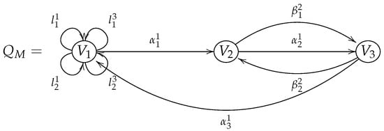
Figure 2. Brauer quiver induced by the Brauer configuration M.

The admissible ideal $I_{\Delta }$ is generated by the following relations (a and $a^{\prime }$ denote the first arrows of special cycles $C_{\alpha }$ associated with a vertex $\alpha$):

• $l_i^1{l}_j^3$, ${\left(l_i^1\right)}^2$, ${\left(l_i^3\right)}^2$, for all possible values of i and j.
• $l_i^3{\alpha }_1^1$, ${\alpha }_1^1{\beta }_1^2$, ${\beta }_1^2{\alpha }_3^1$, $C_1^1\alpha$, $C_2^1{\alpha }^{\prime }$, $C_1^1\sim C_2^1\sim C_3^2$, for all possible special cycles associated with Vertices 1, 2, and 3.

3. Main Results

This section provides Brauer configurations whose specializations give rise to left braces. Solutions of the YBE are obtained according to Lemma 1. The dimensions of the corresponding Brauer configuration algebras and their centers are also given.

3.1. Brauer Configurations of Type ${\mathfrak{F}}^{(i,j,k)}$

Let us define the following families of labeled (by the interval $[0,1]$) Brauer configurations, for which $i,k\ge 1$ are fixed and $1\le j\le 2^{i+1}$.

$${\mathfrak{F}}^{(i,j,k)}=({\mathfrak{F}}_0^{(i,j,k)},{\mathfrak{F}}_1^{(i,j,k)}=\{[f_{(i,j,k,0)},I_{(i,j,k,0)}],\dots ,[f_{(i,j,k,k)},I_{(i,j,k,k)}]\},{\nu }^{(i,j,k)},{\mathcal{O}}^{(i,j,k)}).$$

(25)

$${\mathfrak{F}}_0^{(i,j,k)}=\left\{\begin{array}{cc}\{a_{(i,j,k,0)},a_{(i,j,k,1)},a_{(i,j,k,2)}\},\hfill & \mathrm{if}i=k=1,\hfill \\ \{a_{(i,j,k,1)},a_{(i,j,k,2)}\},\hfill & \mathrm{if}i>1.\hfill \end{array}\right.$$

The words $w\left(f_{(i,j,k,h)}\right)$ associated with polygons $f_{(i,j,k,h)}$ are given by the following identities, for $0\le h\le k$.

$$w\left(f_{(i,j,k,h)}\right)=a_{(i,j,k,1)}^{k-h}{a}_{(i,j,k,2)}^h.$$

(26)

$${\nu }^{(i,j,k)}\left(a_{(i,j,k,h)}\right)=\left\{\begin{array}{cc}(1,2),\hfill & \mathrm{if}i=k=1,1\le j\le 4,h\in \{1,2\},\hfill \\ (t_k,1),\hfill & \mathrm{otherwise}.\hfill \end{array}\right.$$

Successor sequences $S_x$ associated with a given vertex $x\in {\mathfrak{F}}_0^{(i,j,k)}$ are built in such a way that, for $i,j$ and k fixed, it holds that

$$S_x=[f_{(i,j,k,0)},I_{(i,j,k,0)}]<[f_{(i,j,k,1)},I_{(i,j,k,1)}]<\dots <[f_{(i,j,k,k)},I_{(i,j,k,k)}].$$

(27)

$I_{(i,j,k,h)}$ denotes a subset of the interval $[0,1]\subset \mathbb{R}$, i.e., the Brauer configuration ${\mathfrak{F}}^{(i,j,k)}$ is labeled by the closed interval $[0,1]$.

Similarly, we define Brauer configurations ${\mathfrak{G}}^{(i,j,k)}$ such that

$${\mathfrak{G}}^{(i,j,k)}=({\mathfrak{G}}_0^{(i,j,k)},{\mathfrak{G}}_1^{(i,j,k)}=\{[g_{(i,j,k,0)},J_{(i,j,k,0)}],\dots ,[g_{(i,j,k,k)},J_{(i,j,k,k)}]\},{\nu }^{(i,j,k)},{\mathcal{O}}^{(i,j,k)}).$$

(28)

$${\mathfrak{G}}_0^{(i,j,k)}=\left\{\begin{array}{cc}\{b_{(i,j,k,0)},b_{(i,j,k,1)},b_{(i,j,k,2)}\},\hfill & \mathrm{if}i=k=1,\hfill \\ \{b_{(i,j,k,1)},b_{(i,j,k,2)}\},\hfill & \mathrm{if}i>1.\hfill \end{array}\right.$$

For $0\le h\le k$, it holds that

$$w\left(g_{(i,j,k,h)}\right)=b_{(i,j,k,2)}^h{b}_{(i,j,k,1)}^{k-h}.$$

(29)

Multiplicities and orientations are defined as for ${\mathfrak{F}}^{(i,j,k)}$.

As an example, we give the Brauer configuration algebra induced by the Brauer configuration ${\mathfrak{F}}^{(1,1,1)}$, for which:

$$\begin{array}{cc}\hfill {\mathfrak{F}}_0^{(1,1,1)}& =\{a_{(1,1,1,0)},a_{(1,1,1,1)},a_{(1,1,1,2)}\};{\mathfrak{F}}_1^{(1,1,1)}=\{[f_{(1,1,1,0)},I_{(1,1,1,0)},[f_{(1,1,1,1)},I_{(1,1,1,1)}]\},\hfill \\ \hfill w\left(f_{(1,1,1,0)}\right)& =a_{(1,1,1,0)}{a}_{(1,1,1,1)},w\left(f_{(1,1,1,1)}\right)=a_{(1,1,1,0)}{a}_{(1,1,1,2)},\hfill \\ \hfill \nu \left(a_{(1,1,1,0)}\right)& =(2,1),\nu \left(a_{(1,1,1,1)}\right)=\nu \left(a_{(1,1,1,2)}\right)=(1,2),\hfill \\ \hfill S_{a_{(1,1,1,0)}}& =[f_{(1,1,1,0)},I_{(1,1,1,0)}]<[f_{(1,1,1,1)},I_{(1,1,1,1)}],\hfill \\ \hfill S_{a_{(1,1,1,1)}}& =[f_{(1,1,1,0)},I_{(1,1,1,0)}],\hfill \\ \hfill S_{a_{(1,1,1,2)}}& =[f_{(1,1,1,1)},I_{(1,1,1,1)}].\hfill \end{array}$$

(30)

Figure 3 shows the Brauer quiver associated with the Brauer configuration ${\mathfrak{F}}^{(1,1,1)}$; for the sake of clarity, we assume the notation $a_{(i,j,k,h)}=h$, $f_{(i,j,k,h)}=f_h$ for vertices and polygons.

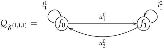
Figure 3. Brauer quiver induced by the Brauer configuration ${\mathfrak{F}}^{(1,1,1)}$.

The admissible ideal $I\subset \mathbb{F}{Q}_{{\mathfrak{F}}^{(1,1,1)}}$ is generated by relations of the following types:

• ${\left(l_1^j\right)}^3$;
• ${\alpha }_i^0{l}_i^j$, $l_i^j{\alpha }_i^0$, for all possible values of i and j;
• ${\alpha }_1^0{\alpha }_2^0{\alpha }_1^0$, ${\alpha }_2^0{\alpha }_1^0{\alpha }_2^0$.

According to identities (23) and (24), we have that for $1\le j\le 4$, it holds that

$$\begin{array}{cc}\hfill {\dim }_{\mathbb{F}}{\Lambda }_{{\mathfrak{F}}^{(1,j,1)}}& =4+2(2-1)+1(2-1)+1(2-1)=8,\hfill \\ \hfill {\dim }_{\mathbb{F}}Z\left({\Lambda }_{{\mathfrak{F}}^{(1,j,1)}}\right)& =1+5-3+2-2=3.\hfill \end{array}$$

(31)

The following Theorem 2 gives the properties of the Brauer configuration algebras ${\Lambda }_{{\mathfrak{F}}^{(i,j,k)}}$.

Theorem 2.

For $i,j,k\ge 1$ fixed and $1\le j\le 2^i+1$, the Brauer configuration algebra ${\Lambda }_{{\mathfrak{F}}^{(i,j,k)}}$ is indecomposable as an algebra and the Brauer configuration ${\mathfrak{F}}^{(i,j,k)}$ is reduced.

Proof. 

If $x\in {\mathfrak{F}}_0^{(i,j,k)}$, then

$${\nu }_x^{(i,j,k)}=\left\{\begin{array}{cc}{t}_k,\hfill & \mathrm{if}x\in \{a_{i,j,k,1},a_{i,j,k,2}\},\hfill \\ 2,\hfill & \mathrm{if}x=a_{(i,j,k,0)}.\hfill \end{array}\right.$$

Thus, ${\mathfrak{F}}^{(i,j,k)}$ has no truncated vertices.

Since:

• $a_{(1,j,1,0)}\in f_{(1,j,1,0)}\cap f_{(1,j,1,1)}$;
• $a_{(i,j,k,1)}\in f_{(i,j,k,0)}$;
• $a_{(i,j,k,2)}\in f_{(i,j,k,k)}$;
• $\{a_{i,j,k,1},a_{i,j,k,2}\}\subset {\displaystyle \bigcap _{h=1}^{k-1}}{f}_{(i,j,k,h)}$.

as multisets, then ${\mathfrak{F}}^{(i,j,k)}$ is connected. Thus, the result follows as a consequence of Theorem 1. We are done. □

As a consequence of Formulas (23) and (24), the following Corollary 1 gives formulas for the dimensions of an algebra of type ${\Lambda }_{{\mathfrak{F}}^{(i,j,k)}}$ and its center.

Corollary 1.

For $i\ge 1$, $k>1$, and $1\le j\le 2^{i+1}$ fixed, it holds that

$$\begin{array}{cc}\hfill {\dim }_{\mathbb{F}}{\Lambda }_{{\mathfrak{F}}^{(i,j,k)}}& =2(k+1)+4t_{(t_k-1)},\hfill \\ \hfill {\dim }_{\mathbb{F}}Z\left({\Lambda }_{{\mathfrak{F}}^{(i,j,k)}}\right)& =k+2.\hfill \end{array}$$

(32)

where $t_i=\frac{i(i+1)}{2}$ denotes the ith triangular number.

Proof. 

Note that, if $x\in {\mathfrak{F}}_0^{(i,j,k)}$, then $\nu \left(x\right)=(t_k,1)$. Furthermore, $|{\mathfrak{F}}_1^{(i,j,k)}|=k+1$. □

Corollary 2.

For $i\ge 1$, $\le j\le 2^{i+1}$, and $k\ge 1$ fixed, the algebra ${\Lambda }_{{\mathfrak{F}}^{(i,j,k)}}$ has a length grading induced from the path algebra $\mathbb{F}{Q}_{{\mathfrak{F}}^{(i,j,k)}}$, where $Q_{{\mathfrak{F}}^{(i,j,k)}}$ is the Brauer quiver associated with the Brauer configuration ${\mathfrak{F}}^{(i,j,k)}$.

Proof. 

For any $x\in {\mathfrak{F}}_0^{(i,j,k)}$, it holds that ${\nu }_x=t_k$. □

Remark 2.

Note that Theorem 3 and Corollaries 1 and 2 also hold for Brauer configuration algebras ${\Lambda }_{{\mathfrak{G}}^{(i,j,k)}}$ induced by Brauer configurations of type ${\mathfrak{G}}^{(i,j,k)}$.

3.2. Specializations

This section defines specializations $e_{(i,j,k)}\left({\mathfrak{F}}^{(i,j,k)}\right)$ of Brauer configurations by defining maps $e_{(i,j,k)}:{\mathfrak{F}}_0^{(i,j,k)}\to {[0,1]}^{[0,1]}$, where $i,k\ge 1$, $1\le j\le 2^{i+1}$ and ${[0,1]}^{[0,1]}$ is the set of functions from $[0,1]$ to $[0,1]$.

For $i\ge 1$, $1\le j\le 2^{i+1}$, and $k\ge 1$ fixed, we define $e_{(i,j,k)}\left({\mathfrak{F}}^{(i,j,k)}\right)$ in such a way that

$$\begin{array}{cc}\hfill e_{(i,j,1)}\left(a_{(i,j,1,0)}\right)\left(x\right)& =0,\mathrm{for}\mathrm{any}x\in [0,1],i\ge 1,1\le j\le 2^{i+1}.\hfill \end{array}$$

(33)

$$e_{(i,j,1)}\left(a_{(i,j,1,1)}\right)\left(x\right)=\left\{\begin{array}{cc}x,\hfill & \mathrm{if}x\in [0,\frac{2+3(j-1)}{2^{i+3}}],\hfill \\ \frac{1}{2}x+\frac{2+3(j-1)}{2^{i+4}},\hfill & \mathrm{if}x\in [\frac{2+3(j-1)}{2^{i+3}},\frac{2+3j}{2^{i+3}}-\frac{1}{2^{i+3}}],\hfill \\ 0,\hfill & \mathrm{if}x\in (\frac{2+3j}{2^{i+3}}-\frac{1}{2^{i+3}},1].\hfill \end{array}\right.$$

where $[0,\frac{2+3(j-1)}{2^{i+3}}]\cup [\frac{2+3(j-1)}{2^{i+3}},\frac{2+3j}{2^{i+3}}-\frac{1}{2^{i+3}}]$ corresponds to the label $I_{(i,j,1,0)}$ of $f_{(i,j,1,0)}$.

$$e_{(i,j,1)}\left(a_{(i,j,1,2)}\right)\left(x\right)=\left\{\begin{array}{cc}0,\hfill & \mathrm{if}x\in [0,\frac{2+3j}{2^{i+3}}-\frac{1}{2^{i+3}}),\hfill \\ 2x-\frac{2+3j}{2^{i+3}},\hfill & \mathrm{if}x\in [\frac{2+3j}{2^{i+3}}-\frac{1}{2^{i+3}},\frac{2+3j}{2^{i+3}}-\frac{1}{2^{i+4}}],\hfill \\ x,\hfill & \mathrm{if}x\in [\frac{2+3j}{2^{i+3}}-\frac{1}{2^{i+4}},1].\hfill \end{array}\right.$$

The label associated with $f_{(i,j,1,1)}$ is $I_{(i,j,1,1)}=[\frac{2+3j}{2^{i+3}}-\frac{1}{2^{i+3}},\frac{2+3j}{2^{i+3}}-\frac{1}{2^{i+4}}]\cup [\frac{2+3j}{2^{i+3}}-\frac{1}{2^{i+4}},1]$.

Remark 3.

If i and j are fixed, then we write $a_1^k\left(a_2^k\right)$ instead of $a_{(i,j,k,1)}$ ($a_{(i,j,k,2)}$). $a_1\left(x\right)=e_{(i,j,1)}\left(a_{(i,j,1,1)}\right)\left(x\right)$, $a_2\left(x\right)=e_{(i,j,1)}\left(a_{(i,j,1,2)}\right)\left(x\right)$, for any $x\in I_{i,j,1,0}$ ($x\in I_{(i,j,1,1)}$).

If $f\in {[0,1]}^{[0,1]}$ and $Supp\left(f\right)=\{x\in [0,1]\mid f(x)\ne 0\}$, then

$$\begin{array}{cc}\hfill Supp(a_1^k& =\underset{k-\mathrm{times}}{\underbrace{a_1\circ a_1\dots \circ a_1}})=[0,\frac{2+3(j-1)}{2^{i+3}}]\cup [\frac{2+3(j-1)}{2^{i+3}},\frac{2+3j}{2^{i+3}}-\frac{1}{2^{i+3}}],\hfill \\ \hfill Supp(a_1^{k-h}{a}_2^h& =\underset{(k-h)-\mathrm{times}}{\underbrace{a_1\circ a_1\dots \circ a_1}}\underset{h-\mathrm{times}}{\underbrace{a_2\circ a_2\dots \circ a_2}})=[\frac{2+3j}{2^{i+3}}-\frac{1}{2^{h+i+2}},\frac{2+3j}{2^{i+3}}-\frac{1}{2^{h+i+3}}],\hfill \\ \hfill Supp(a_2^k& =\underset{k-\mathrm{times}}{\underbrace{a_2\circ a_2\dots \circ a_2}})=I_{(i,j,k,k)},\hfill \\ \hfill I_{(i,j,k,k)}& =[\frac{2+3j}{2^{i+3}}-\frac{1}{2^{k+i+2}},\frac{2+3j}{2^{i+3}}-\frac{1}{2^{k+i+3}}]\cup [\frac{2+3j}{2^{i+3}}-\frac{1}{2^{k+i+3}},1].\hfill \end{array}$$

(34)

$a_1^{k-h}{a}_2^h$ is the specialization $e_{(i,j,k)}\left(f_{(i,j,k,h)}\right)$ of the word associated with the polygon $f_{(i,j,k,h)}$. It is a function of the form:

$$e_{(i,j,k)}\left(f_{(i,j,k,h)}\right)\left(x\right)=\left\{\begin{array}{cc}{a}_1^{k-h}{a}_2^h\left(x\right),\hfill & \mathrm{if}x\in [\frac{2+3j}{2^{i+3}}-\frac{1}{2^{h+i+2}},\frac{2+3j}{2^{i+3}}-\frac{1}{2^{h+i+3}}],\hfill \\ 0,\hfill & \mathrm{elsewhere}.\hfill \end{array}\right.$$

where $[\frac{2+3j}{2^{i+3}}-\frac{1}{2^{h+i+2}},\frac{2+3j}{2^{i+3}}-\frac{1}{2^{h+i+3}}]$ is the label $I_{(i,j,k,h)}$ associated with the polygon $f_{(i,j,k,h)}$.

The same notation is assumed for the Brauer configuration ${\mathfrak{G}}^{(i,j,k)}$. In such a case,

$$\begin{array}{cc}\hfill Supp(b_1^k& =\underset{k-\mathrm{times}}{\underbrace{b_1\circ b_1\dots \circ b_1}})=[0,\frac{2+3(j-1)}{2^{i+3}}]\cup [\frac{2+3(j-1)}{2^{i+3}},\frac{2+3j}{2^{i+3}}+\frac{1}{2^{i+j+2}}],\hfill \\ \hfill Supp(b_2^h{b}_1^{k-h}& =\underset{(k-h)-\mathrm{times}}{\underbrace{b_1\circ b_1\dots \circ b_1}}\underset{h-\mathrm{times}}{\underbrace{b_2\circ b_2\dots \circ b_2}})=I_{(i,j,k,h)},\hfill \\ \hfill Supp(b_2^k& =\underset{k-\mathrm{times}}{\underbrace{b_2\circ b_2\dots \circ b_2}})=[\frac{2+3j}{2^{i+3}}-\frac{1}{2^{k+i+2}},\frac{2+3j}{2^{i+3}}-\frac{1}{2^{k+i+3}}]\cup [\frac{2+3j}{2^{i+3}}-\frac{1}{2^{k+i+3}},1].\hfill \end{array}$$

(35)

$I_{(i,j,k,h)}=[\frac{2+3(j-1)}{2^{i+3}}+\frac{1}{2^{j-h+i+3}},\frac{2+3(j-1)}{2^{i+3}}+\frac{1}{2^{j-h+i+2}}]$ is the label associated with the polygon $g_{(i,j,k,h)}$.

$$e_{(i,j,1)}\left(b_{(i,j,1,1)}\right)\left(x\right)=\left\{\begin{array}{cc}x,\hfill & \mathrm{if}x\in [0,\frac{2+3(j-1)}{2^{i+3}}],\hfill \\ 2x-\frac{2+3(j-1)}{2^{i+5}},\hfill & \mathrm{if}[\frac{2+3(j-1)}{2^{i+3}},\frac{2+3j}{2^{i+3}}+\frac{1}{2^{i+j+2}}],\hfill \\ 0,\hfill & \mathrm{if}x\in (\frac{2+3j}{2^{i+3}}+\frac{1}{2^{i+j+2}},1].\hfill \end{array}\right.$$

$$e_{(i,j,1)}\left(b_{(i,j,1,2)}\right)\left(x\right)=\left\{\begin{array}{cc}0,\hfill & \mathrm{if}x\in [0,\frac{2+3j}{2^{i+3}}+\frac{1}{2^{i+j+2}}),\hfill \\ \frac{1}{2}x+\frac{2+3j}{2^{i+2}},\hfill & \mathrm{if}x\in [\frac{2+3j}{2^{i+3}}-\frac{1}{2^{i+3}},\frac{2+3j}{2^{i+3}}-\frac{1}{2^{i+4}}],\hfill \\ x,\hfill & \mathrm{if}x\in (\frac{2+3j}{2^{i+3}}-\frac{1}{2^{i+4}},1].\hfill \end{array}\right.$$

For $i,k\ge 1$ fixed, the specialized Brauer message ${\mathfrak{M}}^{e_{(i,j,k)}}\left({\mathfrak{F}}^{(i,j,k)}\right)$ has the form (see (20) and (21)):

$$\begin{array}{cc}\hfill {\mathfrak{M}}^{e_{(i,j,k)}}\left({\mathfrak{F}}^{(i,j,k)}\right)& =e_{(i,1,k)}\left(f_{(i,j,k,0)}\right)+e_{(i,2,k)}\left(f_{(i,j,k,1)}\right)+\dots +e_{(i,j,k,k)}\left(f_{(i,j,k,k)}\right)=F_{(i,j,k)},\hfill \\ \hfill F_{(i,j,k)}& =\underset{k-\mathrm{times}}{\underbrace{F_{(i,j,1)}\circ F_{(i,j,1)}\circ \dots \circ F_{(i,j,1)}}},\mathrm{for}1\le j\le 2^{i+1}fixed.\hfill \end{array}$$

(36)

For $i,k\ge 1$ fixed, we let ${\mathcal{M}}_{(i,j,k)}$ denote the set of specialized messages.

For $i,k\ge 1$, we define the sum of Brauer messages $F_{(i,j,k)},F_{(i,j^{\prime },k)}\in {\mathcal{M}}_{(i,j,k)}$ in such a way that

$$F_{(i,j,k)}+F_{(i,j^{\prime },k)}=F_{(i,j^{\prime },k)}\circ F_{(i,j,k)}.$$

(37)

Remark 4.

We adopt the same notation for Brauer messages and the corresponding operations associated with Brauer configurations of type ${\mathfrak{G}}^{(i,j,k)}$.

We let ${\mathfrak{H}}_{(i,j,k)}$ denote the subset of functions from $[0,1]$ to $[0,1]$ such that, for $i,k\ge 1$ fixed,

$$\begin{array}{cc}\hfill {\mathfrak{H}}_{(i,j,k)}& =\{f\in {[0,1]}^{[0,1]}\mid f=F_{(i,1,k)}^{{\alpha }_{1,1}}+G_{(i,1,k)}^{{\alpha }_{1,2}}+F_{(i,2,k)}^{{\alpha }_{2,1}}+G_{(i,2,k)}^{{\alpha }_{2,2}}+\dots \hfill \\ \hfill & \dots +F_{(i,2^{i+1},k)}^{{\alpha }_{2^{i+1,1}}}+G_{(i,2^{i+1},k)}^{{\alpha }_{2^{i+1,2}}},{\alpha }_{i,j}\ge 1\},\hfill \\ \hfill H_{(i,j,k)}^{{\alpha }_t}& =\underset{{\alpha }_t-\mathrm{times}}{\underbrace{H_{(i,j,k)}\circ H_{(i,j,k)}\circ \dots \circ H_{(i,j,k)}}},H\in \{F,G\}.\hfill \end{array}$$

(38)

It is worth recalling that Thompson’s group F (under composition) consists of those homomorphisms of the interval $[0,1]$, which satisfy the following conditions [26,27]:

• They are piecewise linear and orientation-preserving.
• In the pieces where the maps are linear, the slope is a power of 2.
• Points where slopes change their values are said to be breakpoints, which are dyadic, i.e., they belong to the set $B\times B$, where $B=[0,1]\cap \mathbb{Z}\left[\frac{1}{2}\right]$.

Breakpoints are used to identify any element $f\in F$ provided that such an element has finitely many breakpoints. In other words, if the set of pairs $\{[a_1,b_1],[a_2,b_2],\dots ,[a_k,b_k]\}$ represents f, it is assumed that $(a_0,b_0)=(0,0)\in f$, $(a_{k+1},b_{k+1})=(1,1)\in f$, and $\frac{b_{i+1}-b_i}{a_{i+1}-a_i}=2^s$, for some $s\ge 0$.

For instance, the set of pairs $\{(\frac{1}{8},\frac{1}{2}),(\frac{1}{4},\frac{3}{4}),(\frac{1}{2},\frac{7}{8})\}$ defines the function:

$$f\left(x\right)=\left\{\begin{array}{cc}4x,\hfill & \mathrm{if}x\in [0,\frac{1}{8}],\hfill \\ 2x+\frac{1}{4},\hfill & \mathrm{if}x\in [\frac{1}{8},\frac{1}{4}],\hfill \\ \frac{1}{8}(4x+5),\hfill & \mathrm{if}x\in [\frac{1}{4},\frac{1}{2}],\hfill \\ \frac{1}{4}(x+3),\hfill & \mathrm{if}x\in [\frac{1}{2},1].\hfill \end{array}\right.$$

Some of the main properties of Thompson’s group F is that it is torsion-free and contains a free abelian subgroup of infinite rank. Furthermore, F is an example of a torsion-free $F{P}_{\infty }$ group that is not of finite cohomological dimension.

Regarding Thompson’s group of type F, we have the following result.

Lemma 2.

For $i,k\ge 1$ fixed and $1\le j\le 2^i+1$, (${\mathfrak{H}}_{(i,j,k)},\circ )$ is a subgroup of the Thompson’s group F. In particular, ${\mathfrak{H}}_{(i,j,k)}$ is a subgroup of ${\mathfrak{H}}_{(i,j,k^{\prime })}$ if $k^{\prime }$ divides k.

Proof. 

Firstly, we note that, for any j, $1\le j\le 2^{i+1}$, the messages $F_{(i,j,k)}$ and $G_{(i,j,k)}$ are elements of F, provided that they are compositions of elements $F_{(i,j,1)}$ and $G_{(i,j,1)}$, which are elements of F by definition. In fact, $F_{(i,j,k)}$ and $G_{(i,j,k)}$ are defined as follows:

$$F_{(i,j,k)}\left(x\right)=\left\{\begin{array}{cc}x,\hfill & \mathrm{if}x\in [0,\frac{2+3(j-1)}{2^{i+3}}],\hfill \\ a_{(i,j,1,1)}^k,\hfill & \mathrm{if}x\in [\frac{2+3(j-1)}{2^{i+3}},\frac{2+3j}{2^{i+3}}-\frac{1}{2^{i+3}}],\hfill \\ a_{(i,j,1,1)}^{k-h}{a}_{(i,j,1,2)}^h,\hfill & \mathrm{if}x\in [\frac{2+3j}{2^{i+3}}-\frac{1}{2^{h+i+2}},\frac{2+3j}{2^{i+3}}-\frac{1}{2^{h+i+3}}],\hfill \\ a_{(i,j,1,2)}^k,\hfill & \mathrm{if}x\in [\frac{2+3j}{2^{i+3}}-\frac{1}{2^{k+i+2}},\frac{2+3j}{2^{i+3}}],\hfill \\ x,\hfill & \mathrm{if}x\in [\frac{2+3j}{2^{i+3}},1].\hfill \end{array}\right.$$

$$G_{(i,j,k)}\left(x\right)=\left\{\begin{array}{cc}x,\hfill & \mathrm{if}x\in [0,\frac{2+3(j-1)}{2^{i+3}}],\hfill \\ b_{(i,j,1,1)}^k,\hfill & \mathrm{if}x\in [\frac{2+3(j-1)}{2^{i+3}},\frac{2+3(j-1)}{2^{i+3}}+\frac{1}{2^{i+k+2}}],\hfill \\ b_{(i,j,1,2)}^h{b}_{(i,j,1,1)}^{k-h},\hfill & \mathrm{if}x\in [\frac{2+3(j-1)}{2^{i+3}}+\frac{1}{2^{i+k-h+3}},\frac{2+3(j-1)}{2^{i+3}}+\frac{1}{2^{i+k-h+2}}],\hfill \\ b_{(i,j,1,2)}^k,\hfill & \mathrm{if}x\in [\frac{2+3(j-1)}{2^{i+3}}+\frac{1}{2^{i+3}},\frac{2+3(j-1)}{2^{i+3}}+\frac{1}{2^{i+2}}],\hfill \\ x,\hfill & \mathrm{if}x\in [\frac{2+3(j-1)}{2^{i+3}}+\frac{1}{2^{i+2}},1].\hfill \end{array}\right.$$

where

$$\begin{array}{cc}\hfill a_{(i,j,1,1)}& =\frac{1}{2}x+\frac{2+3(j-1)}{2^{i+4}},a_{(i,j,1,2)}=2x-\frac{2+3j}{2^{i+3}},\hfill \\ \hfill b_{(i,j,1,1)}& =2x-\frac{2+3(j-1)}{2^{i+3}},b_{(i,j,1,2)}=\frac{1}{2}x+\frac{2+3j}{2^{i+4}}.\hfill \end{array}$$

(39)

Thus, for $i,j$ and k fixed, it holds that $G_{(i,j,k)}^m={\left(F_{(i,j,k)}^m\right)}^{-1}$. For

$f=F_{(i,1,k)}^{{\alpha }_{1,1}}+G_{(i,1,k)}^{{\alpha }_{1,2}}+F_{(i,2,k)}^{{\alpha }_{2,1}}+G_{(i,2,k)}^{{\alpha }_{2,2}}+\dots +F_{(i,2^{i+1},k)}^{{\alpha }_{2^{i+1,1}}}+G_{(i,2^{i+1},k)}^{{\alpha }_{2^{i+1,2}}}$

$g=F_{(i,1,k)}^{{\beta }_{1,1}}+G_{(i,1,k)}^{{\beta }_{1,2}}+F_{(i,2,k)}^{{\beta }_{2,1}}+G_{(i,2,k)}^{{\beta }_{2,2}}+\dots +F_{(i,2^{i+1},k)}^{{\beta }_{2^{i+1,1}}}+G_{(i,2^{i+1},k)}^{{\beta }_{2^{i+1,2}}}$, it holds that $f\circ g=F_{(i,1,k)}^{{\alpha }_{1,1}+{\beta }_{1,1}}+G_{(i,1,k)}^{{\alpha }_{1,2}+{\beta }_{1,2}}+F_{(i,2,k)}^{{\alpha }_{2,1}+{\beta }_{2,1}}+G_{(i,2,k)}^{{\alpha }_{2,2}+{\beta }_{2,2}}+\dots +F_{(i,2^{i+1},k)}^{{\alpha }_{2^{i+1,1}}+{\beta }_{2^{i+1},1}}+G_{(i,2^{i+1},k)}^{{\alpha }_{2^{i+1,2}}+{\beta }_{2^{i+1},2}}$.

Thus, $f\circ g\in F$. Therefore, ${\mathfrak{H}}_{(i,j,k)}$ is a subgroup of Thompson’s group. We are done. □

The following Theorem 3 proves that if the subgroup ${\mathfrak{H}}_{(i,j,k)}$ is endowed with the sum defined for messages ${\mathcal{M}}_{(i,j,k)}$, then it is a brace. Note that, if $f,g\in {\mathfrak{H}}_{(i,j,k)}$, then

$f=F_{(i,1,k)}^{{\alpha }_{1,1}}+G_{(i,1,k)}^{{\alpha }_{1,2}}+F_{(i,2,k)}^{{\alpha }_{2,1}}+G_{(i,2,k)}^{{\alpha }_{2,2}}+\dots +F_{(i,2^{i+1},k)}^{{\alpha }_{2^{i+1,1}}}+G_{(i,2^{i+1},k)}^{{\alpha }_{2^{i+1,2}}}$

$g=F_{(i,1,k)}^{{\beta }_{1,1}}+G_{(i,1,k)}^{{\beta }_{1,2}}+F_{(i,2,k)}^{{\beta }_{2,1}}+G_{(i,2,k)}^{{\beta }_{2,2}}+\dots +F_{(i,2^{i+1},k)}^{{\beta }_{2^{i+1,1}}}+G_{(i,2^{i+1},k)}^{{\beta }_{2^{i+1,2}}}$, and

$f+g=G_{(i,2^{i+1},k)}^{{\beta }_{2^{i+1,2}}}\circ F_{(i,2^{i+1},k)}^{{\beta }_{2^{i+1,1}}}\circ \dots \circ G_{(i,2,k)}^{{\beta }_{2,2}}\circ F_{(i,2,k)}^{{\beta }_{2,1}}$$\circ G_{(i,1,k)}^{{\beta }_{1,2}}\circ F_{(i,1,k)}^{{\beta }_{1,1}}\circ G_{(i,2^{i+1},k)}^{{\alpha }_{2^{i+1,2}}}\circ F_{(i,2^{i+1},k)}^{{\alpha }_{2^{i+1,1}}}\circ \dots \circ G_{(i,2,k)}^{{\alpha }_{2,2}}\circ F_{(i,2,k)}^{{\alpha }_{2,1}}\circ G_{(i,1,k)}^{{\alpha }_{1,2}}\circ F_{(i,1,k)}^{{\alpha }_{1,1}}\in {\mathfrak{H}}_{(i,j,k)}$.

Theorem 3.

For any $i,k\ge 1$ fixed and $1\le j\le 2^{i+1}$, it holds that $({\mathfrak{H}}_{(i,j,k)},\circ ,+)$ is a left brace.

Proof. 

Lemma 3 proves that $({\mathfrak{H}}_{(i,j,k)},\circ )$ is a group. In particular, $f+i{d}_{[0,1]}=f$, for any $f\in {\mathfrak{H}}_{(i,j,k)}$, i.e., $i{d}_{[0,1]}=0$. $f+(g+h)=(f+g)+h$, for any $f,g,h\in {\mathfrak{H}}_{(i,j,k)}$.

For $j\ne j^{\prime }$, let $D_{(i,(j,j^{\prime }),k)}^F$, $D_{(i,(j,j^{\prime }),k)}^G$, and $D_{(i,(j,j^{\prime }),k)}^{FG}$ be subsets of $[0,1]$ such that

$$\begin{array}{cc}\hfill D_{(i,(j,j^{\prime }),k)}^F& =\{x\in [0,1]\mid F_{(i,j,k)}\left(x\right)\ne x\}\cap \{x\in [0,1]\mid F_{(i,j^{\prime },k)}\left(x\right)\ne x\},\hfill \\ \hfill D_{(i,(j,j^{\prime }),k)}^G& =\{x\in [0,1]\mid G_{(i,j,k)}\left(x\right)\ne x\}\cap \{x\in [0,1]\mid G_{(i,j^{\prime },k)}\left(x\right)\ne x\},\hfill \\ \hfill D_{(i,(j,j^{\prime }),k)}^{FG}& =\{x\in [0,1]\mid F_{(i,j,k)}\left(x\right)\ne x\}\cap \{x\in [0,1]\mid G_{(i,j^{\prime },k)}\left(x\right)\ne x\}.\hfill \end{array}$$

(40)

Since $D_{(i,(j,j^{\prime }),k)}^F=D_{(i,(j,j^{\prime }),k)}^G=D_{(i,(j,j^{\prime }),k)}^{FG}=⌀$, it holds that

$$\begin{array}{cc}\hfill F_{(i,j,k)}\circ F_{(i,j^{\prime },k)}& =F_{(i,j^{\prime },k)}\circ F_{(i,j,k)},\hfill \\ \hfill G_{(i,j,k)}\circ G_{(i,j^{\prime },k)}& =G_{(i,j^{\prime },k)}\circ G_{(i,j,k)},\hfill \\ \hfill F_{(i,j,k)}\circ G_{(i,j^{\prime },k)}& =G_{(i,j^{\prime },k)}\circ F_{(i,j,k)},\hfill \\ \hfill F_{(i,j,k)}\circ G_{(i,j,k)}& =i{d}_{[0,1]},\hfill \\ \hfill G_{(i,j,k)}\circ F_{(i,j,k)}& =i{d}_{[0,1]}.\hfill \end{array}$$

(41)

Thus, for any $f,g\in {\mathfrak{H}}_{(i,j,k)}$, $f+g=g+f$. Moreover,

$$\begin{array}{cc}\hfill f\circ (g+h)+f& =f\circ f\circ h\circ g,\hfill \\ \hfill f\circ g+f\circ h& =f\circ h\circ f\circ g=f\circ f\circ h\circ g.\hfill \end{array}$$

(42)

We are done. □

The following elements of Thompson’s group F are examples of generators of the subgroup ${\mathfrak{H}}_{(1,j,1)}$.

$$F_{(1,1,1)}\left(x\right)=\left\{\begin{array}{cc}x,\hfill & \mathrm{if}x\in [0,\frac{1}{8}],\hfill \\ \frac{1}{2}x+\frac{1}{16},\hfill & \mathrm{if}x\in [\frac{1}{8},\frac{1}{4}],\hfill \\ 2x-\frac{5}{16},\hfill & \mathrm{if}x\in [\frac{1}{4},\frac{5}{16}],\hfill \\ x,\hfill & \mathrm{if}x\in [\frac{5}{16},1].\hfill \end{array}\right.$$

$$F_{(1,2,1)}\left(x\right)=\left\{\begin{array}{cc}x,\hfill & \mathrm{if}x\in [0,\frac{5}{16}],\hfill \\ \frac{1}{2}x+\frac{5}{32},\hfill & \mathrm{if}x\in [\frac{5}{16},\frac{7}{16}],\hfill \\ 2x-\frac{1}{2},\hfill & \mathrm{if}x\in [\frac{7}{16},\frac{1}{2}],\hfill \\ x,\hfill & \mathrm{if}x\in [\frac{1}{2},1].\hfill \end{array}\right.$$

$$F_{(1,3,1)}\left(x\right)=\left\{\begin{array}{cc}x,\hfill & \mathrm{if}x\in [0,\frac{1}{2}],\hfill \\ \frac{1}{2}x+\frac{1}{4},\hfill & \mathrm{if}x\in [\frac{1}{2},\frac{5}{8}],\hfill \\ 2x-\frac{11}{16},\hfill & \mathrm{if}x\in [\frac{5}{8},\frac{11}{16}],\hfill \\ x,\hfill & \mathrm{if}x\in [\frac{11}{16},1].\hfill \end{array}\right.$$

$$F_{(1,4,1)}\left(x\right)=\left\{\begin{array}{cc}x,\hfill & \mathrm{if}x\in [0,\frac{11}{16}],\hfill \\ \frac{1}{2}x+\frac{11}{32},\hfill & \mathrm{if}x\in [\frac{11}{16},\frac{13}{16}],\hfill \\ 2x-\frac{7}{8},\hfill & \mathrm{if}x\in [\frac{13}{16},\frac{7}{8}],\hfill \\ x,\hfill & \mathrm{if}x\in [\frac{7}{8},1].\hfill \end{array}\right.$$

$$G_{(1,1,1)}\left(x\right)=\left\{\begin{array}{cc}x,\hfill & \mathrm{if}x\in [0,\frac{1}{8}],\hfill \\ 2x-\frac{1}{8},\hfill & \mathrm{if}x\in [\frac{1}{8},\frac{3}{16}],\hfill \\ \frac{1}{2}x+\frac{5}{32},\hfill & \mathrm{if}x\in [\frac{3}{16},\frac{1}{4}],\hfill \\ x,\hfill & \mathrm{if}x\in [\frac{1}{4},1].\hfill \end{array}\right.$$

$$G_{(1,2,1)}\left(x\right)=\left\{\begin{array}{cc}x,\hfill & \mathrm{if}x\in [0,\frac{5}{16}],\hfill \\ 2x-\frac{5}{16},\hfill & \mathrm{if}x\in [\frac{5}{16},\frac{3}{8}],\hfill \\ \frac{1}{2}x+\frac{1}{4},\hfill & \mathrm{if}x\in [\frac{3}{8},\frac{7}{16}],\hfill \\ x,\hfill & \mathrm{if}x\in [\frac{7}{16},1].\hfill \end{array}\right.$$

$$G_{(1,3,1)}\left(x\right)=\left\{\begin{array}{cc}x,\hfill & \mathrm{if}x\in [0,\frac{1}{2}],\hfill \\ 2x-\frac{1}{2},\hfill & \mathrm{if}x\in [\frac{1}{2},\frac{9}{16}],\hfill \\ \frac{1}{2}x+\frac{11}{32},\hfill & \mathrm{if}x\in [\frac{9}{16},\frac{5}{8}],\hfill \\ x,\hfill & \mathrm{if}x\in [\frac{5}{8},1].\hfill \end{array}\right.$$

$$G_{(1,4,1)}\left(x\right)=\left\{\begin{array}{cc}x,\hfill & \mathrm{if}x\in [0,\frac{11}{16}],\hfill \\ 2x-\frac{11}{16},\hfill & \mathrm{if}x\in [\frac{11}{16},\frac{3}{4}],\hfill \\ \frac{1}{2}x+\frac{7}{16},\hfill & \mathrm{if}x\in [\frac{3}{4},\frac{13}{16}],\hfill \\ x,\hfill & \mathrm{if}x\in [\frac{13}{16},1].\hfill \end{array}\right.$$

4. Concluding Remarks

We defined Brauer configurations of type ${\mathfrak{F}}^{(i,j,k)}$, which induce reduced and indecomposable Brauer configuration algebras. Specializations of the corresponding Brauer messages give rise to braces associated with Thompson’s group F. Such braces allow building non-degenerate involutive set-theoretical solutions of the YBE.

Future Work

The following are interesting tasks to carry out in the future:

• To determine braces of type ${\mathfrak{H}}_{(i,j,k)}$ associated with Thompson’s groups of type T and V.
• To determine braces based on the Cayley graph of Thompson’s group, $F,T$, and V.
• To give applications of the obtained results in graph energy theory, cryptography, and coding theory.

References

- Yang, C.N. Some exact results for the many-body problem in one dimension with repulsive delta-function interaction. Phys. Rev. Lett. 1967, 19, 1312–1315. [Google Scholar] [CrossRef]
- Baxter, R.J. Partition function for the eight-vertex lattice model. Ann. Phys. 1972, 70, 193–228. [Google Scholar] [CrossRef]
- Caudrelier, V.; Crampé, N. Exact results for the one-dimensional many-body problem with contact interaction: Including a tunable impurity. Rev. Math. Phys. 2007, 19, 349–370. [Google Scholar] [CrossRef]
- Cedó, F.; Jespers, E.; Oniński, J. Braces and the Yang–Baxter equation. Commun. Math. Phys. 2014, 327, 101–116. [Google Scholar] [CrossRef]
- Nichita, F.F. Introduction to the Yang–Baxter equation with open problems. Axioms 2012, 1, 33–37. [Google Scholar] [CrossRef]
- Nichita, F.F. Yang–Baxter equations, computational methods and applications. Axioms 2015, 4, 423–435. [Google Scholar] [CrossRef]
- Massuyeau, G.; Nichita, F.F. Yang–Baxter operators arising from algebra structures and the Alexander polynomial of knots. Comm. Algebra 2005, 33, 2375–2385. [Google Scholar] [CrossRef]
- Kauffman, L.H.; Lomonaco, S.J. Braiding operators are universal quantum gates. New J. Phys. 2004, 6, 134. [Google Scholar] [CrossRef]
- Turaev, V. The Yang–Baxter equation and invariants of links. Invent. Math. 1988, 92, 527–533. [Google Scholar] [CrossRef]
- Rump, W. Modules over braces. Algebra Discret. Math. 2006, 2, 127–137. [Google Scholar]
- Rump, W. Braces, radical rings, and the quantum Yang–Baxter equation. J. Algebra 2007, 307, 153–170. [Google Scholar] [CrossRef]
- Ballester-Bolinches, A.; Esteban-Romero, R.; Fuster-Corral, N.; Meng, H. The structure group and the permutation group of a set-theoretical solution of the quantum Yang–Baxter equation. Mediterr. J. Math. 2021, 18, 1347–1364. [Google Scholar] [CrossRef]
- Green, E.L.; Schroll, S. Brauer configuration algebras: A generalization of Brauer graph algebras. Bull. Sci. Math. 2017, 121, 539–572. [Google Scholar] [CrossRef]
- Cañadas, A.M.; Gaviria, I.D.M.; Vega, J.D.C. Relationships between the Chicken McNugget Problem, Mutations of Brauer Configuration Algebras and the Advanced Encryption Standard. Mathematics 2021, 9, 1937. [Google Scholar] [CrossRef]
- Moreno Cañadas, A.; Rios, G.B.; Serna, R.J. Snake graphs arising from groves with an application in coding theory. Computation 2022, 10, 124. [Google Scholar] [CrossRef]
- Agudelo, N.; Cañadas, A.M.; Espinosa, P.F.F. Brauer configuration algebras defined by snake graphs and Kronecker modules. Electron. Res. Arch. 2022, 30, 3087–3110. [Google Scholar]
- Espinosa, P.F.F. Categorification of Some Integer Sequences and Its Applications. Ph.D. Thesis, Universidad Nacional de Colombia, Bogotá, Colombia, 2021. [Google Scholar]
- Drinfeld, V.G. On unsolved problems in quantum group theory. Lect. Notes Math. 1992, 1510, 1–8. [Google Scholar]
- Etingof, P.; Schedler, T.; Soloviev, A. Set-theoretical solutions to the quantum Yang–Baxter equation. Duke Math. J. 1999, 100, 169–209. [Google Scholar] [CrossRef]
- Gateva-Ivanova, T.; Van den Bergh, M. Semigroups of I-type. J. Algebra 1998, 308, 97–112. [Google Scholar] [CrossRef]
- Guarnieri, L.; Vendramin, L. Skew braces and the Yang–Baxter equation. Math. Comput. 2017, 85, 2519–2534. [Google Scholar] [CrossRef]
- Andrews, G.E. The Theory of Partitions; Cambridge University Press: Cambridge, UK, 2010. [Google Scholar] [CrossRef]
- da Fontoura Costa, L. Multisets. arXiv 2021, arXiv:2110.12902. [Google Scholar]
- Schroll, S. Brauer Graph Algebras. In Homological Methods, Representation Theory, and Cluster Algebras, CRM Short Courses; Assem, I., Trepode, S., Eds.; Springer: Cham, Switzerland, 2018; pp. 177–223. [Google Scholar]
- Sierra, A. The dimension of the center of a Brauer configuration algebra. J. Algebra 2018, 510, 289–318. [Google Scholar] [CrossRef]
- Belk, J.M. Thompson’s group F. Ph.D. Thesis, Cornell University, Ithaca, NY, USA, 2004. [Google Scholar]
- Burillo, J.; Cleary, S.; Stein, M.; Taback, J. Combinatorial and Metric Properties of Thompson’s Group T. Trans. Amer. Math. Soc. 2009, 361, 631–652. [Google Scholar] [CrossRef]
Disclaimer/Publisher’s Note: The statements, opinions and data contained in all publications are solely those of the individual author(s) and contributor(s) and not of MDPI and/or the editor(s). MDPI and/or the editor(s) disclaim responsibility for any injury to people or property resulting from any ideas, methods, instructions or products referred to in the content. |
© 2022 by the authors. Licensee MDPI, Basel, Switzerland. This article is an open access article distributed under the terms and conditions of the Creative Commons Attribution (CC BY) license (https://creativecommons.org/licenses/by/4.0/).