1. Introduction
A growing number of applications, such as spatial distribution mapping, dynamic sensors coverage, and environmental extensive area monitoring, have motivated the development of both sensing hardware and algorithms for target-oriented mobile sensor networks [
1,
2]. Any such application requires ad hoc customization of hardware and software solutions. Large area monitoring, for example, presents the main problem for biasing certain regions of interest. Indeed, some parts might be prioritized based on prior knowledge and due to an inherent time-constraint that prohibits an exhaustive search of the area; for instance, in the case of emergencies and search and rescue operations. This situation is met during the oil spill monitoring of large marine regions, and in general, in all pollution events involving diffusion [
3]. The most probable scenario is that areas in which human beings, pollution activities, or hazardous materials are likely to be present should be searched first, while regions with less probability of containing these features are searched later. Consequently, both inferential statistical methods and mobile sensor networks able to navigate from an initial configuration within a region containing shaped obstacles were developed [
4]. In this paper, we focus the attention on coordination algorithms to improve the capability of mobile sensors networks in covering and monitoring relevant portions of larger areas. Our proposed solution to this problem is obtained using centroidal Voronoi partitions.
The centroidal Voronoi partition is a widely used scheme of portioning a given space, and finds applications in many fields, such as image processing, sensor coverage, crystallography, and CAD [
5,
6,
7,
8]. The basic components of a Voronoi partition are:
- (i)
A space, which is to be partitioned;
- (ii)
A set of sites, or nodes or generators;
- (iii)
A distance measure, such as the Euclidean distance.
In the case of homogeneous sensors with a typical circular sensing area, the sensor located in a Voronoi cell V
i is closest to all the points q ∈ V
i, and hence, by the strictly decreasing variation of sensors effectiveness with distance, the sensor is most effective within V
i, provided the circular area covered by the sensor does not cover the entire cell. Thus, the Voronoi decomposition leads to optimal partitioning of the space, in the sense that each sensor is most effective within its corresponding Voronoi cell. In the heterogeneous case too, it is easy to see that each sensor is most effective in its own generalized Voronoi cell. Since the partitioning is optimal, it is necessary to find the location of each sensor within its generalized Voronoi cell. Voronoi-based approaches have been used in the recent past for optimizing the coverage of mobile sensor networks. For instance, in [
9], the Maxmin-vertex and Maxmin-edge algorithms are proposed to maximize the minimum distance of every sensor form the vertices and edges respectively of its Voronoi cells. In [
10], such results are improved by also taking into consideration the adaptive ranges of sensors based on their respective residual energy. In [
11], the authors proposed to consider a heterogeneous network made of both static and mobile sensors, and a bidding protocol for the placement of the mobile ones is proposed. Intuitively, mobile sensors are treated as servers to heal possible coverage holes left by the network as a whole. In this framework, optimization is also achieved through the distributed calculation of the Voronoi partition. With respect to these previous works that have shown the powerfulness of the Voronoi-based approaches in coverage improvement, in this paper, a further element is considered which is of relevance when dealing with environmental monitoring; i.e., adaptive prioritizing of areas to be monitored.
In the specific case of marine monitoring, adaptability is necessary to deal with (i) changing conditions in maritime traffic, weather and currents, and (ii) available knowledge of pollution events that have already taken place. This variable information should be put in relation to the variable impacts that events can have on different areas; e.g., due to the existence of marine parks, the presence of endangered animal species and proximity to shores.
Indeed, spills of oil and related petroleum products in marine environments can have a severe biological and economic impact [
12,
13]. With modern remote sensing instrumentation, such pollution events can be monitored on the open ocean around the clock. The monitoring of large marine areas generally involves complex marine information systems [
14], which act as catalysts to integrate data from multiple and disparate data sources. Each source provides a specific piece of information, and through a suitable fusion and correlation process, they offer as a whole, a comprehensive characterization of the status of a marine area in terms of pollution events, maritime traffic, weather, and oceanic currents. In this process, key sources are SAR and optical satellite imaging to discover and quantify both oil slicks and real vessel traffic; the Automatic Identification System (AIS) for real-time identification and trajectory analysis of vessels passing through an area; and airborne hyperspectral sensors for detection and precise characterization of oil spills.
Sensorized buoys and surface and underwater vehicles can also be used to enforce remote monitoring. Indeed, autonomous underwater vehicles (AUVs) and mobile buoys equipped with different sensor devices are excellent candidates for real-time monitoring of oil spills through areas where the pollution events can take place. A new generation of buoys dedicated to oil spill monitoring is becoming available in a prototypal shape [
15] or in their commercial evolution. Other interesting sources of information are based on crowd-sensing methodologies [
16].
Environmental decision support systems (EDSS) are employed to orchestrate and make optimal and sustainable use of available monitoring and interventional resources. According to the survey [
17], routine goals are (i) to actuate policies for confirming partial observations obtained by one source by collecting further information and (ii) to prioritize monitoring according to an adaptive risk map. For instance, if a slick is detected by remote sensing, in situ sensors such as buoys or AUVs can be deployed to assess its presence. Additionally, marine currents and weather conditions can increase the impact and the area affected by the possible pollution events.
The results presented in this paper were obtained having in mind (but are not limited to) the monitoring of large marine areas where oil spill events can take place, and where the diffusion evolution of any oil slick is known a priori. In addition, we consider marine sensors equipped with sensing hardware to consist mainly of an electronic nose, a bathymetric sensor, a GPS device, an anemometer, a motor for self-dislocation depending on a pollution event, and a complete communication set up with a remote station.
Actually, our simulation considers minor influences of weather and low marine waves, and low velocity for pollution event drift, so that the diffusion dynamics can be considered slow with respect to the sensor network’s self-dislocation, which can be considered fast. The pollution events have been considered uncorrelated and were simulated with a Poisson distribution. Similar results were obtained with non-Poisson distributions.
The results show the capacity and the limits of event-dependent real-time monitoring of a sensor network. One of the limiting aspects is due to the real hardware facilities, especially for what regards real-time communication between the sensors and a remote station. The communication set up as considered in this paper is rather idealized; nevertheless, it is in line with the recent communication capabilities that will be available on sensorized devices for real-time monitoring of large marine areas.
The paper is organized as follows. In
Section 2, we introduce the modeling of pollution events using a Poisson distribution and describe the Voronoi tessellation arising from a number of geolocalized events. In
Section 3, details about Voronoi partitions, both classical and generalized, are given. In
Section 4, we introduce an objective function to be maximized for optimal monitoring of an area subject to a static risk of pollution events. In this scenario, mobile sensors should follow a certain physical velocity field to move from their initial configurations to the optimal one. In
Section 5, we assume that the risk of pollution changes over time in response to external events, diffusion and weathering; in this scenario, an iterative algorithm is proposed for letting the sensor network dislocate itself in an optimal way. Further, experimental simulations are described. Finally, in
Section 6 we derive our conclusions.
The main contributions of the paper can be summarized as follows:
- -
A solution for the optimal displacement of a sensor network is proposed for the monitoring of large areas. The solution is based on formalized geometrical methods using Voronoi centroidal tessellation.
- -
The proposed solution is fitted into an iterative algorithm, which can evolve in real-time and continuously, the displacement of the network in response to dynamic events and changes in risk.
- -
The results are proven theoretically and with numerical simulations.
2. Modeling of Pollution Events
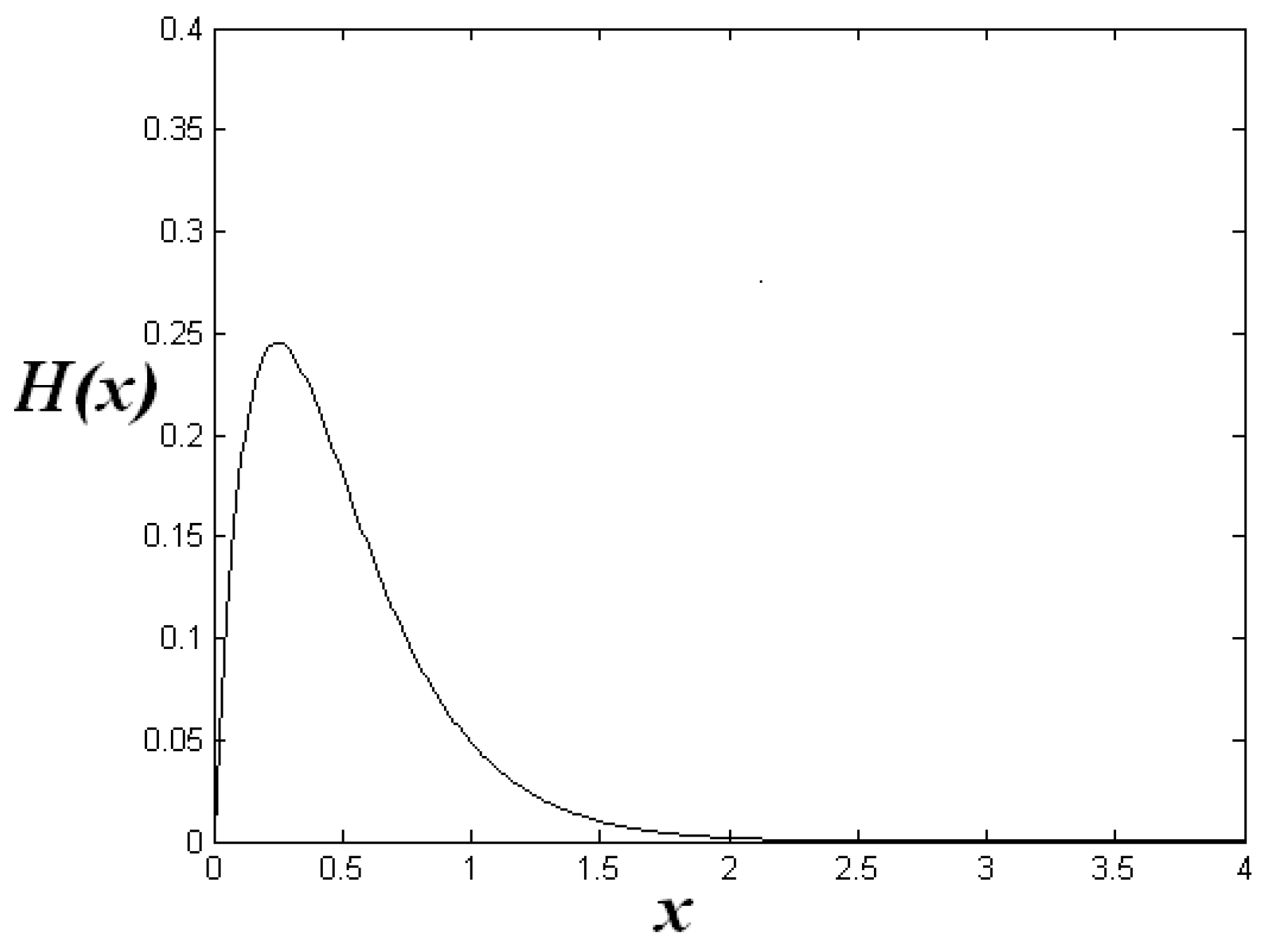
The first approach for monitoring a large area is given by the regular and symmetric dislocation of the sensors. Nevertheless, this approach is not practicable if the number of sensors with a finite radius of sensing power is not enough to cover the large area to be monitored. In addition, we have to consider the dislocation as event-dependent; i.e., considering the possible pollution source. An unwanted event is a random variable. Therefore, the immediate suggestion for a suitable event-dependent dislocation of a number of sensor networks is given by the Voronoi tessellations. A great number of natural phenomena are described by Voronoi tessellations; in this section, we try to respond to the main question: why should the optimal dislocations in a large area of a network composed by sensors with circular sensing power follow a centroidal Voronoi tessellation? To give an answer to this question, the starting point is to introduce the probability density function (PDF) for the occurrence of a pollution event, x. The reasonable shape of a PDF for a stochastic event is a Poisson distribution:
where λ is the hazard rate of the exponential distribution. Let us consider the sum of two uncorrelated events, y, the variable change, y = 2x, and x = 1/λ. The PDF (Equation (1)) can be written as:
The result in Equation (2) can be written using a gamma variate distribution [
18,
19] as a function of the space dimension d; in our case d = 2.
where, now, 0 ≤ x < ∞, and Γ(2d) is the gamma function with argument 2d. That PDF (Equation (3)) has a mean of μ = 1 and variance σ
2 = 1/d. The gamma PDF can be generalized by introducing new additional parameters that take into account the complexity of the real situation, pollution sources, environmental weather, etc. In this paper, we restrict ourselves to gamma PDF as in Equation (3).
Figure 1 shows the distribution as given by Equation (3) of pair events distance; i.e., the distance between two events close one each other.
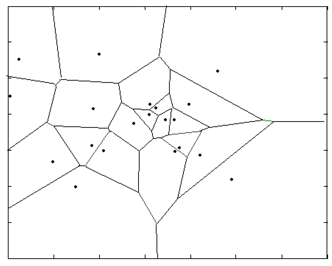
Let us consider n pollution events, distributed randomly in a square area. The monitoring of such diffusion processes can be made considering the equivalent Voronoi diagram, where the vertexes are coincident with the pollution events coordinates (see
Figure 2). Similar results are obtained when the events are located using a Gaussian distribution. This is the case of pollution events with a correlation, anywhere the result does not present a significant difference.
3. Basic Properties for a Voronoi Partition
A standard Voronoi partition can be introduced as follows: A collection {W
i}, i ∈ {1,2,…,N} of subsets of a space X with disjoint interiors is said to be a partition of X if ∪
iW
i = X. Let Q ⊂ ℜ
d be a convex polytope in d-dimensional Euclidean space. Let P = {p
1, p
2, …, p
N}, p
i ∈ Q be the set of nodes of generators in Q. The Voronoi partition generated by P with respect to the Euclidean norm is the collection {V
i(P)}, i ∈ {1, 2, …, N}, and is defined as:
where ‖ ⋅ ‖ denotes the Euclidean norm. The Voronoi cell V
i is the collection of those points that are closest (with respect to the Euclidean metric) to p
i compared to any other point in P. In ℜ
2, the boundary of each bounded Voronoi cell is the union of a finite number of line segments forming a closed °C curve. For example, the intersection of any two Voronoi cells can be null, a line segment, or a point. In d-dimensional space, the boundaries of the Voronoi cells are unions of convex subsets of at most d-1 dimensional hyperplanes in ℜ
d, and the intersection of two Voronoi cells can be a convex subset of a hyperplane or a null set. Each of the Voronoi cells is a topologically connected non-null set. Generalizations of the above Voronoi basic partition to suit specific applications can be found in the literature [
12,
13]. A possible generalization of the Voronoi partition can be introduced considering a space Q ⊂ ℜ
d, sand et of points called nodes or generators P = {p
1, p
2, …, p
N}, p
i ∈ Q, with p
i ≠ p
j, whenever i ≠ j, and monotonically decreasing analytic functions f
i: ℜ + → ℜ, where f
i is called a node function for the i-th node. It is possible to define a collection {V
i}, i ∈ {1, 2,…,N}, with mutually disjoint interiors, such that Q = ∪
iV
i, where V
i is now defined as:
We call {Vi}, i ∈ {1, 2, …, N} a generalized Voronoi partition of Q with nodes P and node functions fi. In this application, it should be noted that Vi can be topologically non-connected and may contain Voronoi cells. In addition, it should be noted that q ∈ Vi means that the i-th sensor is the most effective in sensing at point q. In a standard Voronoi partition used in a homogeneous case, the ≤ sign for distances ensures that i-th sensor is most effective in Vi. Finally, the condition that fi is analytic implies that for every i, j ∈ {1, 2,…, N}, fi-fj is analytic. By the properties of a real analytic function, it derives that the set of intersection points between any two-node functions is a set of measure zero. This ensures that the intersection of any two cells is a set of measure zero; that is, the boundary of a cell is a set is made up of the union of at most d-1 dimensional subsets of ℜd; otherwise, the requirements that the cells should have mutually disjoint interiors may be violated. The analyticity of the node functions {fi} is a sufficient condition to avoid this possibility.
4. Optimization in the Localization of Event-Dependent Mobile Sensors Network
In this Section, a solution to optimal monitoring of an area by means of mobile sensors with limited radial sensing ranges is proposed. Such sensors can either be mounted on buoys with motion capabilities or full-fledged AUVs or unmanned surface vehicles (USVs). As stated in the introduction, it is assumed that sensors can navigate quite fast with respect to the evolution of a pollution event by diffusion, marine currents, and weathering.
Let us consider a large area to be monitored by N sensors; the cost of real-time monitoring is rather high. Unwanted events to be monitored trigger a sensor network to navigate from an initial configuration towards a specific region within the large area where the probability of encountering unwanted events is higher.
Let Q ⊂ ℜ
d be a convex polytope, the space in which the sensors have to be deployed, and V
i ⊂ Q be the generalized Voronoi cell corresponding to the i-th node; we introduce a continuous density distribution function φ: Q → [0,1], where the density φ(q) is the probability of an event of interest occurring in q ∈ Q, and P = {p
1, p
2, …, p
N}, p
i ∈ Q is the configuration of N sensors [
20].
It is well known that the generalized Voronoi decomposition splits the objective function into a sum of contributions from each generalized Voronoi cell. As a consequence, the optimization problem can be solved in a spatially distributed manner; i.e., each sensor solving the part of objective function corresponding to its cell using only local information can achieve the optimal configuration.
Besides, another essential characteristic of the sensor network, as considered in this paper, is that any sensor possesses a limited range of action; with the sensing capability that decreases as a logarithm of the distance from the centroid. This limitation must be taken in due consideration. Let Ri be the limit on the range of the sensors and f (pi, Ri) be a closed disk centered at pi with a radius Ri. The i-th sensor has access to information only from points in the set Vi ∩ f (pi, Ri).
Let us consider the following objective function to be maximized:
where || . || is the Euclidean distance and f
i = 0 if ||q-p
i|| > R
i. It is possible to define the derivative of H (P) as follows.
In addition, it is possible to introduce the critical points defined as the points mass and the centroid of the V
i cells.
where
is the set of centroids where the mobile sensors must be dislocated, defined later. The centroids set has the property
∈Q because Q is an invariant set for Equation (8), while on the contrary, it is not guaranteed that
∈V
i. The dynamical properties of the mobile sensors network to be dislocated in an optimal configuration make it possible to write the basic control law as
where the single mobile sensor moves toward
for k > 0. Using the properties of the gradient with respect to p
i as in Equation (8), we can write
One main problem for the optimal dislocation of the mobile sensors is the convergence to the ideal centroid locations when a pollution event must be monitored. In this case, the uncovered area could generate more difficulties in producing a real convergence, but this problem can be dropped using effective k parameters in Equation (9). The problem of an effective convergence of a common radius sensor network that is unable to cover a large area is very close to that of the class of heterogeneous sensor networks [
20]. In our case, the effective k parameter implies that the mobile sensors have higher dislocating speed with respect to the evolution velocity of a pollution event. The pollution event, for example, an oil spill, modifies its shape on the marine surface due to weather conditions: if the event time-scale, τ, is τ < <1/k, then it is reasonable to expect a fast convergence to the optimal centroids. The control law, Equation (9), drives the sensors towards their optimal configurations that correspond to the arrangement that guarantees the maximum sensing power at the lowest cost. This is because the closed-loop system for the sensors networks is modeled using a first-order dynamical system that is globally asymptotically stable for an effective choice of k parameters; this is translated in the time property of H (P), which we supposed to be continuous.
The Equation (11) assures that the initial configurations of localized sensors converge to the optimal centroids .
One special problem is the ability of the sensors network to relocate themselves as a function of a pollution event (for example, an oil spill) whose shape changes in time due to diffusion and weathering. If the velocity of the sensor network is faster than the characteristic oil slick time diffusion, the sensing power of the sensors network is hugely enforced. Suppose a diffusion process evolves in the convex polytope space Q: Q ∈ ℜ2, where ρ (x, y): Q → ℜ+ can be used to represent the pollutant concentration over Q, where the dynamic process is modeled by a partial differential equation (PDE). The possibility to reorganize the sensors, relocating them to enforce their sensing power, is generally energy consuming; for this reason, the control law for the converge of the sensors toward their final centroids location must be constrained to the sensing power, which in this work we consider as Esensing (ri) = a⋅ri, for ri < Ri and Esensing (ri) = 0 otherwise, where a is constant and i is referred to the i-th sensor.
If the pollution event velocity in a given direction is v
event; then the control law (9) must be written as
where α = v
sensor/v
event is a parameter denoting how much faster the mobile sensor must be with respect to pollution velocity v
event; μ is a positive defined value taking into account the distance from the centroids to which converge. The control law (Equation (12)) makes the sensors move toward their respective centroids with a constant speed v
sensor when they are at a distance further than μ from the corresponding centroids and slow down as they approach them. The control law (Equation (12)) is calculated at regular steps using new centroids
as a function of the event. Suppose that at time t = 0, a pollution event is located at x0, y0: the initial shape ρ0 is a point. Under the effects of environmental parameters, ρ changes with time, and then at regular time steps, the centroids set is recalculated and the re-dislocation of mobile sensors occurs, consequently, until the highest sensing activity is made when two centroids set are coincident during two subsequent time steps checks.
Let us consider now, the possibility of a dislocation of the sensors network from an initial set of centroids to a new set of centroids when an unwanted event must be taken into consideration. When the time evolution of pollutant concentration ρ (x, y, t) is known, it is possible to calculate masses and centroids on region V
i at regular time steps as
The masses and centroids are recalculated using a sampling time, generally a fraction of α using an algorithm very close to Lloyd Centroidal algorithm [
21,
22,
23,
24] applied to sensors with a limited sensing radius, as in
Figure 3. When possible, the dynamical changes of ρ(|q-p
i|,t) are usually modeled by a partial differential equation [
13]. Because in many real situations the shape of ρ(|q-p
i|,t) is unknown, we advance the idea that ρ(|q-p
i|,t) could be substituted by a Poisson distribution of random events, so that ρ(|q-p
i|,t) can occur in one point, as described by
Figure 2, and evolve with low dynamics. In this manner, the n sensors can dislocate themselves to develop higher sensing power, thereby neutralizing the pollution as quickly as possible without making the area of interest overdosed.
5. Numerical Results and Discussion
Our method is based on the assumption that the occurrence of a random pollution event is an element of a more general class of events that follows a Poisson distribution, as described in
Figure 1,
Figure 2 and
Figure 3. The sensors’ capability can be considered more effective if they can be located in a general configuration, where the pollution event occupies one site, and the sensors the other ones.
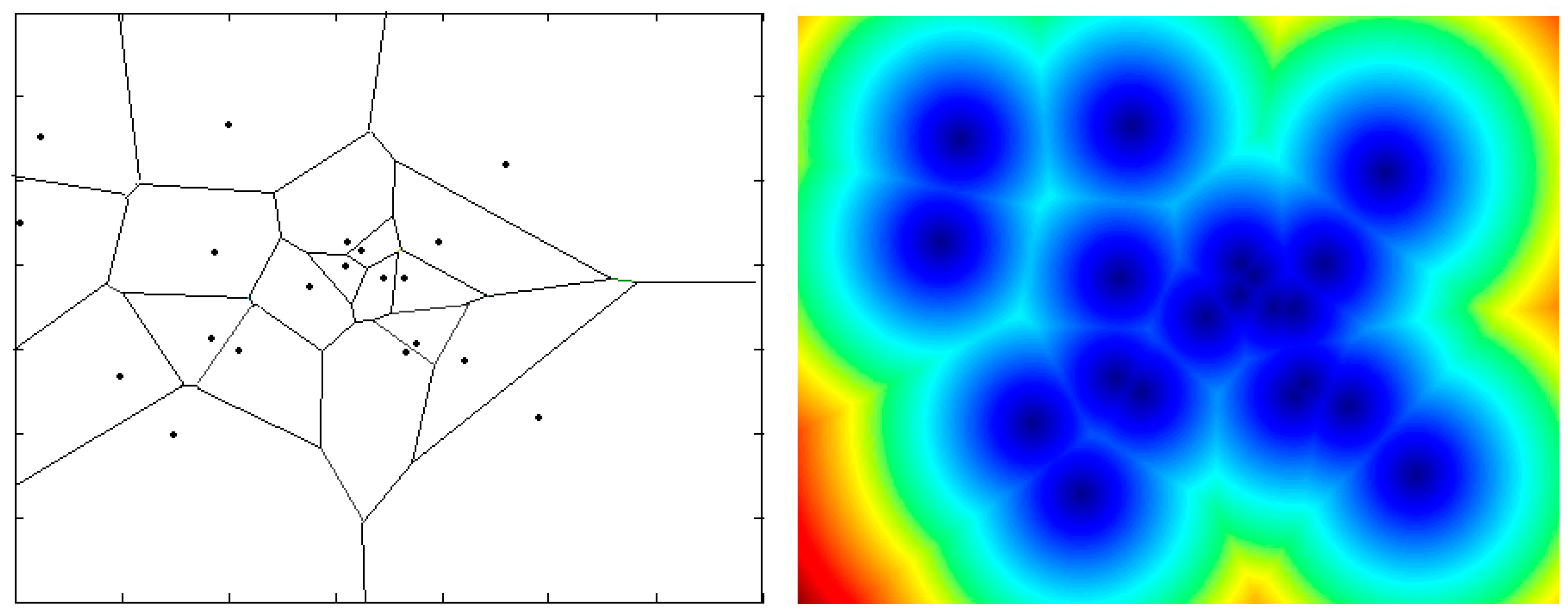
Figure 3 represents both the Voronoi diagram and the corresponding power sensing using sensors with limited sensing radii. As the pollution event, described by ρ(|q-p
i|,t), changes due to environmental conditions, the sensors must be re-dislocated on the positions coinciding with the centroids calculated using Equation (13). Because the shape of ρ(|q-p
i|,t) is generally unknown, we can hypothesize that at regular time steps, the new location of ρ(|q-p
i|,t) is on a position still described by the same Poisson distribution, that in our model represents a primitive partitions of space, which the Voronoi diagram represents the most effective operability of the sensors networks (
Figure 3).
The new algorithm proposed for the control made by a mobile sensors network of a pollutant event occurring in a large environment can be described as follows:
- (1)
Initial setting of the sensors pi ∈ {p1, …, pn}; response time t = 0, coincident with a Poisson distribution of locations.
- (2)
Computation of the Voronoi region Vi. All the sensors denoted by a standard limit range radius are defined as Ri = A1/2/(n + m), where A = [0,1] × [0,1] is the area to be monitored, n is the number of sensors, and m is an entire number taking into account the range of the uncontrolled area.
- (3)
A pollution event takes place at time t = 0, located at a point as described by a Poisson distribution and the diffusion process described by ρ(x, y, t); or equivalently ρ(|q-pi|,t), changes slowly.
- (4)
Computation of centroid set using Equation (13).
- (5)
Mobile sensor networks move towards pollution location with a velocity described by α, considering the closer sensors located in the direction of less pollution shape variation using the control law (Equation (12)).
- (6)
Iterative computations of new centroid sets are made at regular times j, j < i. At any new estimate, the sensor nearest the slick is fixed and all the other sensors are moved following the new centroids set.
- (7)
The optimal final configuration embedding the diffusion pollution event is reached.
The numerical results were obtained using a node function coinciding with power sensing as
for r < R
i, and
; otherwise, at any time step when the centroids set is recalculated, all the sensors are denoted by a common limit range radius defined as R
i = A
1/2/(n + m), where
n is the number of sensors and
m is an entire number taking in account the uncontrolled area. For example, in
Figure 3, we have considered n = 20 sensors distributed following the PDF (3), with m = 1. m being strictly connected to different hardware power sensing, running service, and environmental conditions, other than aging. It can be expressed by the empirical relation:
where ω is rate of possible pollution event due to ship traffic; for example, d
diff is a diffusion coefficient and describes the mobility of the sensor.
denotes the averaged Voronoi cells’ area.
The darker areas denote the areas monitored by the sensor network and the brighter regions the portion that is not effectively covered by the sensor monitoring. It is evident that while increasing the number of sensors, the area monitored increases, but this involves significant costs, reducing the benefits due to mobile sensors.
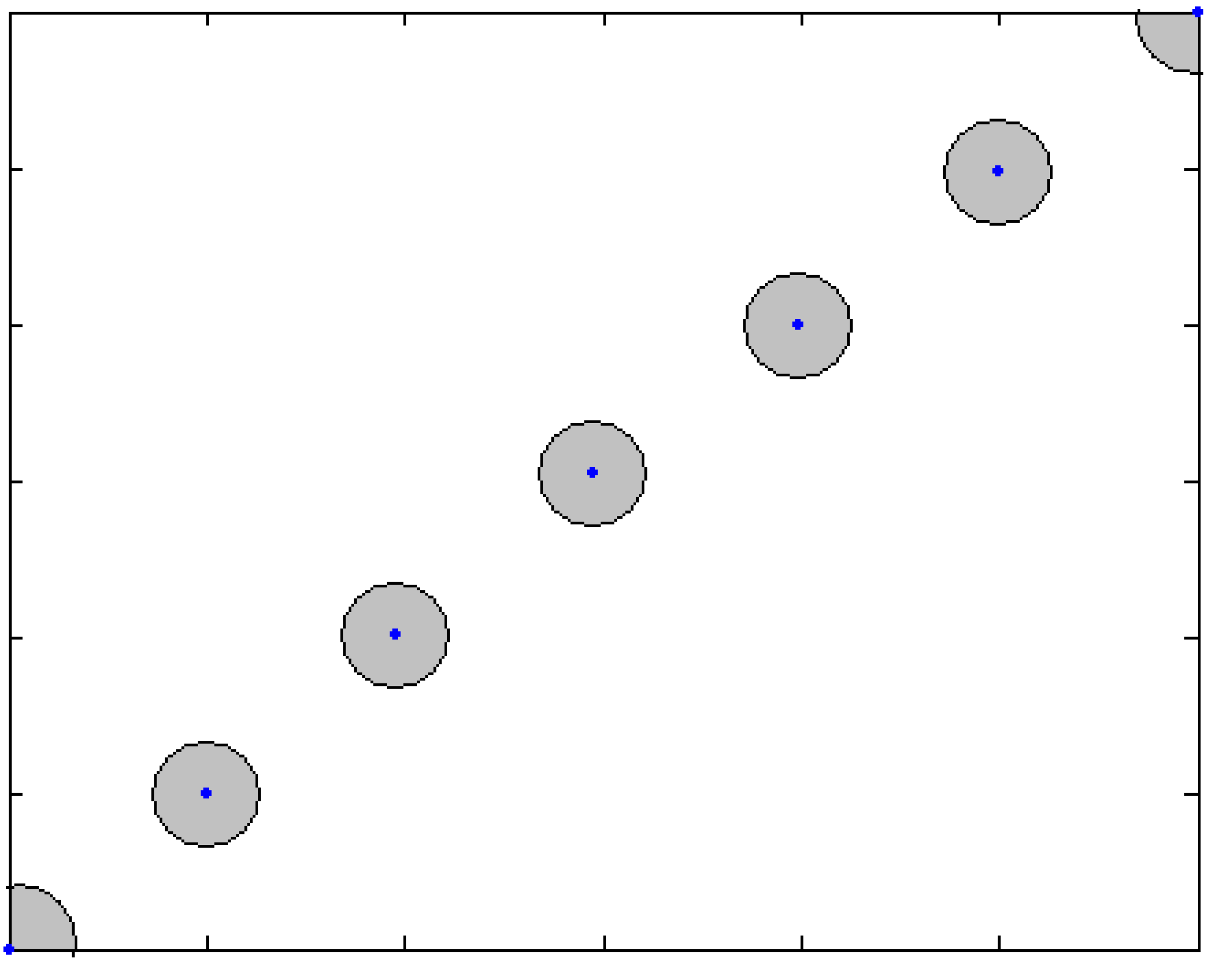
In many real applications, the area to be monitored is more extensive with respect to sensor network power sensing, m > >n. This leads to an initial dislocation that we can consider
blind, because in our polytope space, Q ⊂ ℜ
2, we suppose the equiprobability for the occurrence of a pollution event. For example, in
Figure 4 is shown a linear dislocation of seven sensors with a limited sensing radius (gray circles). We want to cover the maximum area with the lowest number of wireless sensors moving in a large area. The general characteristics of the mobility for the wireless sensors should meet this general requirement; nevertheless, large portions of the unchecked areas must be taken into consideration.
When a pollution event takes place, the sensors move in the direction of the pollutant slick, re-dislocating themselves in a Voronoi set centroid given by the knowledge of some environmental information. The environment changes the shape of the slick, expressed by ρ(|q-pi|,t), making it asymmetrical; consequently, the new dislocation implies that the new centroids overlap the individual sensing radii; i.e., Ri − Rj < R, with i, j = 1…n, enforcing their power sensing in one direction rather than another one. The first step is a fast dislocation of a single sensor; for example, the sensor nearest to the pollution event. The control law (Equation (12)) is integrated calculating the centroids at regular steps, once a pollution event has been located. The convergence is guaranteed by choosing an effective α parameter as ≥ 10 and time steps for the calculation of the new centroids set proportional to α/5.
In
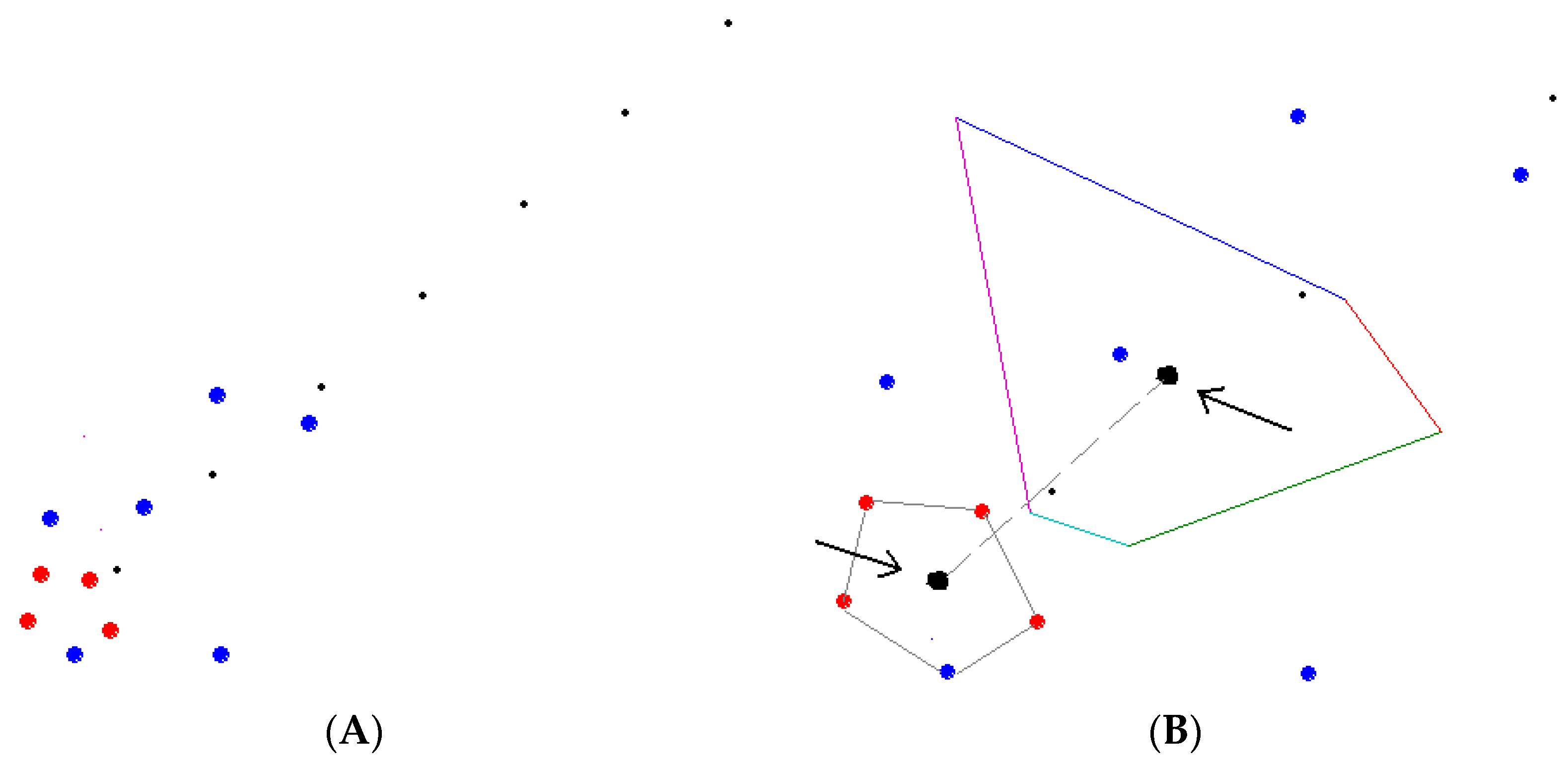
Figure 5 the main results of our procedure are represented. The blind dislocation is changed as a function of pollutions events. In our case, we limited ourselves to a single pollution event moving but unchanging shape. The two localizations and the correspondent dislocations of sensor networks are displayed in
Figure 5A and zoomed-in in
Figure 5B. In a first approach, the blind dislocation is changed considering that the pollution event is localized at a point described by a Poisson distribution, where the pollution event and the other ones by the sensors occupy one site, following the Voronoi tessellation. The sensor nearest to the pollution event is locked and the other sensors are moved to be collocated at the positions identified by the centroids set calculated with the Equation (13). As the slick moves, the configuration of the sensor network is defined by the new centroids set, where at any new calculation, the nearest sensors are locked. The final result is reached when the sensing power is maximal. The sensing power is defined by the functions
for r < R
i, and
otherwise. In
Figure 5B, the final configuration is obtained by the five sensors forming a pentagon; the blue point denotes the sensors that in the preview centroids set were locked because of being nearest to the slick. The results in
Figure 5 were obtained taking the parameter α = 10; i.e., the sensor velocity has been taken to be ten times the slick velocity, a slow diffusion regime. This guarantees the fast converge to the centroids set without complicating the configuration due to the slick shift during the sensor dislocation. It is evident that the parameter α includes the main characteristics of the diffusion process. Fast dynamics of the slick, with fast changes of position and shape of the slick, would be useless without our algorithm.
All the numerical results were obtained by writing an original Matlab program. The presented results are rather general and they can be applied to many real situations when a priori knowledge of the environments to be monitored is unavailable. If a priori knowledge on where a pollution event can take place and the diffusion process, expressed by ρ(|q-pi|,t), is not available, the initial configuration of the sensors can be well simulated using the Poisson distribution of the random events for the centroids set. In such situations of real uncertainty, some improvements for our algorithm can be made conjugating the centroidal Voronoi tessellations with an inferential approach, but this is beyond the scope of the present paper.


