Abstract
This paper describes a new set of experiments focused on estimating time series of the free surface elevation of water (FSEW) from velocities recorded by submerged air bubbles under regular and irregular waves using a low-cost non-intrusive technique. The main purpose is to compute wave heights and periods using time series of velocities recorded at any depth. The velocities were taken from the tracking of a bubble curtain with only one high-speed digital video camera and a bubble generator. These experiments eliminate the need of intrusive instruments while the methodology can also be applied if the free surface is not visible or even if only part of the depth can be recorded. The estimation of the FSEW was successful for regular waves and reasonably accurate for irregular waves. Moreover, the algorithm to reconstruct the FSEW showed better results for larger wave amplitudes.
1. Introduction
The kinematic study of the free surface elevation of water (FSEW) is the main data source to estimate the wave velocities and forces acting on maritime infrastructure. The measurement of the FSEW with non-intrusive techniques is one of the most challenging topics in the field of Coastal Engineering and Fluid Dynamics. Over the last 30 years, a vast number of research studies on the behavior of the FSEW of irregular waves have been carried out. The authors of [1] presented a comparison between mathematical and laboratory measurements of velocities below the FSEW with a laser Doppler velocimeter (LDV) to compute the wave forces on submarine pipelines. In this work, water level fluctuations were measured to calculate the time series of velocities. The same set of experiments was replicated with inductive- and impeller-type probes instead of an LDV to confirm the theories with the prediction of velocities and pressures by [2,3]. These authors also estimated the FSEW using pressure data. In [4], a transfer function was obtained to estimate the surface from pressure measurements in deep water. Later, [5] compared the theory and measurements of water particle velocities in solitary waves, while [6] carried out the same experiments under monochromatic waves.
Calculations of spectral transfer functions between the FSEW and subsurface 3D particle velocities in wind-induced waves were also performed by [7]. Other researchers also measured water particle velocities and water surface elevations [8,9,10,11]. In addition, measurements of pressure under irregular waves were taken to estimate the water depth at several positions [12,13]. Pressure-, capacitance-, and resistance-type wave gauges were used by [14] in traditional detection of FSEW.
These techniques usually constitute discrete localized point measurements; hence, the recorded data are not enough to understand the behavior of the water surface. Due to these limitations, new optical techniques to measure the FSEW were developed to obtain more accurate datasets regarding time and space. The authors of [15] created a new technique combining colorimetry and digital image processing to obtain the 3D free surface elevation for a time-dependent flow. The authors of [16] developed a new technique to measure two components of the water surface gradient and, subsequently, [17] created an algorithm for the estimation of water surface elevation by integrating the surface gradient.
By that time, the measurements of velocity fields (e.g., [18]) were obtained using imaging techniques, such as laser speckle velocimetry (LSV), particle imaging velocimetry (PIV), particle tracking velocimetry (PTV), defocusing digital particle image velocity (DPIV), stereo photography, shadowgraphy, laser slope gauges, and optical displacement sensors as diffusing light photography by [19,20], who measured deflection of a reflected laser beam on the free surface at each point.
Fringe projection profilometry was used by [21] to measure the FSEW, while [22] broadened the study into the well-known Fourier transform profilometry (FTP). This technique was later combined with digital PIV [23,24] to study the relationship between small-sloped FSEW deformations and near-surface velocities. Based on laser speckle techniques, [25] developed a system to measure the distortion of a collimated speckle pattern. In addition to these techniques, [26,27] developed two different stereoscopic methods for measuring 2D water surface elevations. [28] used dynamic refraction stereo to estimate an unknown refractive 3D water surface. More recently, [29] used phase shifting and FTP to estimate the FSEW in a 3D flow. Later, [30,31] performed simultaneous measurements of topography and velocity fields on FSEW and [32] analyzed a refracted image and a reference image to measure the FSEW. Other research studies measured the deformation of the FSEW with a modification to the optical profilometry technique [33] and measured the flow fields beneath the free surface of the waves with PTV [34,35]; [36,37] also used PTV to measure wave-induced mean flow and particle trajectories for linear wave packets. In turn, [38] used PIV methods to evaluate mass transport velocity based on measured vector fields. A theoretical study recently was made to predict the surface waves following the recovery of the pressure at the bottom [39].
It can thus be seen a growing interest in understanding and characterizing the FSEW to find the relationships between wave hydrodynamics and other related parameters such as wave energy, pressure, velocities, and vertical acceleration below the free surface, the forces which deform the FSEW in the presence of coastal structures, etc.
Despite these efforts to improve the measurements, some methods interfere with the FSEW. For example, wave gauges can act as obstacles for the free surface, consequently altering the behavior of the wave. On the other hand, non-intrusive water surface visualization has been limited to optical techniques [40]. Bubble image velocimetry (BIV) techniques have been adopted by various researchers to obtain the velocity of bubbles generated by air entrapment and entrainment of breaking and broken waves to study wave hydrodynamics and overtopping [41,42] as well as kinematics around pneumatic breakwaters [43]. Nevertheless, as the bubbles were of different sizes, shapes, and buoyancy forces, the application of the BIV technique or algorithm was hindered in some cases. Other research studies of the velocity of bubbles were carried out using electrolysis, the measurement of the vertical distributions of the water particle velocity induced at a certain wave phase [44]. Another measurement technique was using the defocusing of digital particle images to calculate the velocity field from the cross-correlation of volumes from two sequential defocusing bubble images [45]. There have also been studies on the characteristics of bubbles rising in water; i.e., velocity, trajectory, oscillation frequency, size, and density [46,47,48,49].
The main purpose of the present study is to use a non-intrusive technique that measures the velocities of a curtain of artificially created bubbles. The bubbles were generated with compressed air using a device made in-house that was placed at the bottom of the flume. The velocity of the bubbles is considered as a proxy of the water velocity and thus a transfer function was used to compute the FSEW from the time series of the velocity recorded at a known depth. Conventional techniques (wave gauges, UVP, and PIV) were used to validate the proposed methodology and to establish the depth and period ranges for which better results were obtained.
2. Materials and Methods
The experimental program was carried out in the wave flume of the National Autonomous University of Mexico (UNAM), which is 37.0 m long, 0.79 m wide, and 1.2 m deep. The flume is constructed of tempered glass walls and the wave paddle is equipped with an active absorption system to reduce the re-reflected waves. The bubble device consisted of an acrylic tube 0.80 m long, a diameter of 0.0254 m and 0.006 m thick. The device had 1 mm diameter holes separated half a centimeter along its length. The ends of the tube were hermetically sealed, and the air was supplied by a compressor connected to the central part of the tube. The pressure of the compressor was set to ensure the proper number, size, and visibility of the bubbles.
The bubble generator was placed at the bottom of the flume, centered along the channel and parallel to the wave direction. The distance from the device to the dissipative beach at the end of the flume, as shown in Figure 1 and Figure 2, was 9 m. To record the motion of the bubbles, a high-speed digital video camera set to 12,000 fps and a lens 25 mm wide were located parallel to the flume, 3.7 m away from the curtain of bubbles. The bubble curtain was illuminated by LED lamps and a black background was placed to enhance the contrast. Five wave gauges were located along the flume. The first one was placed 4.0 m away from the wavemaker paddle as a witness of the generated waves and the other four gauges were placed within the bubble curtain.
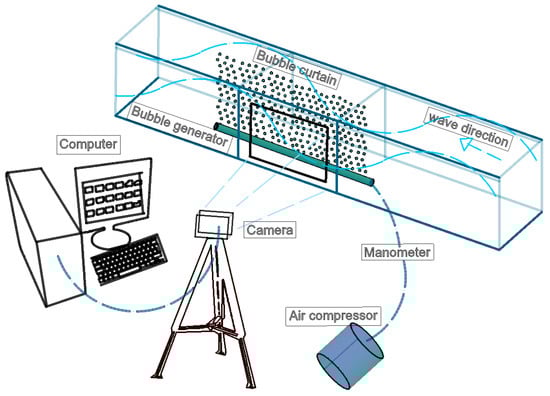
Figure 1.
Experimental setup used to record the velocity of air bubbles beneath superficial waves.
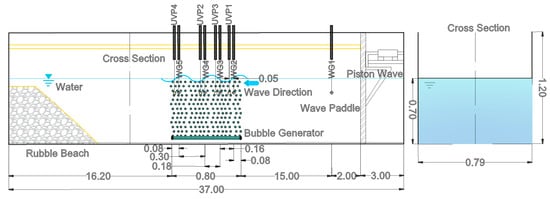
Figure 2.
Wave flume cross section. WG stands for wave gauge and UVP for ultrasonic velocity profiler. Dimensions are in meters.
Three velocity profiles were recorded using an ultrasonic velocity profiler (UVP) located close to each of the four-wave gauges and laser PIV velocity maps were used to validate the velocity fields obtained tracking the air bubbles.
3. Methodology
The experiments were performed with a still water reference depth of 0.7 m. The FSEW was perturbed by regular and irregular waves (Jonswap spectrum with γ = 3.3) with different wave heights and periods as given in Table 1. The wave trains were chosen focusing on covering a wide range of conditions, always within linear wave conditions, in order to achieve sensibility regarding the applicability of the technique for estimation of FSEW. A total of 32 tests were conducted, 16 different waves trains (8 regular and 8 irregular), were measured and each test was repeated two times.

Table 1.
Wave conditions used in present study. R and I denote regular and irregular waves, respectively.
To record the motion of the bubbles, the high-speed digital video camera was focused on the plane of the bubble curtain and series of 10,390 images were recorded. The pre-processing of the imagery consisted on three stages to enhance the contrast and highlight and define the bubbles, particularly the smallest bubbles that seemed blurred. First, the size of the picture was trimmed from 644 × 400 pixels (original size of the picture) to 397 × 222 pixels to capture the study area. Second, the background was captured without bubbles, and its average was subtracted from the images to eliminate any other source of light that does not correspond to the bubbles. Third, the bubbles were recorded without waves to calculate an average velocity field of the ascending motion that was subtracted from the velocity fields of the bubbles with waves.
To scale the images, a metric scale was located in the plane of the bubble curtain to find the conversion factor to be introduced later in the calculations of the velocity field. The size of a pixel in the picture resulted in 1 px = 0.00195 ± 0.0005 m. Given that the sampling frequency was 250 Hz, the conversion factor px/frame to m/s was estimated as 0.4875 ± 0.0005 m/s and the duration of each test was 41.56 s. The duration of the test allowed to record 34 waves of 1.2 s. The wave gauges were set with a sampling frequency of 100 Hz (accuracy of the sensors is 0.1 mm).
These photographs were analyzed with PIVLab code [50], employing a single frame and three interrogation window sizes: 64 × 32, 32 × 16, and 16 × 8 pixels to construct the velocity field. Additionally, the correlations between windows were made with a Fourier transform, a deformation linear window, and a Gaussian subpixel estimator. For the missing vectors, a spline interpolation method was applied. The total number of photographs in each test was 10390; this means that after applying the PIVLab analysis, 5195 velocity fields were obtained which are more than enough for the proposed analysis. The time series values were obtained as the average of a selected region at a fixed depth. Figure 3 shows an image of a velocity field where different depths have been marked; time series of velocities were taken at these depths.
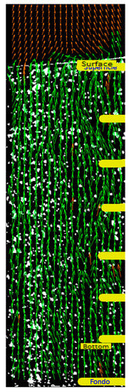
Figure 3.
Photograph processed with particle imaging velocimetry (PIV). The green vectors are the velocities of the bubbles and the red vector are the vectors interpolated due to a missing data.
For validation purposes, the FSEW was recorded both with the wave gauges and from the photographs using the Sobel operator to detect edges or borders in images.
Singular spectrum analysis (SSA) was used to remove high-frequency oscillations from the time series, and its Fourier spectrum was calculated for the two time series: one from the velocity of the bubbles (sampled at 250 Hz) and other from the wave gauges (sampled at 100 Hz). As the sampling frequencies were dissimilar, one point every 5 and one point every 2 were used from the bubble and wave gauge time series, respectively, for the comparison. A linear adjustment between the coefficients of the harmonic components of the Fourier spectra of the two time series was computed. This adjusted relationship corresponds to the transfer function which allows the FSEW to be estimated from the time series of the velocities of the bubbles.
4. Results and Discussion
To obtain the pixels corresponding to the position of the FSEW, the contour found for the still water level was used as a reference. Then, the FSEW recorded by the wave gauges and the contour in the photographs were compared.
Figure 4 compares the two time series (wave gauges and contours in the recorded images) of the FSEW. The mean absolute percentage error resulted in 5.5%, showing that an accurate estimation of the FSEW from the photographs is easy to achieve. Between the records, a phase shift exists due to the different start of the records and, therefore, an algorithm was created to match the initial time of each record and accomplish an appropriate comparison.
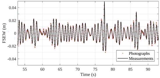
Figure 4.
Comparison of free surface elevation of water (FSEW) recorded by wave gauges and extracted from the images for Tp = 0.08 s and Hs = 0.05 m, case I3-05.
The main results were derived from the time series of velocity field from the PIVLab analysis. Figure 5 presents the time series of the regular waves case T = 0.8 s and H = 0.05 m, whereas Figure 6 shows the data for irregular waves with Tp = 0.8 s and Hs = 0.05 m. It is important to mention that these time series were constructed using all the pixels across the width of the photograph (222 pixels or 0.433 m) at 4 cm depth. The values estimated for H and T from the FSEW obtained via the image analysis were very similar to the actual generated values. The error was found to be inversely proportional to wave height and period.
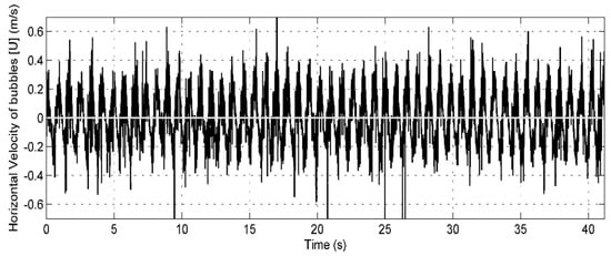
Figure 5.
Time series of the horizontal velocity of the bubbles for regular waves with H = 0.05 m and T = 0.8 s; the depth is 4 cm.
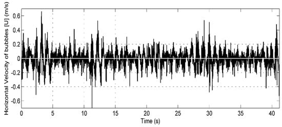
Figure 6.
Time series of the horizontal velocity of the bubbles for irregular wave with Hs = 0.05 m and Tp = 0.8 s; the depth is 4 cm.
To understand the scope of the technique, the wave heights and the periods were classified into three types according to the amplitude and period as high (0.10 m, 1.2 s), medium (0.05 m, 0.8 s), and small (0.01 m, 0.8 s), as illustrated in Table 2.
Table 2.
Summary of experimental wave parameters used in present study.
The Ursell number and two non-dimensional parameters (H/gT2 and h/gT2) were calculated to identify the Stokes order of each case. This was carried out regardless of the behavior of the waves and, hence, the bubbles detected the presence of waves.
The Fourier spectra of the time series of the bubbles and the FSEW obtained from the contours of the pictures, for regular waves, were computed to compare the frequencies in one spectrum and the other. For that reason, 20 spectra at different water depths were calculated and normalized by the maximum value.
In Figure 7a,b, the bubbles in regular waves responded according to the perturbation caused due to waves because the 20 spectra had the same shape among them, the same bandwidth, and their difference in magnitude was not large. This means that the time series of the velocities of the bubbles immediately below the FSEW gave better results than the time series close to the bottom. Figure 7e shows the Fourier spectrum obtained by the time series measured by the photographs (or if it is the case by the wave gauges) which agrees with the Fourier spectrum obtained by the 20 times series of the velocities of the bubbles (Figure 7a,b).
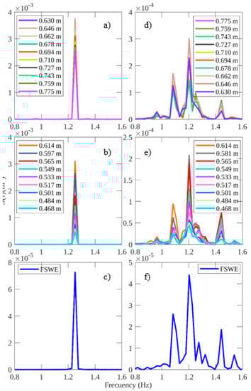
Figure 7.
Fourier spectra for (a) regular waves H = 0.05 m and T = 0.08 s using the time series of the velocities of the bubbles for depths ranging from 0.630 to 0.775; (b) regular waves H = 0.05 m and T = 0.08 s using the time series of the velocities of the bubbles for depths ranging from 0.468 to 0.614 m; (c) regular waves H = 0.05 m and T = 0.08 s using the time series of the FSEW obtained from the contours of the photographs; (d) irregular waves Hs = 0.05 m and Tp = 0.08 s using the time series of the velocities of the bubbles for depths ranging from 0.630 to 0.775 m; (e) irregular waves Hs = 0.05 m and Tp = 0.08 s using the time series of the velocities of the bubbles for depths ranging from 0.468 to 0.614 m; and (f) irregular waves Hs = 0.05 m and Tp = 0.08 s using the time series of the FSEW obtained from the contours of the photographs.
Figure 7c,d,f shows the Fourier spectra for irregular wave test cases. In this case, the spectra show multiple peaks. It is important to note that the maximum peak frequency is in good agreement with the initial frequency of the experiment. As mentioned before, 20 Fourier spectra were calculated corresponding to different water depths. The behavior of the frequencies shows that the energy decreases as the water depth decreases, but the peak frequency is always present in each spectrum meaning that up to a certain water depth, the bubbles result in good detection of the peak period of the waves.
After the calculation of the FFT of the time series of the velocities of the bubbles and of the FFT of the FSEW measured from the contours of the photographs, a scatter plot was made for the set of data to fit a transfer function, which allows computing the estimation of the FSEW. This process was repeated for regular (Figure 8) and irregular waves (Figure 9). In addition, the squared linear correlation coefficient (R2) was obtained for different water depths, going from the surface (4 cm depth) to the bottom (0.347 m depth). From these, it can be observed that the technique works better for the series of velocities of the bubbles which are found closer to FSEW. This is because the forcing of the wave diminishes with the depth. Hence, bubbles at the bottom are less influenced by the oscillatory motion than the bubbles in smaller depths.
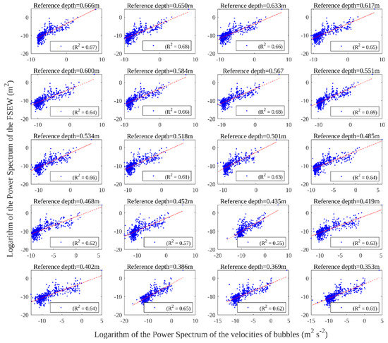
Figure 8.
Relationship between the Fourier spectrum of the time series of the velocities of the bubbles and the Fourier spectrum of the FSEW measured for regular waves with H = 0.05 m and T = 0.08 s.
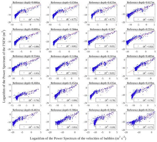
Figure 9.
Relationship between the Fourier spectrum of the time series of the velocities of the bubbles and the Fourier spectrum of the FSEW measured for irregular waves with Hs = 0.05 m and Tp = 0.08 s.
The range of valid time series along the depth was chosen from 0.04 to 0.347 m depth. Closer to the free surface than the first limit, the PIV velocity fields are not properly estimated due to the lack of bubble neighbors in the images. The second limit is the threshold for which acceptable error was found in the wave period results. The R2 values in Figure 8 and Figure 9 are similar for the different water depths and no trend can be seen, indicating that R2 is independent of the depth; this means that the technique can be used with the same accuracy for any depth within the valid range. Globally, despite R2 having consistent values, it is also observed that especially for irregular waves, some frequencies are far from the linear adjustment and it has not been studied yet if any of these frequencies can improve the estimation of the FSEW.
The estimations of the FSEW were obtained from velocity data at different depths with transfer functions. These transfer functions were calculated by adjusting the power spectra of the time series of the velocities of the bubbles and the power spectra of the time series of the FSEW obtained with the contours from the photographs. The linear adjustment between the two power spectra in a log–log scale relates the coefficients of the amplitude of each Fourier harmonic between the two spectra. Hence, each harmonic of the time series of the velocity of the bubbles was adjusted to obtain the values of each harmonic of the FSEW. The power spectrum is defined as the absolute value of the square of the Fourier transform coefficients.
As shown in Figure 10 and Figure 11, for regular waves, the estimated (Reconstructed) and measured FSEW obtained from the contours of the photographs (Target) are similar, except for 0.29 m depth. Hence, it is found that this depth is a threshold depth that defines where the technique stops working. For the irregular waves, the most significant difference between the reconstructed and target curves occurred when the FSEW reaches its largest absolute values, or when there is a small or large change in the amplitude. The comparison of the FSEW can be considered accurate enough because the mean error calculated with the six-time series presented in Figure 10 was of ±0.0025 m for regular waves and ±0.004 m for irregular waves. The mean error is defined as the mean of the absolute value of the subtraction between the two curves (FSEW Target − FSEW Reconstructed). If it is considered H = 0.05 m, then the error for regular waves was 5% and for irregular waves was 8%.
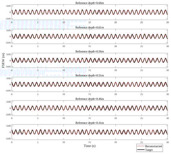
Figure 10.
Measured and estimated FSEW for regular waves with H = 0.05 m and T = 0.08 s.
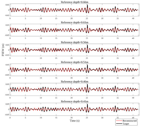
Figure 11.
Measured and estimated FSEW for irregular waves with Hs = 0.05 m and Tp = 0.08 s.
Figure 12 summarizes the results obtained for the cases of the Table 1 for irregular waves. There, the relationship between R2 and the Relative Depth (0 corresponds to the still water level and 1 corresponds to the bottom) is shown. The term R2 is defined as the squared linear correlation coefficient of the reconstructed FSEW (Reconstructed) and the measured FSEW (Target). For the cases where the wave heights are 0.1 and 0.05 m and the periods are 0.8 and 1.2 s, a clear trend is observed such that as the depths decrease, the R2 values decrease dramatically. The same abrupt change is found for wave heights of 0.03 and 0.01 m and periods of 0.8 and 1.2 s. Nevertheless, the curves for 0.01 m wave heights do not clearly show this abrupt change. However, for some water depths, the velocity field of the air bubbles is a good predictor of the FSEW.
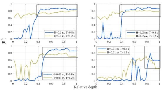
Figure 12.
Critical curves defined as the squared linear correlation coefficients (R2) as a function of relative depth for different wave periods and wave heights.
The correlation values decrease with depth. Arguably, this is due to the closeness to the bubble generator where the velocity of the bubbles is dominated by their vertical displacement and thus no velocity related to the waves can be measured. The curves of Figure 12 reveal zones where the technique works, and the bubbles are sufficiently influenced by the waves such that they carry enough information to reconstruct the FSEW.
5. Conclusions
The technique employed to estimate the FSEW through the velocity field of the air bubbles gave good results (for a range of depths) compared to traditional measuring methods. The horizontal motion of the bubbles can also serve as a proxy to the motion of the water particles in coastal waves. Beyond reconstruction of the FSEW, the paper focuses on the relationship between the spectral peaks of the horizontal velocities of the air bubbles and of the FSEW.
Hence, it was observed that for regular waves, the oscillating movement of the air bubbles was in accordance with the wave period, whereas the velocities and periods of oscillation of the bubbles under irregular waves coincided with the range of the periods found in the irregular wave train. The critical curves obtained for different initial conditions describe the depths where the technique is valid. In our experiments, it was observed that for 0.7 m depth, wave amplitudes of 0.1 m, and periods of 1.2 s, the technique works well for depths lower than 0.4 m excluding subsurface area. It should be noted that for depths of around 0.03 m, the time series of the bubble velocities shows some irregularities. Arguably, this zone is behaving as a boundary layer between water and air.
The results show that the technique does not work very well to determine the FSEW when there is an abrupt change in the wave amplitude, for example, as shown in Figure 9 at 25 s.
The proposed non-intrusive methodology is useful in 2D wave flumes where it is desirable to obtain the FSEW without the use of typical wave gauges as well as to determine the behavior of the velocity of water particles that are below the FSEW. Moreover, the bubble generator is user-friendly and economical compared to a wave gauge. By contrast, it requires precise coupling between the speed of the camera, the control of bubble velocities, and the magnitude of fluid velocity.
A plan for future study is to perform more experiments within the range under which the technique is valid, in terms of the total depth, amplitudes, and periods. Moreover, it is recommended that the response time of the bubbles under different wave forcing effects be studied, for example, during wave breaking, where mass transport could play a significant role and could be important for FSEW reconstruction using the proposed technique.
Author Contributions
Conceptualization, D.V. and R.S.; methodology, R.J. and D.V.; software, D.V. and E.M.; validation, D.V. and E.M.; formal analysis, E.M. and R.J.; investigation, D.V.; resources, R.S. and R.J.; data curation, D.V.; writing—original draft preparation, D.V. and E.M.; writing—review and editing, R.J., E.M. and R.S.; visualization, D.V.; supervision, R.S. All authors have read and agreed to the published version of the manuscript.
Funding
This research received no external funding.
Acknowledgments
The data analysis of the proposed work was carried out at the University of East London (UEL) while spending postgraduate student internship of the first author. Therefore, the authors are grateful for the computing facilities and laboratory space provided by the UEL. The authors would also like to thank CEMIE-Oceano (CONACYT grant no. 249795) for partially funding this research.
Conflicts of Interest
The authors declare no conflict of interest.
References
- Vis, F.C. Orbital velocities in irregular waves. In Proceedings of the 17th Coastal Engineering Conference, Sydney, Australia, 23–28 March 1980; pp. 173–185. [Google Scholar]
- Daemrich, K.-F.; Eggert, W.-D.; Kolhase, S. Investigations on irregular waves in hydraulic models. In Proceedings of the 17th Coastal Engineering Conference, Sidney, Australia, 23–28 March 1980; pp. 186–203. [Google Scholar]
- Daemrich, K.F.; Eggert, W.-D.; Cordes, H. Investigations on orbital velocities and pressures in irregular waves. In Proceedings of the 18th Coastal Engineering Conference, Cape Town, South Africa, 14–19 November 1982; pp. 297–311. [Google Scholar]
- Lee, D.-Y.; Wang, H. Measurement of surface waves from subsurface gauge. In Proceedings of the 19th International Conference on Coastal Engineering, Houston, TX, USA, 3–7 September 1984; pp. 271–286. [Google Scholar]
- Lee, J.-J.; Skjelbreia, J.M.; Raichlen, F. Measurement of velocities in solitary waves. J. Waterw. Port C. Div. 1982, 108, 200–218. [Google Scholar]
- Bullock, G.N. Short I. Water particle velocities in regular waves. J. Waterw. Port C. Ocean Eng. 1985, 111, 89–200. [Google Scholar]
- Battjes, J.A.; Van Heteren, J. Verification of linear theory for particle velocities in wind waves based on field measurements. Appl. Ocean Res. 1984, 6, 187–196. [Google Scholar] [CrossRef]
- Swan, C. Convection within an experimental wave flume. J. Hydraul. Res. 1980, 28, 273–282. [Google Scholar] [CrossRef]
- Hansen, J.B. Periodic waves in the surf zone: Analysis of experimental data. Coast. Eng. 1990, 14, 19–41. [Google Scholar] [CrossRef]
- Kim, C.H.; Randall, R.E.; Krafft, M.J.; Boo, S.Y. Experimental study of kinematics of large transient wave in 2D wave tank. In Proceedings of the 22nd Annual Offshore Technology Conference, Houston, TX, USA, 7–10 May 1990; pp. 195–202. [Google Scholar]
- Zhang, J.; Randall, R.E.; Spell, C.A. On wave kinematics approximate methods. In Proceedings of the 23rd Annual Offshore Technology Conference, Houston, TX, USA, 6–9 May 1991; pp. 231–238. [Google Scholar]
- Nielsen, P. Local approximations: A new way of dealing with irregular waves. In Proceedings of the 20th International Conference on Coastal Engineering, Taipei, Taiwan, 9–14 November 1986; pp. 633–646. [Google Scholar]
- Bergan, P.O.; Torum, A.; Tratteberg, A. Wave measurements by a pressure type wave gauge. In Proceedings of the 11th International Conference on Coastal Engineering, London, UK, September 1968; pp. 19–29. [Google Scholar]
- Jahne, B.; Klinke, J.; Waas, S. Imaging of short ocean wind waves: A critical theoretical review. J. Opt. Soc. Am. 1994, 11, 2197–2209. [Google Scholar] [CrossRef]
- Zhang, X.; Dabiri, D.; Gharib, M. A novel technique for free-surface elevation mapping. Phys. Fluids 1994, 6, S11. [Google Scholar] [CrossRef][Green Version]
- Zhang, X.; Cox, C.S. Measuring the two-dimensional structure of a wavy water surface optically: A surface gradient detector. Exp. Fluids 1994, 17, 17–225. [Google Scholar] [CrossRef]
- Zhang, X. An algorithm for calculating water surface elevations from surface gradient image data. Exp. Fluids 1996, 21, 43–48. [Google Scholar] [CrossRef]
- Adrian, R.J. Particle-imaging techniques for experimental fluid mechanics. Annu. Rev. Fluid Mech. 1991, 23, 261–304. [Google Scholar] [CrossRef]
- Wright, W.B.; Budakian, R.; Putterman, S.J. Diffusing light photography of fully developed isotropic ripple turbulence. Phys. Rev. Lett. 1996, 76, 4528–4531. [Google Scholar] [CrossRef] [PubMed]
- Vivanco, F.; Melo, F. Experimental study of surface waves scattering by a single vortex and a vortex dipole. Phys. Rev. 2004, 69, 1–12. [Google Scholar] [CrossRef] [PubMed]
- Grant, I.; Stewart, N.; Padilla-Perez, I.A. Topographical measurements of water waves using the projection moire method. Appl. Optics 1990, 29, 3981–3983. [Google Scholar] [CrossRef] [PubMed]
- Zhang, Q.-C.; Su, X.-Y. An optical measurement of vortex shape at a free surface. Opt. Laser Technol. 2002, 34, 107–113. [Google Scholar] [CrossRef]
- Dabiri, D.; Gharib, M. Simultaneous free-surface deformation and near-surface velocity measurements. Exp. Fluids 2001, 30, 381–390. [Google Scholar] [CrossRef]
- Dabiri, D. On the interaction of a vertical shear layer with a free surface. J. Fluid Mech. 2003, 480, 217–232. [Google Scholar] [CrossRef]
- Tanaka, G.; Okamoto, K.; Madarame, H. Experimental investigation on the interaction between a polymer solution jet and a free surface. Exp. Fluids 2000, 29, 178–183. [Google Scholar] [CrossRef]
- Tsubaki, R.; Fujita, I. Stereoscopic measurement of a fluctuating free surface with discontinuities. Meas. Sci. Tech. 2005, 16, 1894–1902. [Google Scholar] [CrossRef]
- Benetazzo, A. Measurements of short water waves using stereo matched image sequences. Coast. Eng. 2006, 53, 1013–1032. [Google Scholar] [CrossRef]
- Morris, N.J.W.; Kutulakos, K.N. Dynamic refraction stereo. In Proceedings of the 10th IEEE International Conference on Computer Vision, Beijing, China, 17–21 October 2005; pp. 1573–1580. [Google Scholar]
- Cochard, S.; Ancey, C. Tracking the free surface of time dependent flows: Image processing for the dam-break problem. Exp. Fluids 2008, 44, 59–71. [Google Scholar] [CrossRef]
- Fouras, A.; Lo Jacono, D.; Sheard, G.J.; Hourigan, K. Measurement of instantaneous velocity and surface topography in the wake of a cylinder at low Reynolds number. J. Fluid. Struct. 2008, 24, 1271–1277. [Google Scholar] [CrossRef]
- Ng, I.; Kumar, V.; Sheard, G.J.; Hourigan, K.; Fouras, A. Experimental study of simultaneous measurement of velocity and surface topography: In the wake of a circular cylinder at low Reynolds number. Exp. Fluids 2011, 50, 587–595. [Google Scholar] [CrossRef]
- Moisy, F.; Rabaud, M.; Salsac, K. A synthetic Schlieren method for the measurement of the topography of a liquid interface. Exp. Fluids 2009, 46, 1021–1036. [Google Scholar] [CrossRef]
- Cobelli, P.J.; Maurel, A.; Pagneux, V.; Petijeans, P. Global measurement of water waves by Fourier transform profilometry. Exp. Fluids 2009, 46, 1037–1047. [Google Scholar] [CrossRef]
- Hering, F.; Leue, C.; Wierzimok, D.; Jähne, B. Particle tracking velocimetry beneath water waves. Part I: Visualization and tracking algorithms. Exp. Fluids 1997, 23, 472–482. [Google Scholar] [CrossRef]
- Hering, F.; Leue, C.; Wierzimok, D.; Jähne, B. Particle tracking velocimetry. Part II: Water waves. Exp. Fluids 1998, 24, 10–16. [Google Scholar] [CrossRef]
- Grue, J.; Kolaas, J. Experimental particle paths and drift velocity in steep waves at finite water depth. J. Fluid Mech. 2017, 810, R1. [Google Scholar] [CrossRef]
- Calvert, R.; Whittaker, C.; Raby, A.; Taylor, P.H.; Borthwick, A.G.L.; van den Bremer, T.S. Laboratory study of the wave-induced mean flow and set-down in unidirectional surface gravity wave packets on finite water depth. Phys. Rev. Fluids 2019, 4, 114801. [Google Scholar] [CrossRef]
- Henry, D.; Thomas, G.P. Prediction of the free-surface elevation for rotational water waves using the recovery of pressure at the bed. Phil. Trans. 2018, 376, 1–21. [Google Scholar] [CrossRef]
- Paprota, M.; Sulisz, W.; Reda, A. Experimental study of wave-induced mass transport. J. Hydraul. Res. 2016, 54, 423–434. [Google Scholar] [CrossRef]
- Brocher, E.; Makhsud, A. New look at the screech tone mechanism of under expanded jets. Eur. J. Mech. B-Fluid. 1997, 16, 877–891. [Google Scholar]
- Ryu, Y.; Chang, K.; Lim, H.J. Use of bubble image velocimetry for measurement of plunging wave impinging on structure and associated green water. Meas. Sci. Tech. 2005, 16, 1945–1953. [Google Scholar] [CrossRef]
- Jayaratne, R.; Hunt-Raby, A.; Bullock, G.; Bredmose, H. Individual violent overtopping events: New insights. In Proceedings of the 31th International Conference on Coastal Engineering, Hamburg, Germany, 31 August–5 September 2008; pp. 2983–2995. [Google Scholar]
- Paprota, M. Experimental study on wave-current structure around a pneumatic breakwater. J. Hydro-Environ. Res. 2017, 17, 8–17. [Google Scholar] [CrossRef]
- Iwagaki, Y.; Sakai, T. Horizontal water particle velocity of finite amplitude waves. In Proceedings of the 12th Conference on Coastal Engineering, Washington, DC, USA, 13–18 September 1970; pp. 309–325. [Google Scholar]
- Pereira, F.; Gharib, M.; Dabiri, D.; Modarress, D. Defocusing digital particle image velocimetry: A 3-component 3-dimensional DPIV measurement technique. Application to bubbly flows. Exp. Fluids 2000, 29, S078–S084. [Google Scholar] [CrossRef]
- Hassan, M.S.; Khan, M.M.K.; Rasul, M.G. A study of bubble trajectory and drag co-efficient in water and non-Newtonian fluids. WSEAS Trans. Fluid Mech. 2008, 3, 261–270. [Google Scholar]
- Smutná, K.; Wichterle, K.; Večeř, M. Oscillation frequency of bubbles moving periodically in various liquids. In Proceedings of the 35th International Conference of Slovak Society of Chemical Engineering, Tatranské Matliare, Slovakia, 26–30 May 2008; p. 196. [Google Scholar]
- Ramírez de la Torre, R.; Vargas, C.; Centeno, M.; Mendez, R.; Stern, C. Characterization of a bubble curtain for PIV measurements. In Selected Topics of Computational and Experimental Fluid Mechanics, 1st ed.; Springer: Cham, Switzerland, 2015; pp. 261–269. [Google Scholar]
- Murgana, I.; Buneab, F.; Dan, G. Experimental PIV and LIF characterization of a bubble column flow. Flow Meas. Instrum. 2017, 54, 224–235. [Google Scholar] [CrossRef]
- Thielicke, W.; Stamhuis, E.J. PIVlab towards user-friendly, affordable and accurate digital particle image velocimetry in MATLAB. J. Open Res. Softw. 2014, 2, 1–10. [Google Scholar] [CrossRef]
© 2020 by the authors. Licensee MDPI, Basel, Switzerland. This article is an open access article distributed under the terms and conditions of the Creative Commons Attribution (CC BY) license (http://creativecommons.org/licenses/by/4.0/).