Abstract
The National Ocean Service (NOS), Center for Operational Products and Services installed a Physical Oceanographic Real Time System (PORTS) in San Francisco Bay during 1998 to provide water surface elevation, currents at PORTS prediction depth as well as near-surface temperature and salinity. To complement the PORTS, a new nowcast/forecast system (consistent with NOS procedures) has been constructed. This new nowcast/forecast system is based on the Finite Volume Coastal Ocean Model (FVCOM) using a computational domain, which extends from Rio Vista on the Sacramento River and Antioch on the San Joaquin River through Suisun and San Pablo Bays and Upper and Lower San Francisco Bay out onto the continental shelf. This paper presents the FVCOM setup, testing, and validation for tidal and hindcast scenarios. In addition, the San Francisco Bay Operational Forecast System (SFBOFS) setup within the NOS Coastal Ocean Model Framework (COMF) is discussed. The SFBOFS performance during a semi-operational nowcast/forecast test period is presented and the production webpage is also briefly introduced. FVCOM, the core of SFBOFS, has been found to run robustly during the test period. Amplitudes and epochs of the M2 S2, N2, K2, K1, O1, P1, and Q1 constituents from the model tide-only simulation scenario are very close to the observed values at all stations. NOS skill assessment and RMS errors of all variables indicate that most statistical parameters pass the assessment criteria, and the model predictions are in agreement with measurements for both hindcast and semi-operational nowcast/forecast scenarios.
1. Introduction
In 1998, the National Oceanic and Atmospheric Administration (NOAA)/National Ocean Service (NOS) installed a Physical Oceanographic Real Time System (PORTS) in San Francisco Bay to provide water surface elevation, current, near-surface and near-bottom temperature and salinity, and meteorological information to promote safe and efficient navigation in this area [1]. As PORTS only supplies measured data at selected stations, NOS’ National Operational Coastal Modeling Program (NOCMP) is developing an Operational Forecast System (OFS) to complement the service.
Many researchers have employed different versions of TRIM (Tidal, Residual, Intertidal, Mudflat Model) [2,3,4] for their purposes in the bay. For example, Cheng and Smith [5] employed the TRIM2D (two-dimensional TRIM) for the San Francisco Bay Marine Nowcast. The TRIM3D was recently applied by Gross et al. [6] to the entire San Francisco Bay. The UnTRIM, an unstructured version of TRIM3D, has also been applied to San Francisco Bay by MacWilliams and Cheng [7].
Two- and three-dimensional models have been extensively applied to investigate the hydrodynamic and morphologic processes in San Francisco Bay. Barnard et al. [8,9,10] report the existence of sand waves with heights in the order of 2 meters at the entrance of the Bay and consider coastal process evolution and the numerical prediction of severe storms on the coastline initially using the two-dimensional vertically integrated mode of the Delft3D-FLOW model [11]. Uslu et al. [12] developed a very high resolution two-dimensional vertically integrated model for tsunami forecasts in this region.
Fringer et al. [13] developed the non-hydrostatic option SUNTANS (Stanford Unstructured Nonhydrostatic Terrain-following Adaptive Navier-Stokes) model, which has also been applied in San Francisco Bay by Chua and Fringer [14].
Some of these structured and unstructured models [15,16] have been employed to understand the role of stratification and baroclinic circulation on salt intrusion in the northeastern part of Figure 1. They focus on the dynamic interactions between fresh water from the Sacramento and San Joaquin Rivers and salt water from the open ocean. Their studies, as will be seen later in this paper, have great value in evaluating the advantage and disadvantage of using a flow or stage river boundary condition for these two rivers.
The primary objective of the NOCMP, however, is to develop and operate a national network of OFSs to support NOAA’s mission goals and priorities. This ongoing San Francisco Bay Operational Forecast System (SFBOFS) will become a new member of the existing OFS family. Up to now, NOCMP has successfully developed CBOFS (Chesapeake Bay), DBOFS (Delaware Bay), TBOFS (Tampa Bay), NGOFS (Northern Gulf of Mexico), CREOFS (Columbia River Estuary) and other OFSs which along the Atlantic, Gulf of Mexico, Great Lake and Pacific Coasts.
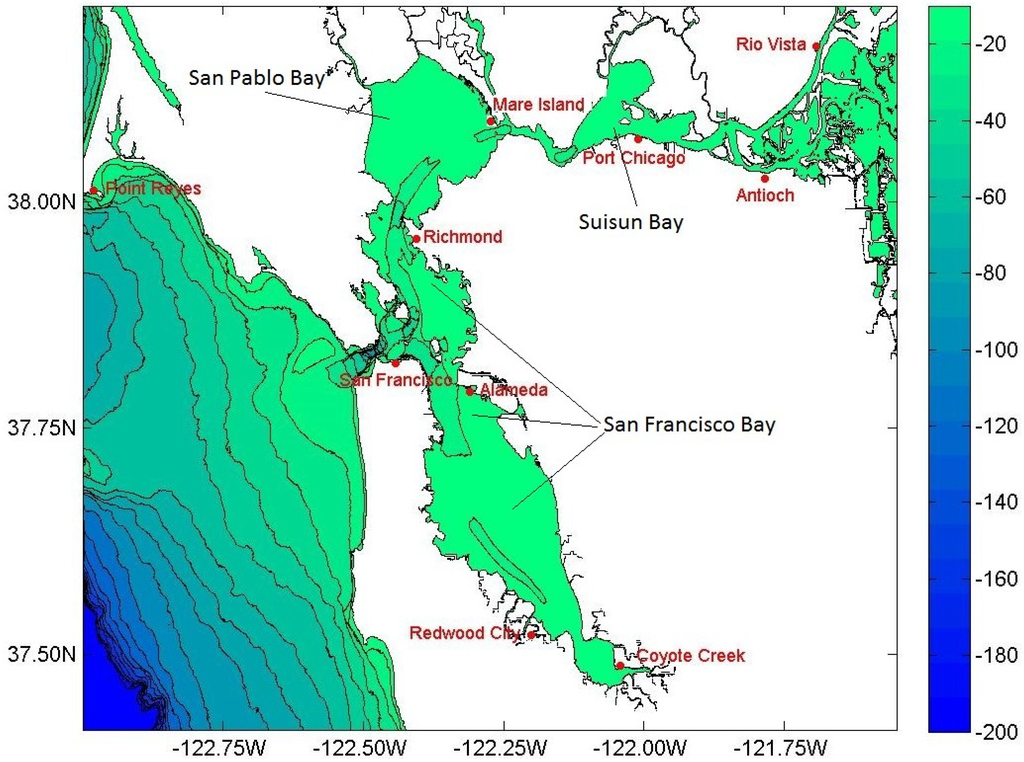
Figure 1.
The bathymetry of San Francisco Bay Operational Forecast System and the major gauge stations. The definition of “delta” in this paper is the region with complicated water channels to the east of Antioch and Rio Vista. The locations of the three major bays are indicated. Note: the domain in this figure is a little larger than the model grid domain as shown in Figure 2.
With the use of the COMF (Coastal Ocean Model Framework) on NOAA’s High Performance Computer (HPC), each OFS automatically integrates NOAA’s observing system’s data streams and the forecast output from meteorological and basin scale ocean models to generate necessary model input forcings, and then perform hydrodynamic model predictions with such forcings. Also with COMF, these OFSs perform nowcast and short-term forecast predictions (48 hours in most case) of pertinent parameters which include water levels, currents, salinity, and temperature and disseminate them to users. A state-of-the-art numerical hydrodynamic model driven by real-time data and meteorological, oceanographic, and river flow (or stage) forecasts forms the core of the end-to-end system. For detailed information on the COMF refer to Zhang et al. [17]. NOS CO-OPS is evolving to support two hydrodynamic models: ROMS for structured grid applications and FVCOM for unstructured grid applications.
As San Francisco Bay (Figure 1) has complex topography and shallow water features (the average water depth is less than 5 meters in the Bay), the well tested unstructured Finite Volume Coastal Ocean Model (FVCOM) [18,19,20] is employed as the core of the SFBOFS. Another reason to employ FVCOM lies in the fact that this model has already been ingested into the COMF-HPC as one of the major core models.
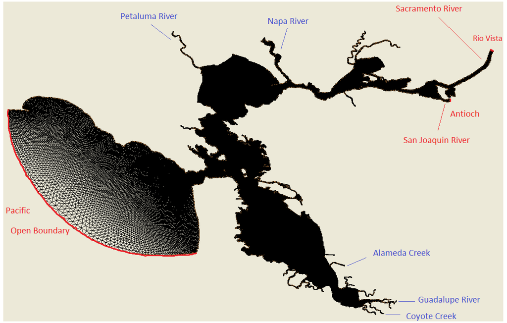
Figure 2.
The SFBOFS grid structure and the open boundaries. Measured river flow data from USGS are used as river forcings for the five small rivers in blue. Measured river flow or river stage data at Rio Vista and Antioch may be used as river forcings, respectively, for Sacramento River and San Joaquin River. Technically, if river stage data are employed, the grid points across these two major rivers are treated the same way as those on the Pacific Open Boundary.
This paper shows the major steps in how SFBOFS has been developed, assessed and put into quasi-operational status. First, FVCOM is briefly reviewed in Section 2, followed by an overview of the model’s setup in Section 3 for the tide and hindcast cases. Section 4 presents the model’s astronomical tide-only scenario simulation evaluation, while the hindcast skill assessments are described in Section 5. The COMF setup and assessment of the quasi-operational nowcast/forecast test are discussed in Section 6. Conclusions and discussion are given in Section 7.
2. The Model Overview, its Grid, and Subsequent Revisions
The physics of the FVCOM model and many aspects of the computational scheme are equivalent to the widely used Princeton Ocean Model. The FVCOM model solves the three-dimensional, vertically hydrostatic, free surface, turbulent averaged equations of motions for a variable density fluid. The model uses a triangular unstructured horizontal grid with a generalized sigma vertical coordinate. Dynamically coupled transport equations for turbulent kinetic energy, turbulent length scale, salinity and temperature are also solved. The two turbulence parameter transport equations implement the Mellor-Yamada level 2.5 turbulence closure scheme. The numerical scheme employed in FVCOM to solve the equations of motion is summarized in [18,19,20].
The FVCOM application to San Francisco Bay uses external forcing of water level, ocean density, wind, sea level atmospheric pressure, air temperature, relative humidity, downward long wave radiation, short wave radiation, and fresh water discharges entering the model domain. The model calculates water levels, three dimensional velocity, salinity, and temperature.
The horizontal grid structure and open boundaries are shown in Figure 2. This grid was developed using the Surface Water Modeling System (SMS) Version 10.1 as described by Brigham Young University Surface Modeling Laboratory and was based on the VDATUM grid developed for the coastal waters of North/Central California, Oregon and Western Washington [21]. The open boundary of the San Francisco Bay grid was developed from this grid in the near shelf region external to the Bay. It was necessary to modify the VDATUM grid such that the outer boundary of the San Francisco Bay grid follows an approximate circular arc with one of the element sides near orthogonal to the boundary arc. The grid contains 102264 elements and 54120 nodes with a minimum depth of 0.2 m and maximum depth of 106.8 m [22]. A uniform 20-layer sigma level vertical discretization was considered.
The following element quality checks were used: (1) minimum and maximum interior angles of 10 and 130 degrees, respectively, (2) maximum slope of 0.1, (3) maximum adjacent element area change ratio of 0.5, and (4) maximum number of elements connected to a node of 8. Note the slope corresponds to the maximum allowed gradient of the edge length inside the domain. The slope determines how fast the mesh size will increase toward the middle of the region. A small slope order of 0.1 means small meshes. The paving method was used, which uses an advancing front technique to fill the polygon with elements. Based on the vertex distribution on the boundaries, equilateral triangles were created on the interior to define a smaller interior polygon. Overlapping regions were removed and the process is repeated until the region is filled. Interior nodal locations are relaxed to create better quality elements. Several triangles were adjusted such that the minimum interior angle was at least 30 degrees to improve FVCOM stability. In addition, along the open boundaries, the element topology was adjusted such that each boundary element contained only one boundary side. The triangle lengths are sufficiently small, that a reasonable M2 wavelength to grid size is obtained as shown in Figure 3, where element lengths decrease from 400 to 1700 m along the open ocean boundary to a near uniform resolution of order 150 m throughout the interior bays and into the lower delta.
Several modifications were made in the development of SFBOFS to Version FVCOM 3.1.6. It should be noted that if the HEATING_CALCULATED_ON options is selected then the AIR_PRESSURE_ON option must be selected. While the sea level atmospheric pressure field is needed for the heating calculations, its gradient does not need to be applied in the momentum equations. In fact, for tidal simulations this is not correct. For tidal simulations with the heat flux calculations selected, it is necessary to provide a constant sea level atmospheric pressure field (1013 mb). Also, if one selects AIRPRESSURE_ON = F in namelist, the flag FLAG_28 = −DAIR_PRESSURE in file make.inc should be noted.
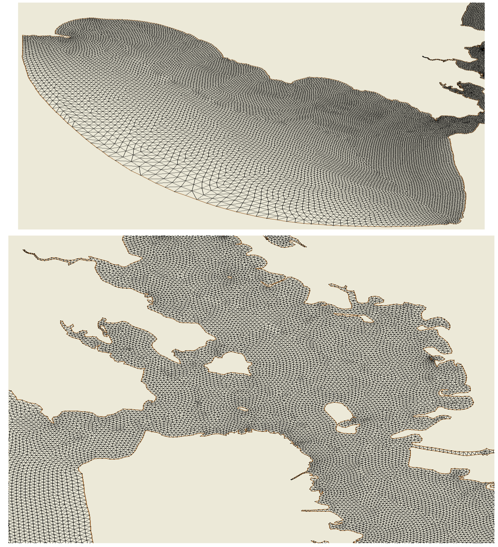
Figure 3.
The SFBOFS grid resolution structures are depicted. The element length sizes range from order 400–1700 m along the ocean boundary to order 200 m at the Bay Entrance as shown in the top panel. Within the Bay region the element lengths are reasonably uniform of order 150 m as shown in the lower panel with finer resolution around a few small islands of order 50 m.
The bottom roughness fix reported by Warner [23] for wetting/drying was added in file brough.F. In model testing, with the min_depth as 0.05 m, the model ran successfully and works for the wetting/drying case in San Francisco Bay. A Newtonian damping sponge layer was implemented by Lettmann [24], which provides a more robust implementation of the clamped water level open ocean boundary condition.
In the shallow mud flat regions of the Bay, there was also an issue with overheating. As a result, subroutine vdif_ts.F was modified to limit the short wave radiation and total heat flux as a function of depth. For depths less than 10 m, the fluxes were set to zero. In this manner, the heat transfer is due to only advection and diffusion. There, the zeta1_eff and zeta2_eff parameters which control the attenuation of the short wave radiation are set never to be less than 30% of the water depth and therefore always allow attenuation. In total, the following routines are involved in the above modifications:
- fvcom.F, mod_ncdio.F, mod_timeseries.F—air_pressure option or heating_calculated_on option.
- brough.F—bottom roughness with the Warner [23] wet/dry treatment.
- advave_edge_gcn.F, advave_edge_gcy.F, extuv_edge.F, mod_semi_implicit.F and vdif_uv.F—Lettmann [24] sponge boundary.
- vdif_ts.F and vdif_ts_gom.F—revised heat flux in shallow water.
The interaction between the hydrodynamic and the sediment-water interface, particularly in the shallow water mudflat areas, which occupy some 16% of the Bay surface area, is an area where further research is needed. Fang and Stefan [25] considered the dynamics of heat exchange between the sediment and the bottom boundary layer for several hypothetical lakes. They found that the direction of the heat transfer reverses frequently on daily timescales as well as following an overall seasonal cycle based on weather conditions at Minneapolis-St. Paul, MN. Smith [26] performed a series of heat budget studies in Indian River Lagoon, FL, to estimate the water-sediment heat exchanges using assumed values for conductivity and density. The study sought to characterize subseasonal heat fluxes and temperature changes in the sediment and overlying estuarine waters.
The bottom stress formulation in shallow water for wetting and drying has received continuing interest. Research by Xue and Due [27], Uchiyama [28], Oey [29,30], and Oey et al. [31] has indicated that the bottom drag coefficient must be adjusted if the water depth approaches the bottom roughness height. How to perform this adjustment is an area for further consideration. In the present version of FVCOM, the effective water depth used in the bottom friction formulation is limited to 3 m; e.g., when the actual water depth is less than 3 m, the depth used in the bottom friction formulation is set to 3 m.
3. Model Setup
Basically, the model needs reasonable specifications of the following four items to obtain skillful predictability. They are (1) River boundary forcing conditions, (2) open ocean boundary conditions, (3) initial conditions, and (4) surface forcings. Each of these model elements is discussed below.
3.1. River Boundary Forcing Condition Specification
There are seven rivers considered in the model. Traditional river discharge condition is used for the five small rivers that are not in the delta (the rivers with names in blue in Figure 2 and Figure 3) area. These five rivers are the Petaluma River (2 m3/s), Alameda Creek (3 m3/s), Napa River (100 m3/s), Coyote Creek (2 m3/s) and Guadalupe River (3 m3/s) with approximate mean annual flows in parentheses. The two rivers in the delta are Sacramento River at Rio Vista (1000 m3/s) and San Joaquin River at Antioch (100 m3/s) with approximate mean annual flows in parentheses. Two different upstream boundary condition types were considered for the Sacramento and San Joaquin Rivers forcing specification.
In type one, the average daily flow of Sacramento River was used to specify the flow at Rio Vista (RIO), while the San Joaquin River flow was estimated as the total delta outflow (OUT) minus the Rio Vista flow (RIO). The measured data are from the California Department of Natural Resources’ DAYFLOW [32]. The average daily flows (note: negative flow indicates flow into the Delta from the Bay) are used only for the hindcast scenario testing. Minimum inflow and zero salinity were set up for the two rivers in low flow period when DAYFLOW’s estimates may be suspect as noted by Oltmann [33]. In type two, the water level surface elevations (stage) were specified at Rio Vista and Antioch for Sacramento River and San Joaquin River, respectively, similar to the previous work in this region by MacWilliams et al. [16].
Both flow and stage river boundary conditions were used in the hindcast for comparison purposes. Please see Schmalz [22] for details. However, in the nowcast/forecast system we only use a river stage forcing for these two rivers. This is because NOCMP’s top priority is to support PORTS for navigation safety, and water level prediction is paramount. Previous studies and personal communication with Michael MacWilliams [34] have found that flow boundary condition may be more suitable if the focus is on salinity prediction. However, our major concern is surface water level as in PORTS, and the stage boundary condition is more suitable.
3.2. Open Ocean Boundary Condition Specification
The open ocean boundary of the grid (see Figure 2 and Figure 3) is forced with a superposition of the subtidal water levels and predicted tides. The harmonic constants of M2, S2, N2, K2, K1, O1, P1, and Q1 that are used to predict tide are derived from the Oregon State University Tidal Inversion Software (OTIS) for the West Coast (WC2010 1/30°) [35].
In the hindcast scenario, the subtidal water level signal at Point Reyes (see Figure 1 for its location) is used to prescribe the subtidal water level along the outer boundary. A revised sponge layer treatment at the open ocean boundary was considered. The salinity and temperature at the open boundaries were determined, with nudging, from NOAA’s World Ocean Atlas 2001 [36]. No velocities are prescribed along the open ocean boundary.
In the nowcast and forecast scenarios, subtidal water level open boundary conditions are generated from the NCEP’s (National Centers for Environmental Prediction) G-RTOFS (Global Real-Time Ocean Forecast System) gridded operational products. The temperature, salinity and baroclinic current open boundary conditions are also generated from G-RTOFS. The most recently available products for the given time period are searched and used for adjustments of the open boundary conditions using the COMF-HPC. Several horizontal interpolation methods are implemented, and a linear method is used for vertical interpolation from G-RTOFS vertical coordinates to model vertical coordinates. Measured real time sea surface elevation data at Point Reyes are used for the subtidal water level adjustment along the open boundary. Similarly, measured temperature data at San Francisco (see Figure 1 for its location) are used for boundary temperature adjustment. The adjustment is the difference between the observation and the G-RTOFS prediction at the start of the nowcast/forecast cycle and is discussed in greater detail in Section 6.1.
3.3. Initial Condition Specification
For the 19-month hindcast initial condition specification, the salinity and temperature fields were developed for 1 April 1979 using the joint NOS and USGS historical circulation survey conductivity-temperature-depth (CTD) datasets and the model was started from rest. The quasi-operational nowcast/forecast system started in the middle of March 2013 when a climatological temperature and salinity file (with adjustment from observation) was used as the very first initial condition. For each nowcast/forecast cycle, the COMF-HPC will automatically find the most recent restart file as this cycle’s initial condition (SFBOFS has four cycles a day). The details of the HPC-COMF can be found in Zhang et al. [17].
3.4. Surface Forcing Specification
For hindcast scenario, the North American Regional Reanalysis (NARR) 2007 datasets with 32 km spatial and 3 h temporal resolution were interpolated to the model grid to provide 10 m winds, sea level atmospheric pressure, and 2 m fluxes of downward shortwave radiation and net total heat flux. For the nowcast and forecast, the COMF-HPC will automatically find the most recent NAM4 (North American Mesoscale Model 4 km resolution) results in NCEP’s data tank to get the necessary input surface forcings.
4. Tidal Simulation
The tide scenario simulation is the standard first step for all OFS’ development. This is due in good measure to the fact that water level is the first priority for safe navigation, and tide and tidal current are the dominant dynamic processes in most coastal waters. For the tide scenario, the model setup for the four forcing specifications as mentioned in the previous section is similar to that for hindcast scenario. The slight differences can be found below.
4.1. Short Term Experiment: 1–15 April 1979
A three-dimensional simulation approach including baroclinics was used to capture the influence of internal waves on the tidal dynamics following [37,38]. The slight model setup difference from hindcast scenario is: winds were set to zero and the sea level atmospheric pressure set to 1013 mb. River flow conditions are used for all rivers. The April 1979 NOS and USGS historical circulation survey data were used to compare the model results with the observation.
To develop initial salinity and temperature conditions on 1 April 1979 (and on 1 September 1980 for the later extended experiment case), the available CTD and CT time series data were placed on a coarse unstructured grid of order 50 elements. An interpolation program was developed in which each FVCOM grid node was assigned a given element and the salinity/temperature value interpolated from the node values at the appropriate depths. This program allows the initial density condition to be developed for the tidal and hindcast simulations.
To calibrate the bottom roughness, the approach of Cheng et al. [15] was used, in which the bottom roughness is made a function of water depth as in Table 1. To reduce the amplitude of the simulated water level response at Port Chicago, the bottom friction was further increased above Carquinez Strait as noted in Table 1. The water level response with respect to MLLW at Port Chicago for Experiments 1 and 2 is similar (See Figure 4). Results for Experiments 5 and 7 show very minor improvement in the agreement with water level observations at Port Chicago in the order of a 2 cm reduction in RMSE. Experiments 3, 4, and 6 were unstable, due to large horizontal gradients in bottom roughness during the wetting/drying cycle.

Table 1.
Delta Inflow Bottom Friction Experiment Summary. The scale factor was used to multiply bottom roughness in model domain above Carquinez Strait. The tapered scale factor ranges from 1 to the full value in a linear fashion from Carquinez Strait to the river inflows based on longitude. The bottom roughness sets are given in the second table. The HA amplitude reduction corresponds to reducing the amplitudes of the offshore boundary harmonic constants.
| Experiment | Scale Factor | Bottom Roughness Set | HA Amplitude Reduction (%) | |
|---|---|---|---|---|
| Exp1 | 2 | 1 | 0 | |
| Exp2 | 5 | 1 | 0 | |
| Exp3 | 10 tapered | 1 | 0 | |
| Exp4 | 10 | 1 | 0 | |
| Exp5 | 5 | 1 | 5 | |
| Exp6 | 5 | 2 | 10 | |
| Exp7 | 1.2 | 2 | 10 | |
| Roughness Zone Number | Lower Depth (m) | Upper Depth (m) | Set 1 Bottom Roughness z0 (mm) | Set 2 Bottom Roughness z0 (mm) |
| 1 | 0 | 1 | 30 | 40 |
| 2 | 1 | 3 | 20 | 30 |
| 3 | 3 | 10 | 10 | 20 |
| 4 | 10 | 50 | 7 | 17 |
| 5 | 50 | 1000 | 5 | 15 |
Three additional Experiments 8–10 were conducted in which the river stage at Rio Vista and at Antioch was reconstructed from NOS harmonic constituents. Experiment 8 used the Experiment 7 bottom roughness specification. Experiment 9 included a 20 cm offset for the San Joaquin River and a 22 cm offset for the Sacramento River. In Experiment 10, the Experiment 9 offsets were retained and the Set 1 Bottom Roughness z0 values were used. Note in these stage experiments the Oregon State University Tidal Data Inversion, OTIS Regional Tide Solutions [35] harmonic analysis results were reduced by 5% for the four ocean open boundary stations. Note the Sa and Ssa harmonic constituents derived from San Francisco water level analysis were used at these stations. All other open boundary node water levels were derived via linear interpolation of values from two of the stations surrounding the node.
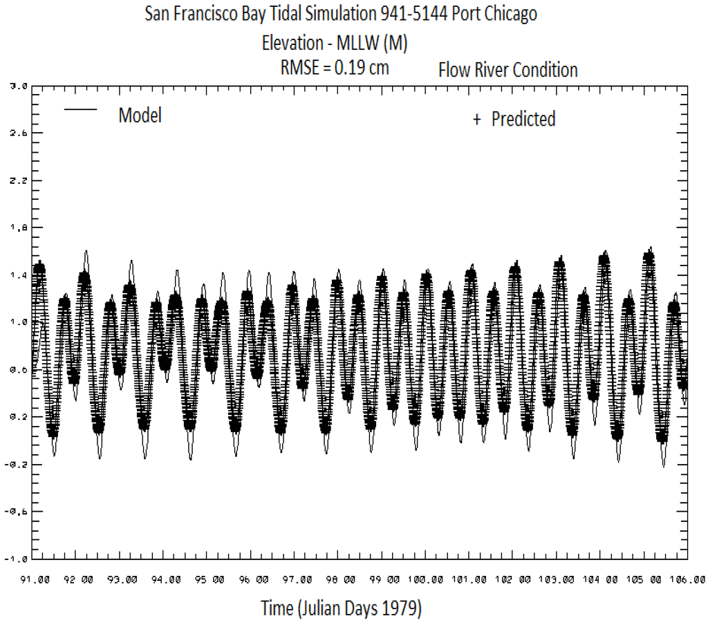
Figure 4.
Comparison of modeled versus predicted water level at Port Chicago with flow boundary condition over the period 1–15 April 1979.
In SFBOFS, we assume that the model datum is equal to the North American Vertical Datum of 1988 (NAVD88) minus 0.955 m (this resultant level is close to the MSL at open ocean boundary). Therefore, an additional field, model datum minus mean sea level, was developed. In San Francisco Bay, NAVD88 data were available from Point Reyes up to the river inflow locations.
A program was developed to access the VDATUM database and to interpolate onto the SFBOFS grid the following four datum fields: MLLW to MSL, MLW to MSL, MHHW to MSL, and MHW to MSL. In addition, the specification of the model datum (MD) to MSL allows the model predicted water level results to be presented with respect to all of the tidal datums. MSL, MLLW, NAVD88 and MSL-MD of key stations are listed in Table 2.
Note that MSL-MD difference increases from the Bay entrance to Antioch and Rio Vista. The MSL at Antioch and Rio Vista are 0.20 and 0.22 m above model datum, respectfully. The digital relationships among the different tidal datums, the model datum and NAVD88 are helpful in correctly comparing model results with measured water level data. The Experiment 10 water level response at Port Chicago with respect to MLLW is shown in Figure 5. Note by using the stage boundary condition with the offsets in Experiment 10, the agreement with observations is reduced from 19 cm in Figure 4 with the flow boundary condition to 9 cm RMSE. This is due in large measure to the improvement in the simulated tidal range.
Table 2.
Water Level Vertical Datums. Note tidal datums and NAVD88 are with respect to gage zero. Model Datum (MD) is given with respect to MSL. Note at the up estuary stations, MSL is above the model datum, while at the entrance to the Bay, MSL and the model datum are coincident. Using the table, it is possible to determine MLLW with respect to MD.
| Station Number | Station Name | MSL | MLLW | NAVD88 | MSL-MD |
|---|---|---|---|---|---|
| 941-5020 | Point Reyes | 2.152 | 1.206 | 1.214 | −0.017 |
| 941-4290 | San Francisco | 2.773 | 1.822 | 1.804 | 0.014 |
| 941-4523 | Redwood City | 3.378 | 2.033 | n/a | 0.026 |
| 941-4575 | Coyote Creek | 1.388 | −0.112 | n/a | 0.026 |
| 941-4750 | Alameda | 2.067 | 1.016 | 1.086 | 0.026 |
| 941-4863 | Richmond | 4.520 | 3.528 | 3.530 | 0.035 |
| 941-5218 | Mare Island | 1.864 | 0.922 | 0.784 | 0.125 |
| 941-5144 | Port Chicago | 1.996 | 1.215 | 0.880 | 0.161 |
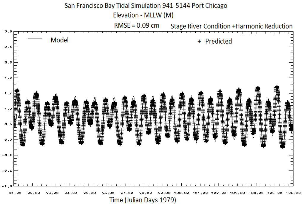
Figure 5.
Comparison of modeled versus predicted water level at Port Chicago with stage boundary condition and 5% harmonic amplitude reduction over the period 1–15 April 1979.
4.2. Extensive Tidal Calibration
For further calibration, the model setup used for the short term tidal experiment was used over an extended 19-month simulation from April 1979 through October 1980. Meteorological forcings were specified by setting the wind speed to zero and the sea level atmospheric pressure to 1013 mb over the entire model domain. A nudging of both salinity and temperature to specified climatological values was used along the open ocean boundary. The nineteen month simulation was completed in 38 segments of approximately 15 days’ duration each, with each segment restarted from the previous segment’s final fields.
In Table 3, simulation segment results for water surface elevation are compared respectively to harmonic predictions in terms of RMS error and Willmott relative error [39], which is given by <(abs(Y-X))2>/<(abs(Y-<X>)+abs(X-<X>))2>, with Y the model prediction and X the observation. Station locations can be found in Figure 6. In addition, model and predicted means are compared with respect to station MLLW. In general, the water level RMS errors do not exceed 15 cm and are consistent from month to month from Port Chicago in Suisun Bay through San Pablo and mid-Bay regions, as well as in the offshore and southern regions of San Francisco Bay. At Coyote Creek, at the southern end of South Bay, while the means are in close agreement, the RMS errors range from 13 to 22 cm and often exceed 15 cm. The adjustment of the bottom friction over salt marsh regions undergoing wetting and drying may need further consideration. In Table 4, principal component direction currents at mid layer (k = 10) are compared respectively to harmonic predictions in terms of RMS error and Willmott relative error. In addition, model and predicted mean currents are given. Current amplitude RMS errors are consistent from month to month and are generally less than 35 cm/s. Willmott relative errors are less than 10% except at C-33.
A more formal skill assessment has been performed in two parts. In part one, harmonic analysis was used to compare water level and principal component current strengths for the M2, S2, N2, O1, and K1 tidal constituents. NOS accepted harmonic constants are compared with tidal simulation results in Table 5. Favorable comparisons were obtained for all constituents at all stations. In Table 6, model principal component current strengths are compared with NOS harmonic constants. Again, comparisons are favorable for both amplitude and phase at most stations except at Station C-18 for the M2 amplitude. In part two, model and predicted means, root mean square error, standard deviation of the error, and central frequency (at reference levels of 15 cm for water level and 26 cm/s for current) were considered. In Table 7, water level skill assessment results are given with favorable comparisons exhibited for means and RMSE at all stations with the exception of Coyote Creek, where the water level error exceeded 15 cm 33.9% of the time. In Table 8, principal component current strength skill assessment results are shown with favorable results observed at most stations except again at Station C-18.
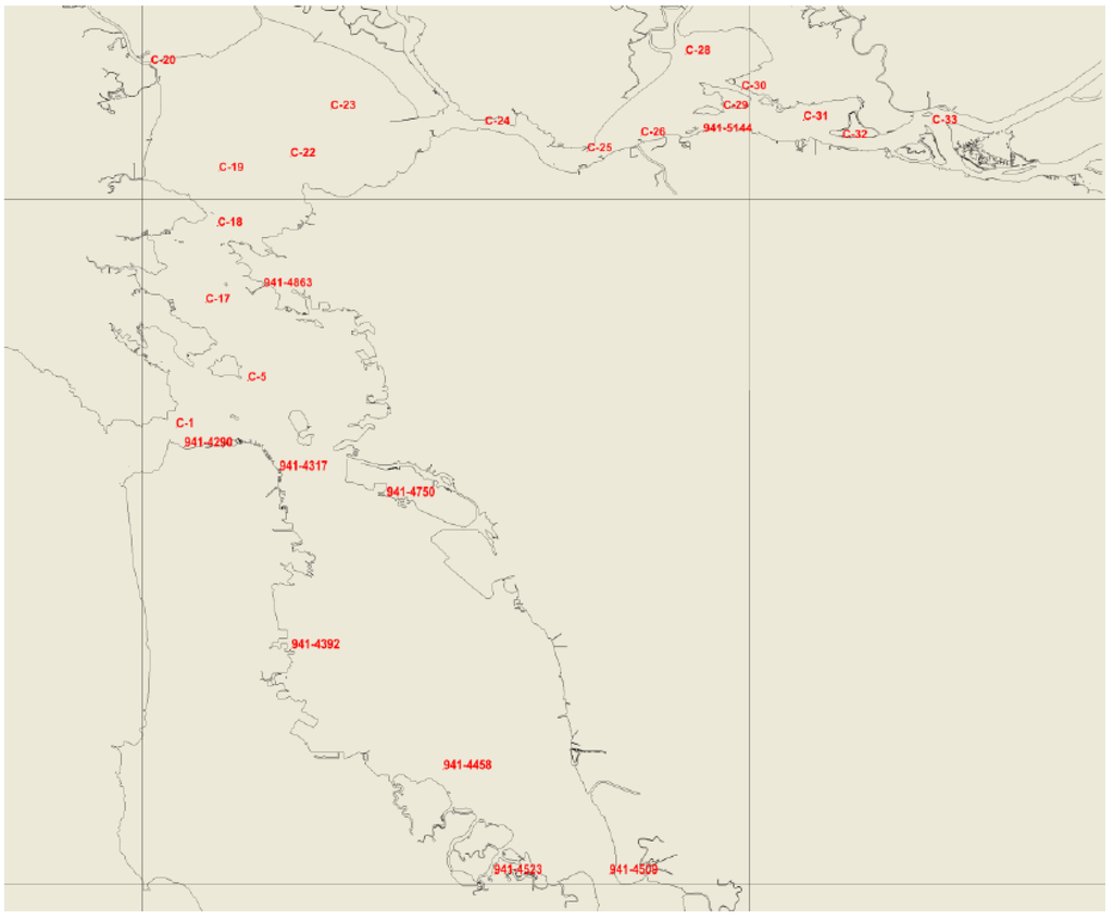
Figure 6.
NOS and USGS Historical Circulation Survey Water Level, Current, Salinity, and Temperature Stations. Note current meters were collocated with conductivity-temperature sensors. Note the location of Point Reyes is shown in Figure 1.
The heat flux algorithm generates no excessive temperatures and produces accurate seasonal heating and cooling [22]. No comparisons with observed salinity are made, since meteorological forcings are not included. However, the simulated salinity gradients are reasonable and a density front is present with the inclusion of the freshwater inflows [22]. The salinity structures through the entrance are in line with climatological values. In the next section, all forcings will be turned on for the hindcast simulation and the model skill assessment will be conducted for further validation.
Table 3.
Water Surface Elevation Tidal Calibration: April 1979–October 1980. For each box, the first column of values corresponds to the first 15 days of the month, with the second column of values denoting the remaining portion of the month. Within each column: Row 1 corresponds to the RMSE in cm. Row 2 corresponds to the Willmott Relative Error in percent. Row 3 corresponds to the model mean in cm with respect to MLLW with Row 4 denoting the predicted water level mean in cm relative to MLLW.
| 1979 | ||||||||||||||||||||||||||||||||
|---|---|---|---|---|---|---|---|---|---|---|---|---|---|---|---|---|---|---|---|---|---|---|---|---|---|---|---|---|---|---|---|---|
| Apr | May | Jun | Jul | Aug | Sep | Oct | Nov | Dec | ||||||||||||||||||||||||
| Alameda 941-4750 | 9 | 6 | 5 | 6 | 5 | 6 | 6 | 6 | 7 | 6 | 8 | 7 | 7 | 7 | 6 | 6 | 6 | 5 | ||||||||||||||
| 1 | 0 | 0 | 0 | 0 | 0 | 0 | 0 | 0 | 0 | 8 | 0 | 0 | 0 | 0 | 0 | 0 | 0 | |||||||||||||||
| 101 | 101 | 100 | 101 | 102 | 104 | 107 | 110 | 112 | 113 | 113 | 112 | 111 | 109 | 108 | 108 | 107 | 108 | |||||||||||||||
| 102 | 100 | 98 | 99 | 100 | 102 | 104 | 107 | 109 | 109 | 109 | 108 | 107 | 105 | 104 | 105 | 105 | 106 | |||||||||||||||
| Dumbarton Bridge 941-4509 | 13 | 11 | 9 | 10 | 10 | 10 | 11 | 9 | 12 | 8 | 12 | 8 | 11 | 8 | 10 | 8 | 9 | 8 | ||||||||||||||
| 1 | 1 | 0 | 0 | 0 | 0 | 0 | 0 | 1 | 0 | 1 | 0 | 0 | 0 | 0 | 0 | 0 | 0 | |||||||||||||||
| 135 | 135 | 134 | 135 | 136 | 139 | 142 | 144 | 147 | 147 | 148 | 146 | 145 | 143 | 142 | 142 | 141 | 142 | |||||||||||||||
| 135 | 132 | 132 | 132 | 134 | 136 | 139 | 141 | 144 | 144 | 144 | 143 | 141 | 140 | 139 | 139 | 140 | 141 | |||||||||||||||
| Oyster Point Marina 941-4392 | 10 | 7 | 4 | 7 | 7 | 7 | 8 | 7 | 9 | 7 | 9 | 8 | 8 | 8 | 7 | 8 | 6 | 8 | ||||||||||||||
| 1 | 0 | 0 | 0 | 0 | 0 | 0 | 0 | 0 | 0 | 0 | 0 | 0 | 0 | 0 | 0 | 0 | 0 | |||||||||||||||
| 111 | 111 | 110 | 111 | 112 | 114 | 117 | 120 | 123 | 123 | 123 | 122 | 121 | 119 | 118 | 118 | 117 | 118 | |||||||||||||||
| 111 | 109 | 108 | 108 | 109 | 112 | 115 | 117 | 120 | 120 | 120 | 119 | 117 | 116 | 115 | 115 | 115 | 116 | |||||||||||||||
| Port Chicago 941-5144 | 9 | 7 | 7 | 7 | 7 | 7 | 8 | 7 | 8 | 7 | 7 | 7 | 6 | 7 | 6 | 7 | 6 | 8 | ||||||||||||||
| 1 | 0 | 1 | 1 | 1 | 1 | 1 | 1 | 1 | 1 | 1 | 1 | 0 | 1 | 0 | 1 | 1 | 1 | |||||||||||||||
| 76 | 76 | 74 | 74 | 76 | 78 | 81 | 84 | 86 | 85 | 84 | 82 | 79 | 76 | 74 | 74 | 75 | 78 | |||||||||||||||
| 76 | 74 | 72 | 73 | 74 | 77 | 80 | 82 | 84 | 84 | 82 | 79 | 76 | 73 | 72 | 72 | 74 | 77 | |||||||||||||||
| Point Reyes 941-5020 | 7 | 4 | 4 | 4 | 4 | 4 | 5 | 4 | 6 | 3 | 5 | 3 | 5 | 3 | 4 | 4 | 4 | 5 | ||||||||||||||
| 1 | 0 | 0 | 0 | 0 | 0 | 0 | 0 | 0 | 0 | 0 | 0 | 0 | 0 | 0 | 0 | 0 | 0 | |||||||||||||||
| 89 | 88 | 88 | 88 | 90 | 93 | 95 | 98 | 100 | 101 | 102 | 101 | 100 | 99 | 98 | 98 | 98 | 98 | |||||||||||||||
| 88 | 86 | 86 | 86 | 88 | 90 | 93 | 96 | 99 | 100 | 101 | 100 | 99 | 98 | 97 | 97 | 97 | 97 | |||||||||||||||
| San Francisco 941-4290 | 7 | 4 | 4 | 4 | 4 | 5 | 4 | 5 | 5 | 5 | 5 | 5 | 5 | 5 | 4 | 5 | 3 | 5 | ||||||||||||||
| 1 | 0 | 0 | 0 | 0 | 0 | 0 | 0 | 0 | 0 | 0 | 0 | 0 | 0 | 0 | 0 | 0 | 0 | |||||||||||||||
| 91 | 89 | 89 | 89 | 90 | 93 | 96 | 99 | 101 | 102 | 102 | 101 | 100 | 99 | 98 | 97 | 97 | 97 | |||||||||||||||
| 91 | 89 | 88 | 88 | 89 | 92 | 94 | 97 | 99 | 100 | 100 | 99 | 97 | 96 | 95 | 95 | 95 | 97 | |||||||||||||||
| San Mateo Bridge 941-4458 | 10 | 8 | 6 | 7 | 7 | 7 | 8 | 6 | 9 | 6 | 9 | 6 | 5 | 6 | 7 | 6 | 7 | 5 | ||||||||||||||
| 1 | 0 | 0 | 0 | 0 | 0 | 0 | 0 | 0 | 0 | 0 | 0 | 0 | 0 | 0 | 0 | 0 | 0 | |||||||||||||||
| 122 | 122 | 121 | 121 | 122 | 125 | 128 | 130 | 133 | 133 | 134 | 133 | 131 | 130 | 128 | 128 | 128 | 128 | |||||||||||||||
| 121 | 119 | 118 | 118 | 119 | 122 | 125 | 127 | 130 | 130 | 130 | 129 | 127 | 126 | 125 | 125 | 126 | 127 | |||||||||||||||
| Coyote Creek 941-4575 | 17 | 20 | 15 | 19 | 17 | 19 | 17 | 16 | 17 | 14 | 16 | 14 | 16 | 15 | 17 | 16 | 18 | 16 | ||||||||||||||
| 1 | 1 | 1 | 1 | 1 | 1 | 1 | 1 | 1 | 1 | 1 | 1 | 1 | 1 | 1 | 1 | 1 | 1 | |||||||||||||||
| 147 | 148 | 146 | 148 | 148 | 151 | 154 | 156 | 159 | 159 | 160 | 158 | 157 | 155 | 154 | 154 | 153 | 154 | |||||||||||||||
| 146 | 144 | 142 | 143 | 144 | 147 | 150 | 152 | 154 | 155 | 155 | 154 | 152 | 151 | 150 | 150 | 150 | 151 | |||||||||||||||
| 1980 | ||||||||||||||||||||||||||||||||
| Jan | Feb | Mar | Apr | May | Jun | Jul | Aug | Sep | Oct | |||||||||||||||||||||||
| Alameda 941-4750 | 6 | 5 | 6 | 5 | 6 | 5 | 7 | 4 | 7 | 4 | 7 | 5 | 7 | 5 | 7 | 6 | 7 | 7 | 6 | 7 | ||||||||||||
| 0 | 0 | 0 | 0 | 0 | 0 | 0 | 0 | 0 | 0 | 0 | 0 | 0 | 0 | 0 | 0 | 0 | 0 | 0 | 0 | |||||||||||||
| 108 | 109 | 109 | 108 | 106 | 104 | 102 | 101 | 100 | 100 | 98 | 105 | 107 | 110 | 112 | 113 | 113 | 112 | 110 | 110 | |||||||||||||
| 108 | 109 | 109 | 108 | 106 | 104 | 101 | 100 | 98 | 99 | 100 | 102 | 104 | 107 | 109 | 109 | 109 | 108 | 107 | 106 | |||||||||||||
| Dumbarton Bridge 941-4509 | 9 | 10 | 9 | 9 | 10 | 9 | 11 | 8 | 12 | 8 | 13 | 8 | 11 | 9 | 9 | 10 | 8 | 11 | 7 | 11 | ||||||||||||
| 0 | 0 | 0 | 0 | 0 | 0 | 1 | 0 | 1 | 0 | 1 | 0 | 0 | 0 | 0 | 0 | 0 | 0 | 0 | 1 | |||||||||||||
| 142 | 143 | 143 | 142 | 141 | 138 | 137 | 135 | 134 | 134 | 133 | 139 | 142 | 144 | 146 | 147 | 147 | 147 | 144 | 144 | |||||||||||||
| 142 | 143 | 143 | 142 | 140 | 137 | 135 | 133 | 132 | 132 | 133 | 136 | 139 | 141 | 144 | 145 | 144 | 143 | 141 | 141 | |||||||||||||
| Oyster Point Marina 941-4392 | 7 | 8 | 7 | 8 | 7 | 6 | 8 | 5 | 8 | 6 | 8 | 6 | 8 | 6 | 8 | 7 | 8 | 8 | 7 | 8 | ||||||||||||
| 0 | 0 | 0 | 0 | 0 | 0 | 0 | 0 | 0 | 0 | 0 | 0 | 0 | 0 | 0 | 0 | 0 | 0 | 0 | 0 | |||||||||||||
| 118 | 119 | 119 | 118 | 117 | 115 | 113 | 111 | 110 | 110 | 108 | 115 | 117 | 120 | 122 | 123 | 123 | 122 | 120 | 120 | |||||||||||||
| 118 | 118 | 118 | 118 | 116 | 113 | 111 | 109 | 107 | 108 | 109 | 112 | 114 | 117 | 119 | 120 | 120 | 119 | 117 | 116 | |||||||||||||
| Port Chicago 941-5144 | 7 | 8 | 6 | 8 | 6 | 7 | 6 | 7 | 7 | 7 | 7 | 7 | 8 | 7 | 8 | 7 | 7 | 7 | 7 | 6 | ||||||||||||
| 1 | 1 | 1 | 1 | 1 | 1 | 1 | 1 | 1 | 1 | 1 | 1 | 1 | 1 | 1 | 1 | 1 | 1 | 1 | 1 | |||||||||||||
| 81 | 84 | 84 | 84 | 82 | 80 | 77 | 75 | 74 | 74 | 75 | 79 | 82 | 84 | 86 | 86 | 84 | 82 | 78 | 76 | |||||||||||||
| 80 | 83 | 84 | 84 | 82 | 79 | 76 | 74 | 72 | 73 | 74 | 77 | 80 | 82 | 84 | 84 | 82 | 79 | 76 | 74 | |||||||||||||
| Point Reyes 941-5020 | 3 | 6 | 4 | 6 | 4 | 5 | 5 | 5 | 5 | 4 | 6 | 4 | 4 | 4 | 4 | 4 | 4 | 5 | 4 | 5 | ||||||||||||
| 0 | 0 | 0 | 0 | 0 | 0 | 0 | 0 | 0 | 0 | 0 | 0 | 0 | 0 | 0 | 0 | 0 | 0 | 0 | 0 | |||||||||||||
| 98 | 98 | 98 | 96 | 95 | 92 | 90 | 89 | 88 | 88 | 86 | 93 | 95 | 98 | 100 | 101 | 102 | 101 | 100 | 99 | |||||||||||||
| 98 | 97 | 97 | 95 | 93 | 90 | 88 | 86 | 86 | 86 | 88 | 91 | 93 | 96 | 99 | 100 | 100 | 100 | 99 | 99 | |||||||||||||
| San Francisco 941-4290 | 3 | 5 | 3 | 6 | 3 | 5 | 4 | 4 | 4 | 4 | 6 | 3 | 5 | 4 | 6 | 4 | 6 | 5 | 6 | 5 | ||||||||||||
| 0 | 0 | 0 | 0 | 0 | 0 | 0 | 0 | 0 | 0 | 0 | 0 | 0 | 0 | 0 | 0 | 0 | 0 | 0 | 0 | |||||||||||||
| 98 | 98 | 98 | 97 | 96 | 93 | 91 | 89 | 88 | 89 | 86 | 94 | 96 | 98 | 101 | 102 | 102 | 101 | 100 | 99 | |||||||||||||
| 98 | 98 | 99 | 98 | 96 | 93 | 91 | 89 | 88 | 88 | 89 | 92 | 94 | 97 | 99 | 100 | 100 | 99 | 97 | 96 | |||||||||||||
| San Mateo Bridge 941-4458 | 6 | 7 | 7 | 7 | 7 | 6 | 8 | 5 | 9 | 5 | 9 | 6 | 8 | 6 | 7 | 7 | 6 | 8 | 6 | 9 | ||||||||||||
| 0 | 0 | 0 | 0 | 0 | 0 | 0 | 0 | 0 | 0 | 0 | 0 | 0 | 0 | 0 | 0 | 0 | 0 | 0 | 0 | |||||||||||||
| 129 | 129 | 129 | 129 | 127 | 125 | 123 | 121 | 121 | 121 | 119 | 125 | 128 | 130 | 133 | 134 | 133 | 133 | 131 | 130 | |||||||||||||
| 128 | 129 | 129 | 128 | 126 | 123 | 121 | 119 | 118 | 118 | 119 | 122 | 125 | 127 | 130 | 131 | 130 | 129 | 127 | 127 | |||||||||||||
| Coyote Creek 941-4575 | 17 | 18 | 17 | 15 | 17 | 14 | 19 | 14 | 21 | 15 | 22 | 15 | 20 | 15 | 16 | 15 | 14 | 16 | 13 | 17 | ||||||||||||
| 1 | 1 | 1 | 1 | 1 | 1 | 1 | 1 | 2 | 1 | 2 | 1 | 1 | 1 | 1 | 1 | 1 | 1 | 1 | 1 | |||||||||||||
| 154 | 155 | 155 | 154 | 153 | 151 | 149 | 147 | 146 | 147 | 145 | 151 | 154 | 156 | 158 | 160 | 159 | 159 | 156 | 156 | |||||||||||||
| 153 | 153 | 153 | 153 | 151 | 148 | 145 | 144 | 142 | 143 | 144 | 147 | 150 | 152 | 154 | 155 | 154 | 154 | 152 | 151 | |||||||||||||
Table 4.
Principal Current Direction Mid-Level Current Speed Tidal Calibration: April 1979–October 1980. For each box, the first column of values corresponds to the first 15 days of the month, with the second column of values denoting the remaining portion. Within each column: Row 1 corresponds to the RMSE in cm/s. Row 2 corresponds to the Willmott Relative Error in percent. Row 3 corresponds to the model mean in cm/s. Note the predicted mean current speed is zero.
| Station | Apr 1979 | May 1979 | Sep 1980 | Oct 1980 | Station | Apr 1979 | May 1979 | Sep 1980 | Oct 1980 | ||||||||
|---|---|---|---|---|---|---|---|---|---|---|---|---|---|---|---|---|---|
| C-1 | 44 | 51 | 48 | 49 | 39 | 52 | 38 | 51 | C-24 | 30 | 38 | 35 | 36 | 29 | 39 | 25 | 36 |
| 9 | 9 | 10 | 8 | 6 | 9 | 6 | 8 | 9 | 12 | 11 | 11 | 8 | 11 | 6 | 9 | ||
| 8 | 10 | 8 | 9 | 8 | 8 | 7 | 7 | −10 | −12 | −12 | −12 | −11 | −11 | −9 | −8 | ||
| C-5 | 25 | 31 | 27 | 30 | 25 | 29 | 24 | 28 | C-25 | 15 | 21 | 20 | 22 | 20 | 23 | 17 | 20 |
| 10 | 11 | 11 | 12 | 10 | 11 | 9 | 10 | 3 | 5 | 6 | 6 | 6 | 7 | 5 | 5 | ||
| 11 | 12 | 11 | 11 | 10 | 10 | 9 | 7 | 6 | 11 | 12 | 13 | 14 | 14 | 11 | 10 | ||
| C-17 | 14 | 14 | 14 | 13 | 12 | 13 | 9 | 13 | C-26 | 15 | 19 | 16 | 19 | 14 | 22 | 14 | 22 |
| 4 | 3 | 4 | 3 | 2 | 2 | 2 | 2 | 3 | 3 | 3 | 4 | 2 | 5 | 2 | 5 | ||
| 9 | 6 | 8 | 5 | 5 | 4 | 3 | 2 | −4 | −1 | −1 | 1 | 1 | 3 | 2 | 3 | ||
| C-18 | 25 | 26 | 24 | 24 | 20 | 22 | 16 | 20 | C-28 | 9 | 10 | 9 | 11 | 10 | 9 | 10 | 10 |
| 5 | 4 | 5 | 4 | 3 | 3 | 2 | 3 | 9 | 7 | 8 | 9 | 10 | 7 | 10 | 8 | ||
| 16 | 15 | 15 | 13 | 11 | 12 | 11 | 10 | 0 | 1 | 1 | 1 | 1 | 2 | 2 | 2 | ||
| C-19 | 9 | 11 | 10 | 11 | 8 | 10 | 7 | 10 | C-29 | 12 | 14 | 13 | 15 | 11 | 16 | 10 | 17 |
| 3 | 3 | 3 | 3 | 2 | 2 | 2 | 3 | 3 | 4 | 4 | 4 | 3 | 5 | 3 | 5 | ||
| 3 | 4 | 3 | 4 | 4 | 4 | 3 | 4 | 1 | −1 | 0 | −2 | −3 | −4 | −4 | −5 | ||
| C-20 | 17 | 20 | 18 | 19 | 16 | 21 | 16 | 21 | C-30 | 11 | 11 | 11 | 12 | 13 | 15 | 13 | 15 |
| 12 | 12 | 13 | 12 | 10 | 13 | 11 | 14 | 3 | 2 | 2 | 3 | 4 | 4 | 4 | 4 | ||
| 0 | 0 | 1 | 1 | 0 | 0 | 1 | 1 | 2 | −1 | 0 | −2 | −3 | −5 | −5 | −6 | ||
| C-22 | 13 | 10 | 11 | 10 | 11 | 9 | 10 | 9 | C-31 | 8 | 10 | 9 | 11 | 7 | 11 | 7 | 12 |
| 3 | 1 | 2 | 1 | 2 | 1 | 2 | 1 | 4 | 6 | 5 | 6 | 3 | 6 | 4 | 8 | ||
| 6 | 4 | 6 | 4 | 4 | 3 | 2 | 2 | 1 | 3 | 2 | 3 | 3 | 3 | 2 | 2 | ||
| C-23 | 5 | 5 | 5 | 5 | 4 | 5 | 4 | 5 | C-33 | 24 | 30 | 26 | 29 | 24 | 32 | 25 | 33 |
| 2 | 2 | 2 | 2 | 2 | 2 | 2 | 2 | 8 | 20 | 19 | 20 | 16 | 24 | 19 | 24 | ||
| 1 | 2 | 2 | 2 | 1 | 1 | 1 | 2 | 0 | −2 | −1 | −2 | −4 | −7 | −8 | −9 | ||
Table 5.
Harmonic Analysis of 19-month tidal simulation water level comparison to NOS accepted tidal constituents. Accepted constituent values of amplitudes (m) and phase (degrees) minus model predictions. Note negative amplitude differences denote an under prediction of tidal water level constituent amplitudes, while positive phases denote a lag in tidal water level constituent propagation.
| Station/Constituent | M2 | S2 | N2 | O1 | K1 | |||||
|---|---|---|---|---|---|---|---|---|---|---|
| 941-5020 Point Reyes, CA | −0.023 | 0.3 | −0.004 | 0.0 | −0.007 | −0.4 | −0.012 | −1.3 | −0.023 | 1.5 |
| 941-4290 San Francisco, CA | 0.020 | −1.2 | 0.020 | −1.2 | 0.020 | −1.2 | −0.002 | −4.4 | −0.005 | −0.3 |
| 941-4358 Hunters Point, CA | 0.018 | 2.8 | −0.007 | 0.3 | −0.010 | 1.3 | −0.002 | −1.1 | −0.017 | 2.0 |
| 941-4458 San Mateo Bridge, CA | −0.004 | 3.0 | −0.009 | 3.6 | −0.013 | 2.8 | −0.005 | −1.0 | −0.013 | 3.1 |
| 941-4523 Redwood City, CA | −0.005 | 6.6 | −0.007 | 6.9 | −0.014 | 7.4 | −0.004 | 1.1 | −0.022 | 5.5 |
| 941-4509 Dumbarton Bridge, CA | −0.014 | 4.8 | −0.007 | 6.8 | −0.012 | 6.0 | −0.005 | −0.1 | −0.022 | 4.6 |
| 941-4575 Coyote Creek, CA | −0.027 | 8.8 | −0.017 | 9.6 | −0.014 | 8.4 | 0.003 | 4.2 | −0.014 | 8.4 |
| 941-4750 Alameda, CA | 0.025 | 3.3 | −0.002 | 2.0 | −0.005 | 1.8 | −0.001 | −2.2 | −0.004 | 1.9 |
| 941-4863 Richmond, CA | 0.016 | −0.9 | −0.005 | −4.1 | −0.008 | −2.5 | −0.008 | −4.2 | −0.014 | −0.4 |
| 941-5144 Port Chicago, CA | 0.012 | −4.4 | −0.006 | −7.3 | −0.008 | 0.1 | −0.008 | −2.6 | −0.020 | 2.4 |
Table 6.
Harmonic Analysis of 19-month tidal simulation principal current direction current comparison to NOS accepted tidal current constituents. Accepted constituent values of amplitudes (m/s) and phase (degrees) minus model predictions. Note negative amplitude differences denote an under prediction of tidal current constituent amplitudes, while positive phases denote a lag in tidal current constituent propagation. Along with station id measurement, depths are given in parenthesis with observed/model principal component directions given following the depth information.
| Station/Constituent | M2 | S2 | N2 | O1 | K1 | |||||
|---|---|---|---|---|---|---|---|---|---|---|
| C-1 (7.62m) 83/75 | −0.209 | −12.3 | −0.014 | 3.8 | −0.050 | −38.3 | −0.061 | −17.8 | −0.101 | −3.8 |
| C-5 (1.83m) 3/30 | −0.148 | −13.3 | −0.114 | −11.9 | −0.035 | −33.4 | −0.056 | −13.9 | −0.127 | −6.3 |
| C-18 (15.24m) 34/20 | 0.414 | 2.7 | 0.058 | −2.9 | 0.059 | −17.3 | 0.060 | −5.2 | 0.126 | −4.6 |
| C-20 (0.92m) 97/104 | −0.226 | −1.7 | −0.064 | −0.4 | −0.047 | −12.3 | −0.020 | −1.7 | −0.062 | 0.5 |
| C-22 (1.52m) 53/53 | −0.147 | −12.5 | −0.042 | −5.4 | −0.027 | −31.1 | −0.031 | −2.5 | −0.066 | −1.8 |
| C-25 (1.52m) 53/58 | −0.126 | −7.5 | −0.071 | −2.2 | −0.030 | −32.9 | −0.002 | 12.6 | −0.053 | 13.5 |
| C-26 (1.83m) 61/64 | −0.271 | −13.2 | −0.064 | 4.8 | −0.068 | −45.0 | −0.053 | −4.2 | −0.070 | −2.8 |
Table 7.
Nineteen-month Tidal Simulation Water Level Skill Assessment Results. Results are with respect to MSL. RMSE is root mean square error, SD is standard deviation of the error; e.g., model minus observation, and CF is central frequency of the errors with respect to a reference level of 0.15 m.
| Station/Skill Parameter | Model Mean (m) | Prediction Mean (m) | RMSE (m) | SD (m) | CF (%) |
|---|---|---|---|---|---|
| 941-5020 Point Reyes, CA | −0.004 | −0.004 | 0.043 | 0.043 | 99.9 |
| 941-4290 San Francisco, CA | −0.003 | −0.003 | 0.045 | 0.045 | 99.9 |
| 941-4305 North Point Pier 41, CA | −0.003 | −0.003 | 0.047 | 0.047 | 99.9 |
| 941-4358 Hunters Point, CA | −0.003 | −0.003 | 0.061 | 0.061 | 99.0 |
| 941-4458 San Mateo Bridge, CA | −0.003 | −0.003 | 0.069 | 0.069 | 97.1 |
| 941-4523 Redwood City, CA | −0.003 | −0.003 | 0.107 | 0.107 | 85.4 |
| 941-4509 Dumbarton Bridge, CA | −0.003 | −0.003 | 0.100 | 0.100 | 88.0 |
| 941-4575 Coyote Creek, CA | −0.002 | −0.003 | 0.168 | 0.168 | 66.1 |
| 941-4750 Alameda, CA | −0.003 | −0.003 | 0.060 | 0.060 | 98.9 |
| 941-4863 Richmond, CA | −0.004 | −0.004 | 0.049 | 0.049 | 99.9 |
| 941-5144 Port Chicago, CA | −0.002 | −0.002 | 0.069 | 0.069 | 97.4 |
Table 8.
Nineteen-month Tidal Simulation Principal Component Direction Current Strength Skill Assessment Results. Note measurement depth given in parenthesis followed by observed/model principal current direction. RMSE is root mean square error, SD is standard deviation of the error; e.g., model minus observation, and CF is central frequency of the errors with respect to a reference level of 0.26 m/s.
| Station/Skill Parameter | Model Mean (m/s) | Prediction Mean (m/s) | RMSE (m/s) | SD (m/s) | CF (%) |
|---|---|---|---|---|---|
| C-1 (7.62m) 83/75 | 0.629 | 0.698 | 0.249 | 0.239 | 68.8 |
| C-5 (1.83m) 3/30 | 0.332 | 0.426 | 0.208 | 0.185 | 81.2 |
| C-18 (15.24m) 34/20 | 0.716 | 0.460 | 0.339 | 0.222 | 46.5 |
| C-20 (0.92m) 97/104 | 0.161 | 0.310 | 0.194 | 0.125 | 83.7 |
| C-22 (1.52m) 53/53 | 0.349 | 0.445 | 0.166 | 0.136 | 88.3 |
| C-25 (1.52m) 53/58 | 0.361 | 0.420 | 0.165 | 0.154 | 88.1 |
| C-26 (1.83m) 61/64 | 0.367 | 0.538 | 0.253 | 0.185 | 66.7 |
5. Hindcast Validation
An extended 19-month hindcast model validation was performed with complete meteorological forcings. The details of the model setup can be found in Section 3. During the simulation period, RMS wind speed errors are less than 5 m/s with direction RMS errors order 50 degrees. For sea level atmospheric pressure, the RMS errors are near 2 mb. For the offshore temperature and salinity, a zero gradient boundary condition is used. Since the meteorological forcings are at 3 h intervals, the effect of the sea breeze may not be completely captured.
The results are presented in 15 day increments in Table 9 for water levels. There are fewer stations available with measured data for comparison than for the tidal calibration. In addition, there are gauge datum issues at several water level stations. Generally, the water level RMS errors do not exceed 15 cm and are consistent from month to month in almost all regions. At Point Reyes, there are issues with the data, which cause errors in the subtidal water level forcings for several months indicated as blanks.
As shown in Table 10, current amplitude RMS errors are consistent throughout the period and are generally less than 35 cm/s. The salinity response is summarized in Table 11. Generally, the model salinity was in agreement with the observations at most of the stations. However, it was overestimated in the northern portion of San Pablo Bay and throughout Suisun Bay. This is believed to be due to the fact that the river subtidal water levels were not included since no measured river stage data were available. As a result, the model results could not correctly reflect the freshwater runoff during the high flow months when substantial river subtidal levels were present. This in effect, limited the amount of freshwater entering the Bay through the Delta. The temperature response is summarized in Table 12 and exhibited a normal seasonal response, but in October 1980 there was some evidence of overheating by about 2 °C in Suisun Bay.
In addition to the validation in terms of RMS errors, the NOS skill assessment criteria [40,41] are also applied to the hindcast. We show in Table 13 the results at some of the major water level stations. Additional model skill assessment results for currents, salinity, and temperature are given in [22]. Generally, the skill assessment indicates that most water-level related statistical parameters pass the NOS skill assessment criteria for different scenarios, and that amplitudes and epochs of major harmonic constituents such as M2, S2, N2, K2, K1, O1, P1, and Q1 from the tide-only scenario simulation are very close to the observed values at almost all stations.
Most of CF (Central Frequency), NOF (Negative Outlier Frequency), POF (Positive Outlier Frequency), MDNO (Maximum Duration of Positive Outliers), and MDPO (Maximum Duration of Positive Outliers) either pass or are close to the criteria at the Bay current stations for not only the tide-only scenario but also the hindcast scenario, since tidal current dominates the signal in San Francisco Bay region. See Schmalz [22] for more complete definitions of the skill assessment parameters.
The tidal and hindcast simulations indicate that the SFBOFS runs robustly and that the results are in acceptable agreement with the measurements. The model package was therefore loaded into the COMF-HPC on NCEP’s high performance computers to perform semi-operational nowcast/forecasts.
Table 9.
Water Surface Elevation Hindcast Validation: April 1979–October 1980. For each box, the first column of values corresponds to the first 15 days of the month, with the second column denoting the remaining portion of the month. Within each column: Row 1 corresponds to the RMSE in cm. Row 2 corresponds to the Willmott Relative Error in percent. Row 3 corresponds to the model mean in cm relative to MLLW. Row 4 denoting the observed water level mean in cm with respect to MLLW.
| 1979 | |||||||||||||||||||||||||||||||||
|---|---|---|---|---|---|---|---|---|---|---|---|---|---|---|---|---|---|---|---|---|---|---|---|---|---|---|---|---|---|---|---|---|---|
| Apr | May | Jun | Jul | Aug | Sep | Oct | Nov | Dec | |||||||||||||||||||||||||
| Alameda 941-4750 | 1 | 9 | 7 | 6 | 8 | 6 | 7 | ||||||||||||||||||||||||||
| 2 | 1 | 0 | 0 | 0 | 0 | 0 | |||||||||||||||||||||||||||
| 3 | 112 | 108 | 107 | 99 | 103 | 113 | |||||||||||||||||||||||||||
| 4 | 105 | 103 | 104 | 95 | 100 | 111 | |||||||||||||||||||||||||||
| Point Reyes 941-5020 | 1 | 7 | 5 | 4 | 4 | 5 | 4 | 5 | 4 | 4 | 5 | 4 | 5 | ||||||||||||||||||||
| 2 | 1 | 0 | 0 | 0 | 0 | 0 | 0 | 0 | 0 | 0 | 0 | 0 | |||||||||||||||||||||
| 3 | 81 | 82 | 80 | 87 | 87 | 96 | 98 | 96 | 96 | 87 | 91 | 102 | |||||||||||||||||||||
| 4 | 80 | 79 | 78 | 85 | 85 | 94 | 96 | 94 | 95 | 85 | 90 | 102 | |||||||||||||||||||||
| San Francisco 941-4290 | 1 | 5 | 5 | 8 | 8 | 7 | 6 | 3 | 4 | 5 | 6 | ||||||||||||||||||||||
| 2 | 0 | 0 | 0 | 1 | 0 | 0 | 0 | 0 | 0 | 0 | |||||||||||||||||||||||
| 3 | 83 | 88 | 90 | 98 | 99 | 96 | 96 | 88 | 92 | 102 | |||||||||||||||||||||||
| 4 | 79 | 86 | 83 | 91 | 93 | 92 | 96 | 86 | 88 | 100 | |||||||||||||||||||||||
| Pier 22.5 941-4317 | 1 | 10 | 9 | 7 | 7 | 6 | 6 | ||||||||||||||||||||||||||
| 2 | 1 | 1 | 0 | 0 | 0 | 0 | |||||||||||||||||||||||||||
| 3 | 105 | 101 | 101 | 92 | 97 | 107 | |||||||||||||||||||||||||||
| 4 | 96 | 94 | 96 | 86 | 93 | 104 | |||||||||||||||||||||||||||
| San Mateo Bridge 941-4458 | 1 | 9 | 8 | 12 | 12 | 12 | 14 | ||||||||||||||||||||||||||
| 2 | 0 | 0 | 1 | 1 | 1 | 1 | |||||||||||||||||||||||||||
| 3 | 117 | 122 | 127 | 120 | 124 | 133 | |||||||||||||||||||||||||||
| 4 | 110 | 117 | 119 | 111 | 116 | 126 | |||||||||||||||||||||||||||
| 1980 | |||||||||||||||||||||||||||||||||
| Jan | Feb | Mar | Apr | May | Jun | Jul | Aug | Sep | Oct | ||||||||||||||||||||||||
| Alameda 941-4750 | 1 | 6 | 11 | 7 | 13 | 12 | 8 | 7 | 5 | 7 | 4 | 7 | 3 | 6 | 4 | 5 | 6 | 6 | 7 | 6 | 6 | ||||||||||||
| 2 | 0 | 1 | 0 | 1 | 1 | 1 | 0 | 0 | 0 | 0 | 0 | 0 | 0 | 0 | 0 | 0 | 0 | 0 | 0 | 0 | |||||||||||||
| 3 | 117 | 107 | 109 | 126 | 112 | 91 | 94 | 96 | 97 | 95 | 98 | 101 | 99 | 109 | 112 | 109 | 110 | 110 | 109 | 101 | |||||||||||||
| 4 | 118 | 115 | 111 | 134 | 119 | 97 | 95 | 98 | 98 | 96 | 98 | 101 | 97 | 107 | 110 | 105 | 105 | 107 | 107 | 98 | |||||||||||||
| Oyster Point Marina 941-4392 | 1 | 15 | 10 | 13 | 10 | 14 | 8 | 14 | 9 | 10 | 9 | ||||||||||||||||||||||
| 2 | 1 | 1 | 1 | 1 | 1 | 0 | 1 | 0 | 1 | 0 | |||||||||||||||||||||||
| 3 | 104 | 106 | 107 | 106 | 108 | 111 | 110 | 119 | 122 | 119 | |||||||||||||||||||||||
| 4 | 104 | 107 | 106 | 103 | 106 | 108 | 105 | 118 | 121 | 116 | |||||||||||||||||||||||
| Port Chicago 941-5144 | 1 | 13 | 22 | 8 | 32 | 23 | 10 | 11 | 9 | 9 | 9 | 8 | 7 | 9 | 6 | 6 | 7 | 7 | 6 | 6 | 10 | ||||||||||||
| 2 | 2 | 5 | 1 | 11 | 8 | 1 | 2 | 1 | 1 | 1 | 1 | 1 | 1 | 0 | 0 | 1 | 1 | 1 | 1 | 1 | |||||||||||||
| 3 | 84 | 81 | 82 | 90 | 82 | 72 | 71 | 70 | 70 | 70 | 72 | 75 | 76 | 82 | 83 | 82 | 81 | 80 | 77 | 73 | |||||||||||||
| 4 | 92 | 98 | 81 | 120 | 102 | 73 | 66 | 70 | 72 | 71 | 73 | 74 | 70 | 80 | 83 | 78 | 77 | 77 | 76 | 66 | |||||||||||||
| Point Reyes 941-5020 | 1 | 4 | 6 | 4 | 6 | 5 | 5 | 5 | 5 | 5 | 4 | 4 | 4 | 5 | 4 | 4 | 5 | 4 | 5 | 4 | 6 | ||||||||||||
| 2 | 0 | 0 | 0 | 0 | 0 | 0 | 0 | 0 | 0 | 0 | 0 | 0 | 0 | 0 | 0 | 0 | 0 | 0 | 0 | 0 | |||||||||||||
| 3 | 106 | 96 | 98 | 116 | 101 | 78 | 81 | 82 | 83 | 81 | 85 | 88 | 86 | 97 | 99 | 96 | 97 | 97 | 97 | 89 | |||||||||||||
| 4 | 106 | 96 | 87 | 117 | 101 | 77 | 79 | 81 | 82 | 80 | 83 | 87 | 84 | 95 | 98 | 94 | 95 | 96 | 96 | 87 | |||||||||||||
| San Francisco 941-4290 | 1 | 5 | 9 | 5 | 11 | 10 | 8 | 6 | 5 | 6 | 3 | 5 | 3 | 6 | 5 | 5 | 5 | 6 | 5 | 6 | 8 | ||||||||||||
| 2 | 0 | 1 | 0 | 1 | 1 | 1 | 0 | 0 | 0 | 0 | 0 | 0 | 0 | 0 | 0 | 0 | 0 | 0 | 0 | 0 | |||||||||||||
| 3 | 106 | 96 | 99 | 116 | 101 | 80 | 83 | 85 | 85 | 84 | 86 | 90 | 88 | 98 | 100 | 97 | 99 | 98 | 98 | 90 | |||||||||||||
| 4 | 106 | 101 | 99 | 120 | 107 | 83 | 83 | 85 | 86 | 85 | 86 | 89 | 84 | 95 | 99 | 94 | 95 | 96 | 96 | 87 | |||||||||||||
| Pier 22.5 941-4317 | 1 | 5 | 10 | 6 | 12 | 10 | 10 | 7 | 11 | 14 | 12 | ||||||||||||||||||||||
| 2 | 0 | 1 | 0 | 1 | 1 | 1 | 0 | 1 | 1 | 1 | |||||||||||||||||||||||
| 3 | 110 | 101 | 104 | 120 | 106 | 85 | 88 | 90 | 90 | 89 | |||||||||||||||||||||||
| 4 | 112 | 108 | 103 | 125 | 105 | 91 | 88 | 89 | 88 | 92 | |||||||||||||||||||||||
| San Mateo Bridge 941-4458 | 1 | 11 | 13 | 10 | 23 | 14 | 8 | 14 | 11 | ||||||||||||||||||||||||
| 2 | 1 | 1 | 1 | 3 | 1 | 0 | 1 | 1 | |||||||||||||||||||||||||
| 3 | 137 | 129 | 130 | 146 | 115 | 117 | 118 | 117 | |||||||||||||||||||||||||
| 4 | 135 | 134 | 129 | 146 | 110 | 115 | 126 | 126 | |||||||||||||||||||||||||
Table 10.
Current Speed Hindcast Validation: April 1979–October 1980. In each box, the first column of values corresponds to the first 15 days of the month, with the second column of values denoting the remaining portion. For each column: Row 1 corresponds to the RMSE in cm/s. Row 2 corresponds to the Willmott Relative Error in percent. Row 3 corresponds to the model mean in cm/s with Row 4 denoting the observed mean current speed in cm/s. Note n/a denotes not available due to incomplete observations. Along with the station id, the measurement location (in distance above the bottom in meters) is given in parenthesis.
| Station | Row | Apr 1979 | May 1979 | Sep 1980 | Oct 1980 | Station | Row | Apr 1979 | May 1979 | Sep 1980 | Oct 1980 | |||||||
|---|---|---|---|---|---|---|---|---|---|---|---|---|---|---|---|---|---|---|
| C-1 (76) | 1 | 15 | 15 | C-19 (1) | 1 | 10 | n/a | 6 | 12 | 9 | n/a | |||||||
| 2 | 4 | 8 | 2 | 25 | n/a | 5 | 14 | 12 | n/a | |||||||||
| 3 | 67 | 73 | 3 | 22 | 26 | 33 | 34 | 32 | 34 | |||||||||
| 4 | 77 | 50 | 4 | 23 | n/a | 28 | 29 | 25 | n/a | |||||||||
| C-1 (91) | 1 | 38 | n/a | C-20 (1) | 1 | 17 | n/a | |||||||||||
| 2 | 26 | n/a | 2 | 35 | n/a | |||||||||||||
| 3 | 63 | 75 | 3 | 15 | 17 | |||||||||||||
| 4 | 80 | n/a | 4 | 27 | n/a | |||||||||||||
| C-5 (2) | 1 | 30 | n/a | C-22 (2) | 1 | 11 | n/a | 10 | 11 | |||||||||
| 2 | 50 | n/a | 2 | 14 | n/a | 9 | 6 | |||||||||||
| 3 | 34 | 39 | 3 | 33 | 38 | 40 | 42 | |||||||||||
| 4 | 29 | n/a | 4 | 29 | n/a | 36 | 39 | |||||||||||
| C-5 (8) | 1 | 33 | n/a | C-23 (1) | 1 | 6 | n/a | n/a | 6 | 5 | 2 | |||||||
| 2 | 42 | n/a | 2 | 29 | n/a | n/a | 27 | 23 | 8 | |||||||||
| 3 | 46 | 52 | 3 | 14 | 16 | 16 | 17 | 16 | 17 | |||||||||
| 4 | 34 | n/a | 4 | 16 | n/a | n/a | 18 | 17 | 12 | |||||||||
| C-5 (25) | 1 | 26 | n/a | C-24 (2) | 1 | 21 | 19 | n/a | 12 | 11 | n/a | |||||||
| 2 | 34 | n/a | 2 | 27 | 23 | n/a | 10 | 11 | n/a | |||||||||
| 3 | 43 | 51 | 3 | 15 | 40 | 41 | 42 | 40 | 42 | |||||||||
| 4 | 35 | n/a | 4 | 14 | 32 | n/a | 44 | 37 | n/a | |||||||||
| C-18 (9) | 1 | 22 | 17 | n/a | 24 | 20 | 19 | C-25 (2) | 1 | 15 | 13 | |||||||
| 2 | 13 | 8 | n/a | 14 | 12 | 12 | 2 | 15 | 12 | |||||||||
| 3 | 60 | 65 | 57 | 59 | 54 | 59 | 3 | 37 | 40 | |||||||||
| 4 | 68 | 63 | n/a | 74 | 63 | 52 | 4 | 41 | 42 | |||||||||
| C-18 (15) | 1 | 21 | 19 | 17 | n/a | n/a | 20 | 18 | 18 | C-26 (2) | 1 | 14 | 22 | n/a | 17 | |||
| 2 | 8 | 6 | 7 | n/a | n/a | 7 | 7 | 9 | 2 | 14 | 25 | n/a | 22 | |||||
| 3 | 68 | 76 | 68 | 75 | 70 | 71 | 67 | 72 | 3 | 38 | 42 | 39 | 40 | |||||
| 4 | 75 | 74 | 55 | n/a | n/a | 83 | 71 | 55 | 4 | 36 | 26 | n/a | 36 | |||||
Table 11.
Salinity Hindcast Validation: April 1979–October 1980. In each row box, the first column of values entry corresponds to the first 15 days of the month, with the second column denoting the remaining portion. Within each column: Row 1 corresponds to the RMSE in PSU. Row 2 corresponds to the Willmott Relative Error in percent. Row 3 corresponds to the model mean in PSU with Row 4 denoting the observed salinity mean in PSU. Note n/a denotes not available due to incomplete observations. Along with the station id, the measurement location (in distance above the bottom in meters) is given in parenthesis.
| Station | Row | Apr 1979 | May 1979 | Sep 1980 | Oct 1980 | Station | Row | Apr 1979 | May 1979 | Sep 1980 | Oct 1980 | |||||||
|---|---|---|---|---|---|---|---|---|---|---|---|---|---|---|---|---|---|---|
| C-1 (46) | 1 | 2 | 3 | n/a | 2 | 1 | n/a | C-19 (1) | 1 | 2 | n/a | 3 | n/a | |||||
| 2 | 41 | 56 | n/a | 58 | 55 | n/a | 2 | 15 | n/a | 0 | n/a | |||||||
| 3 | 30 | 29 | 30 | 30 | 31 | 31 | 3 | 16 | 15 | 23 | 24 | |||||||
| 4 | 31 | 32 | n/a | 32 | 32 | n/a | 4 | 18 | n/a | n/a | n/a | |||||||
| C-1 (91,76) | 1 | 3 | 4 | C-20 (1) | 1 | 14 | n/a | |||||||||||
| 2 | 46 | 61 | 2 | 1 | n/a | |||||||||||||
| 3 | 28 | 27 | 3 | 17 | 13 | |||||||||||||
| 4 | 30 | 31 | 4 | n/a | n/a | |||||||||||||
| C-5 (2) | 1 | 1 | n/a | C-22 (2) | 1 | 3 | n/a | 2 | 1 | |||||||||
| 2 | 37 | n/a | 2 | 31 | n/a | 61 | 15 | |||||||||||
| 3 | 29 | 28 | 3 | 18 | 17 | 24 | 25 | |||||||||||
| 4 | 30 | n/a | 4 | 22 | n/a | 27 | 25 | |||||||||||
| C-5 (8) | 1 | 1 | n/a | C-23 (1) | 1 | n/a | 2 | 3 | 4 | |||||||||
| 2 | 35 | n/a | 2 | n/a | 86 | 71 | 89 | |||||||||||
| 3 | 29 | 28 | 3 | 22 | 23 | 24 | 23 | |||||||||||
| 4 | 29 | n/a | 4 | n/a | 21 | 21 | 19 | |||||||||||
| C-5 (25)MB | 1 | 2 | n/a | C-24 (2,6) | 1 | 10 | 10 | 9 | n/a | n/a | 3 | 3 | n/a | |||||
| 2 | 21 | n/a | 2 | 57 | 60 | 55 | n/a | n/a | 52 | 46 | n/a | |||||||
| 3 | 28 | 27 | 3 | 6 | 6 | 7 | 13 | 22 | 22 | 23 | 22 | |||||||
| 4 | 28 | n/a | 4 | 4 | 13 | n/a | n/a | n/a | 20 | 20 | n/a | |||||||
| C-16 (8) | 1 | 3 | 4 | C-25 (2) | 1 | 18 | n/a | |||||||||||
| 2 | 72 | 59 | 2 | 1 | n/a | |||||||||||||
| 3 | 29 | 29 | 3 | 2 | 2 | |||||||||||||
| 4 | 32 | 32 | 4 | n/a | n/a | |||||||||||||
| C-16 (17) | 1 | 3 | 2 | C-26(2) | 1 | n/a | 10 | |||||||||||
| 2 | 65 | 43 | 2 | n/a | 65 | |||||||||||||
| 3 | 29 | 29 | 3 | 22 | 22 | |||||||||||||
| 4 | 31 | 31 | 4 | n/a | 13 | |||||||||||||
Table 12.
Temperature Hindcast Validation: April 1979–October 1980. In each box month, the first column values correspond to the first 15 days of the month, with the second column of values denoting the remaining portion. Within each column: Row 1 corresponds to the RMSE in °C. Row 2 corresponds to the Willmott Relative Error in percent. Row 3 corresponds to the model mean in °C with Row 4 denoting the observed temperature mean in °C. Note n/a denotes not available due to incomplete observations. Along with the station id, the measurement location (in distance above the bottom in meters) is given in parenthesis.
| Station | Row | Apr 1979 | May 1979 | Sep 1980 | Oct 1980 | Station | Row | Apr 1979 | May 1979 | Sep 1980 | Oct 1980 | |||||||||
|---|---|---|---|---|---|---|---|---|---|---|---|---|---|---|---|---|---|---|---|---|
| C-1 (46,76) | 1 | 1 | 1 | 2 | 1 | C-19 (1) | 1 | 3 | 2 | |||||||||||
| 2 | 57 | 58 | 66 | 46 | 2 | 0 | 59 | |||||||||||||
| 3 | 13 | 13 | 17 | 16 | 3 | 21 | 20 | |||||||||||||
| 4 | 12 | 12 | 15 | 15 | 4 | 18 | 18 | |||||||||||||
| C-1 (91) | 1 | 1 | 2 | C-20 (1) | 1 | 4 | n/a | |||||||||||||
| 2 | 56 | 59 | 2 | 59 | n/a | |||||||||||||||
| 3 | 13 | 13 | 3 | 13 | 14 | |||||||||||||||
| 4 | 12 | 12 | 4 | 17 | n/a | |||||||||||||||
| C-5 (2) | 1 | 1 | n/a | C-22 (2) | 1 | 0 | n/a | 2 | 2 | |||||||||||
| 2 | 61 | n/a | 2 | 17 | n/a | 78 | 69 | |||||||||||||
| 3 | 13 | 13 | 3 | 14 | 14 | 20 | 20 | |||||||||||||
| 4 | 12 | n/a | 4 | 13 | n/a | 18 | 18 | |||||||||||||
| C-5 (8) | 1 | 1 | n/a | C-23 (1) | 1 | n/a | 1 | 1 | 3 | |||||||||||
| 2 | 59 | n/a | 2 | n/a | 58 | 51 | 92 | |||||||||||||
| 3 | 13 | 13 | 3 | 21 | 21 | 20 | 20 | |||||||||||||
| 4 | 12 | n/a | 4 | n/a | 19 | 19 | 17 | |||||||||||||
| C-5 (25) | 1 | 0 | n/a | C-24 (2,6) | 1 | 1 | 1 | 0 | n/a | n/a | 3 | 2 | n/a | |||||||
| 2 | 37 | n/a | 2 | 41 | 59 | 48 | n/a | n/a | 83 | 75 | n/a | |||||||||
| 3 | 13 | 13 | 3 | 15 | 15 | 16 | 17 | 22 | 21 | 21 | 20 | |||||||||
| 4 | 13 | n/a | 4 | 14 | 14 | n/a | n/a | n/a | 18 | 19 | n/a | |||||||||
| C-16 (8) | 1 | 2 | 1 | C-25 (2) | 1 | 1 | 1 | |||||||||||||
| 2 | 67 | 49 | 2 | 57 | 67 | |||||||||||||||
| 3 | 17 | 17 | 3 | 15 | 16 | |||||||||||||||
| 4 | 16 | 16 | 4 | 15 | 15 | |||||||||||||||
| C-16 (17) | 1 | 2 | 1 | C-25 (8) | 1 | 0 | 1 | |||||||||||||
| 2 | 62 | 42 | 2 | 51 | 65 | |||||||||||||||
| 3 | 17 | 17 | 3 | 15 | 16 | |||||||||||||||
| 4 | 16 | 16 | 4 | 15 | 15 | |||||||||||||||
| C-17 (2) | 1 | 0 | n/a | C-26 (2) | 1 | 0 | 1 | n/a | 4 | |||||||||||
| 2 | 33 | n/a | 2 | 52 | 57 | n/a | 95 | |||||||||||||
| 3 | 13 | 14 | 3 | 15 | 16 | 21 | 20 | |||||||||||||
| 4 | 13 | n/a | 4 | 15 | 15 | n/a | 16 | |||||||||||||
Table 13.
Nineteen-month Hindcast Water Level Skill Assessment Results. Results are with respect to MLLWL. RMSE is root mean square error, SD is standard deviation of the error; e.g., model minus observation, and CF is central frequency of the errors with respect to a reference level of 0.15 m.
| Station/Skill Parameter | Model Mean | Prediction Mean | RMSE (m) | SD | CF |
|---|---|---|---|---|---|
| Assessment Period | (m) | (m) | (m) | (%) | |
| 941-5020 Point Reyes, CA | 0.967 | 0.978 | 0.044 | 0.042 | 99.8 |
| 9/30/1979 to 3/3/1980 | |||||
| 941-4290 San Francisco, CA | 0.993 | 0.983 | 0.069 | 0.068 | 96.2 |
| 9/30/1979 to 3/3/1980 | |||||
| 941-4317 Pier 22.5, San Francisco, CA | 1.017 | 1.017 | 0.081 | 0.081 | 93.2 |
| 9/30/1979 to 3/3/1980 | |||||
| 941-4458 San Mateo Bridge, CA | 1.255 | 1.256 | 0.118 | 0.118 | 80.2 |
| 9/30/1979 to 2/29/1980 |
6. Semi-Operational Nowcast/Forecast Simulation
The SFBOFS runs four cycles each day. In each cycle, the model performs a six hour nowcast followed by a 48 h forecast. During the model preparation process, the COMF-HPC automatically searches for and obtains the necessary observed data and other model (e.g., NAM4 and RTOFS) generated data to obtain the required forcings.
6.1. COMF-HPC Generated Input Forcings
For the nowcast, the subtidal water levels along the open ocean boundary are determined using an adjustment of the Global RTOFS (G-RTOFS) latest hourly subtidal forecast guidance. The adjustment is determined by averaging the hourly subtidal anomalies at Point Reyes (NOAA gauge) over the previous six-hour nowcast period and ramping the forecast subtidal values to the adjustment. The astronomical tide is determined from the tidal constituent netCDF file and the application of the latest node factor and equilibrium argument values at six-minute intervals. The total open ocean boundary six-minute water level values are the sum of the adjusted subtidal levels and the predicted tidal values at each boundary grid point. Salinity and temperature along the open ocean boundary are obtained from the adjusted G-RTOFS forecast guidance. The adjustment is determined by averaging the salinity and temperature anomalies at San Francisco (NOAA gauge) over the previous six-hour nowcast period and ramping the nowcast values to the adjustment.
For the forecast, along the open ocean boundary, water levels are specified as a superposition of the tide predictions and the subtidal water level forecast. Note the nowcast adjustments are maintained for the forecast period for water level, salinity and temperature open boundary conditions.
For both nowcast and forecast, the most recent NAM4 results in NCEP’s data tank are input into COMF-HPC to get the necessary input surface forcings.
The methodology to treat the Sacramento and San Joaquin River forcings in nowcast and forecast scenarios is different because no river stage subtidal signals are available in the forecast period. Even during the nowcast, stage data are not necessarily available. COMF-HPC uses the following approach to handle this.
Subtidal river stage data adjustment is performed on the boundary nodes of the two rivers. Real-time observed stage height data from USGS 11337190 Station are taken for the San Joaquin River nodes adjustment and the data from USGS 11455420 are used for the Sacramento River nodes. The real challenge though is how to determine the subtidal water level time series for the whole nowcast and forecast time window.
As shown in Figure 7, the green curves indicate the subtidal stage height time series, which is computed as the direct water level measurement minus the tidal prediction. The vertical black time line is the current run cycle time, for example 12Z. Since the cron job is launched after the cycle time (after the NAM4 and RTOFS forcings of the same cycle are obtained), the USGS river stage reading end time, RT(end), is always on the right side of the black time line. The reading start time RT(I), however, can be on either side of the nowcast start time, ZetaT(I).
The ultimate goal is to obtain the subtidal stage height for the whole nowcast and forecast period, the time between ZetaT(I) and ZetaT(end). For the upper case in Figure 7, when RT(I) is later than ZetaT(I), we assume that stage height between ZetaT(I) and RT(I) equals the height at RT(I). For model stability, the subtidal stage height from RT(I) to RT(end) is decomposed into “mean” and “fluctuating” parts. The “mean” is indicated by the horizontal black line in Figure 7, and the “fluctuating” part is in green. The “fluctuating” part at RT(end) is ramped off lineally to zero in the next six hours. The “fluctuating” part in the rest of forecast time period is therefore taken as zero. In other words, the subtidal stage height in this period is the “mean” from RT(I) to RT(end).
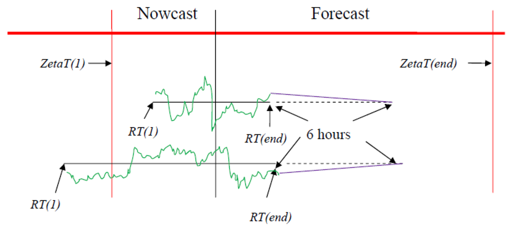
Figure 7.
Diagram on how measured river stage height is used in COMF.
As water temperatures are not available for the two USGS stations, the real-time temperature measurement data are obtained from Port Chicago, a NOAA Gauge Station with NOS_ID of 9415144. When no real-time stage non-tidal data are available from the NCEP data tank, the climatological stage height and temperature data are automatically input into the model.
6.2. Semi-Nowcast/Forecast Results
The SFBOFS semi-operational nowcast and forecast model assessment period started from 10 March 2013 and continued to 10 June 2013. The results from these simulations were concatenated into continuous time series for analysis using the NOS skill assessment software [17]. The model ran robustly in the whole assessment period. Generally, the results of water level, current, temperature and salinity agree well with observations, and CF, NOF, POF, MDNO, MDPO, WOF and other statistical variables pass the criteria in both nowcast and forecast scenarios. Figure 8, as an example, shows the agreement of model results and observation of water level at three major stations. Refer to Peng and Zhang [42] for complete model skill assessment results at all stations for the water level, current, salinity, and water temperature.
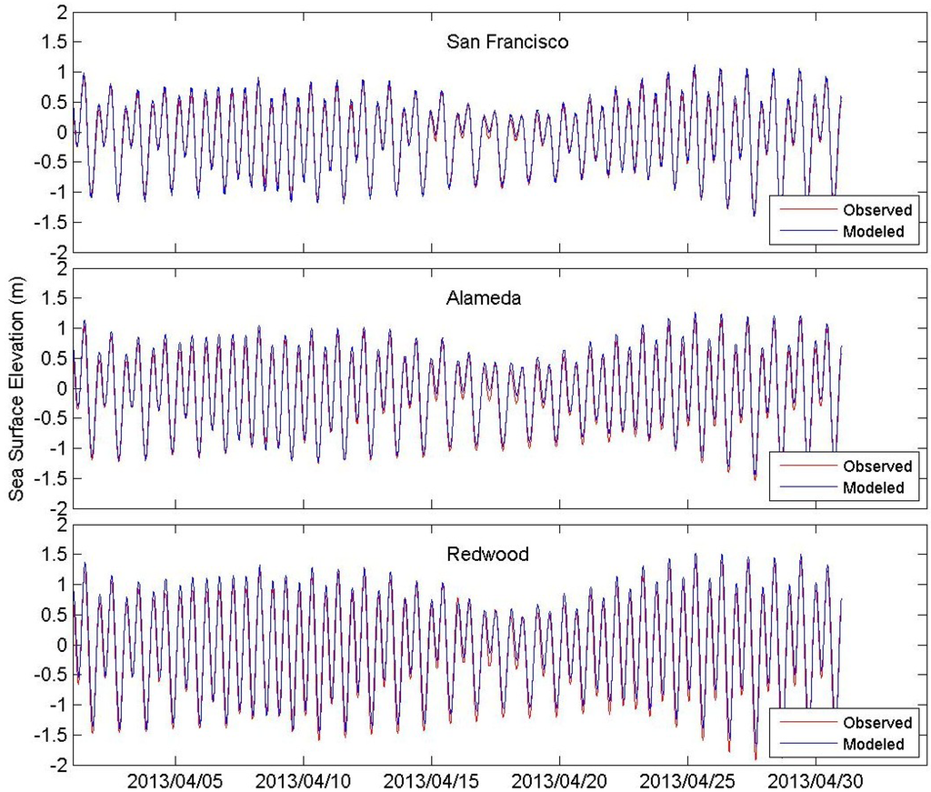
Figure 8.
The comparison of modeled versus observed sea levels at three stations in April 2013. The station locations can be found in Figure 1.
Semi-nowcast/forecast model performance is statistically shown in Figure 9. The Taylor diagrams [43] indicate that the water level results are better than the water temperature and salinity. Water level correlation coefficients at all stations are higher than 0.98, while the salinity correlation coefficient at S1 is only about 0.50 for both nowcast and forecast scenarios. The normalized modeled standard deviation at all stations is close to 1.0 for water level, but it is higher than 2.0 for some stations for salinity. Similar to the hindcast scenarios, as mentioned previously, the water level performs the best followed by water temperature and salinity. One should note that the RMSD value shown in these normalized Taylor diagrams needs to be multiplied by its corresponding measured standard deviation as listed in Table 14, Table 15 and Table 16 to get its real value.
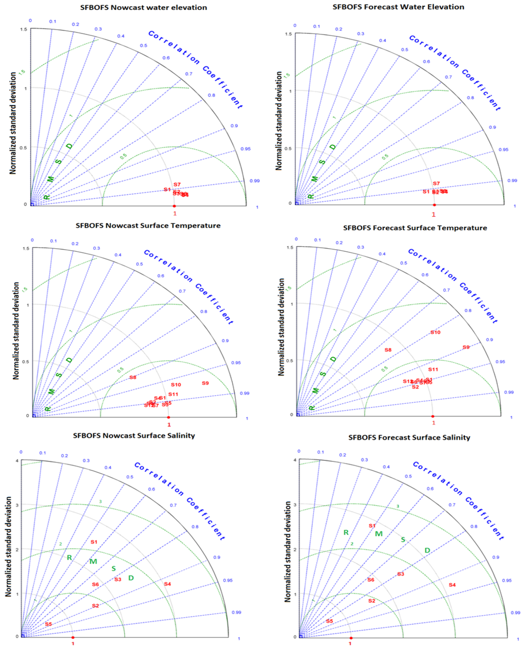
Figure 9.
Normalized Taylor diagrams of water level, surface temperature and surface salinity for nowcast and forecast scenarios. S1, S2, S3, etc. are station series numbers. Si of water level, temperature and salinity does not necessarily indicate the same station. The modeled standard deviation of each variable at each station is normalized by its corresponding observed standard deviation. The data are from October 2013.
Table 14.
Observed water level standard deviations (m) at selected stations in nowcast and forecast scenarios.
| Station # | S1 | S2 | S3 | S4 | S5 | S6 | S7 |
|---|---|---|---|---|---|---|---|
| Station names | Port Chicago | Martinez | Point Reyes | Richmond | San Francisco | Alameda | Redwood City |
| Nowcast | 0.44 | 0.47 | 0.53 | 0.56 | 0.55 | 0.61 | 0.75 |
| Forecast | 0.44 | 0.48 | 0.55 | 0.57 | 0.55 | 0.62 | 0.76 |
Table 15.
Observed temperature standard deviations (°C) at selected stations in nowcast and forecast scenarios.
| Station # | S1 | S2 | S3 | S4 | S5 | S6 |
|---|---|---|---|---|---|---|
| Station Names | Rio Vista | Suisun Slough | Collinsville | Port Chicago | Mallard Island | Martinez |
| Nowcast | 1.52 | 1.87 | 1.48 | 1.48 | 1.42 | 1.43 |
| Forecast | 1.72 | 2.13 | 1.65 | 1.66 | 1.59 | 1.63 |
| Station# | S7 | S8 | S9 | S10 | S11 | S12 |
| Station Names | Antioch | Point Reyes | Richmond | San Francisco | Alameda | Redwood City |
| Nowcast | 1.57 | 0.92 | 0.82 | 0.63 | 1.25 | 1.54 |
| Forecast | 1.66 | 1.06 | 0.95 | 0.73 | 1.46 | 1.83 |
Table 16.
Observed salinity standard deviations (PSU) at selected stations in nowcast and forecast scenarios.
| Station # | S1 | S2 | S3 | S4 | S5 | S6 |
|---|---|---|---|---|---|---|
| Station Names | Suisun Slough | Collinsville | Port Chicago | Mallard Island | Martinez | Antioch |
| Nowcast | 0.40 | 1.10 | 1.56 | 1.35 | 2.18 | 0.95 |
| Forecast | 0.41 | 1.12 | 1.58 | 1.37 | 2.19 | 0.97 |
The semi-nowcast/forecast results can be found on the SFBOFS web page [44]. To serve the San Francisco Bay maritime community, the SFBOFS provides users with nowcast and forecast guidance for water levels, currents, water temperature, and salinity out to 48 h, four times per day. The SFBOFS model domain on the web is divided into two separate subdomains (the San Francisco Bay and the San Francisco Bay Entrance), allowing users to focus on their area of interest. Nowcast/forecast animations of each of the two subdomains as well as time series at over 50 locations are available for winds, water levels, currents, temperature, and salinity.
Figure 10 is a snapshot from nowcast salinity animation of the larger subdomain at 0600 PST of 2 December 2013. Figure 11 illustrates that model salinity results agree well with the measurement at locations where Sacramento and San Joaquin Rivers have noticeable effect on salinity distributions. Meanwhile the available measurement at Port Chicago indicates, as shown in Figure 12, that the water level nowcast is also in good agreement with observations. The satisfying model results for both water level and water salinity near the two rivers are largely due to the fact that river stage boundary conditions have been employed.
The SFBOFS webpage offers not only the latest model output graphics as shown in Figure 10, Figure 11 and Figure 12, but also links where users can get access and download one-year historic output files (in NetCDF format) through CO-OPS’s OPenDAP and THREDDS servers.
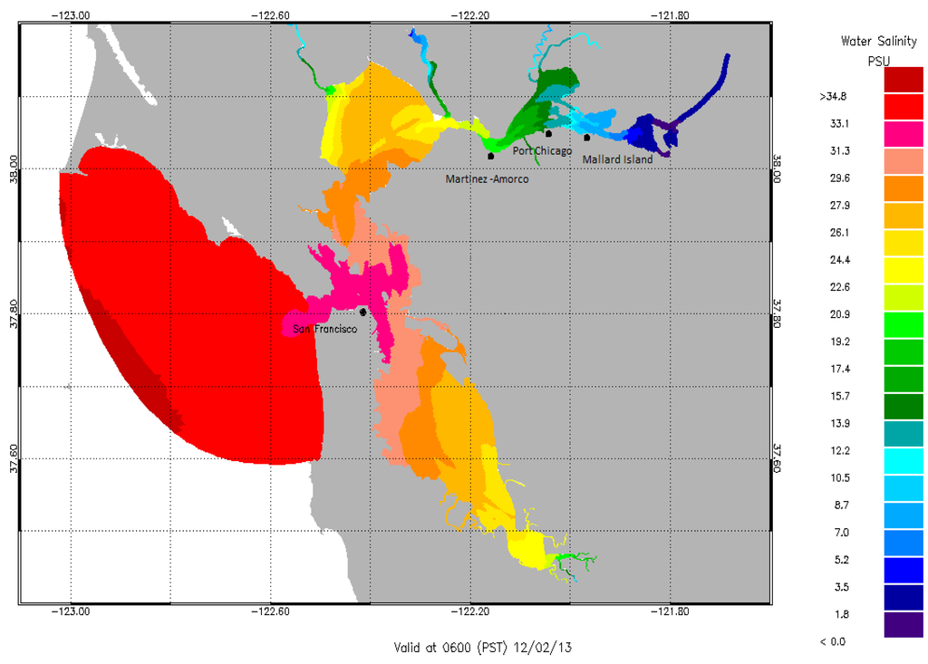
Figure 10.
Nowcast salinity distribution for San Francisco Bay (12/02/13 0600 PST).
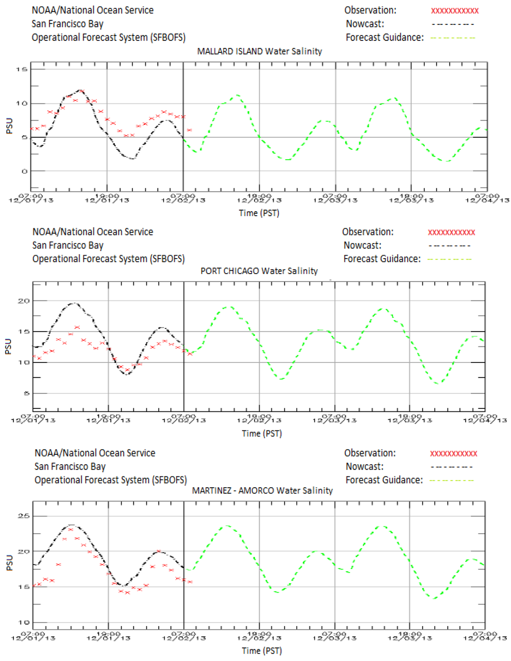
Figure 11.
The nowcast/forecast water surface salinity versus measurement at stations where the Sacramento and San Joaquin Rivers have noticeable effects on salinity distrubution.
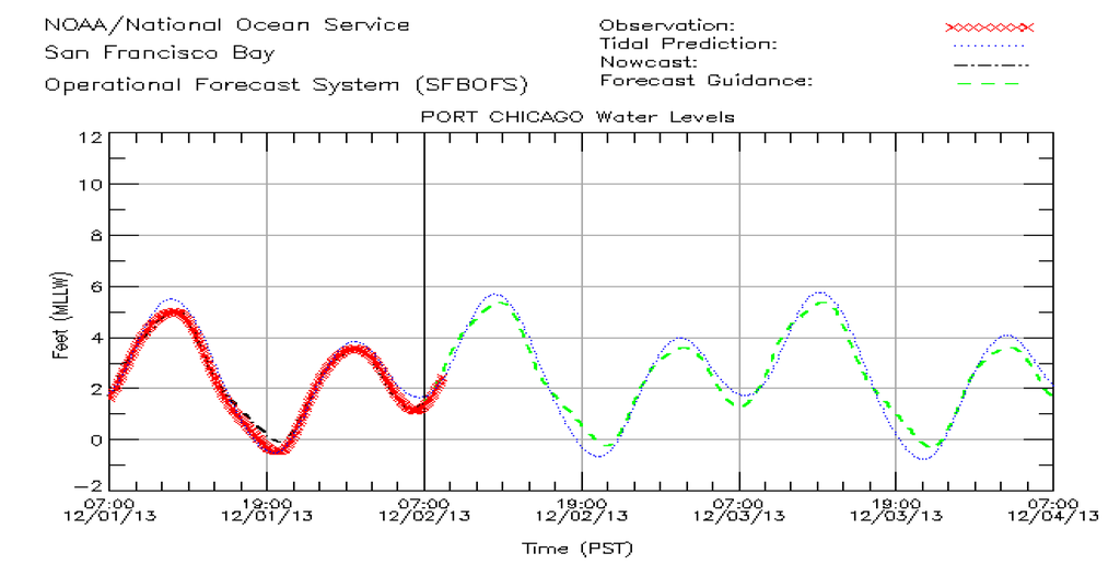
Figure 12.
The nowcast/forecast versus observed water levels at Port Chicago.
7. Conclusion and Discussion
This paper details how the SFBOFS was setup, tested and extensively validated in tidal and hindcast scenarios. The performance of the model package during the three-month semi-operational nowcast and forecast using the NOS COMF-HPC is discussed. FVCOM, the core of SFBOFS, ran robustly during the trial. Amplitudes and epochs of the M2 S2, N2, K2, K1, O1, P1, and Q1 constituents from the tide scenario simulation are very close to the observed values at all stations. NOS skill assessment and RMS errors of all variables indicate that most statistical parameters pass the assessment criteria for both hindcast and nowcast/forecast scenarios and model outputs have good agreements with the measurement. We have to note that OTIS Regional Tide Solutions harmonic analysis results were reduced by 5% on the open boundary. Though this ad hoc treatment ensures very good water level results, more work needs to be done to understand the dynamics behind the adjustment.
Modeled water level and salinity from Martinez to Mallard Island (see Figure 10 for locations) showed strong disagreement with measurement during hindcast period when flow river boundary conditions were employed for the Sacramento and San Joaquin Rivers. The model water level results after using stage river boundary for the two rivers were greatly improved. However, salinity disagreement still existed, though in very low occurrence, during the past ten months after the semi-operational nowcast/forecast trial period. As shown in Figure 13, the model predicted salinity at Port Chicago was in agreement with the observations from October 15–October 25. However, on October 26 and 27, the model salinity predictions at Port Chicago abruptly deviated from the observations. On the 10/27/18Z cycle, the model under predicted the salinity by up to 8 PSU in the nowcast time window. A comparison of the model river forcing water surface elevation to the USGS stage data at the two rivers showed no indication that the model stage was in error.
The location of the river boundaries is still within the tidal domain and either a stage or flow boundary condition is not entirely appropriate. In effect, the boundary location is not at the head of tide and is a tidal river with flow in both directions. In the case of a stage boundary condition, no unique stage discharge relationship exists. The stage is a function of both the discharge and the offshore subtidal water level. The imposition of the stage boundary condition yields accurate water level prediction, but is problematic for salinity, since the appropriate discharge cannot always be specified. For a flow boundary condition, since the boundary is not at the head of tide, tidal wave reflections will occur and will lead to inaccurate stage predictions in the lower delta and even at Port Chicago.
In addition, the model grid cannot represent the complex water channel system in the delta region. One can compare the real delta system in Figure 1 and the model grid in Figure 2. While previous work [15] has used a 20 m deep rectangular “false delta” to produce the appropriate tidal prism of the unresolved area, this approach was not used in the present SFBOFS, since it was felt that the entire delta region may need to be represented as discussed by MacWilliams et al. [45]. This further effort initially considered outside the scope of the SFBOFS is now being considered to improve the salinity prediction in the lower delta and to also potentially provide additional navigation guidance to the Ports of Stockton and Rio Vista. As an interim measure, a data assimilation scheme is being considered within the present SFBOFS, to correct the model salinity predictions from Martinez to Rio Vista on the Sacramento River and Antioch on the San Joaquin River at the start of each nowcast/forecast cycle. Future work will also consider the extension of the offshore boundary to include the Farallon Islands, which will allow for a more accurate specification of the offshore water level and current boundary conditions.
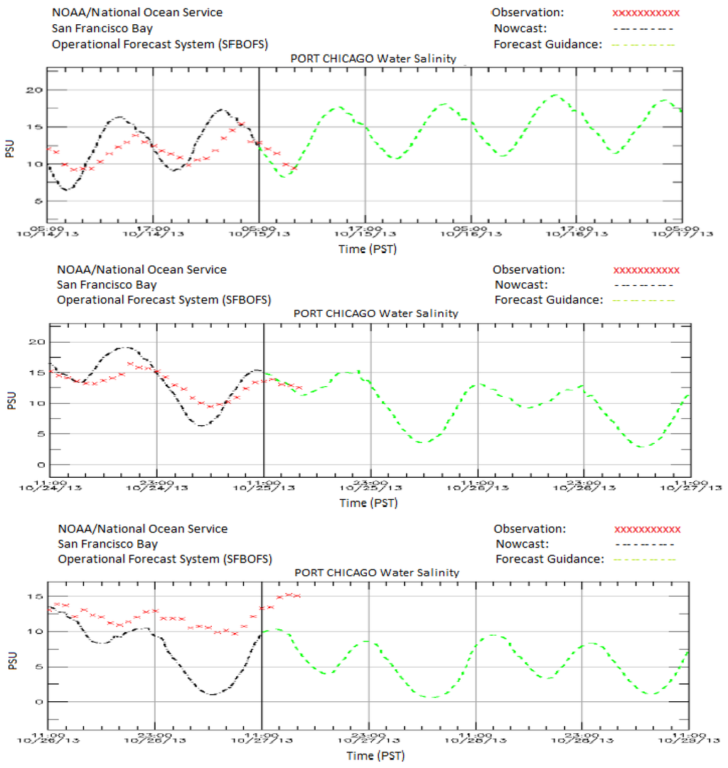
Figure 13.
Modeled salinity strays away from observation with time.
Acknowledgments
Richard Patchen, Chief Science Officer (retired) of the CSDL provided several insights on model grid development. Jiangtao Xu, CSDL, provided valuable assistance with the development of multiple grids and with the use of the SMS software. Philip Richardson, CSDL, assisted with the hindcast initial condition specification, validation data preparation, and the skill assessment. Special thanks to the two anonymous reviewers, who provided many insights and suggestions, which greatly improved the paper.
Author Contributions
R. A. Schmalz and M. Peng conducted hindcast, nowcast and forecast development and are the key authors for the manuscript writing. A. Zhang developed COMF for the operational modeling and supervised the nowcast and forecast development. F. Aikman supervised the hindcast development.
Conflicts of Interest
The authors declare no conflict of interest.
References
- NOAA, National Ocean Service, Center for Operational Oceanographic Products and Services, San Francisco Bay PORTS. Available online: http://tidesandcurrents.noaa.gov/ports/index.html?port=sf (accessed on 15 October 2013).
- Cassuli, V. Semi-Implicit Finite Difference Methods for the Two-Dimensional Shallow Water Equations. J. Comput. Phys. 1990, 86, 56–74. [Google Scholar] [CrossRef]
- Casulli, V.; Cattani, E. Stability, Accuracy and Efficiency of A Semi-Implicit Method for Three-Dimensional Shallow Water Flow. Appl. Math. Comput. 1994, 27, 99–112. [Google Scholar] [CrossRef]
- Casulli, V.; Walters, R.A. An Unstructured Grid, Three-Dimensional Model Based on the Shallow Water Equations. Int. J. Numer. Meth. Fluids 2000, 32, 331–348. [Google Scholar] [CrossRef]
- Cheng, R.T.; Smith, R.E. A Nowcast Model for Tides and Tidal Currents in San Francisco Bay, California. In Proceedings of Ocean Community Conference, Baltimore, MD, USA, 15–19 November 1998; pp. 537–543.
- Gross, E.S.; MacWilliams, M.L.; Kimmerer, W.J. Three-Dimensional Modeling of Tidal Hydrodynamics in the San Francisco Estuary. San Franc. Estuary Watershed Sci. 2010, 7, 1–37. [Google Scholar]
- MacWilliams, M.L.; Cheng, R.T. Three-Dimensional Hydrodynamic Modeling of San Pablo Bay on an Unstructured Grid. In Proceedings of the 7th International Conference on Hydroscience and Engineering, (ICHE-2006); Philadelphia, PA, USA: 10–13 September 2006.
- Barnard, P.L.; Hanes, D.M.; Rubin, D.M.; Kvitek, R.G. Giant Sand Waves at the Mouth of San Francisco Bay. EOS Trans. Am. Geophys. Union 2006, 87, 285–289. [Google Scholar] [CrossRef]
- Barnard, P.L.; Eshleman, J.L.; Erikson, L.H.; Hanes, D.M. Coastal Processes Study at Ocean Beach, San Francisco, CA: Summary of Data Collection 2004–2006; Open File Report 2007-1217; U. S. Geological Survey: Reston, VA, USA, 2007.
- Barnard, P.L.; O’Reilly, B.; van Ormondt, M.; Elias, E.; Ruggiero, P.; Erikson, L.H.; Hapke, C.; Collins, B.D.; Guza, R.T.; Adams, P.N.; et al. The Framework of a Coastal Hazards Model-A Tool for Predicting the Impact of Severe Storms; Open File Report 2009-1073; U. S. Geological Survey: Reston, VA, USA, 2009.
- Deltares. Delft3D-FLOW User Manual; Deltares Rotterdamseweg: Delft, The Netherlands, 2014; p. 684. [Google Scholar]
- Uslu, B.; Arcas, D.; Titov, V.V.; Venturato, A.J. PMEL Tsunami Forecast Series: Vol. 3. A Tsunami Forecast Model for San Francisco, California; NOAA/OAR Special Report, NOAA/PMEL Contribution No. 3342; NOAA/PMEL Center for Tsunami Research: Seattle, WA, USA, 2010.
- Fringer, O.B.; Gerritsen, M.; Street, R.L. An Unstructured-Grid, Finite Volume, Nonhydrostatic, Parallel Coastal Ocean Simulator. Ocean Model. 2006, 14, 139–173. [Google Scholar] [CrossRef]
- Chua, V.P.; Fringer, O.B. Sensitivity Analysis of Three-Dimensional Salinity Simulations in North San Francisco Bay Using the Unstructured-Grid SUNTANS Model. Ocean Model. 2011, 39, 332–350. [Google Scholar] [CrossRef]
- Cheng, R.T.; Casulli, V.; Gartner, J.W. Tidal Residual Intertidal Mudflat (TRIM) Model and its Applications to San Francisco Bay, California. Estuar. Coast. Shelf Sci. 1993, 36, 235–280. [Google Scholar] [CrossRef]
- MacWilliams, M.L.; Gross, E.S.; DeGeorge, J.F.; Rachielle, R.R. Three-Dimensional Hydrodynamic Modeling of the San Francisco Estuary on an Unstructured Grid. In Proceedings of the 32nd International Association for Hydraulic Research Congress, Venice, Italy, 1–6 July 2007.
- Zhang, A.; Yang, Z. Coastal Ocean Modeling Framework on NOAA’s High Performance Computer (COMF-HPC); NOAA Technical Report NOS CO-OPS 039; National Oceanic and Atmospheric Administration: Silver Spring, MD, USA, 2014; p. 70.
- Chen, C.; Liu, H.; Beardsley, R.C. An Unstructured, Finite-Volume, Three-Dimensional, Primitive Equation Ocean Model: Application to Coastal Ocean and Estuaries. J. Atmos. Ocean. Technol. 2003, 20, 159–186. [Google Scholar] [CrossRef]
- Chen, C.; Beardsley, R.C.; Cowles, G.W. An Unstructured Grid, Finite-Volume Coastal Ocean Model (FVCOM) System. Oceanography 2006, 19, 78–89. [Google Scholar] [CrossRef]
- Chen, C.; Beardsley, R.C.; Cowles, G.W. An Unstructured Grid, Finite-Volume Coastal Ocean Model FVCOM User Manual; Technical Report SMAST/UMASSD-06-0602; University of Massachusetts-Dartmouth: New Bedford, MA, USA, 2006. [Google Scholar]
- Xu, J.; Myers, E.P.; White, S.A. VDATUM for the Coastal Waters of North/Central California, Oregon and Western Washington: Tidal Datums and Sea Surface Topography; NOAA Technical Memorandum, NOS CS 22; National Oceanic and Atmospheric Administration: Silver Spring, MD, USA, 2009.
- Schmalz, R.A. Hydrodynamic Model Development for the San Francisco Bay Operational Forecast System (SFBOFS); NOAA Technical Report NOS CS 34; National Oceanic and Atmospheric Administration: Silver Spring, MD, USA, 2014.
- Warner, J. Re: Problem with ROMS Wetting/Drying and Turbulence Model(s); ROMS Discussion Group. Available online: http://www.myroms.org (accessed on 6 February 2012).
- Lettman, K. Personal Communication, University of Oldenburg: Oldenburg, Germany, 2012.
- Fang, X.; Stefan, H.G. Dynamics of Heat Exchange between Sediment and Water in a Lake. Water Resour. Res. 1996, 32, 1719–1727. [Google Scholar] [CrossRef]
- Smith, N. Observations and Simulations of Water-Sediment Heat Exchange in a Shallow Coastal Lagoon. Estuaries 2002, 25, 483–487. [Google Scholar]
- Xue, H.; Due, Y. Implementation of a Wetting-and-Drying Model in Simulating the Kennebec-Androscoggin Plume and the Circulation in Casco Bay. Ocean Dyn. 2010, 60, 341–357. [Google Scholar] [CrossRef]
- Uchiyama, Y. Modeling Three-Dimensional Cohesive Sediment Transport and Associated Morphological Variation in Estuarine Intertidal Mudflats; Port and Airport Research Institute: Yokosuka, Japan, 2005. [Google Scholar]
- Oey, L. A Wetting-Drying Scheme for POM. Ocean Model. 2005, 9, 133–150. [Google Scholar] [CrossRef]
- Oey, L. An OGCM with Movable Land-Sea Boundaries. Ocean Model. 2006, 13, 176–195. [Google Scholar] [CrossRef]
- Oey, L.; Ezer, T.; Hu, C.; Muller-Karger, F.E. Baroclinic Tidal Flow and Inundation Processes in Cook Inlet, Alaska: Numerical Modeling and Satellite Observations. Ocean Dyn. 2007, 57, 205–221. [Google Scholar] [CrossRef]
- California Department of Natural Resources, DAYFLOW program. Available online: http://www.water.ca.gov/dayflow/documentation/dayflowDoc.cfm#Introduction (accessed on 15 October 2010).
- Oltmann, R.N. Indirect Measurement of Delta Outflow using Ultrasonic Velocity Meters and Comparison with Mass-Balance Calculated Outflow; Interagency Ecological Program (IEP) for the Sacramento-San Joaquin Estuary Newsletter: San Francisco, CA, USA, 1998.
- MacWilliams, M. Personal Communication, Delta Modeling Associates: San Francisco, CA, USA, 2013.
- Oregon State University Tidal Data Inversion, OTIS Regional Tide Solutions, 2010: West Coast of the USA. Available online: http://volkov.oce.orst.edu/tides/WC.html (accessed on 15 June 2011).
- Conkright, M.E.; Boyer, T.P.; Antonov, J.I.; Baranova, O.K.; Garcia, H.E.; Gelfeld, R.; Johnson, D.; Locarnini, R.A.; Murphy, P.P.; O’Brien, T.D.; et al. World Ocean Database 2001, Volume 5: Temporal Distribution of Nutrient Profiles; NOAA Atlas NESDIS 46; Levitus, S., Ed.; U.S. Government Printing Office: Washington, DC, USA, 2002; p. 286.
- Carter, G.S. Barotropic and Baroclinic M2 Tides in the Monterey Bay Region. J. Phys. Oceanogr. 2010, 40, 1766–1783. [Google Scholar] [CrossRef]
- Carter, G.S.; Fringer, O.B.; Zaron, E.D. Regional Models of Internal Tides. Oceanography 2012, 25, 56–65. [Google Scholar] [CrossRef]
- Willmott, C.J.; Ackleson, S.G.; Davis, R.E.; Feddema, J.J.; Klink, K.M.; Legates, D.R.; O’Donnell, J.; Rowe, C.M. Statistics for the Evaluation and Comparison of Models. J. Geophys. Res. 1985, 90, 8995–9005. [Google Scholar] [CrossRef]
- Hess, K.W.; Gross, T.F.; Schmalz, R.A.; Kelley, J.G.W.; Aikman, F.; Wei, E.; Vincent, M.S. NOS Standards for Evaluating Operational Nowcast and Forecast Hydrodynamic Model Systems; NOAA Technical Report NOS CS 17; National Oceanic and Atmospheric Administration: Silver Spring, MD, USA, 2003.
- Zhang, A.; Hess, K.W.; Wei, E.; Myers, E. Implementation of Model Skill Assessment Software for Water Level and Current in Tidal Regions; NOAA Technical Report NOS CS 24; National Oceanic and Atmospheric Administration: Silver Spring, MD, USA, 2006.
- Peng, M.; Zhang, A. San Francisco Bay Operational Nowcast and Forecast System Development and its Skill Assessment; NOAA Technical Report (unpublished work); National Oceanic and Atmospheric Administration: Silver Spring, MD, USA, 2013.
- Taylor, K.E. Summarizing Multiple Aspects of Model Performance in a Single Diagram. J. Geophys. Res. 2001, 106, 7183–7192. [Google Scholar] [CrossRef]
- NOAA, National Ocean Service, Center for Operational Oceanographic Products and Services, San Francisco Bay OFS. Available online: http://tidesandcurrents.noaa.gov/ofs/sfbofs/sfbofs.html (accessed on 2 December 2013).
- MacWilliams, M.L.; Salcedo, F.G.; Gross, E.S. San Francisco Bay-Delta UnTRIM Model Calibration Report, POD 3-D Particle Tracking Modeling Study; California Department of Water Resources: Sacramento, CA, USA, 2008.
© 2014 by the authors; licensee MDPI, Basel, Switzerland. This article is an open access article distributed under the terms and conditions of the Creative Commons Attribution license (http://creativecommons.org/licenses/by/3.0/).