Abstract
Understanding the evolution of the sandbar–trough system under regular wave conditions is essential for revealing the dynamic responses of coastal morphology in non-extreme environments and provides a scientific basis for long-term beach stability assessments and coastal erosion management. This study conducted a three-day field observation on Ten-Mile Silver Beach, Hailing Island, China, to investigate the coupling relationships between hydrodynamic factors and bed elevation changes during the morphological evolution of the sandbar–trough system. The results indicate that gravity wave (>0.04 Hz) energy is a key driver of bed elevation changes. During the erosion phase, gravity wave energy increases, and the peak wave energy frequency shifts toward lower frequencies, accompanied by a contraction of low-frequency energy and an expansion of high-frequency energy. In contrast, the accretion phase exhibits the opposite pattern. As the sandbar–trough system developed, the explanatory power of hydrodynamic factors on bed elevation decreased by 41% in the trough region and increased by 3.7% in the sandbar region, indicating a spatially differentiated pattern characterized by weakened forcing in the trough and enhanced response over the sandbar. During the geomorphic adjustment process, the trough area exhibited increased sensitivity, with gravity wave energy, near-infragravity wave (0.01–0.04 Hz) energy, far-infragravity wave (0.004–0.01 Hz) energy, mean wave height, and significant wave steepness reversing their influence directions on bed elevation. In contrast, the sandbar area maintained a more stable hydrodynamic control mechanism, with only the influence pattern of significant wave steepness undergoing a shift. This study enhances the understanding of geomorphology–hydrodynamics coupling within nearshore sandbar–trough systems and provides theoretical insights and technical support for monitoring and evaluating coastal erosion and accretion processes under normal wave conditions.
1. Introduction
Occupying over one-third of the global coastline [1], sandy beaches contribute significantly to socioeconomic development through their recreational, tourism-related, and ecosystem service values [2,3,4]. Sandy beaches play a crucial role in coastal protection by dissipating wave energy, reducing the impacts of storm surges, and serving as natural buffers against coastal hazards [5]. Numerous studies have highlighted the importance of maintaining healthy beach systems to mitigate erosion and safeguard coastal communities [6,7]. Sandbars and troughs are fundamental morphological features within sandy beach systems, playing critical roles in coastal dynamics. Sandbars dissipate incoming wave energy, thereby protecting the shoreline from direct wave attack and modulating sediment transport along the coast [8,9,10]. In contrast, troughs act as dynamic conduits for offshore-directed flows, influencing sediment redistribution and facilitating the evolution of nearshore morphology [11,12,13]. The interplay between sandbars and troughs significantly affects beach stability and resilience to storm events. Climate change and associated sea-level rise are expected to significantly alter the morphodynamic behavior of sandbar–trough systems [14]. Increased storm intensity and elevated mean sea levels can enhance sandbar migration rates, deepen nearshore troughs, and reduce sandbar stability, ultimately leading to accelerated shoreline retreat and disruption of the seasonal morphodynamic cycles [15]. Investigating the hydrodynamic control mechanisms of sandbars and troughs is crucial for predicting beach morphological evolution, sediment transport, and coastal erosion–accretion processes, providing scientific support for coastal ecological protection and management.
A substantial amount of research has been conducted on the long-term evolution of sandbars and troughs. Valsamidis and Reeve [16] developed an analytical model to simulate shoreline evolution near a groyne and a river, highlighting that sandbar formation is primarily governed by the interaction between fluvial sediment supply and longshore sediment transport, with the groyne significantly influencing the sandbar’s location, morphology, and accumulation timescale. The research by Yuhi et al. [17] indicates that the sandbars on the coast exhibit a cyclical net offshore migration pattern, with a lifecycle of approximately 8 years. New sandbars form nearshore every 4 years and gradually migrate offshore. Hu et al. [18] integrated hydrodynamic and sediment transport processes to simulate the formation and long-term evolution of sandbars, revealing that sandbar development is primarily driven by the convergence of sediment transport pathways under the combined influence of river discharge and tidal currents, with tidal range, sediment supply, and estuarine morphology identified as key factors controlling the dynamic evolution of sandbars. Based on prototype-scale experiments, Ruessink et al. [19] demonstrated that the migration direction of sandbars is significantly influenced by the wave breaking fraction, with a transition from onshore to offshore occurring when approximately 20% or more of the waves break over the sandbar crest. Splinter et al. [20], through a study of sandbars using 9 years of observational data, found that an increase in wave height and water level leads to an increase in sandbar volume, which in turn intensifies erosion in the impact zone. The evolution of sandbars and troughs under extreme weather conditions is also a current research focus. Do et al. [21], using satellite imagery, field surveys, and video monitoring data, observed the formation process of nearshore crescent-shaped sandbars under storm wave conditions. They found that the positive feedback between wave–current dynamics and sediment played a key role in the formation of crescent-shaped sandbars. Castelle et al. [22] revealed that storm wave characteristics, particularly wave period and incident angle, play a critical role in controlling beach and dune erosion patterns. In addition, the pre-storm morphology of sandbars was found to be a key factor influencing the extent and variability of storm-induced coastal changes. Almar et al. [23] pointed out that outer sandbars rapidly migrate offshore during storms, and their crescent shape is disrupted, while inner sandbars are primarily influenced by tidal changes, exhibiting uneven variations. Leonardo et al. [24] found that storms lead to the migration and morphological changes in sandbars, with storm surge waves and tidal effects being the main driving factors. Storms typically cause the shape of sandbars to transition from a more stable form to a more dynamic sandbar structure, especially under conditions of large waves and high tides, resulting in rapid and intense changes in sandbar surface and morphology. Current research on sandbar–trough systems mainly focuses on long-term changes and the impacts of extreme weather events, with less attention given to the high-frequency responses of sandbars and troughs under regular wave conditions.
This study aims to investigate the short-term evolution of sandbar–trough systems under regular wave conditions and the high-frequency response of bed elevation to hydrodynamic forcing. Through the analysis of field observation data, it examines the driving relationships between sandbar–trough morphology and hydrodynamic conditions, with the objective of improving predictive models for coastal management [25,26] and informing mitigation strategies under future climate scenarios [27].
2. Materials and Methods
2.1. Study Area
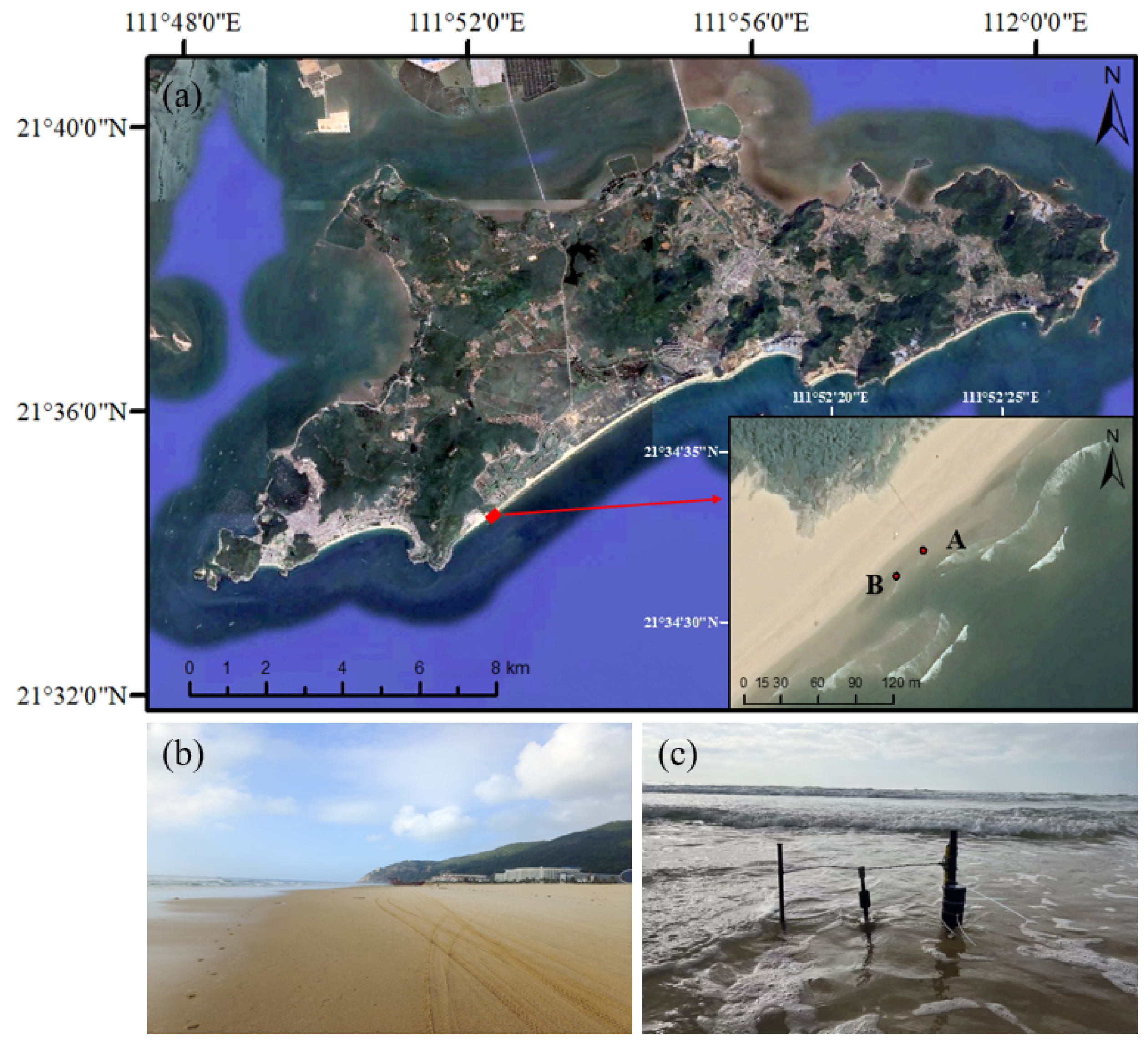
The southern beaches of Hailing Island exhibit a diverse range of geomorphic features, including sandbars and troughs, which are strongly influenced by tidal, wave, and sediment transport processes, resulting in dynamic and evolving nearshore morphology [28]. Hailing Island is located in Yangjiang City, Guangdong Province, China. Ten-Mile Silver Beach, situated on the southern coast of Hailing Island, is an arcuate bay between headlands. The study area is in the southwestern part of Ten-Mile Silver Beach, near a headland, with a width of 80 to 100 m (Figure 1). Based on long-term tidal data from Zhapo Ocean Station (21°35′ N, 111°50′ E) on Hailing Island, the region experiences a mixed semidiurnal tidal regime, with an average tidal range of 1.54 m, a maximum of 3.76 m, and an average spring tidal range of 2.08 m. The local wave climate is characterized by a combination of wind-generated waves and swells, predominantly from the south. Waves exceeding 1.0 m in height occurred 35.8% of the time, with wave periods ranging between 2 and 6 s. The observation period was from 22 to 24 January 2024. During this period, the study area underwent a typical sandbar–trough morphological evolution process, ensuring the adequacy of the data.

Figure 1.
Overview of the study area. (a) Satellite image of the study area; (b) actual photo of the beach; (c) instrument deployment.
The study area exhibits a typical sandbar–trough morphology. Tide and wave recorder and precision autonomous altimeters were deployed at the crest of the sandbar and at the bottom of the trough, respectively (Figure 1c). Although the current study utilizes data from only two locations (points A and B), these points were strategically selected based on their representative positions on the sandbar crest and trough. The spatial-temporal patterns derived from these sites capture the key characteristics of sandbar bed level changes during the observation period. The bed level changes were monitored by two Echologger AA400 (EofE Ultrasonics Co., Ltd., Goyang-si, Republic of Korea) self-recording elevation meters with a sampling frequency of 1 Hz. This is a lightweight, connector-free sonar altimeter that utilizes wireless Bluetooth communication. The instrument calculates the distance from the seabed by emitting a sonar pulse and receiving its echo. The relative bed level change is then computed by subtracting the sonar-measured distance from the known instrument installation height. Wave data were obtained using an RBR Solo3 (RBR Ltd., Ottawa, ON, Canada) tide and wave recorder with a sampling frequency of 2 Hz. The device records underwater pressure fluctuations using a high-precision pressure sensor, which is then used to infer changes in water levels and wave parameters. All instruments were vertically fixed to a steel bracket, with an installation height of 30 cm above the seabed. As these instruments are only reliable when submerged, data collection is interrupted when the instruments are exposed to air during low tide. Due to the effects of wave action, the instruments frequently transition between submerged and exposed states before and after measurements, resulting in irregular data fluctuations. To ensure data quality, measurements collected during these transitional phases were excluded from the analysis.
2.2. Hydrodynamic Data
The water depth data acquired via RBR Solo3 measurements were subjected to spectral analysis to elucidate the distribution pattern of wave energy over various frequency domains. Preprocess the original water depth time series, including detrending to eliminate low-frequency drift, and, if necessary, applying a Hanning window to reduce spectral leakage [29]. Then, employ the Fast Fourier Transform (FFT) to convert the water depth time series from the time domain to the frequency domain [30]. When calculating wave parameters, the pressure spectrum is corrected to the surface elevation spectrum:
In Equation (1), represents the surface elevation spectrum, which describes the wave energy spectral density at the free surface. is the pressure spectrum, obtained from a pressure sensor deployed at a certain depth below the water surface. denotes the wavenumber. is the total water depth, and is the elevation of the pressure sensor above the seabed. Accordingly, represents the vertical distance from the sensor to the free surface. denotes the hyperbolic cosine function, which is used to describe the attenuation of wave-induced pressure with depth during wave propagation.
The adopted correction cutoff frequency is
In Equation (2), represents the depth of the instrument below the water surface, and denotes the cutoff frequency. denotes the acceleration due to gravity.
Wave height, wave period, and wave steepness are critical hydrodynamic factors driving morphological evolution in the surf zone [31]. The calculation of wave height and wave period is performed using the zero-crossing method. The zero-crossing method is a classical time-domain approach commonly used to extract individual wave events from surface elevation time series, enabling the calculation of statistical wave parameters such as mean wave height and average wave period [32]. The average wave height is determined by the peak intervals between the zero-crossing points of the wave signal, while the average period is statistically calculated based on the time intervals between these zero-crossing points. The significant wave steepness is computed using the spectral distance method, which evaluates the steepness of the waves by analyzing the frequency distribution characteristics of the wave spectrum. The formula for calculating the spectral distance is as follows:
In Equation (3), denotes the spectral moment of order , represents the surface elevation spectrum, is the frequency, and is the order of the spectral moment.
The formula for the zeroth-order moment is as follows:
The significant wave steepness is subsequently derived based on the zeroth-order moment, as expressed by the following equation:
In Equation (5), is the mean wave period, obtained using the zero-up-crossing method. denotes the hyperbolic tangent function, is the wavenumber, and is the water depth. is the significant wave height, which is calculated as
The variables appearing in the equation and their explanations are shown in Table 1:

Table 1.
Symbols and Definitions.
2.3. Bed Level Data
Due to tidal exposure causing the instrument to be exposed to air, valid water level data at point A is available during four time periods, totaling 35 h and 40 min. In contrast, data at point B spans three time periods, with a total duration of 41 h. The specific time periods are shown in Table 2. The bed elevation data will be used to calculate relative elevation changes, which will be used to determine the erosion or accretion state of the beach.
Table 2.
Time periods with valid bed elevation data.
3. Results
3.1. Bed Level Elevation Changes
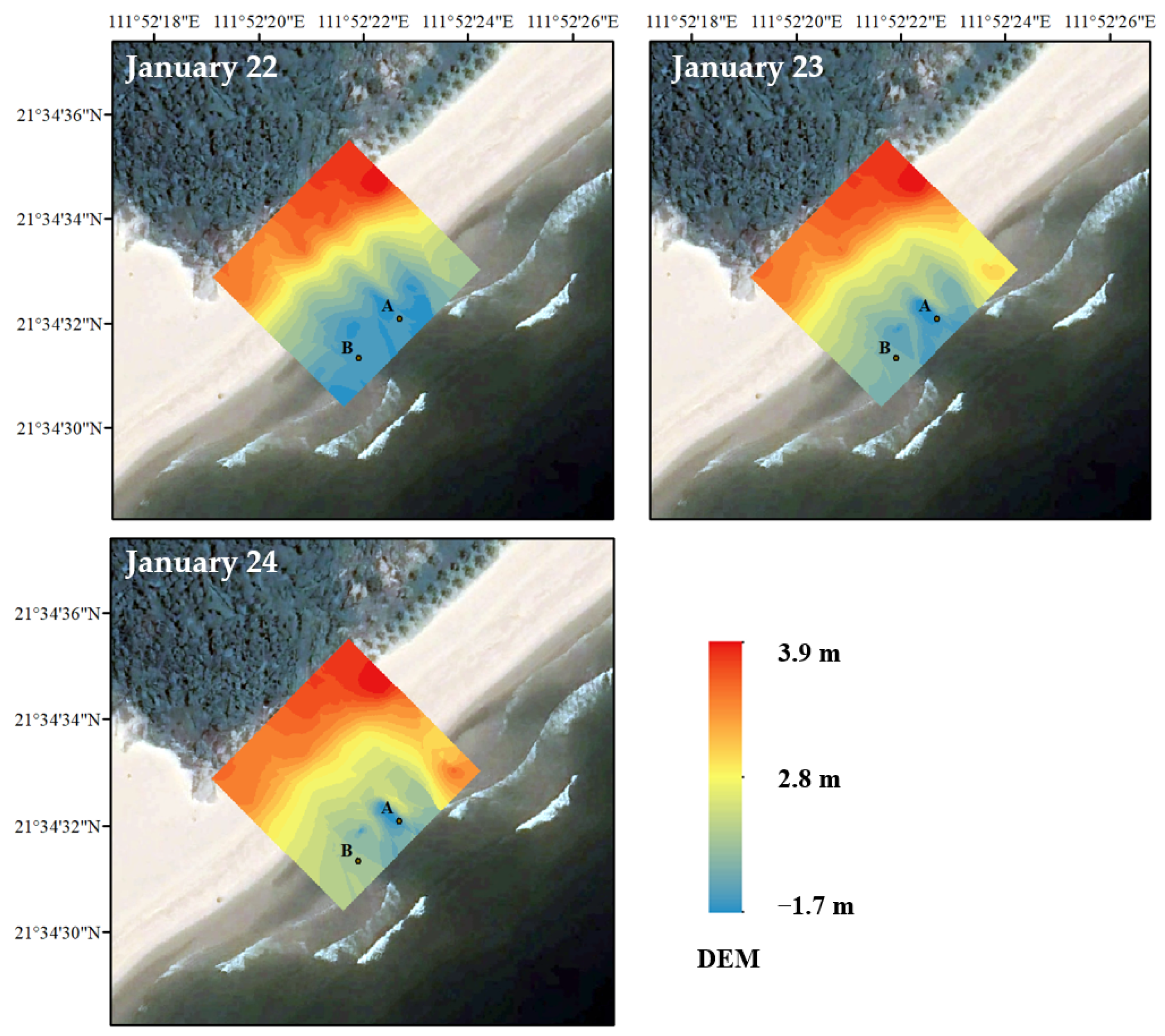
During the observation period, beach elevation was constructed using GPS-RTK and Kriging interpolation [33] (Figure 2). The spherical model was selected as the variogram model. ArcGIS 10.8 automatically fitted the variogram based on the input data and determined the nugget, sill, and range parameters. The root mean square error (RMSE) of the interpolation was 0.143. On the 22nd, the sandbar–trough system had not yet formed. On the 23rd, the elevation at both points A and B decreased, and a significant sandbar–trough system formed. On the 24th, the elevation difference between points A and B continued to increase. The results indicate that during the observation period, the elevation difference between points A and B gradually increased. The dynamic changes in the locations of points A and B during the observation period demonstrate a typical sandbar–trough evolution process.

Figure 2.
Beach elevation model. Beach elevation model constructed by interpolating point elevations measured using GPS-RTK, reflecting the spatial distribution of beach morphology in the study area from 22 to 24 January.
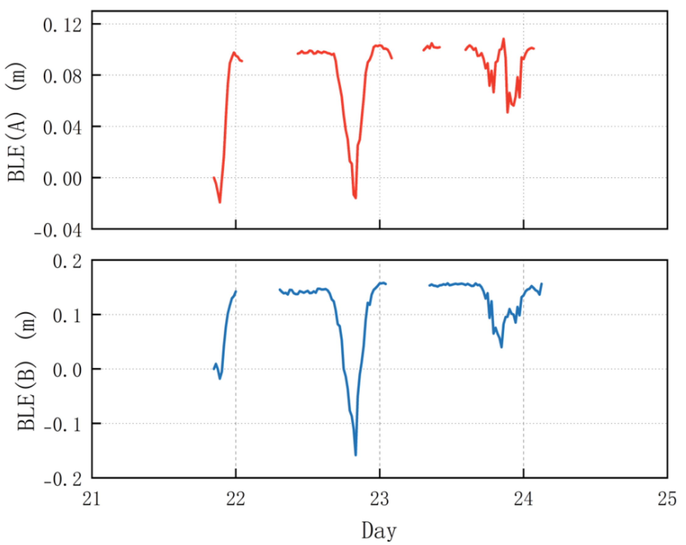
The altimeter recorded the ground clearance at the beginning and end of each pulse, providing the BLE (bed level elevation) change. Figure 3 illustrates the 20 min averaged BLE changes at points A and B. On 22 January, both locations experienced relatively steady erosion and accretion processes. However, on 23 January, BLE fluctuations became significantly more pronounced, particularly at point A, indicating more dynamic morphological changes. The data gaps correspond to periods when the altimeter was exposed above the water surface and stopped recording.
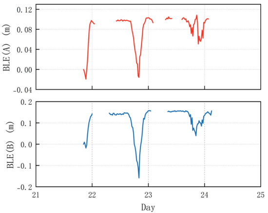
Figure 3.
Twenty-minute time-averaged BLE recorded by PAA. BLE(A) and BLE(B) represent bed level elevation changes at sites A and B, respectively.
On the 22nd, during the erosion phase, point B exhibited a more rapid and intense response, with significant BLE reduction (0.305 m at 0.065 m/h), while point A responded more slowly, initiating erosion about an hour later and showing a smaller BLE decrease of 0.113 m (0.031 m/h). Notably, both points reached their erosion thresholds simultaneously, despite the delayed onset at point A. In the accretion phase, point B again showed a more dynamic response, with a BLE increase of 0.315 m at a rate of 0.079 m/h, whereas accretion at point A was weaker and ceased approximately an hour earlier, with a BLE increase of only 0.118 m (0.039 m/h). These observations suggest that morphological changes at point B were more pronounced throughout the event, likely driven by stronger wave breaking over the sandbar, enhanced wave–current interactions, and higher sediment mobility due to swell influence and wave asymmetry [34,35].
At point A, a distinct sandbar–trough system had formed by the 23rd, as evidenced by the increased elevation difference between points A and B. As shown in Figure 3, point A experienced a complex morphological evolution involving four stages: erosion–accretion–erosion–accretion. The BLE variations at point A occurred approximately one hour earlier than those at point B. The corresponding changes in BLE were 0.036 m, 0.041 m, 0.057 m, and 0.050 m, with rates of 0.009 m/h, 0.025 m/h, 0.085 m/h, and 0.013 m/h, respectively. Notably, the second erosion phase exhibited the greatest amplitude and rate of change.
At point B, the BLE exhibited a similar four-stage pattern, but with less pronounced fluctuations during the second erosion phase. The BLE amplitudes were 0.117 m, 0.070 m, 0.025 m, and 0.067 m, corresponding to change rates of 0.027 m/h, 0.053 m/h, 0.025 m/h, and 0.025 m/h, respectively. Unlike point A, the variation at point B was more moderate during the latter half of the observation period.
These differences suggest that BLE at point A fluctuated more strongly throughout the 23rd, especially during the second erosion phase. This intensified response may be attributed to local hydrodynamic conditions. The presence of the sandbar–trough system likely induced wave focusing within the trough, enhancing local wave height and flow velocity. These concentrated forces could have promoted stronger sediment mobilization and more dynamic morphological adjustments at point A [36,37].
3.2. Hydrodynamic Characteristics
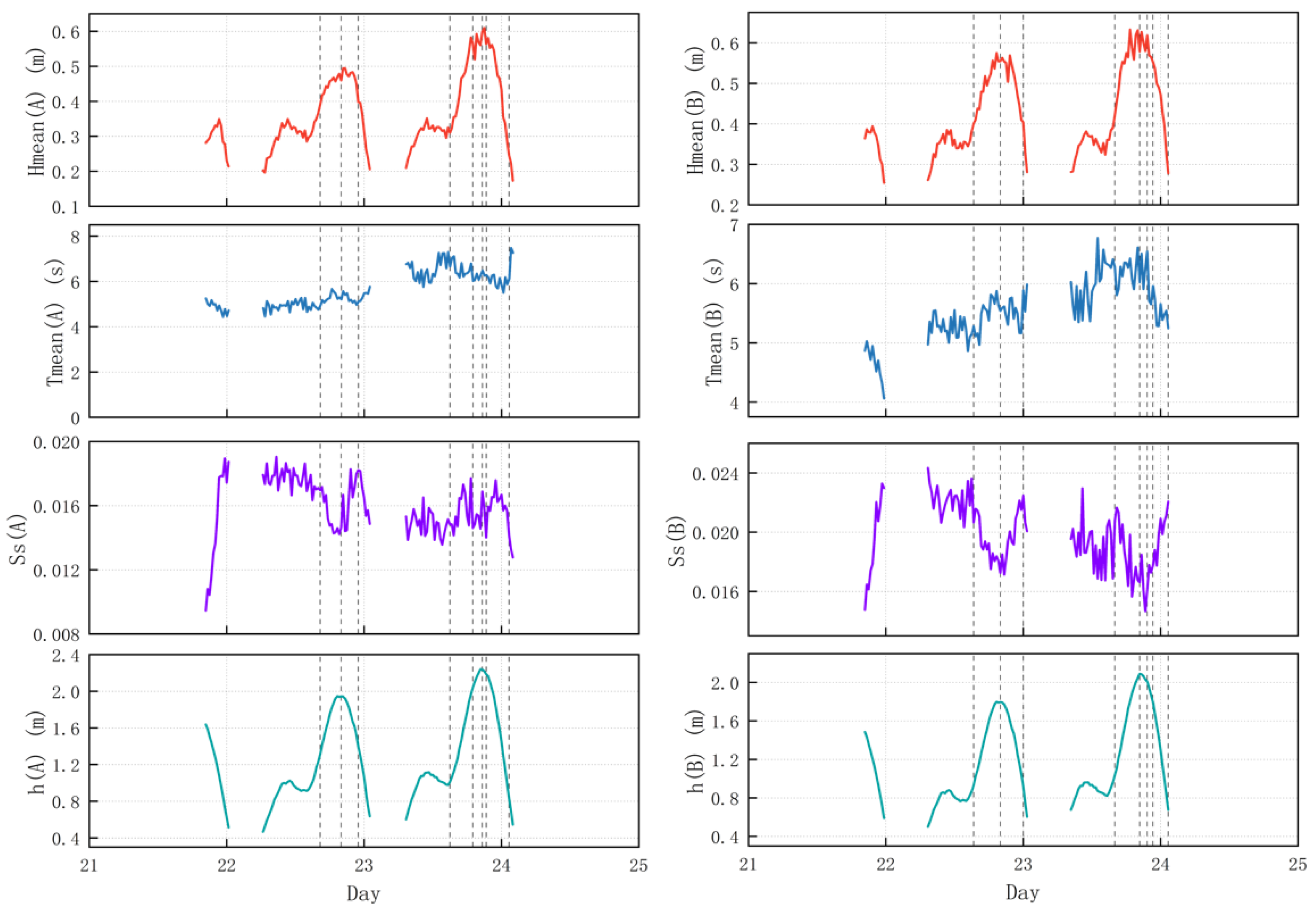
The average wave height (), average wave period (), wave steepness (), and water depth () during the observation period are shown in Figure 4, with the dashed lines indicating erosion and accretion nodes. The identification of erosion and accretion nodes is based on the variation of BLE. Specifically, erosion nodes correspond to a continuous and rapid decrease in BLE, while accretion nodes are characterized by a continuous and rapid increase in BLE.
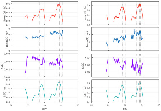
Figure 4.
Wave parameters and water depth (dashed lines indicate bed erosion and accretion nodes).
On the 22nd, during the erosion phase, , , and exhibited an increasing trend, while showed a decreasing trend. The erosion thresholds at point A were 0.391 m (), 4.934 s (), 0.017 (), and 1.314 m (), whereas at point B, the thresholds were 0.401 m (), 5.283 s (), 0.021 (), and 0.93 m (). During the accretion phase, , , and exhibited a decreasing trend, whereas showed an increasing trend. The accretion thresholds at point A were 0.46 m (), 5.21 s (), 0.015 (), and 1.944 m (), while at point B, the thresholds were 0.555 m (), 5.539 s (), 0.017 (), and 1.795 m ().
On the 23rd, BLE exhibited significant fluctuations, and , , and demonstrated pronounced variability throughout the erosion–accretion–erosion–accretion cycle. During the first erosion phase, and at points A and B showed an increasing trend, while and exhibited a decreasing trend. The erosion thresholds at point A were 0.31 m (), 6.664 s (), 0.015 (), and 1.011 m (), whereas at point B, the thresholds were 0.422 m (), 6.282 s (), 0.021 (), and 1.037 m (). During the first accretion phase, at point A, , , , and exhibited an increasing trend, whereas at point B, and showed an increasing trend, while and displayed a decreasing trend. The accretion thresholds at point A were 0.566 m (), 6.02 s (), 0.015 (), and 2.04 m (), while at point B, the thresholds were 0.578 m (), 6.023 s (), 0.017 (), and 2.091 m (). During the second erosion phase, at point A, both wave parameters and water depth exhibited a decreasing trend. At point B, , , and showed a decreasing trend, while exhibited an increasing trend. The erosion thresholds at point A were 0.599 m (), 6.478 s (), 0.017 (), and 2.238 m (), whereas at point B, the thresholds were 0.619 m (), 6.544 s (), 0.016 (), and 2.009 m (). During the second accretion phase, at both points A and B, , , and exhibited a decreasing trend, while showed an increasing trend. The accretion thresholds at point A were 0.564 m (), 6.276 s (), 0.014 (), and 2.187 m (), whereas at point B, the thresholds were 0.552 m (), 5.96 s (), 0.018 (), and 1.793 m ().
On the 22nd, the BLE differences at points A and B were relatively small, and no significant sandbar–trough structure had formed. During the erosion phase, , , and showed an increasing trend, while exhibited a decreasing trend. In the accretion phase, the trends of wave parameters and water depth were opposite to those observed during the erosion phase. The erosion and accretion thresholds for , , and at point B are higher than those at point A, but the water depth threshold is smaller, indicating that the bed at point B requires stronger wave conditions for erosion and accretion to occur, while the bed at point A is more susceptible to changes at greater water depths. On the 23rd, the BLE differences at points A and B increased, with a sandbar forming at point B and a trough forming at point A. During the erosion phase, the threshold for at point B was higher than that at point A, while during the accretion phase, the threshold for at point B was greater than at point A. This indicates that erosion at point B requires higher wave heights to be triggered, and accretion at point B requires steeper waves (with concentrated wave energy and intense breaking) to occur. No similar trends were observed for other parameters, suggesting that the occurrence of erosion and accretion is not solely controlled by a single hydrodynamic factor [38].
4. Discussion
4.1. Spectral Analysis
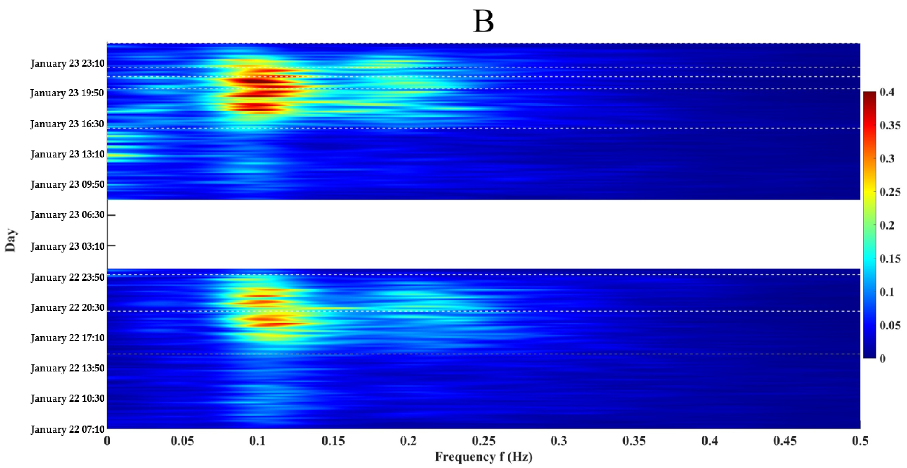
As illustrated in Figure 5 and Figure 6, wave energy is primarily concentrated within the frequency range of 0–0.4 Hz, after which it gradually decreases. The wave energy at point B is generally higher than that at point A.
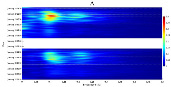
Figure 5.
Frequency spectrum density at point A (white dashed lines indicate erosion and deposition nodes).
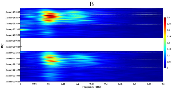
Figure 6.
Frequency spectrum density at point B (white dashed lines indicate erosion and deposition nodes).
On 22 January, during the erosion stage, the wave spectra at both monitoring points exhibited a distinct double-peaked structure. At point A, the two dominant frequency ranges were 0.082–0.139 Hz (low-frequency) and 0.182–0.236 Hz (high-frequency); for point B, the corresponding ranges were 0.074–0.148 Hz and 0.186–0.254 Hz. The peak spectral energy at point A ranged from 0.152 to 0.394 m2 in the low-frequency band and from 0.081 to 0.155 m2 in the high-frequency band. At point B, the corresponding ranges were 0.116–0.508 m2 and 0.059–0.196 m2, respectively. As the degree of erosion increased, the spectral peaks shifted toward lower frequencies, accompanied by a contraction of energy in the low-frequency band and a simultaneous expansion of energy toward higher frequencies. This indicates an enhanced role of high-frequency wave components in sediment mobilization during erosional phases. During the subsequent accretion stage, a similar double-peaked spectral pattern persisted, with peak frequencies and energy magnitudes comparable to those observed during the erosion phase. However, as the accretion progressed, the spectral peaks migrated toward higher frequencies, and the energy in the high-frequency band exhibited a contracting trend. Meanwhile, energy expanded toward the low-frequency band. This reversal in the direction of energy redistribution suggests a contrasting wave–seabed interaction mechanism between erosional and depositional processes.
On 23 January, seabed elevation changes were more pronounced, with considerable spectral fluctuations observed at both points A and B. At point A, the spectral peaks were located within 0.034–0.106 Hz and 0.161–0.273 Hz, with corresponding peak energy values ranging from 0.062 to 0.573 m2 and from 0.025 to 0.203 m2, respectively. At point B, the peak frequency ranges were 0.008–0.109 Hz and 0.160–0.226 Hz, with energy values of 0.096–0.645 m2 and 0.025–0.290 m2, respectively. These results indicate that the first accretion event at point A and the second erosion event at point B corresponded to major fluctuations in bed level. During the first accretion process at point A, spectral peaks shifted toward higher frequencies, high-frequency energy contracted, and energy expanded toward the low-frequency band. Conversely, during the second erosion event at point B, peaks moved toward lower frequencies, low-frequency energy contracted, and energy expanded toward higher frequencies. These patterns were consistent with those observed on 22 January.
Overall, the results demonstrate a close relationship between changes in BLE and the distribution of spectral energy. During erosion, spectral peaks tend to shift toward lower frequencies, with a reduction in low-frequency energy and an expansion toward higher frequencies. In contrast, during accretion, spectral peaks shift toward higher frequencies, accompanied by a contraction of high-frequency energy and an expansion toward the low-frequency band. These results indicate that the frequency position of wave energy peaks and the associated redistribution of spectral energy act as dynamic drivers of BLE change. Specifically, the migration of peak frequencies reflects the dominance of different wave processes that govern sediment transport mechanisms: low-frequency waves are often associated with offshore-directed transport and erosion [39], whereas high-frequency energy tends to promote onshore transport and surface-layer accretion [40]. The observed spectral shifts and energy redistribution patterns therefore imply a physically consistent response of the seabed to changing wave conditions, whereby energy concentration in specific frequency bands alters near-bed shear stress and sediment mobility, ultimately shaping morphological evolution.
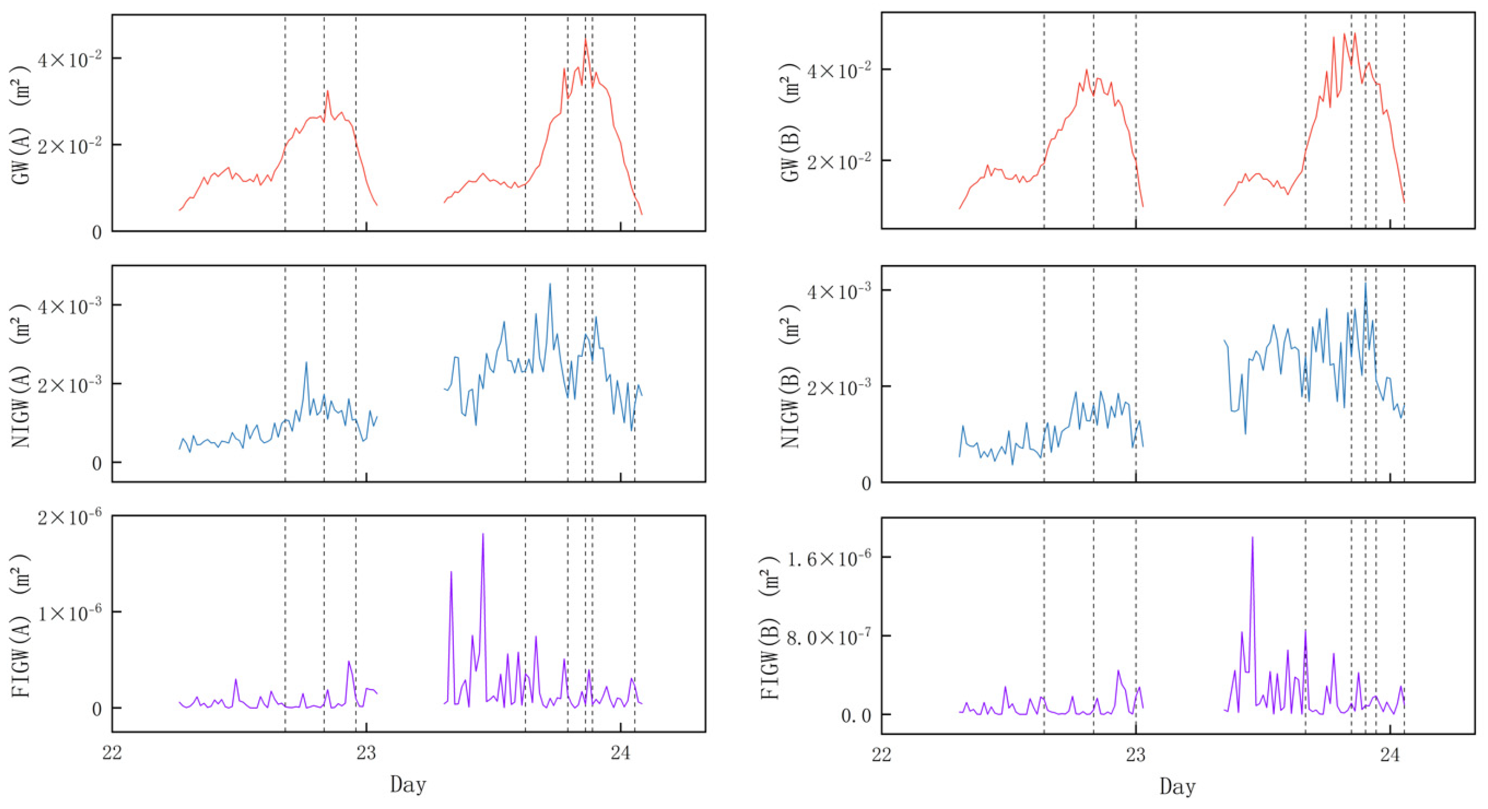
In the study of nearshore dynamics and beach morphology evolution, the influence of wave energy across different frequency bands on coastal processes varies significantly. Gravity waves (GW) (>0.04 Hz), generated by wind, are characterized by short-period fluctuations that typically induce substantial short-term topographical changes due to their strong energy and relatively brief duration of influence [41,42,43]. Near-infragravity waves (NIGW) (0.01–0.04 Hz) possess longer wavelengths and lower frequencies, and their effects on coastal sedimentary processes are more gradual. NIGWs are particularly influential during tidal cycles, seasonal transitions, and storm events, contributing to long-term yet progressive erosion or accretion processes [44,45]. Far-infragravity waves (FIGW) (0.004–0.01 Hz) exhibit even longer wavelengths and lower frequencies, predominantly affecting beach morphology over extended timescales. FIGWs result in widespread and gradual geomorphological changes, exerting a broad and sustained impact [46,47].
The wave energy distribution was determined by integrating the spectral density across the frequency bands, as illustrated in Figure 7. Based on the above results, it can be concluded that changes in BLE are primarily driven by GW energy. By calculating the correlation coefficients between BLE and the energies of GW, NIGW, and FIGW (Table 3), the results indicate that BLE exhibits the strongest correlation with total GW energy. Specifically, GW energy shows a positive correlation with BLE at point A, and a negative correlation at point B. This may be attributed to the enhanced GW energy intensifying wave breaking, leading to increased water turbulence and bottom shear stress, which facilitates the erosion of sediment from the sandbar. The eroded sediment from the sandbar is subsequently transported by the return flow and deposited in the channel region [48]. Furthermore, as the channel deepens and the sandbar builds up, the correlation between GW energy and BLE decreases, particularly in the channel region. This is likely due to geomorphological evolution enhancing the dissipation and regulation of wave energy, thereby reducing the direct forcing effect of wave energy on topographic change. In particular, increased water depth in the channel weakens the bottom disturbance induced by GW, further diminishing the direct coupling between wave energy and morphological response [49].

Figure 7.
Wave energy of GW, NIGW, and FIGW (dashed lines indicate erosion and deposition nodes).
Table 3.
Correlation coefficients between wave energy and BLE.
On 22 January, the BLE remained relatively stable overall. During the erosion phase, GW energy exhibited an increasing trend, followed by a gradual decline during the subsequent accretion phase. On 23 January, BLE changes became more pronounced, showing several short-term local fluctuations. At point A, GW energy generally increased during the erosion phase; however, an 18.42% decrease was observed prior to the first accretion phase, along with a 10.53% decline during the accretion phase. These changes help explain the occurrence of the first accretion event at point A. Before the second erosion phase, GW energy increased significantly, with an amplitude of 32.35%, revealing the potential trigger of the second erosion process at point A. At point B, GW energy generally decreased during the accretion phase on 23 January, but short-term increases of 13.51% were observed during the first accretion and second erosion phases, reflecting the possible driving mechanism behind local BLE fluctuations and the second erosion process at this location. Overall, the spatiotemporal variation of BLE is primarily driven by GW energy, with distinct response mechanisms observed between sandbar and trough regions. Furthermore, as morphological evolution progresses, the driving effect of wave energy on BLE becomes increasingly attenuated.
4.2. Driver Factor Analysis
A multiple linear regression analysis was conducted between BLE and hydrodynamic factors [50], with the results presented in Table 4 and Table 5. The standardized regression coefficient (Beta) was used to evaluate the relative influence of each independent variable on the dependent variable.
Table 4.
Multiple linear regression equation for point A.
Table 5.
Multiple linear regression equation for point B.
On 22 January, the contribution of hydrodynamic factors to BLE at point A was 94.1%, and at point B was 84.8%, indicating that in the absence of a well-developed sandbar–trough structure, hydrodynamic factors exerted a relatively direct influence on BLE variation. By 23 January, as the morphological differentiation between the sandbar and trough became more pronounced, distinct hydrodynamic control mechanisms emerged in different regions. In the trough, increased water depth led to weakened bottom shear and wave-induced disturbance [51], resulting in a reduced explanatory power of hydrodynamic factors for BLE—reflected by a decline in contribution to 45.1%. In contrast, the elevated sandbar became more exposed to wave breaking processes [52], enhancing the sensitivity of BLE to surface disturbances and increasing the contribution of hydrodynamic factors to 88.5%. These findings suggest that morphological evolution can actively modulate the driving capacity of hydrodynamic processes on BLE, leading to spatially differentiated patterns of attenuated forcing or enhanced response at different evolutionary stages.
During the development of the sandbar–trough system, the driving mechanisms of hydrodynamic factors on BLE also underwent significant changes. In the trough region, all hydrodynamic factors except and exhibited shifts in their standardized regression coefficients (Beta values), indicating a reversal or transformation in their influence on BLE. In contrast, during the sandbar elevation process, only showed a change in its driving mechanism. These results suggest that the evolution of the sandbar–trough morphology alters not only the strength but also the direction of the hydrodynamic control on BLE.
In the trough area, multiple hydrodynamic factors exhibited either a reversal in Beta direction or a substantial change in magnitude, reflecting a higher sensitivity of this region to hydrodynamic forcing and stronger feedback from morphological adjustments. Specifically, the Beta value of shifted from –0.592 to 0.052, suggesting that the influence of transitioned from a suppressive effect to a diminished or slightly positive role. This could be attributed to the deepening of the trough, which reduced wave-induced bottom shear and near-bed disturbance due to smoother waveforms. In contrast, Beta values for most hydrodynamic factors at the sandbar location remained relatively stable, implying that this region is more directly affected by continuous wave input. The Beta value of at the sandbar reversed from 0.162 to –0.280, indicating that its influence on BLE shifted from enhancement to suppression, likely due to increased energy dissipation associated with wave breaking over the elevated sandbar.
4.3. Limitations and Implications of the Study
This study, based on field observations, reveals the regulatory role of sandbar–trough morphological evolution in the relationship between wave spectral structure and BLE changes. The results indicate significant differences in spectral peak frequency and spatial distribution of wave energy across different morphological stages. Moreover, morphological changes substantially affect both the strength and direction of hydrodynamic drivers on BLE, exhibiting spatial heterogeneity and dynamic feedback characteristics.
This work enhances the understanding of the coupling mechanisms between morphology and hydrodynamics in nearshore sandbar–trough systems and provides critical support for monitoring and assessing coastal erosion–accretion processes under moderate wave conditions. The findings hold international relevance; similar research has been applied to predict and manage beach morphological changes in high-energy coastal environments such as southeastern Australia [53] and the California coast, USA [54].
Nevertheless, certain limitations remain. First, the observational period primarily captured moderate wave conditions, limiting the ability to assess responses under extreme weather events. Second, while multiple linear regression was employed to identify dominant influencing factors, this method faces significant limitations in representing the nonlinear and strongly coupled dynamics typical of coastal systems, making it inadequate for capturing variable interactions and temporal variability. Future research should expand the temporal and environmental scope of observations and adopt advanced approaches such as machine learning and system identification to enhance explanatory power. Integrating multi-source data with physics-informed models may further advance the understanding of the morphodynamic processes from the perspectives of material transport and energy transformation.
5. Conclusions
This study selected the sandbar–trough system of Ten-Mile Silver Beach on Hailing Island, China, under regular wave conditions, and conducted a three-day field observation to obtain high-frequency and high-precision data on BLE, waves, and other parameters. The evolution of the sandbar–trough system and the variation characteristics of BLE were analyzed, along with the driving factors. The sandbar–trough evolution process exhibits the following characteristics:
- During bed surface erosion, the spectral peak shifts toward lower frequencies, accompanied by a contraction of low-frequency wave energy and an expansion toward higher frequencies. In contrast, during bed accretion, the spectral peak shifts toward higher frequencies, with a reduction in high-frequency energy and a redistribution toward lower frequencies.
- GW energy emerges as the dominant driver of variations in BLE, exhibiting an increasing trend during erosional conditions and a decreasing trend during accretional conditions.
- The process of morphological evolution regulates the influence of hydrodynamic factors on BLE. As the sandbar–trough system developed, the explanatory power of hydrodynamic factors on BLE decreased by 41% in the trough region but increased by 3.7% in the sandbar area, forming a spatially differentiated pattern characterized by attenuated forcing in the trough and enhanced response on the sandbar.
- The evolution of the sandbar–trough morphology altered not only the strength but also the direction of hydrodynamic control on BLE. In the trough region, the influence directions of GW energy, NIGW energy, FIGW energy, , and all exhibited reversals, reflecting a heightened sensitivity of this region to morphological adjustments. In contrast, the sandbar region displayed more stable hydrodynamic driving mechanisms, with only showing a shift in its mode of influence. This indicates that the processes of erosion and accretion are influenced not only by multiple factors but also by topographic feedback.
Author Contributions
Conceptualization, X.B.; methodology, X.B.; writing—original draft preparation, X.B. and Z.L.; review and editing, Y.S., D.Z., T.C., and C.Z. All authors have read and agreed to the published version of the manuscript.
Funding
This research was funded by Guangdong Basic and Applied Basic Research Foundation (No. 2024A1515011427); the National Natural Science Foundation of China (No. 42176167); and Doctoral Research Start-up Fund, Guangdong Ocean University (No. 060302072409).
Data Availability Statement
The data presented in this study are available upon request from the corresponding author.
Conflicts of Interest
The authors declare no conflicts of interest.
References
- Vousdoukas, M.I.; Ranasinghe, R.; Mentaschi, L.; Plomaritis, T.A.; Athanasiou, P.; Luijendijk, A.; Feyen, L. Sandy coastlines under threat of erosion. Nat. Clim. Change 2020, 10, 260–263. [Google Scholar] [CrossRef]
- Luijendijk, A.; Hagenaars, G.; Ranasinghe, R.; Baart, F.; Donchyts, G.; Aarninkhof, S. The state of the world’s beaches. Sci. Rep. 2018, 8, 6641–6651. [Google Scholar] [CrossRef]
- Barbier, E.B.; Hacker, S.D.; Kennedy, C.; Koch, E.W.; Stier, A.C.; Silliman, B.R. The value of estuarine and coastal ecosystem services. Ecol. Monogr. 2011, 81, 169–193. [Google Scholar] [CrossRef]
- Scala, P.; Toimil, A.; Álvarez-Cuesta, M.; Manno, G.; Ciraolo, G. Mapping decadal land cover dynamics in Sicily’s coastal regions. Sci. Rep. 2024, 14, 22222–22237. [Google Scholar] [CrossRef]
- Thiéblemont, R.; Le Cozannet, G.; Rohmer, J.; Toimil, A.; Álvarez-Cuesta, M.; Losada, I.J. Deep uncertainties in shoreline change projections: An extra-probabilistic approach applied to sandy beaches. Nat. Hazards Earth Syst. Sci. 2021, 21, 2257–2276. [Google Scholar] [CrossRef]
- Feagin, R.A.; Sherman, D.J.; Grant, W.E. Coastal erosion, global sea-level rise, and the loss of sand dune plant habitats. Front. Ecol. Environ. 2005, 3, 359–364. [Google Scholar] [CrossRef]
- Narayan, S.; Beck, M.W.; Reguero, B.G.; Losada, I.J.; Van Wesenbeeck, B.; Pontee, N.; Sanchirico, J.N.; Ingram, J.C.; Lange, G.M.; Burks-Copes, K.A. The effectiveness, costs and coastal protection benefits of natural and nature-based defences. PLoS ONE 2016, 11, e0154735. [Google Scholar] [CrossRef]
- Wright Lynn, D.; Short Andrew, D. Morphodynamic variability of surf zones and beaches: A synthesis. Mar. Geol. 1984, 56, 93–118. [Google Scholar] [CrossRef]
- Masselink, G.; Hughes, M.; Knight, J. Introduction to Coastal Processes and Geomorphology; Routledge: Oxfordshire, UK, 2014. [Google Scholar]
- Ferreira, A.M.; Coelho, C.; Silva, P.A. Numerical evaluation of the impact of sandbars on cross-shore sediment transport and shoreline evolution. J. Environ. Manag. 2024, 370, 122835–122849. [Google Scholar] [CrossRef]
- Gallagher, E.L.; Elgar, S.; Guza, R.T. Observations of sand bar evolution on a natural beach. J. Geophys. Res. Ocean. 1998, 103, 3203–3215. [Google Scholar] [CrossRef]
- Saunders, T.M.; Cohn, N.; Hesser, T. Insights into nearshore sandbar dynamics through process-based numerical and logistic regression modeling. Coast. Eng. 2024, 192, 104558–104573. [Google Scholar] [CrossRef]
- Ferreira, A.M.; Coelho, C.; Silva, P.A. Impact of Transversal and Longitudinal Sediment Transport on the Shoreline Evolution: Effects of Sandbar Volume and Wave Climate. J. Coast. Res. 2025, 113, 619–623. [Google Scholar] [CrossRef]
- Chowdhury, P.; Lakku, N.K.G.; Lincoln, S.; Seelam, J.K.; Behera, M.R. Climate change and coastal morphodynamics: Interactions on regional scales. Sci. Total Environ. 2023, 899, 166432–166443. [Google Scholar] [CrossRef] [PubMed]
- Aguilera-Vidal, M.; Muñoz-Perez, J.J.; Contreras, A.; Contreras, F.; Lopez-Garcia, P.; Jigena, B. Increase in the Erosion Rate Due to the Impact of Climate Change on Sea Level Rise: Victoria Beach, a Case Study. J. Mar. Sci. Eng. 2022, 10, 1912–1925. [Google Scholar] [CrossRef]
- Valsamidis, A.; Reeve, D.E. Modelling shoreline evolution in the vicinity of a groyne and a river. Cont. Shelf Res. 2017, 132, 49–57. [Google Scholar] [CrossRef]
- Yuhi, M.; Matsuyama, M.; Hayakawa, K. Sandbar migration and shoreline change on the Chirihama Coast, Japan. J. Mar. Sci. Eng. 2016, 4, 40. [Google Scholar] [CrossRef]
- Hu, P.; Han, J.; Li, W.; Sun, Z.; He, Z. Numerical investigation of a sandbar formation and evolution in a tide-dominated estuary using a hydro-morphodynamic model. Coast. Eng. J. 2018, 60, 466–483. [Google Scholar] [CrossRef]
- Ruessink, B.G.; Blenkinsopp, C.; Brinkkemper, J.A.; Castelle, B.; Dubarbier, B.; Grasso, F.; Puleo, J.A.; Lanckriet, T. Sandbar and beach-face evolution on a prototype coarse sandy barrier. Coast. Eng. 2016, 113, 19–32. [Google Scholar] [CrossRef]
- Splinter, K.D.; Gonzalez, M.V.; Oltman-Shay, J.; Rutten, J.; Holman, R. Observations and modelling of shoreline and multiple sandbar behaviour on a high-energy meso-tidal beach. Cont. Shelf Res. 2018, 159, 33–45. [Google Scholar] [CrossRef]
- Do, J.D.; Jin, J.Y.; Jeong, W.M.; Lee, B.; Kim, C.H.; Chang, Y.S. Observation of nearshore crescentic sandbar formation during storm wave conditions using satellite images and video monitoring data. Mar. Geol. 2021, 442, 106661. [Google Scholar] [CrossRef]
- Castelle, B.; Marieu, V.; Bujan, S.; Splinter, K.D.; Robinet, A.; Sénéchal, N.; Ferreira, S. Impact of the winter 2013–2014 series of severe Western Europe storms on a double-barred sandy coast: Beach and dune erosion and megacusp embayments. Geomorphology 2015, 238, 135–148. [Google Scholar] [CrossRef]
- Almar, R.; Castelle, B.; Ruessink, B.G.; Sénéchal, N.; Bonneton, P.; Marieu, V. Two-and three-dimensional double-sandbar system behaviour under intense wave forcing and a meso–macro tidal range. Cont. Shelf Res. 2010, 30, 781–792. [Google Scholar] [CrossRef]
- Di Leonardo, D.; Ruggiero, P. Regional scale sandbar variability: Observations from the US Pacific Northwest. Cont. Shelf Res. 2015, 95, 74–88. [Google Scholar] [CrossRef]
- Alvarez-Cuesta, M.; Toimil, A.; Losada, I.J. Modelling long-term shoreline evolution in highly anthropized coastal areas. Part 1: Model description and validation. Coast. Eng. 2021, 169, 103960–103984. [Google Scholar] [CrossRef]
- Scala, P.; Manno, G.; Cozar, L.C.; Ciraolo, G. COAST-PROSIM: A Model for Predicting Shoreline Evolution and Assessing the Impacts of Coastal Defence Structures. Water 2025, 17, 269–305. [Google Scholar] [CrossRef]
- Toimil, A.; Losada, I.J.; Nicholls, R.J.; Dalrymple, R.A.; Stive, M.J. Addressing the challenges of climate change risks and adaptation in coastal areas: A review. Coast. Eng. 2020, 156, 103611–103638. [Google Scholar] [CrossRef]
- Hu, P.; Li, Z.; Zhu, D.; Zeng, C.; Liu, R.; Chen, Z.; Su, Q. Field observation and numerical analysis of rip currents at Ten-Mile Beach, Hailing Island, China. Estuar. Coast. Shelf Sci. 2022, 276, 108014–108025. [Google Scholar] [CrossRef]
- Zhiqiang, L.; Zishen, C.; Zhilong, L. Statistical analysis and comparison on wave characteristics during wave propagating in nearshore zone. J. Guangdong Ocean. Univ. 2010, 30, 43–47. (In Chinese) [Google Scholar]
- Monbaliu, J. Spectral wave models in coastal areas. Elsevier Oceanogr. Ser. 2003, 67, 133–158. [Google Scholar] [CrossRef]
- Li, Y.; Zhang, C.; Chen, S.; Qi, H.; Dai, W.; Zhu, H.; Sui, T.; Zheng, J. Experimental investigation on cross-shore profile evolution of reef-fronted beach. Coast. Eng. 2025, 195, 104653–104667. [Google Scholar] [CrossRef]
- Viriyakijja, K.; Chinnarasri, C. Wave flume measurement using image analysis. Aquat. Procedia 2015, 4, 522–531. [Google Scholar] [CrossRef]
- Meng, Q.; Liu, Z.; Borders, B.E. Assessment of regression kriging for spatial interpolation–comparisons of seven GIS interpolation methods. Cartogr. Geogr. Inf. Sci. 2013, 40, 28–39. [Google Scholar] [CrossRef]
- Mieras, R.S.; Puleo, J.A.; Anderson, D.; Hsu, T.J.; Cox, D.T.; Calantoni, J. Relative contributions of bed load and suspended load to sediment transport under skewed-asymmetric waves on a sandbar crest. J. Geophys. Res. Ocean. 2019, 124, 1294–1321. [Google Scholar] [CrossRef]
- van Der Zanden, J.; Hurther, D.; Cáceres, I.; O’Donoghue, T.; Hulscher, S.J.; Ribberink, J.S. Bedload and suspended load contributions to breaker bar morphodynamics. Coast. Eng. 2017, 129, 74–92. [Google Scholar] [CrossRef]
- MacMahan, J.H.; Thornton, E.B.; Reniers, A.J. Rip current review. Coast. Eng. 2006, 53, 191–208. [Google Scholar] [CrossRef]
- Dalrymple, R.A.; MacMahan, J.H.; Reniers, A.J.; Nelko, V. Rip currents. Annu. Rev. Fluid Mech. 2011, 43, 551–581. [Google Scholar] [CrossRef]
- Li, K.; Hao, Y.; Wang, N.; Feng, Y.; Song, D.; Chen, Y.; Zhang, H.; Ren, Z.; Bao, X. Hydrodynamic mechanisms of topographic evolution in straight sandy beach: A case study of Wanpingkou beach, China. Front. Mar. Sci. 2024, 11, 1488610–1488627. [Google Scholar] [CrossRef]
- Su, S.F.; Ma, G.; Hsu, T.W. Numerical modeling of low-frequency waves on a reef island in the South China Sea during typhoon events. Coast. Eng. 2021, 169, 103979–103989. [Google Scholar] [CrossRef]
- Masselink, G.; Austin, M.; Tinker, J.; O'Hare, T.; Russell, P. Cross-shore sediment transport and morphological response on a macrotidal beach with intertidal bar morphology, Truc Vert, France. Mar. Geol. 2008, 251, 141–155. [Google Scholar] [CrossRef]
- Thornton Edward, B.; Guza, R.T. Transformation of wave height distribution. J. Geophys. Res. Ocean. 1983, 88, 5925–5938. [Google Scholar] [CrossRef]
- Masselink, G.; Hughes, M. Field investigation of sediment transport in the swash zone. Cont. Shelf Res. 1998, 18, 1179–1199. [Google Scholar] [CrossRef]
- Scott, T.; Masselink, G.; Russell, P. Morphodynamic characteristics and classification of beaches in England and Wales. Mar. Geol. 2011, 286, 1–20. [Google Scholar] [CrossRef]
- De Bakker, A.T.M.; Tissier, M.F.S.; Ruessink, B.G. Shoreline dissipation of infragravity waves. Cont. Shelf Res. 2014, 72, 73–82. [Google Scholar] [CrossRef]
- Baldock, T.E. Dissipation of incident forced long waves in the surf zone—Implications for the concept of “bound” wave release at short wave breaking. Coast. Eng. 2012, 60, 276–285. [Google Scholar] [CrossRef]
- Masselink, G.; Russell, P. Flow velocities, sediment transport and morphological change in the swash zone of two contrasting beaches. Mar. Geol. 2006, 227, 227–240. [Google Scholar] [CrossRef]
- De Bakker, A.T.M.; Herbers, T.H.C.; Smit, P.B.; Tissier, M.F.S.; Ruessink, B.G. Nonlinear infragravity–wave interactions on a gently sloping laboratory beach. J. Phys. Oceanogr. 2015, 45, 589–605. [Google Scholar] [CrossRef]
- Castelle, B.; Scott, T.; Brander, R.W.; McCarroll, R.J. Rip current types, circulation and hazard. Earth-Sci. Rev. 2016, 163, 1–21. [Google Scholar] [CrossRef]
- Coco, G.; Murray, A.B. Patterns in the sand: From forcing templates to self-organization. Geomorphology 2007, 91, 271–290. [Google Scholar] [CrossRef]
- Uyanık, G.K.; Güler, N. A study on multiple linear regression analysis. Procedia-Soc. Behav. Sci. 2013, 106, 234–240. [Google Scholar] [CrossRef]
- Pascolo, S.; Petti, M.; Bosa, S. On the wave bottom shear stress in shallow depths: The role of wave period and bed roughness. Water 2018, 10, 1348–1366. [Google Scholar] [CrossRef]
- Zhang, W.; Guo, J.; Shi, L.; Liu, Z.; Ye, Q.; Kuang, C.; Peng, Y.; Qi, H. Experimental study on the evolution of submerged artificial sandbar-beach profile under the regular waves condition. Front. Mar. Sci. 2025, 11, 1530904–1530918. [Google Scholar] [CrossRef]
- Short, A.D.; Trembanis, A.C. Decadal scale patterns in beach oscillation and rotation Narrabeen Beach, Australia—Time series, PCA and wavelet analysis. J. Coast. Res. 2004, 20, 523–532. [Google Scholar] [CrossRef]
- Barnard, P.L.; van Ormondt, M.; Erikson, L.H.; Eshleman, J.; Hapke, C.; Ruggiero, P.; Adams, P.N.; Foxgrover, A.C. Development of the Coastal Storm Modeling System (CoSMoS) for predicting the impact of storms on high-energy, active-margin coasts. Nat. Hazards 2014, 74, 1095–1125. [Google Scholar] [CrossRef]

Disclaimer/Publisher’s Note: The statements, opinions and data contained in all publications are solely those of the individual author(s) and contributor(s) and not of MDPI and/or the editor(s). MDPI and/or the editor(s) disclaim responsibility for any injury to people or property resulting from any ideas, methods, instructions or products referred to in the content. |
© 2025 by the authors. Licensee MDPI, Basel, Switzerland. This article is an open access article distributed under the terms and conditions of the Creative Commons Attribution (CC BY) license (https://creativecommons.org/licenses/by/4.0/).