System Identification of a Moored ASV with Recessed Moon Pool via Deterministic and Bayesian Hankel-DMDc

Abstract

This study addresses the system identification of a small autonomous surface vehicle (ASV) under moored conditions using Hankel dynamic mode decomposition with control (HDMDc) and its Bayesian extension (BHDMDc). Experiments were carried out on a Codevintec CK-14e ASV in the CNR-INM towing tank, under both irregular and regular head wave conditions. The ASV under investigation features a recessed moon pool, which induces nonlinear responses due to sloshing, thereby increasing the modeling challenge. Data-driven reduced-order models were built from measurements of vessel motions and mooring loads. The HDMDc framework provided accurate deterministic predictions of vessel dynamics, while the Bayesian formulation enabled uncertainty-aware characterization of the model response by accounting for variability in hyperparameter selection. Validation against experimental data demonstrated that both HDMDc and BHDMDc can predict the vessel’s response under unseen regular and irregular wave excitations. In conclusion, this study shows that HDMDc-based ROMs are a viable data-driven alternative for system identification, demonstrating for the first time their generalization capability for an unseen sea condition different from the training set, achieving high accuracy in reproducing the vessel dynamics.

1. Introduction

The maritime and ocean engineering communities have increasingly recognized the importance of developing accurate and computationally efficient models for the prediction and control of marine system dynamics. In particular, the capability to accurately predict ship motions is essential for supporting design and operations. This holds particularly for seakeeping and maneuvering in adverse weather conditions, for which the availability of reliable predictive tools helps develop and operate vessels, ensuring the safety of structures, payload, and crew. In this regard, commercial and military ships must meet the International Maritime Organization (IMO) Guidelines and NATO Standardization Agreements (STANAG), respectively. Both regulatory frameworks emphasize the need for accurate assessments of vessel motions and loads under a wide range of sea conditions, highlighting the importance of robust modeling and simulation tools to support compliance and operational readiness.

The complexity and nonlinear nature of hydrodynamic phenomena involved pose significant challenges to predicting ship responses in waves. Recent works [1,2] demonstrated the ability of computational fluid dynamics (CFD) methods with unsteady Reynolds-averaged Navier–Stokes (URANS) formulations to assess ship performances in waves and extreme sea conditions. Along with the high fidelity of simulations, however, comes their high computational costs. This is particularly true when simulations aim to achieve statistical convergence of relevant quantities of interest, and complex fluid–structure interactions are investigated. Real-time applications, such as control, fault detection, and digital twinning in general, are also limited by the computational resources required from such models.

In this context, data-driven modeling techniques have emerged as powerful alternatives or complements to traditional first-principles approaches. They promise to reduce the computational cost while keeping the fidelity of their estimates comparable to the original data sources. This requires the methods to be properly trained and/or calibrated, which is generally not trivial [3]. Within this framework, system identification provides a structured approach for constructing predictive models able to incorporate key characteristics of the system from high-fidelity numerical tools and/or experiments. Here, we interpret system identification broadly as the development of reduced-order models (ROMs) capable of predicting system responses, independent of whether their parameters correspond directly to physical quantities.

Equation-based reduced order models (ROMs), such as the Maneuvering Modeling Group (MMG) model [4,5], have been developed as physics-based efficient approaches, characterized by fast evaluation, and demonstrated good agreement with experiments and CFD for the maneuvering of displacement ships [6] and twin-hull configurations [7,8] and have been recently studied also for planing hulls [9]. Physics-based models are typically classifiable as white-box (fully equation-based) or grey-box (physiscs-based with data tuning). This characteristic makes their solution highly interpretable, offering insights on the identified system and the involved physical phenomena Despite the promising results, such models typically exhibit a limited adaptability to unmodeled dynamics (white-box) or require a large amount of data from CFD computations or experimental fluid dynamics (EFD) for their training and definition of forcing terms (grey-box).

Data-driven machine learning techniques gained popularity due to their ability to model complex input–output relations in an automated manner directly from data, not requiring the effort of gaining prior knowledge on the system (equation-free approaches). In particular, recurrent neural networks (RNNs) [10] and long short-term memory networks (LSTMs) [3], along with their bidirectional LSTM (BiLSTM) [11,12] variant, have been demonstrated to be effective for building equation-free data-driven models for ship motions and provide multi-step-ahead forecasting of the ship’s motion in several sailing conditions, including calm water and waves [13]. The strength of machine and deep learning methods lies in their ability to capture relevant hidden and nonlinear input–output relations directly from available data, their compactness, and enabling fast evaluation. However, deep learning models typically require large datasets for training (more complex architectures usually require more expensive training) and to generalize effectively. In addition, while powerful, such models are often considered black-box approaches and pose challenges in terms of the physical interpretability of their results.

Among the available methods, the dynamic mode decomposition (DMD) [14,15,16,17] and its methodological variants have recently gained attention due to their ability to extract dominant dynamic features directly from experimental or numerical data, with small or no assumption on the underlying physics, providing interpretable, low-dimensional representations of nonlinear systems. DMD can be classified somewhere between a black-box and a grey-box approach for reduced-order modeling. With the former, DMD shares the data-driven and equation-free structure like other machine learning techniques, such as RNN, LSTM, and BiLSTM. However, DMD-based methods retain a certain level of interpretability thanks to the linear nature of the model. DMD can be considered a method to build a finite-dimensional approximation of the Koopman operator [18], which, in turn, describes a nonlinear dynamical system as a possibly infinite-dimensional linear system [19]. The reduced-order linear model is obtained by DMD from a small set of snapshots of the dynamical system under analysis. The DMD obtains the model with a direct procedure (linear algebra) that, from a machine learning perspective, constitutes the training phase. Its data-driven nature, the fast non-iterative training, and its data-lean characteristics contributed to the popularity of DMD as a reduced-order modeling technique in several fields, such as fluid dynamics and aeroacoustics [14,20,21,22,23], epidemiology [24], neuroscience [25], finance [26].

DMD was applied for the first time to the forecasting of ship dynamics in [27], in which the proof of concept for short-term forecasting of trajectories, motions, and loads of maneuvering ships in waves was given. In [28], the approach was systematically assessed on the same test cases and first extended to the use of an augmented DMD by augmenting the system state with lagged copies of the original states and their derivatives. This approach enabled the modeling of memory effects in the system, improving accuracy over the tested cases compared to the standard formulation. Ref. [29] systematically explored the use of Hankel-DMD (HDMD) for short-term forecasting of ship motions, highlighting its potential for real-time prediction and control applications and digital twinning. One of the first efforts into the development of a DMD-based, data-driven system identification model for ship motions was conducted in [30], using the dynamic mode decomposition with control (DMDc). This incorporates the control variables (e.g., rudder angle) and forcing inputs (e.g., wave elevation) in the system regression, separating their effect from the free evolution of the system. Furthermore, Hankel-DMD with control (HDMDc) was applied to both ship motion and forces prediction, demonstrating the capability of the method to achieve good accuracy without degradation through the prediction time. The HDMDc was then tested on several ship test cases, introducing methodological advancements to face specific challenges, such as the embedding of nonlinear observables in the state and input vectors to address extremely nonlinear responses of planing hulls in slamming [31], and the use of a Tikhonov-regularized least-square formulation for improving the numerical stability of the DMD regression when using noisy experimental data [32].

Quantifying the uncertainty associated with the prediction of a ROM has become increasingly relevant for data-driven modeling, and a key characteristic for its usage in the context of, e.g., multifidelity analysis and optimization. Few approaches for introducing uncertainty quantification in DMD analysis have been presented in the literature so far. Ref. [33] first introduced a probabilistic model by modeling the measurement noise as Gaussian and treating the dynamic modes and eigenvalues as random variables, whose posterior distributions were inferred through Gibbs sampling. Later, ref. [34] presented the bagging optimized-DMD, where Breiman’s statistical resampling strategy was applied to training data, generating ensembles of DMD models and estimating confidence intervals for the extracted modes and eigenvalues. A similar approach was used in [32] and called a frequentist approach: several training signals were used, producing an ensemble of HDMDc models and estimating confidence intervals for time-resolved predictions of ship motions. Refs. [29,30] considered the uncertainty arising from the selection of HDMD and HDMDc hyperparameters: the length of the training sequence and the number of time-lagged copies of the state were separately considered as probabilistic variables with uniform distributions within a suitable range. Monte Carlo sampling was applied to obtain an ensemble of predictions forming a posterior distribution. This concept, referred to as Bayesian, was further developed in [29,30,31,32], where all relevant hyperparameters are considered as stochastic variables at once.

HDMDc and its stochastic extensions enabled the construction of robust, uncertainty-aware ROMs capable of capturing the essential dynamics of marine systems under realistic operating conditions. In practical marine applications, it is crucial that ROMs remain valid across a variety of sea states, wave spectra, and loading conditions. Testing the transferability of DMD-derived models beyond their training datasets, therefore, represents a key step toward their reliable adoption in real-world scenarios. However, despite the growing body of literature on DMD-based modeling in ship dynamics, most studies to date have focused on fixed or well-controlled experimental conditions, with limited exploration of the generalization capabilities of such models when exposed to unseen environments. In [30,31,32], for example, the test set for the DMD-based ROMs was composed from ship’s dynamic responses to unseen forcing wave signals, which, however, represented different realizations of the same sea state, characterized by an identical spectral distribution of wave energy. Consequently, although the wave sequences used for testing were unseen during training, they were statistically consistent with the training conditions, thus not probing the generalization capability of the models to different sea states.

The present work aims to address this gap by investigating specific capability of HDMDc and BHDMDc system identification to generalize beyond the training conditions. A dedicated experimental campaign was performed at the CNR-INM towing tank facility, collecting data from a Codevintec CK-14e autonomous surface vehicle (ASV) subject to irregular and regular head wave conditions. The ASV features a recessed moon pool, which induces significant nonlinearities in the hydrodynamic response, primarily associated with sloshing and piston-like oscillations of the internal free surface. Specifically, the DMD-based ROMs are learned using data from the irregular waves condition and subsequently applied to predict the vessel response in irregular and regular wave conditions. Statistical and probabilistic analyses were employed to quantify prediction accuracy and uncertainty.

The remainder of this paper is organized as follows. Section 2 describes the experimental setup and data acquisition. Section 3 presents the HDMDc and BHDMDc methodologies adopted in the study. Section 6 discusses the identification results and the validation of the models under different sea conditions. Finally, Section 7 summarizes the main findings and outlines perspectives for future research on data-driven modeling of marine systems.

2. Experimental Setup

2.1. Facility and Model

Experimental tests were carried out at the CNR-INM Emilio Castagneto seakeeping basin in Rome. The facility is 220 m long, 9 m wide, and 3.6 m deep. It is equipped with a single-flap wave generator capable of producing both regular and irregular waves: regular waves with wavelengths ranging from 1 to 10 m and corresponding heights from 0.1 to 0.45 m, as well as irregular waves following any desired sea spectrum at the appropriate scale. The plunger flap, whose rotation axis is located at 1.80 m below the calm water level (mid-depth), is electro-hydraulically driven by three pumps with a total power of 38.5 kW. Its deflection angle is controlled in the range ±13 deg through an electronic programming system producing harmonic components, each modulated in both amplitude and frequency (in the range 0.1–1.4 Hz).

A Codevintec CK-14e ASV was used for the present work, see Figure 1a. The vessel is a small marine surface drone, with a carbon fiber and Kevlar hull, 1.40 m in length ($L_m$), 0.9 m in beam, and 0.35 m in height (0.45 m including the rollbar). In the configuration used for the present tests, the model weighed 60.7 kg, consisting of 22 kg for the hull, 13.4 kg for the batteries, and the remainder for the payload (i.e., instrumentation and cables).

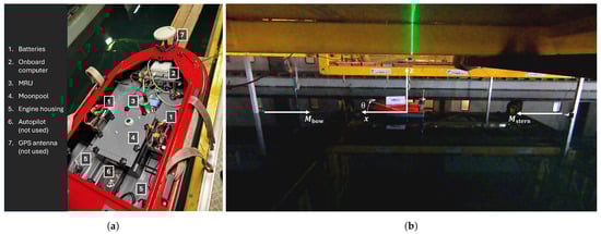
Figure 1. Picture of the CK-14e ASV (a); the top cover is removed, showing the internal configuration and the location of the moon pool, visible from the lid and its fastening system. Towing tank test rig for CK-14e in moored conditions, the white panel used in tracking is visible on the model top cover (b).

2.2. Moored Tests

During the tests, the CK-14e ASV was moored and encountered irregular and regular head waves, as shown in Table 1 and described below.

Table 1. Test matrix; regular and irregular wave conditions.

${\mathit{h}}_{\mathit{s}}$ [m]	${\mathit{\lambda }}_{\mathit{w}}/{\mathit{L}}_{\mathit{m}}$ [-]	${\mathit{v}}_{\mathit{phase}}$ [m/s]	${\mathit{v}}_{\mathit{group}}$ [m/s]	# of Performed Tests
0.15	Pierson-Moskowitz spectrum			3
0.10	1.5	1.811	0.905	1
0.10	2	2.090	1.045	1
0.10	3	2.560	1.280	1

A still carriage in the tank was used to position the bow and stern mooring poles for the model, see Figure 1b; the distance between the two poles was 8.22 m, with the bow pole positioned 48.24 m away from the wave generator flap. The model was moored to the poles through elastic mooring lines, characterized by linear elastic constants $k_{\mathrm{bow}}=1.89$ N/m and $k_{\mathrm{stern}}=1.33$ N/m.

For both regular and irregular wave testing, sea state conditions were selected by considering the CK-14e as a 1:50 scaled model of a 70 m long supply vessel.

2.2.1. Irregular Waves

The first part of the experiments was dedicated to model testing in irregular head waves. The wave generator was operated to produce a linear superposition of $N_w=204$ elemental wave components with random phase $\phi$ and frequencies equally spaced in the interval $0.28$ Hz $\le f\le 1.13$ Hz:

$$\eta \left(t\right)=\sum _{i=1}^{N_w}A\left(f_i\right)sin(2\pi f_{i}t+{\phi }_i).$$

(1)

The amplitudes $A\left(f_i\right)=\sqrt{(4\pi E\left(f_i\right)\Delta f_i)}$ were defined to obtain a sea state 7 Pierson-Moskowitz (P-M) spectrum $E\left(f\right)$ [35] characterized by a significant height of $h_s=0.15$ m and peak period $T_p=2.12$ s in model scale ($h_s=7.5$ m and $T_p=15$ s in full scale):

$$E\left(f\right)={\displaystyle \frac{5}{16}}{h}_s^2{T}_p^{-4}{f}^{-5}exp\left(-{\displaystyle \frac{5}{4}}{T}_p^{-4}{f}^{-4}\right).$$

(2)

Figure 2 compares the nominal power spectral density from Equation (2), with the spectrum obtained from the experimental wave, as measured by the Kenek probe in the forward position (see Figure 3b). The EFD power spectral density is obtained using Welch’s method by analyzing approximately 210 s of wave elevation signal per run (10.5 min) in ASV scale, corresponding to about 4455 s in equivalent supply vessel scale (1 h and 14 min). The signal, sampled at 500 Hz, was divided into segments of $2^{12}$ samples with an overlap of $2^7$ samples. Each segment was transformed using a $2^{16}$-point FFT, and the resulting periodograms were averaged to obtain the final spectral estimate. The actual realizations are characterized by an average significant height of ${\widehat{h}}_s=0.16$ m and average peak period of ${\widehat{T}}_p=1.98$ s in ASV scale (${\widehat{h}}_s=8$ m and ${\widehat{T}}_p=14$ s in equivalent supply vessel scale).

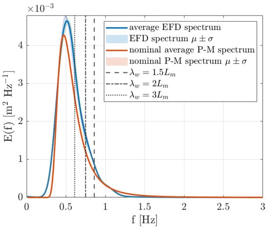
Figure 2. Comparison between nominal Pierson–Moskowitz from Equation (2) and experimental power spectral density of wave elevation obtained from irregular wave test. Vertical lines show the frequencies of regular waves tests.

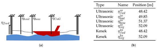
Figure 3. Sketch of the wave probes positions (a), and wave probes location from wave generator flap (b).

2.2.2. Regular Waves

In the second part of the experiments, the moored ASV was subject to regular head waves. The nominal wave height h was set to $h=0.1$ m ASV scale (5 m equivalent supply vessel scale). Three different wavelengths ${\lambda }_w=1.5L_m$, $2L_m$, and $3L_m$ were tested. Actual realizations were characterized by (average ± standard deviation) $\widehat{h}=0.105 \pm 0.01$ m, $0.107 \pm 0.01$ m, and $0.116 \pm 0.01$ m for the three ${\lambda }_w$, respectively.

2.3. Instrumentation

2.3.1. Wave Elevation Measurements

Two capacitance-type probes by Kenek (model SPH 150) were rigidly mounted to the carriage for measuring wave elevation at the forward mooring pole and the center of gravity of the model at rest. In addition, four ultrasonic wave elevation probes were also mounted, two of them in correspondence with the capacitance-type probes, one in correspondence with the half of the forward mooring line at rest, and one in correspondence with the bow of the model at rest. The distance in meters from the wave generator flap to each probe is reported in Figure 3b. The elevation probes collected data with a sampling frequency of $f_{sw}=500$ Hz. Signals were then filtered by applying a low-pass minimum-order filter with delay compensation and stopband attenuation of 60 dB, with passband frequency $f_{pb}=10$ Hz and stopband frequency $f_{sb}=10.75$ Hz.

2.3.2. Motion Measurements

An SMC-108 motion reference unit (MRU) was installed onboard the CK-14e (see Figure 1a), composed of accelerometers and gyroscopes mounted in all three axes. The sensing data signals were acquired with a sampling frequency $f_{sm}=50$ Hz. Measures were processed online in parallel with a Kalman filter inside the MRU multi-core processor. This provided output data for accelerations $\ddot{x},\ddot{y},\ddot{z}$, angular velocities $\dot{\varphi },\dot{\theta }$, heave z, roll $\varphi$, pitch $\theta$, and attitude $\psi$. Furthermore, z was computed by integration of $\ddot{z}$ into a linear position. The integration was further processed and filtered for an accurate heave measurement.

The set of variables was further extended by post processing the measurements: $\dot{x}$ and $\dot{z}$ were obtained by integrating the measured accelerations and $\ddot{\theta }$ were obtained by 4th order central differentiation from the corresponding measured angular velocity. A low-pass minimum-order filter with a stopband attenuation of 60 dB and delay compensation was applied after the integration step, with passband frequency $f_{pb}=10$ Hz and stopband frequency $f_{sb}=10.75$ Hz.

Additionally, a video recording of the moored setup from a side view was taken with a GoPro Hero 7 camera. A dedicated image-processing pipeline was developed to track the motion of the ship model. Each video frame was first converted to the RGB color space and segmented using fixed intensity thresholds to isolate the region corresponding to a white identification panel positioned on top of the model, used as the tracked object. The resulting binary mask was refined through morphological operations (opening, closing, and hole-filling) in order to remove noise and produce a clean and contiguous representation of the target. Connected-component analysis was then performed, and the panel was identified as the largest component. Its geometric properties—including centroid position and orientation angle—were extracted using standard region-based feature analysis. These measurements were stored frame by frame and subsequently low-pass filtered to suppress high-frequency noise and obtain estimations for x, z, and $\theta$. The pitch and heave from the image-processing tracking approach were compared with the MRU signals, obtaining a good agreement, validating the procedure and the so-obtained surge measurement.

2.3.3. Mooring Forces

Mooring forces $M_{\mathrm{bow}}$ and $M_{\mathrm{stern}}$ were measured by two high-accuracy DDEN in-line submersible load cells by Applied Measurements Ltd., Aldermaston, Reading, UK, aligned with the mooring lines at calm water level. Pretensions have been applied accordingly to the elastic constants of the mooring lines and expected motions of the model in the test area.

2.4. Response Amplitude Operators

Figure 4 shows the response amplitude operators (RAOs) for the ASV’s surge, heave, and pitch evaluated from the irregular and regular wave tests data. No significant resonant behavior is evident in the frequency range considered. The RAOs show an overdamped response for the motions; this may be an indication of the moonpool having a dissipative effect through sloshing phenomena, to be confirmed by further investigations which are, however, beyond the scope of this work. Heave and pitch RAOs suggest the presence of a response small peak around ${\lambda }_w/L_{pp}=1.5$, visible in both the irregular and regular response, which is often found in typical seakeeping problems.

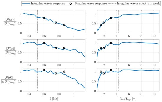
Figure 4. Response amplitude operators for surge, heave, and pitch, evaluated from irregular (solid blue line) and regular (black circles) wave responses. The dash-dotted vertical line highlights the peak frequency of the P-M EFD spectrum.

3. HDMDc

DMD [14,36] was originally presented to decompose high-dimensional time-resolved data into a set of spatiotemporal coherent structures, characterized by fixed spatial structures (modes) and associated temporal dynamics, providing a linear reduced-order representation of possibly nonlinear system dynamics. The original DMD characterizes naturally evolving dynamical systems. In contrast, its extension to forced systems, called DMD with control (DMDc) [37], accounts for the influence of forcing inputs in the analysis, helping disambiguate it from the unforced dynamics of the system.

The standard DMD and DMDc formulations approximate the Koopman operator, creating a best-fit linear model that links sequential data snapshots of measurements [14,15,38]. This model provides a locally linear (in time) representation of the dynamics, which, however, is unable to capture many essential features of nonlinear systems. The augmentation of the system state is thus the subject of several DMD algorithmic variants [17,39,40,41] aiming to find a coordinate system (or embedding) that spans a Koopman-invariant subspace, to search for an approximation of the Koopman operator valid also far from fixed points and periodic orbits in a larger space. However, there is no general rule for defining these observables and guaranteeing they will form a closed subspace under the Koopman operator [42].

The HDMD [43] is a specific version of the DMD algorithm developed to deal with the cases of nonlinear systems in which only partial observations are available [17]. Incorporating time-lagged information in the data used to learn the model, HDMD and HDMDc increase the dimensionality of the system. Including time-delayed data in the analysis, the HDMD and its extension to externally forced systems, HDMDc, can extract linear modes and the associated input operator defined in a space of augmented dimensionality. Such modes are capable of reflecting the nonlinearities in the time evolution of the original system through complex relations between present and past states. The state vector is thus augmented by embedding s time-delayed copies of the original variables. The HDMDc involves, in addition, augmenting the input vector with z time-delayed copies of the original forcing inputs. The use of time-delayed copies as additional observables in the DMD has been connected to the Koopman operator as a universal linearizing basis [44], yielding the true Koopman eigenfunctions and eigenvalues in the limit of infinite-time observations [43].

The HDMDc identifies a representation of the dynamics as an externally forced system:

$${\widehat{\mathbf{x}}}_{j+1}=\widehat{\mathbf{A}}{\widehat{\mathbf{x}}}_j+\widehat{\mathbf{B}}{\widehat{\mathbf{u}}}_j.$$

(3)

The vectors ${\widehat{\mathbf{x}}}_j$ and ${\widehat{\mathbf{u}}}_j$ are referred to as the extended state and input vectors, respectively, at the time instant j. The vectors ${\widehat{\mathbf{x}}}_j$ and ${\widehat{\mathbf{u}}}_j$ are obtained starting from the original state and input vectors ${\mathbf{x}}_j$ and ${\mathbf{u}}_j$, respectively:

$${\mathbf{x}}_j=\left[\begin{array}{c}{x}_1\\ x_2\\ \dots \\ x_N\end{array}\right]\in {\mathbb{R}}^N,{\mathbf{u}}_j=\left[\begin{array}{c}{u}_1\\ u_2\\ \dots \\ u_Q\end{array}\right]\in {\mathbb{R}}^Q,$$

(4)

which are augmented by embedding a number s and z of time-lagged (delayed) copies of the original state and input variables, such that:

$${\widehat{\mathbf{x}}}_j=\left[\begin{array}{c}{\mathbf{x}}_j\\ {\mathbf{x}}_{j-1}\\ \dots \\ {\mathbf{x}}_{j-s}\end{array}\right]\in {\mathbb{R}}^{N(s+1)},{\widehat{\mathbf{u}}}_j=\left[\begin{array}{c}{\mathbf{u}}_j\\ {\mathbf{u}}_{j-1}\\ \dots \\ {\mathbf{u}}_{j-z}\end{array}\right]\in {\mathbb{R}}^{Q(z+1)}.$$

(5)

As a consequence, the extended state matrix and the extended system input matrix are defined as $\widehat{\mathbf{A}}\in {\mathbb{R}}^{N(s+1)\times N(s+1)}$ and $\widehat{\mathbf{B}}\in {\mathbb{R}}^{N(s+1)\times Q(z+1)}$, respectively.

The procedure to extract the extended matrices from data starts by introducing the vector ${\widehat{\mathbf{y}}}_j\in {\mathbb{R}}^{N(s+1)+Q(z+1)}$:

$${\widehat{\mathbf{y}}}_j=\left[\begin{array}{c}{\widehat{\mathbf{x}}}_j\\ {\widehat{\mathbf{u}}}_j\end{array}\right],$$

(6)

such that Equation (3) can be rewritten as follows:

$${\widehat{\mathbf{x}}}_{j+1}=\widehat{\mathbf{G}}{\widehat{\mathbf{y}}}_j,\mathrm{with}\widehat{\mathbf{G}}=\left[\begin{array}{cc}\widehat{\mathbf{A}}& \widehat{\mathbf{B}}\end{array}\right].$$

(7)

Data from m snapshots are re-arranged in two augmented data matrices $\widehat{\mathbf{Y}}\in$${\mathbb{R}}^{\left[N\right(s+1)+Q(z+1\left)\right]\times (m-1)}$ and ${\widehat{\mathbf{X}}}^{\prime }\in {\mathbb{R}}^{N(s+1)\times (m-1)}$, which are built as follows:

$$\widehat{\mathbf{Y}}=\left[\begin{array}{c}\mathbf{X}\\ \mathbf{S}\\ \mathbf{U}\\ \mathbf{Z}\end{array}\right],{\widehat{\mathbf{X}}}^{\prime }=\left[\begin{array}{c}{\mathbf{X}}^{\prime }\\ {\mathbf{S}}^{\prime }\end{array}\right].$$

(8)

Specifically the matrices $\mathbf{X}\in {\mathbb{R}}^{N\times (m-1)}$, ${\mathbf{X}}^{\prime }\in {\mathbb{R}}^{N\times (m-1)}$, and $\mathbf{U}\in {\mathbb{R}}^{Q\times (m-1)}$ contain the state and input snapshots at the m considered time instants:

$$\begin{array}{cc}\hfill \mathbf{X}& =\left[\begin{array}{cccc}{\mathbf{x}}_j& {\mathbf{x}}_{j+1}& \dots & {\mathbf{x}}_{m-1}\end{array}\right],\hfill \end{array}$$

(9)

$$\begin{array}{cc}\hfill {\mathbf{X}}^{\prime }& =\left[\begin{array}{cccc}{\mathbf{x}}_{j+1}& {\mathbf{x}}_{j+2}& \dots & {\mathbf{x}}_m\end{array}\right],\hfill \end{array}$$

(10)

$$\begin{array}{cc}\hfill \mathbf{U}& =\left[\begin{array}{cccc}{\mathbf{u}}_j& {\mathbf{u}}_{j+1}& \dots & {\mathbf{u}}_{m-1}\end{array}\right],\hfill \end{array}$$

(11)

while the Hankel matrices $\mathbf{S}$, ${\mathbf{S}}^{\prime }$, and $\mathbf{Z}$ contain the extended delayed state and input snapshots:

$$\begin{array}{cc}\hfill \mathbf{S}& =\left[\begin{array}{cccc}{\mathbf{x}}_{j-1}& {\mathbf{x}}_j& \dots & {\mathbf{x}}_{m-2}\\ {\mathbf{x}}_{j-2}& {\mathbf{x}}_{j-1}& \dots & {\mathbf{x}}_{m-3}\\ ⋮& ⋮& ⋮& ⋮\\ {\mathbf{x}}_{j-s-1}& {\mathbf{x}}_{j-s}& \dots & {\mathbf{x}}_{m-s-1}\end{array}\right],\hfill \end{array}$$

(12)

$$\begin{array}{cc}\hfill {\mathbf{S}}^{\prime }& =\left[\begin{array}{cccc}{\mathbf{x}}_j& {\mathbf{x}}_{j+1}& \dots & {\mathbf{x}}_{m-1}\\ {\mathbf{x}}_{j-1}& {\mathbf{x}}_j& \dots & {\mathbf{x}}_{m-2}\\ ⋮& ⋮& ⋮& ⋮\\ {\mathbf{x}}_{j-s}& {\mathbf{x}}_{j-s+1}& \dots & {\mathbf{x}}_{m-s}\end{array}\right],\hfill \end{array}$$

(13)

$$\begin{array}{cc}\hfill \mathbf{Z}& =\left[\begin{array}{cccc}{\mathbf{u}}_{j-1}& {\mathbf{u}}_j& \dots & {\mathbf{u}}_{m-2}\\ {\mathbf{u}}_{j-2}& {\mathbf{u}}_{j-1}& \dots & {\mathbf{u}}_{m-3}\\ ⋮& ⋮& ⋮& ⋮\\ {\mathbf{u}}_{j-z-1}& {\mathbf{u}}_{j-z}& \dots & {\mathbf{u}}_{m-z-1}\end{array}\right].\hfill \end{array}$$

(14)

The augmented matrix $\widehat{\mathbf{G}}=\left[\widehat{\mathbf{A}}\widehat{\mathbf{B}}\right]\in {\mathbb{R}}^{N(s+1)\times \left(N\right(s+1)+Q(z+1\left)\right)}$ is approximated by solving the following regularized least-square minimization:

$$\underset{\widehat{A},\widehat{B}}{min}\left|\right|{\widehat{\mathbf{X}}}^{\prime }-\left[\widehat{\mathbf{A}}\widehat{\mathbf{B}}\right]\widehat{\mathbf{Y}}{\left|\right|}_F^2+\lambda \left[\widehat{\mathbf{A}}\widehat{\mathbf{B}}\right]{\left|\right|}_F^2,$$

(15)

which solution is given by the following equation:

$$\left[\widehat{\mathbf{A}}\widehat{\mathbf{B}}\right]={\widehat{\mathbf{X}}}^{\prime }{\widehat{\mathbf{Y}}}^{\mathrm{T}}{\left[\widehat{\mathbf{Y}}{\widehat{\mathbf{Y}}}^{\mathrm{T}}+\lambda \mathbf{I}\right]}^{-1}.$$

(16)

where $\lambda$ is a regularization factor. The above Tikhonov-regularized formulation extends the one presented in [45] to the HDMDc. It is suitable for improving the numerical stability of DMD regression, with its robustness in high-dimensional spaces and accuracy for applications involving noisy data. A similar effect can be pursued with the exact-DMD formulation by SVD rank truncation, see [31], also reducing the model size. The Tikhonov-regularized formulation is here preferred for its more robust behavior to noisy data. Once the matrices $\widehat{\mathbf{A}}$ and $\widehat{\mathbf{B}}$ are obtained, Equation (3) can be used to calculate the time evolution of the augmented state vector $\widetilde{\widehat{\mathbf{x}}}\left(t\right)$ from an initial condition, where the tilde indicates the HDMDc estimation. By isolating its first N components, the predicted time evolution of the original state variables $\tilde{\mathbf{x}}\left(t\right)$ is extracted.

Uncertainty Quantification in HDMDc Through Ensembling

DMD-based models can be further extended to provide uncertainty estimation of their predictions. To this aim, the ensembling approach is applied, i.e., the combination of predictions coming from different models to obtain a prediction along with its statistics. The Bayesian formulation for HDMDc, which leads to BHDMDc was intrduced in [30]. The driving rationale behind the BHDMDc is the observation highlighted by the authors in previous works [13,28] that the final prediction from DMD-based models can strongly vary for different hyperparameter settings. Furthermore, there is no general rule for determining their optimal values.

The dimensions and the values within matrices $\widehat{\mathbf{A}}$ and $\widehat{\mathbf{B}}$ depend on the four hyperparameters m, s, z, and $\lambda$. In place of the the first three, we equivalently use their respective time lengths, i.e., the observation time length $l_{tr}=t_m-t_1$, the maximum delay time in the augmented state $l_{d_x}=t_{j-1}-t_{j-s-1}$, and the maximum delay time in the augmented input $l_{d_u}=t_{j-1}-t_{j-z-1}$. The relation between m, s, z, and $l_{tr}$, $l_{d_x}$, $l_{d_u}$ is given by:

$$m=⌊{\displaystyle \frac{l_{tr}}{\Delta t}}⌋,s=⌊{\displaystyle \frac{l_{d_x}}{\Delta t}}⌋,z=⌊{\displaystyle \frac{l_{d_u}}{\Delta t}}⌋,$$

(17)

with $\Delta t$ the step of the temporal discretization. These dependencies can be denoted as follows:

$$\begin{array}{cc}\hfill \widehat{\mathbf{A}}& =\widehat{\mathbf{A}}(l_{tr},l_{d_x},l_{d_u},\lambda ),\hfill \\ \hfill \widehat{\mathbf{B}}& =\widehat{\mathbf{B}}(l_{tr},l_{d_x},l_{d_u},\lambda ).\hfill \end{array}$$

(18)

In BHDMDc, the hyperparameters are considered as stochastic variables with given prior distribution, $p\left(l_{tr}\right)$, $p\left(l_{d_x}\right)$, $p\left(l_{d_u}\right)$, and $p\left(\lambda \right)$, respectively. Through uncertainty propagation, the solution $\tilde{\mathbf{x}}\left(t\right)$ also depends on $l_{tr}$, $l_{d_x}$, $l_{d_u}$, and $\lambda$:

$$\mathbf{x}=\mathbf{x}(t,l_{tr},l_{d_x},l_{d_u},\lambda ),$$

(19)

and the following are used to define, at a given time t, the expected value ($\mu$) of the solution and its standard deviation ($\sigma$):

$$\mu \left[\mathbf{x}\left(t\right)\right]={\int }_{{\lambda }^l}^{{\lambda }^u}{\int }_{l_{d_u}^l}^{l_{d_u}^u}{\int }_{l_{d_x}^l}^{l_{d_x}^u}{\int }_{l_{tr}^l}^{l_{tr}^u}\mathbf{x}(t,l_{tr},l_{d_x},l_{d_u},\lambda )p\left(l_{tr}\right)p\left(l_{d_x}\right)p\left(l_{d_u}\right)p\left(\lambda \right)d{l}_{tr}d{l}_{d_x}d{l}_{d_u}d\lambda ,$$

(20)

$$\sigma \left[\mathbf{x}\left(t\right)\right]={\left\{{\int }_{{\lambda }^l}^{{\lambda }^u}{\int }_{l_{d_u}^l}^{l_{d_u}^u}{\int }_{l_{d_x}^l}^{l_{d_x}^u}{\int }_{l_{tr}^l}^{l_{tr}^u}{\left\{\mathbf{x}\left(t,l_{tr},l_{d_x},l_{d_u},\lambda \right)-\mu \left[\mathbf{x}\left(t\right)\right]\right\}}^{2}p\left(l_{tr}\right)p\left(l_{d_x}\right)p\left(l_{d_u}\right)p\left(\lambda \right)d{l}_{tr}d{l}_{d_x}d{l}_{d_u}d\lambda \right\}}^{{\displaystyle \frac{1}{2}}},$$

(21)

where $l_{tr}^l$, $l_{d_x}^l$, $l_{d_u}^l,{\lambda }^l$, and $l_{tr}^u$, $l_{d_x}^u$, $l_{d_u}^u$, ${\lambda }^u$ are lower and upper bounds and $p\left(l_{tr}\right)$, $p\left(l_{d_x}\right)$, and $p\left(l_{d_u}\right)$$p\left(\lambda \right)$ are the given probability density functions for $l_{tr}$, $l_{d_x}$, $l_{d_u}$, and $\lambda$.

In practice, a uniform probability density function is assigned to the hyperparameters, and a set of realizations is obtained through a Monte Carlo sampling, obtaining a posterior distribution on the prediction.

We note that the proposed method is termed “Bayesian” in a broader sense than classical Bayesian inference. In particular, posterior distributions are not inferred over the Koopman operator or dynamic mode decomposition matrices themselves. Instead, in BHDMDc, the hyperparameters of the method are treated in a Bayesian manner, assigning them given prior distributions and propagating their uncertainty through Monte Carlo sampling. This results in a predictive distribution for the system variables. While this does not constitute full Bayesian parameter inference, it is consistent with Bayesian principles of uncertainty propagation and model averaging and aligns with how “Bayesian” is used in the related literature for uncertainty-aware reduced-order modeling.

4. Statistical Variables and Performance Metrics

To compare the predictions made by the deterministic and Bayesian models with the ground truth from the experiments, four error indices are employed: the average normalized mean square error (ANRMSE) [13], its time-resolved version ($\epsilon$), the normalized average minimum/maximum absolute error (NAMMAE) [13], and the Jensen-Shannon divergence (JSD) [46].

The ANRMSE quantifies the root mean square error between the predicted values ${\tilde{\mathbf{x}}}_t$ and the measured (reference) values ${\mathbf{x}}_t$ at different time steps, normalizing the result for each variable by k times the standard deviation of the measured value ($k=1$ in this work) and averaging over the N variables in $\mathbf{x}$:

$$\mathrm{ANRMSE}={\displaystyle \frac{1}{N}}\sum _{i=1}^N\sqrt{{\displaystyle \frac{1}{\mathcal{T}{\left(kSD\left[x_i\right]\right)}^2}}{\displaystyle \sum _{j=1}^{\mathcal{T}}}{\left({\tilde{x}}_i\left(t_j\right)-x_i\left(t_j\right)\right)}^2},$$

(22)

where $\mathcal{T}$ is the number of time instants in the considered time window, and $SD\left[\xi \right]$ indicates the standard deviation of the measured values in the considered time window for the variable $\xi$:

$$SD\left[\xi \right]=\sqrt{{\displaystyle \frac{1}{\mathcal{T}-1}}\sum _{i=1}^{\mathcal{T}}{({\xi }_i-EV\left[\xi \right])}^2}$$

(23)

and

$$EV\left[\xi \right]={\displaystyle \frac{1}{\mathcal{T}}}\sum _{i=1}^{\mathcal{T}}{\xi }_i$$

(24)

For the same time window, the time-resolved variant of the ANRMSE called $\epsilon$ is evaluated as the average across the N variables of the time evolution of the square root difference between the reference and predicted signal, normalized by its standard deviation in the considered time interval:

$$\epsilon \left(t\right)={\displaystyle \frac{1}{N}}\sum _{i=1}^N\sqrt{{\displaystyle \frac{{\left(\widetilde{x_i}\left(t\right)-x_i\left(t\right)\right)}^2}{{\left(kSD\left[x_i\right]\right)}^2}}}$$

(25)

This is used to monitor potential trends in the prediction error, i.e., whether the accuracy decreases or increases for longer predictions.

The NAMMAE metric [13] provides an engineering-oriented assessment of prediction accuracy. It measures the absolute difference between the minimum and maximum values of the predicted and measured time series, normalized by k times the standard deviation of the measured values, and averaged over N variables, as follows:

$$\mathrm{NAMMAE}={\displaystyle \frac{1}{2N}}\sum _{i=1}^N{\displaystyle \frac{1}{kSD\left[x_i\right]}}(\left|min\left({\tilde{x}}_i\left(t_j\right)\right)-min\left(x_i\left(t_j\right)\right)\right|+\left|max\left({\tilde{x}}_i\left(t_j\right)\right)-max\left(x_i\left(t_j\right)\right)\right|)j=1,\dots ,\mathcal{T}.$$

(26)

In addition to the direct comparison of DMD-predicted and experimentally measured time histories, calculating the probability density function (PDF) of the variables under prediction is of interest for the application in irregular waves. To statistically assess the PDF estimator obtaining confidence intervals, a moving block bootstrap (MBB) method is applied to time histories from EFD and BHDMDc-based predictions of each variable. For the MBB analysis of a generic variable $\xi$, a single time series of $\mathcal{T}$ items is obtained for the EFD and the BHDMDc, respectively, by joining all the measured or predicted series. From the single time series, a number $C=\mathcal{T}-r+1$ of moving blocks is used, each defining a time series composed by ${\xi }_i$$i=c,\dots ,c+r-1$, where c is the block index, and $r={(2\phi /a)}^{2/3}{\mathcal{T}}^{1/3}$ is an optimal block length [47] with

$$\phi ={\displaystyle \frac{{\displaystyle \mathcal{T}\sum _{i=1}^{\mathcal{T}}\left[{\xi }_{i+1}-\mathrm{EV}\left(\xi \right)\right]\left[{\xi }_i-\mathrm{EV}\left(\xi \right)\right]}}{{\displaystyle (\mathcal{T}-1)\sum _{i=1}^{\mathcal{T}}\left[\left({\xi }_i-\mathrm{EV}\left(\xi \right)\right)\right]}}}$$

(27)

and $a=(1-\phi )(1+\phi )$. From the original set of C blocks, a number of $C^{\prime }=\mathcal{T}/r$ blocks are drawn at random with replacement and concatenated in the order they are picked, forming a new bootstrapped series of size $\mathcal{T}$. The PDF of each bootstrapped time series is obtained using kernel density estimation [48] as follows:

$$\mathrm{PDF}\left(\xi ,y\right)={\displaystyle \frac{1}{\mathcal{T}h}}\sum _{i=1}^{\mathcal{T}}K\left({\displaystyle \frac{y-{\xi }_i}{h}}\right).$$

(28)

Here, K is a normal kernel function defined as

$$K\left(\xi \right)={\displaystyle \frac{1}{\sqrt{2\pi }}}exp\left(-{\displaystyle \frac{{\xi }^2}{2}}\right),$$

(29)

where

$$h=1.06min\left(SD\left[\xi \right],\mathrm{IQR}\left(\xi \right)\right){\mathcal{T}}^{-1/5}$$

(30)

is the bandwidth [49], and $\mathrm{IQR}\left(\xi \right)$ is the inter-quartile range for the variable $\xi$

$$IQR\left[\xi \right]=q_{\xi }\left(0.75\right)-q_{\xi }\left(0.25\right)$$

(31)

with $q_{\xi }$ being the quantile function for the variable $\xi$. The expected value and a confidence interval are calculated for the PDF of each variable for the EFD measurements and DMD-based predictions. The quantile function q is evaluated at probabilities $p=0.025$ and $0.975$, defining the lower and upper bounds of the 95% confidence interval of the PDFs as $U_{\mathrm{PDF}(\xi ,y)}=q_{\mathrm{PDF}(\xi ,y)}\left(0.975\right)-q_{\mathrm{PDF}(\xi ,y)}\left(0.025\right)$.

The so-obtained PDFs of each variable from the different sources are then compared using the JSD [46], defined as follows:

$$\begin{array}{cc}\hfill & {\mathrm{JSD}}_{\xi }=\mathrm{JSD}[V_{\xi }\left|\right|W_{\xi }]={\displaystyle \frac{1}{2}}D(V_{\xi }\left|\right|M_{\xi })+{\displaystyle \frac{1}{2}}D(W_{\xi }\left|\right|M_{\xi }),\hfill \end{array}$$

(32)

where

$$M_{\xi }={\displaystyle \frac{1}{2}}(V_{\xi }+W_{\xi }),\mathrm{and}D(V_{\xi }\left|\right|W_{\xi })=\sum _{y\in \chi }{V}_{\xi }\left(y\right)ln\left({\displaystyle \frac{V_{\xi }\left(y\right)}{W_{\xi }\left(y\right)}}\right).$$

(33)

The Jensen–Shannon divergence (JSD) [50] is a symmetric measure of similarity between two probability distributions V and W, based on the Kullback–Leibler divergence (D) [51]. Here, $V_{\xi }$ and $W_{\xi }$ are the PDFs of the variable $\xi$ from the EFD and HDMDc, respectively. The JSD quantifies the average discrepancy of each distribution with respect to their mixture M, defined over the domain $\chi$. It is always finite, bounded as $0\le \mathrm{JSD}\left[V\right|\left|M\right]\le ln2$.

For each variable, the expected value and the quantile function for $p=0.025$ and $0.975$ of JSD are calculated on the PDFs evaluated from the bootstrapped time series, defining the lower and upper bound of the 95% confidence interval $U_{{\mathrm{JSD}}_{\xi }}=U_{\mathrm{JSD}\left(V\right|\left|W\right)}=\mathrm{JSD}{\left(V\right|\left|W\right)}_{q=0.95}-\mathrm{JSD}{\left(V\right|\left|W\right)}_{q=0.025}$.

5. System Identification Setup

In the present work, no equation-based motion model of the ASV is assumed a priori. The reduced-order model is obtained in a fully data-driven and equation-free manner, where the state-space representation of Equation (3) is identified directly from the experimental measurements through the (Bayesian) Hankel-DMDc (see Box 1 for a summary of the workflow for the system identification using HDMDc). The state vector of the system is defined as

$$\mathbf{x}={\left[x,z,\theta ,\dot{x},\dot{z},\dot{\theta },\ddot{x},\ddot{z},\ddot{\theta },M_{\mathrm{bow}},M_{\mathrm{stern}}\right]}^T.$$

(34)

The variables in the state vector correspond to the surge, heave, and pitch degrees of freedom, which dominate the symmetric head-sea response of the moored vessel, together with their first and second time derivatives and the measured mooring loads. These quantities reflect the relevant physics of the phenomenon to be predicted by the system identification procedure.

The input vector is composed of observables based on the wave elevations measured by the Kenek probes ${\eta }_{fwd}^{kn}$ and ${\eta }_{cog}^{kn}$, and the model surge x.

$$\mathbf{u}={\left[{\eta }_{fwd},{\eta }_{cog}\right]}^T.$$

(35)

During the experiments, the relative position between the model and the wave probes was not constant, and large deviations from the rest position occurred in the x-direction. The elastic restoring force from the moorings was not sufficient to counteract the wave forces and keep the surge oscillating around the rest position. Hence, directly using the wave elevation in the input vector as measured by the probes would lead to non-negligible phase error in the prediction. The HDMDc and BHDMDc are, in fact, able to learn a single phase relation between input and output, which, however, would be insufficient due to the dynamic change in the relative position between probes and model. For this reason, the observables ${\eta }_{fwd}$ and ${\eta }_{cog}$ were approximated as delayed signals from ${\eta }_{fwd}^{kn}$ and ${\eta }_{cog}^{kn}$:

$$\begin{array}{cc}\hfill {\eta }_{fwd}\left(t\right)& ={\eta }_{fwd}^{kn}(t-\tau \left(t\right))\hfill \\ \hfill {\eta }_{cog}\left(t\right)& ={\eta }_{cog}^{kn}(t-\tau \left(t\right))\hfill \end{array}$$

(36)

where the delay $\tau$ depends on the surge x and the effective phase velocity c:

$$\tau \left(t\right)={\displaystyle \frac{x\left(t\right)-x_0}{c}}.$$

(37)

In this work, a simple estimation of c is obtained through signal correlation between ${\eta }_{fwd}^{kn}$ and ${\eta }_{cog}^{kn}$:

$$c={\displaystyle \frac{x_{cog}^{kn}-x_{fwd}^{kn}}{{\tau }_s}},{\tau }_s=\underset{{\tau }_s}{argmax}\left\{\mathrm{corr}[{\eta }_{fwd}\left(t\right),{\eta }_{cog}(t-{\tau }_s)]\right\}.$$

(38)

The cross-correlation operator applied to the measured discrete wave elevation signals results in a time-discrete vector ${\mathit{\rho }}_{\eta }\left[i\right]$ collecting the correlation value varying the number i of shift samples. The temporal shift ${\tau }_s$ is hence found as follows:

$${\tau }_s={\displaystyle \frac{i_{max}}{f_{sw}}},$$

(39)

where $i_{max}$ denotes the discrete integer shift between the signals for which the cross-correlation ${\rho }_{\eta }$ reaches its maximum.

Box 1. System identification using HDMDc workflow

Inputs. Training state and input time series $\mathbf{x}\left(t\right)\in {\mathbb{R}}^N$, $\mathbf{u}\left(t\right)\in {\mathbb{R}}^Q$; training window length $l_{tr}$; delay-embedding length $l_d$; Testing input time series $\mathbf{u}\left(t\right)\in {\mathbb{R}}^Q$ for the forecast horizon $l_{te}$.

• Preprocessing.
  • Identify the training window of length $l_{tr}$ within the reference time series;
  • (optional) subsample time series;
  • apply z-scoring to $\mathbf{x}\left(t\right)$ and $\mathbf{u}\left(t\right)$.
• Build snapshots matrices.
  • With $m=\lfloor l_{tr}/\Delta t\rfloor$, form $\mathbf{X}=[{\mathbf{x}}_j,\dots ,{\mathbf{x}}_{m-1}]$, ${\mathbf{X}}^{\prime }=[{\mathbf{x}}_{j+1},\dots ,{\mathbf{x}}_m]$, and $\mathbf{U}=[{\mathbf{u}}_j,\dots ,{\mathbf{u}}_{m-1}]$ from the training data.
• Hankel embedding.
  • With $s=\lfloor l_{dx}/\Delta t\rfloor$ and $z=\lfloor l_{du}/\Delta t\rfloor$, build delayed state and input vectors:

    $${\widehat{\mathbf{x}}}_j={[{\mathbf{x}}_j^T,{\mathbf{x}}_{j-1}^T,\dots ,{\mathbf{x}}_{j-s}^T]}^T,{\widehat{\mathbf{u}}}_j={[{\mathbf{u}}_j^T,{\mathbf{u}}_{j-1}^T,\dots ,{\mathbf{u}}_{j-z}^T]}^T;$$
  • assemble extended snapshot matrices $\widehat{\mathbf{X}},{\widehat{\mathbf{X}}}^{\prime }$, and $\widehat{\mathbf{U}}$.
• HDMDc operator estimation.
  • Define $\widehat{\mathbf{Y}}=\left[\begin{array}{c}\widehat{\mathbf{X}}\\ \widehat{\mathbf{U}}\end{array}\right]$;
  • estimate the augmented operator by solving the Tikhonov-regularized least-square problem:

    $$\left[\widehat{\mathbf{A}}\widehat{\mathbf{B}}\right]={\widehat{\mathbf{X}}}^{\prime }{\widehat{\mathbf{Y}}}^T{\left(\widehat{\mathbf{Y}}{\widehat{\mathbf{Y}}}^T+\lambda \mathbf{I}\right)}^{-1}.$$
• Forecasting.
  • Collect $\widehat{u}\left(t\right)$ for the test window $l_{te}$;
  • for each time step $k\in [0,l_{te}]$, predict $\widetilde{\widehat{\mathbf{x}}}$

    $${\widetilde{\widehat{\mathbf{x}}}}_{k+1}=\widehat{\mathbf{A}}{\widetilde{\widehat{\mathbf{x}}}}_k+\widehat{\mathbf{B}}{\widehat{\mathbf{u}}}_k;$$
  • extract original variables $\tilde{\mathbf{x}}\left(t\right)$ from the first N components of $\widetilde{\widehat{\mathbf{x}}}\left(t\right)$;
  • (optional) de-standardize using ${\mu }_{tr},{\sigma }_{tr}$.

Outputs. Deterministic prediction $\tilde{\mathbf{x}}\left(t\right)$ for the horizon $l_{te}$ and identified system matrices $\widehat{\mathbf{A}},\widehat{\mathbf{B}}$.

An average encounter wave period $\widehat{T}=1.64s$ is calculated as the average encounter wave period of the measured ${\eta }_{\mathrm{fwd}}^{kn}$ signal in the three EFD runs with irregular waves:

$$\widehat{T}={\displaystyle \frac{1}{n_{\mathrm{EFD}}}}\sum _{i=1}^{n_{\mathrm{EFD}}}{\displaystyle \frac{N{z}_{u{p}_i}}{{\mathcal{T}}_i}}.$$

(40)

For processing ease with DMD, data were downsampled to 32 time steps per $\widehat{T}$, $\Delta t=0.051s$. This reduced the size of the data matrices to be handled while preserving sufficient temporal resolution to retain the fidelity of the original signal.

Leveraging results from previous studies by the authors [30,31,32], reasonable values for the HDMDc hyperparameters for deterministic analysis are defined: $l_{tr}^{det}=20\widehat{T}$, $l_{d_x}^{det}=\widehat{T}$, $l_{d_u}^{det}=5\widehat{T}$ and ${\lambda }^{det}=100$, so that $m^{det}=640$, $s^{det}=32$, and $z^{det}=160$.

The ranges of variation for the uniform hyperparameter distributions in the Bayesian analysis were obtained considering a ±50% interval centered on the deterministic values, defining the respective priors: $l_{tr}^{bay}$ ∼ $\mathcal{U}(10\widehat{T},30\widehat{T})$, $l_{d_x}^{bay}$ ∼ $\mathcal{U}(0.5\widehat{T},1.51\widehat{T})$, $l_{d_u}^{bay}$ ∼ $\mathcal{U}(2.5\widehat{T},7.5\widehat{T})$, and ${\lambda }^{bay}$ ∼ $\mathcal{U}(50,150)$. The Bayesian predictions are obtained using 100 Monte Carlo realizations of the hyperparameters. s, z, and m are taken as the nearest integers from the calculated values.

All the analyses are based on normalized data using the Z-score standardization: the mean of the time series of each variable is removed and the amplitude is scaled with the standard deviation evaluated on the training signal.

The data from each experimental run in irregular waves was split into training (the first half) and testing data (the second half). Data from regular wave tests are used completely as testing.

6. Results and Discussion

Results are structured in two parts, namely irregular-to-irregular (Figure 5, Figure 6, Figure 7 and Figure 8 in Section 6.1) and irregular-to-regular (Figure 9, Figure 10, Figure 11 and Figure 12 in Section 6.2), reflecting the two testing conditions.

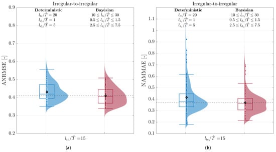
Figure 5. ANRMSE (a) and NAMMAE (b) box–violin plots. Comparison between deterministic and Bayesian predictions over the test sequences.

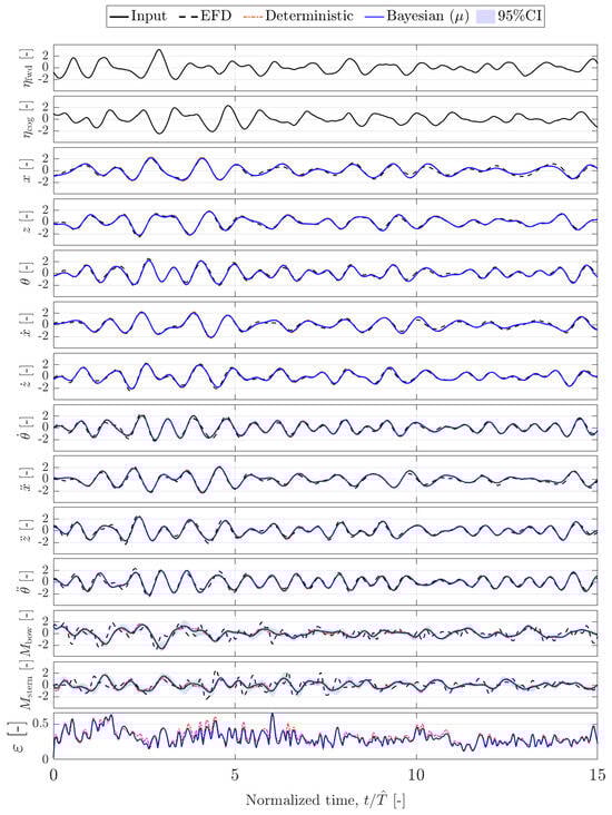
Figure 6. Standardized time series prediction by deterministic and Bayesian Hankel-DMDc. Irregular test wave, selected sequence 1.

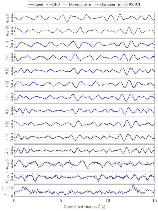
Figure 7. Standardized time series prediction by deterministic and Bayesian Hankel-DMDc. Irregular test wave, selected sequence 2.

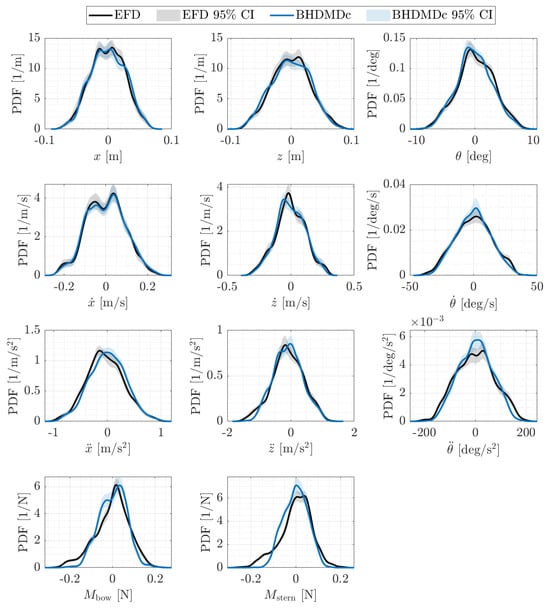
Figure 8. PDF comparison between measured data and Bayesian Hankel-DMDc prediction on bootstrapped sequences for each variable. Shaded areas indicate the 95% confidence interval of the two PDFs.

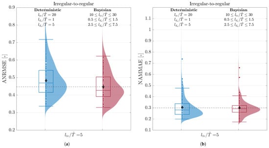
Figure 9. ANRMSE (a) and NAMMAE (b) box–violin plots. Comparison between deterministic and Bayesian predictions over the regular waves test sequences.

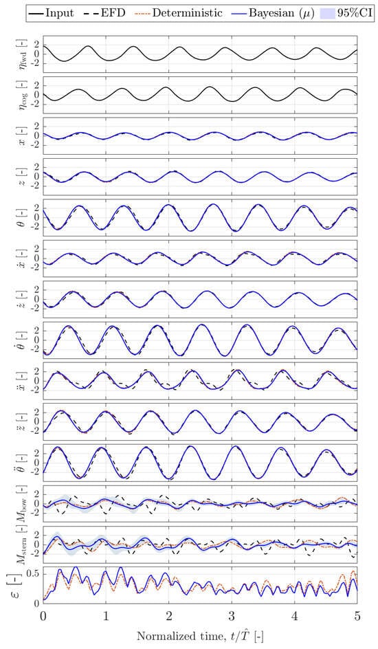
Figure 10. Standardized time series prediction by deterministic and Bayesian Hankel-DMDc. Regular test wave ${\lambda }_w/L_m=1.5$. Note that $\widehat{T}$ is evaluated from irregular waves.

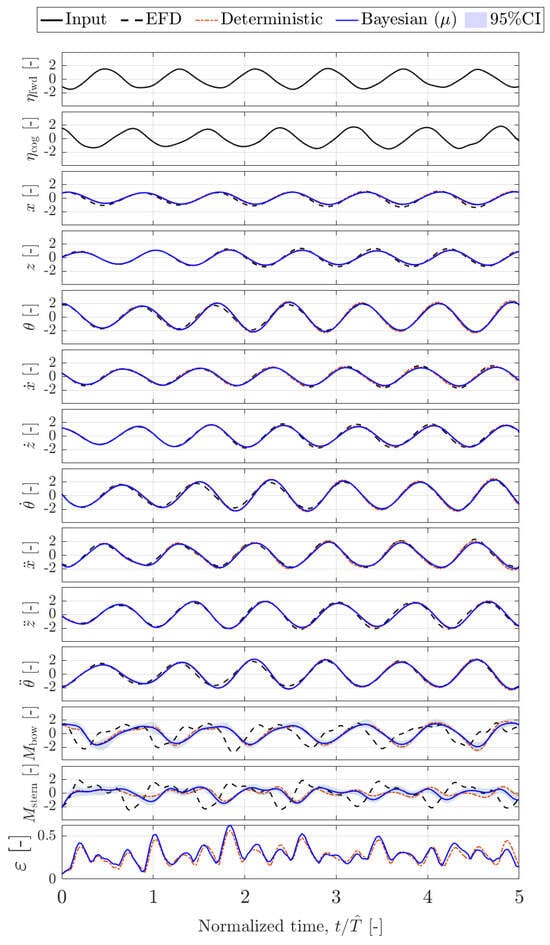
Figure 11. Standardized time series prediction by deterministic and Bayesian Hankel-DMDc. Regular test wave ${\lambda }_w/L_m=2$. Note that $\widehat{T}$ is evaluated from irregular waves.

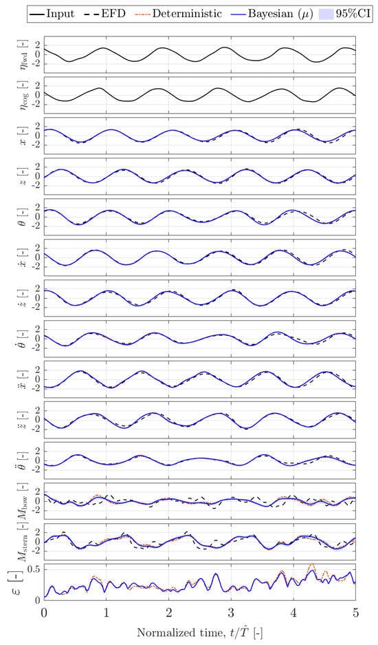
Figure 12. Standardized time series prediction by deterministic and Bayesian Hankel-DMDc. Regular test wave ${\lambda }_w/L_m=3$. Note that $\widehat{T}$ is evaluated from irregular waves.

In order to statistically assess the performance of HDMDc and BHDMDc, the ANRMSE and NAMMAE were evaluated for several training and testing sequences. In particular, 10 training sequences and 10 test sequences were randomly selected and combined in a full-factorial analysis. The same training and test sequences were used for the deterministic and Bayesian versions of the ROM to guarantee a fair comparison. The length of the test time histories for the irregular waves case was $l_{te}=15\widehat{T}$. Due to reduced signal lengths, $l_{te}=5\widehat{T}$ for regular waves.

For both irregular-to-irregular and irregular-to-regular cases, results are presented as box–violin plots comparing the ANRMSE and NAMMAE for the deterministic and Bayesian ROMs, see Figure 5 and Figure 9, respectively.

The boxes show the first, second (equivalent to the median value), and third quartiles, while the whiskers extend from the box to the farthest data point lying within 1.5 times the interquartile range, defined as the difference between the third and the first quartiles from the box. The density of the data distribution is additionally represented by the violin shape, providing a visual summary of the distribution beyond the quartiles. The values of single realizations, including outliers, are plotted with dots.

In addition, representative test sequences are shown in Figure 6 and Figure 7 for irregular-to-irregular and in Figure 10, Figure 11 and Figure 12 for irregular-to-regular cases. Figures compare the experimental measurements (EFD), the deterministic ROM prediction, and the Bayesian ROM prediction (mean value as solid line and 95% confidence interval as shaded area of the same color).

Finally, the MBB analysis is applied to the irregular-to-irregular case, and PDFs from bootstrapped sequences for EFD and BHDMDc are obtained for each predicted variable, along with their 95% confidence interval, and are shown in Figure 8. The differences between the EFD and BHDMDc distributions are evaluated using JSD, and results are summarized in Table 2.

Table 2. EV and 95% confidence lower bound, upper bound, and interval of JSD of the PDFs of variables in the bootstrapped time series.

JSDξ
Variable	EV	q = 0.025	q = 0.975	U
x	0.0026	0.0010	0.0061	0.0052
z	0.0031	0.0013	0.0061	0.0049
$\theta$	0.0035	0.0017	0.0076	0.0059
$\dot{x}$	0.0021	0.0007	0.0063	0.0057
$\dot{z}$	0.0036	0.0015	0.0075	0.0060
$\dot{\theta }$	0.0041	0.0011	0.0106	0.0095
$\ddot{x}$	0.0045	0.0028	0.0073	0.0045
$\ddot{z}$	0.0071	0.0030	0.0140	0.0110
$\ddot{\theta }$	0.0086	0.0028	0.0181	0.0153
$M_{\mathrm{bow}}$	0.0186	0.0099	0.0302	0.0203
$M_{\mathrm{stern}}$	0.0274	0.0185	0.0387	0.0202
avg	0.0077	0.0040	0.0139	0.0099

6.1. Irregular-to-Irregular

The HDMDc and the BHDMDc ROMs produce an overall reliable and robust prediction for unseen irregular input waves. No trend in $\epsilon \left(t\right)$ was observed throughout the testing window, suggesting that the same level of accuracy shown in $t\le 15\widehat{T}$ can be achieved for arbitrarily long sequences.

Observing the time-resolved predictions in Figure 6 and Figure 7 evidences that the great majority of the ANRMSE and NAMMAE errors arise from the prediction of the mooring forces. This is also confirmed by Table 2 showing that the JSD for the $M_{bow}$ e $M_{stern}$ PDFs is an order of magnitude higher than the other variables. Comparing the box–violin plot in Figure 5, it can be noted that the BHDMDc model reduced both ANRMSE and NAMMAE errors, lowering the average error and also reducing the results dispersion.

The uncertainty in the Bayesian model is very low, as can be observed in Figure 6 and Figure 7. This is consistent with the high accuracy achieved for vessel dynamics predictions and indicates the robustness of the model to hyperparameter changes in the identified ranges (confirming the rule of thumbs for the hyperparameter values identified in the literature [31,32]). However, confidence intervals are not sufficiently extended to cover the ground truth for mooring loads, whose predictions are less accurate and larger uncertainties would have been expected.

The remarkable accuracy obtained for the ship dynamics is also reflected in the MBB analysis, as the PDFs from EFD and BHDMDc data are very close, and their confidence intervals are almost always overlapping. The MBB analysis also confirms a reduced accuracy in the estimation of mooring forces.

The difficulty in obtaining accurate predictions of mooring forces is due to a combination of measurement noise and artifacts arising from the physical behavior of the mooring lines. Specifically, the mooring lines rested at the water surface, alternately emerging or being submerged by waves (particularly the bow mooring line), which induced sudden variations in tension that do not necessarily reflect the system dynamics. In addition, insufficient pretensioning, mainly due to an initial underestimation of the ASV mass and wave forces, caused the lines to be slack at times, further contributing to spurious oscillations in both the mooring lines and the measured loads. These factors complicated the learning of the system response by the DMD-based system identification, with a consequent increased error in the prediction of the mooring forces.

Nevertheless, the DMD-based models capture the low-frequency content of the loads, as can be seen in Figure 6 and Figure 7, achieving a fair estimation of load peaks. Regularization plays a key role, preventing the identification of spurious and unstable dynamics, to which the method is particularly sensitive in noisy data environments.

6.2. Irregular-to-Regular

The ROM learned in irregular wave conditions is tested in regular waves. Figure 10, Figure 11 and Figure 12 show the results of a selected test sequence for ${\lambda }_w=1.5L_m$, $2L_m$, and ${\lambda }_w=3L_m$, respectively. The DMD-based models achieve remarkable accuracy also in these cases for the variables linked to the ship’s dynamics, with the largest error being in the reproduction of mooring forces. Part of the error clearly arises from an imperfect identification of the load-related subsystem, already noted in the irregular waves data results. In addition, it has been noted that the issue evidenced for the measure of mooring forces was even more prominent in the regular waves case. During the regular wave tests, the model was more effectively pushed downstream by the regular waves from excitations with shorter wavelength, amplifying slackness of the stern line (loads on the stern mooring are consequently better predicted for higher ${\lambda }_w$).

The box–violin plots showing the statistical analysis of ANRMSE and NAMMAE results are presented in Figure 9. It can be noted that the ANRMSE is slightly higher than for irregular-to-irregular wave predictions; however, the NAMMAE is lower. This is coherent with a more pronounced phase error in the prediction of $M_{\mathrm{bow}}$ and $M_{\mathrm{stern}}$, while the models still provide a reasonable prediction of the loads’ extrema.

The ROMs trained on P-M irregular waves were able to predict vessel responses to regular head waves accurately. On one side, the regular wave frequencies lie in the decreasing side of the spectral peak of the training sea state $f\left({\lambda }_w=1.5L_m\right)=0.86$ Hz, $f\left({\lambda }_w=2L_m\right)=0.75$ Hz, and $f\left({\lambda }_w=3L_m\right)=0.61$ Hz, as can be seen from Figure 2. However, irregular and regular wave excitations have substantial differences in terms of frequency content and phase coherence. The successful prediction of regular-wave responses is, hence, an indication that the models have generalized beyond the specific type of excitation seen during training, at least when the new excitation remains within the spectral band covered during training. This highlights the importance of selecting informative training datasets, i.e., constructing and using training datasets that encompass a sufficiently rich representation of the system dynamics, enabling the development of ROMs capable of generalizing across multiple operating conditions. In this sense, irregular sea states appear promising due to their broadband spectral content, inherently providing a more comprehensive excitation of the system.

7. Conclusions

This work presented the system identification of a small ASV in moored conditions using the HDMDc and its uncertainty-aware extension, BHDMDc. The methods were applied to experimental data collected in the CNR-INM towing tank under both irregular and regular head wave conditions. The ASV under investigation features a recessed moon pool, which induces nonlinear responses due to sloshing, thereby increasing the modeling challenge.

The deterministic HDMDc formulation successfully captured the dominant dynamics of the vessel motions, providing accurate predictions of surge, heave, and pitch across all tested conditions. The prediction of mooring forces was more challenging and exhibited larger errors, mainly due to measurement noise and extremely nonlinear effects related to the partial slackening and intermittent immersion of the mooring lines. Nevertheless, the models were able to reproduce the low-frequency components and general trends of the mooring loads, offering a meaningful approximation of their temporal evolution.

The Bayesian extension introduced uncertainty quantification by propagating the variability of the HDMDc hyperparameters through Monte Carlo sampling. The Bayesian model consistently improved prediction accuracy compared to the deterministic version, also improving the robustness as measured by ANRMSE and NAMMAE.

A key outcome of this study is the generalization capability of HDMDc and BHDMDc models trained exclusively on irregular wave data. The trained models were able to accurately predict the ASV response in regular wave conditions, a different excitation regime although still characterized by frequencies within the spectral range of the training sea state. This highlights the importance of constructing informative training datasets that encompass a sufficiently rich system dynamics. In particular, irregular sea states, due to their broadband spectral content, inherently provide a more comprehensive excitation of the system, enabling the development of ROMs capable of generalizing across multiple operating conditions within the same frequency band. Further extending the approach to include, e.g., different sea states, wave directions, and operating conditions, would represent a key enabling technology for digital twins of marine systems, where reliable real-time predictions and uncertainty quantification are essential for control, monitoring, and decision support applications. In this context, the interpolation of parametric reduced-order models [52,53] may represent a viable strategy to overcome the intrinsic limitations of using a single, albeit informative, training set, by combining multiple locally trained models to construct a global predictive model that retains accuracy across a broader range of operating conditions.

References

- Serani, A.; Diez, M.; van Walree, F.; Stern, F. URANS analysis of a free-running destroyer sailing in irregular stern-quartering waves at sea state 7. Ocean Eng. 2021, 237, 109600. [Google Scholar] [CrossRef]
- Aram, S.; Mucha, P. CFD validation and analysis of turning maneuvers of a surface combatant in regular waves. Ocean Eng. 2024, 293, 116653. [Google Scholar] [CrossRef]
- Xu, W.; Maki, K.J.; Silva, K.M. A data-driven model for nonlinear marine dynamics. Ocean Eng. 2021, 236, 109469. [Google Scholar] [CrossRef]
- Yasukawa, H.; Yoshimura, Y. Introduction of MMG standard method for ship maneuvering predictions. J. Mar. Sci. Technol. 2015, 20, 37–52. [Google Scholar] [CrossRef]
- Yasukawa, H.; Hirata, N.; Nakayama, Y. High-Speed Ship Maneuverability. J. Ship Res. 2016, 60, 239–258. [Google Scholar] [CrossRef]
- Sanada, Y.; Park, S.; Kim, D.H.; Wang, Z.; Stern, F.; Yasukawa, H. Experimental and computational study of hull–propeller–rudder interaction for steady turning circles. Phys. Fluids 2021, 33, 127117. [Google Scholar] [CrossRef]
- Pandey, J.; Hasegawa, K. Manoeuvring mathematical model of catamaran wave adaptive modular vessel (WAM-V) using the system identification technique. In Proceedings of the 7th PAAMES and AMEC2016, Hong Kong, China, 13–14 October 2016; Volume 13, p. 14. [Google Scholar]
- Pandey, J.; Hasegawa, K. Study on Turning Manoeuvre of Catamaran Surface Vessel with a Combined Experimental and Simulation Method. In Proceedings of the 10th IFAC Conference on Control Applications in Marine Systems CAMS, Trondheim, Norway, 13–16 September 2016; Volume 49, pp. 446–451. [Google Scholar] [CrossRef]
- Diez, M.; Wang, Z.; Park, S.; Milano, C.; Stern, F.; Yasukawa, H.; Gunderson, A.; Scherer, J. Multi-Fidelity MMG-Model for Digital Design of High-Speed Small Craft. In Proceedings of the SNAME Chesapeake Power Boat Symposium, Norfolk, VA, USA, 14 October 2024; p. D011S002R003. [Google Scholar] [CrossRef]
- D’Agostino, D.; Serani, A.; Stern, F.; Diez, M. Time-series forecasting for ships maneuvering in waves via recurrent-type neural networks. J. Ocean Eng. Mar. Energy 2022, 8, 479–487. [Google Scholar] [CrossRef]
- Wang, N.; Kong, X.; Ren, B.; Hao, L.; Han, B. SeaBil: Self-attention-weighted ultrashort-term deep learning prediction of ship maneuvering motion. Ocean Eng. 2023, 287, 115890. [Google Scholar] [CrossRef]
- Jiang, Z.; Ma, Y.; Li, W. A Data-Driven Method for Ship Motion Forecast. J. Mar. Sci. Eng. 2024, 12, 291. [Google Scholar] [CrossRef]
- Diez, M.; Gaggero, M.; Serani, A. Data-driven forecasting of ship motions in waves using machine learning and dynamic mode decomposition. Int. J. Adapt. Control Signal Process. 2024, 39, 2119–2142. [Google Scholar] [CrossRef]
- Schmid, P.J. Dynamic mode decomposition of numerical and experimental data. J. Fluid Mech. 2010, 656, 5–28. [Google Scholar] [CrossRef]
- Kutz, J.; Brunton, S.; Brunton, B.; Proctor, J. Dynamic Mode Decomposition: Data-Driven Modeling of Complex Systems; SIAM—Society for Industrial and Applied Mathematics: Philadelphia, PA, USA, 2016. [Google Scholar] [CrossRef]
- Mezić, I. Koopman Operator, Geometry, and Learning of Dynamical Systems. Not. Am. Math. Soc. 2021, 68, 1087–1105. [Google Scholar] [CrossRef]
- Brunton, S.L.; Budišić, M.; Kaiser, E.; Kutz, J.N. Modern Koopman Theory for Dynamical Systems. SIAM Rev. 2022, 64, 229–340. [Google Scholar] [CrossRef]
- Koopman, B.O. Hamiltonian Systems and Transformation in Hilbert Space. Proc. Natl. Acad. Sci. USA 1931, 17, 315–318. [Google Scholar] [CrossRef]
- Proctor, J.L.; Brunton, S.L.; Kutz, J.N. Generalizing Koopman Theory to Allow for Inputs and Control. SIAM J. Appl. Dyn. Syst. 2018, 17, 909–930. [Google Scholar] [CrossRef]
- Rowley, C.W.; Mezić, I.; Bagheri, S.; Schlatter, P.; Hennigson, D.S. Spectral analysis of nonlinear flows. J. Fluid Mech. 2009, 641, 115–127. [Google Scholar] [CrossRef]
- Tang, Z.; Jiang, N. Dynamic mode decomposition of hairpin vortices generated by a hemisphere protuberance. Sci. China Phys. Mech. Astron. 2012, 55, 118–124. [Google Scholar] [CrossRef]
- Semeraro, O.; Bellani, G.; Lundell, F. Analysis of time-resolved PIV measurements of a confined turbulent jet using POD and Koopman modes. Exp. Fluids 2012, 53, 1203–1220. [Google Scholar] [CrossRef]
- Song, G.; Alizard, F.; Robinet, J.C.; Gloerfelt, X. Global and Koopman modes analysis of sound generation in mixing layers. Phys. Fluids 2013, 25, 124101. [Google Scholar] [CrossRef]
- Proctor, J.L.; Eckhoff, P.A. Discovering dynamic patterns from infectious disease data using dynamic mode decomposition. Int. Health 2015, 7, 139–145. [Google Scholar] [CrossRef]
- Brunton, B.W.; Johnson, L.A.; Ojemann, J.G.; Kutz, J.N. Extracting spatial–temporal coherent patterns in large-scale neural recordings using dynamic mode decomposition. J. Neurosci. Methods 2016, 258, 1–15. [Google Scholar] [CrossRef]
- Mann, J.; Kutz, J.N. Dynamic mode decomposition for financial trading strategies. Quant. Financ. 2016, 16, 1643–1655. [Google Scholar] [CrossRef]
- Diez, M.; Serani, A.; Campana, E.F.; Stern, F. Time-series forecasting of ships maneuvering in waves via dynamic mode decomposition. J. Ocean Eng. Mar. Energy 2022, 8, 471–478. [Google Scholar] [CrossRef]
- Serani, A.; Dragone, P.; Stern, F.; Diez, M. On the use of dynamic mode decomposition for time-series forecasting of ships operating in waves. Ocean Eng. 2023, 267, 113235. [Google Scholar] [CrossRef]
- Palma, G.; Serani, A.; Aram, S.; Wundrow, D.W.; Drazen, D.; Diez, M. Bayesian dynamic mode decomposition for real-time ship motion digital twinning. Appl. Ocean Res. 2025, 165, 104863. [Google Scholar] [CrossRef]
- Palma, G.; Serani, A.; Aram, S.; Wundrow, D.W.; Drazen, D.; Diez, M. Model-free system identification of surface ships in waves via Hankel dynamic mode decomposition with control. Ocean Eng. 2025, 341, 122539. [Google Scholar] [CrossRef]
- Palma, G.; Serani, A.; Diez, M.; Milano, C.; Wang, Z.; Park, S.; Sarigul, D.O.; Stern, F. Bayesian Hankel Extended Dynamic Mode Decomposition for System Identification of High-Speed Planing Hulls. In Proceedings of the International Conference on Fast Sea Technology (FAST), Norfolk, VA, USA, 29 October 2025. [Google Scholar]
- Palma, G.; Serani, A.; Diez, M. Data-driven uncertainty-aware seakeeping prediction of the Delft 372 catamaran using ensemble Hankel dynamic mode decomposition. J. Hydrodyn. 2025; under review. [Google Scholar]
- Takeishi, N.; Kawahara, Y.; Tabei, Y.; Yairi, T. Bayesian Dynamic Mode Decomposition. In Proceedings of the Twenty-Sixth International Joint Conference on Artificial Intelligence, IJCAI-17, Melbourne, Australia, 19–25 August 2017; pp. 2814–2821. [Google Scholar] [CrossRef]
- Sashidhar, D.; Kutz, J.N. Bagging, optimized dynamic mode decomposition for robust, stable forecasting with spatial and temporal uncertainty quantification. Philos. Trans. R. Soc. A Math. Phys. Eng. Sci. 2022, 380, 20210199. [Google Scholar] [CrossRef] [PubMed]
- Carter, D.J.T. Estimation of Wave Spectra from Wave Height and Period; Technical Report I.O.S. 135; Institute of Oceanographic Sciences: Wormley, UK, 1982. [Google Scholar]
- Schmid, P.; Sesterhenn, J. Dynamic Mode Decomposition of Numerical and Experimental Data. In Proceedings of the Sixty-First Annual Meeting of the APS Division of Fluid Dynamics, San Antonio, TX, USA, 23–25 November 2008. [Google Scholar]
- Proctor, J.L.; Brunton, S.L.; Kutz, J.N. Dynamic mode decomposition with control. SIAM J. Appl. Dyn. Syst. 2016, 15, 142–161. [Google Scholar] [CrossRef]
- Mezić, I. On Numerical Approximations of the Koopman Operator. Mathematics 2022, 10, 1180. [Google Scholar] [CrossRef]
- Otto, S.E.; Rowley, C.W. Linearly Recurrent Autoencoder Networks for Learning Dynamics. SIAM J. Appl. Dyn. Syst. 2019, 18, 558–593. [Google Scholar] [CrossRef]
- Takeishi, N.; Kawahara, Y.; Yairi, T. Learning Koopman invariant subspaces for dynamic mode decomposition. In Proceedings of the 31st International Conference on Neural Information Processing Systems, Red Hook, NY, USA, 4–9 December 2017; NIPS’17. pp. 1130–1140. [Google Scholar]
- Lusch, B.; Kutz, J.N.; Brunton, S.L. Deep learning for universal linear embeddings of nonlinear dynamics. Nat. Commun. 2018, 9, 4950. [Google Scholar] [CrossRef]
- Brunton, S.L.; Brunton, B.W.; Proctor, J.L.; Kutz, J.N. Koopman Invariant Subspaces and Finite Linear Representations of Nonlinear Dynamical Systems for Control. PLoS ONE 2016, 11, e0150171. [Google Scholar] [CrossRef] [PubMed]
- Arbabi, H.; Mezić, I. Ergodic Theory, Dynamic Mode Decomposition, and Computation of Spectral Properties of the Koopman Operator. SIAM J. Appl. Dyn. Syst. 2017, 16, 2096–2126. [Google Scholar] [CrossRef]
- Brunton, S.L.; Brunton, B.W.; Proctor, J.L.; Kaiser, E.; Kutz, J.N. Chaos as an intermittently forced linear system. Nat. Commun. 2017, 8, 19. [Google Scholar] [CrossRef]
- Xie, X.; Tang, S. Regularized dynamic mode decomposition algorithm for time sequence predictions. Theor. Appl. Mech. Lett. 2024, 14, 100555. [Google Scholar] [CrossRef]
- Marlantes, K.E.; Bandyk, P.J.; Maki, K.J. Predicting ship responses in different seaways using a generalizable force correcting machine learning method. Ocean Eng. 2024, 312, 119110. [Google Scholar] [CrossRef]
- Carlstein, E. The use of subseries values for estimating the variance of a general statistic from a stationary sequence. Ann. Stat. 1986, 14, 1171–1179. [Google Scholar] [CrossRef]
- Miecznikowski, J.C.; Wang, D.; Hutson, A. Bootstrap MISE Estimators to Obtain Bandwidth for Kernel Density Estimation. Commun. Stat. Simul. Comput. 2010, 39, 1455–1469. [Google Scholar] [CrossRef]
- Silverman, B.W. Density Estimation for Statistics and Data Analysis; Routledge: London, UK, 2018. [Google Scholar] [CrossRef]
- Lin, J. Divergence measures based on the Shannon entropy. IEEE Trans. Inf. Theory 1991, 37, 145–151. [Google Scholar] [CrossRef]
- Kullback, S.; Leibler, R.A. On Information and Sufficiency. Ann. Math. Stat. 1951, 22, 79–86. [Google Scholar] [CrossRef]
- Amsallem, D.; Farhat, C. Interpolation Method for Adapting Reduced-Order Models and Application to Aeroelasticity. AIAA J. 2008, 46, 1803–1813. [Google Scholar] [CrossRef]
- Amsallem, D.; Farhat, C. An Online Method for Interpolating Linear Parametric Reduced-Order Models. SIAM J. Sci. Comput. 2011, 33, 2169–2198. [Google Scholar] [CrossRef]
Disclaimer/Publisher’s Note: The statements, opinions and data contained in all publications are solely those of the individual author(s) and contributor(s) and not of MDPI and/or the editor(s). MDPI and/or the editor(s) disclaim responsibility for any injury to people or property resulting from any ideas, methods, instructions or products referred to in the content. |
© 2025 by the authors. Licensee MDPI, Basel, Switzerland. This article is an open access article distributed under the terms and conditions of the Creative Commons Attribution (CC BY) license (https://creativecommons.org/licenses/by/4.0/).