Formation Control of Autonomous Underwater Vehicles Using an Improved Nonlinear Backstepping Method

Abstract

The characteristics of autonomous underwater vehicles include nonlinearity, strong coupling, multiple inputs and multiple outputs, uncertainty, strong disturbance, underdrive, and multiple constraints. Autonomous underwater vehicle cluster systems are associated with large-scale complex dynamic systems through local perception or network communication, which have the structural characteristics of “complex dynamic + association topology + interaction rules”. To solve the problem of formation trajectory tracking of underactuated autonomous underwater vehicles, a controller was designed on the basis of an improved nonlinear backstepping algorithm, cascade system theory, and the Lyapunov direct method. In this design, the formation is determined from the actual trajectory of the leader autonomous underwater vehicle. The formation control rate is determined using the backstepping method and Lyapunov theory. Nonlinear disturbance observers were added to ensure that the trajectory error of the formation control could be quickly reduced in a real case with interference. The stability and effectiveness of this method were verified through simulation experiments. The robustness of the control algorithm was verified using two simulation cases, and the simulation results show that the proposed control method can maintain the expected formation.

1. Introduction

Autonomous underwater vehicle formations have great application potential. Compared to a single autonomous underwater vehicle (AUV), AUVs in formation have better environmental information perception ability and adaptability [1]. Commonly used formation control methods include the behavior-based method [2,3,4], the virtual structure method [5,6,7], the artificial potential field method [8,9,10] and the leader–follower method [11,12,13,14,15]. Kartal et al. [16] proposed a backstepping-based, distributed-formation control method that is stable and independent of time delays in communication among multiple unmanned aerial vehicles (UAVs). Liu et al. [17] presented a method for the cooperative formation control of a group of underactuated unmanned surface vessels (USVs). The followers must keep a fixed distance from the leader USV and a specific heading angle in order to maintain a certain type of formation. Dong et al. [18] presented a novel dynamic-surface sliding mode control (DSSMC) method, combined with a lateral velocity-tracking differentiator (LVTD), for the cooperative formation control of underactuated unmanned marine vehicles exposed to complex marine environment disturbances. Gu et al. [19] investigated the model-free containment control of multiple underactuated USVs subject to unknown kinetic models. Zhang et al. [20] presented a robust adaptive control approach for underactuated surface ship linear path-tracking control systems on the basis of the backstepping control method and Lyapunov stability theory. Fu et al. [21] presented a solution to the formation control problem for underactuated unmanned surface vehicles using a distributed strategy based on the virtual leader strategy. Qin et al. [22] investigated the trajectory-tracking control problem for USVs with input saturation and full-state constraints. Wang et al. [23] proposed filter-backstepping-based neural adaptive formation control of leader-following AUVs with model uncertainties and external disturbances in three-dimensional space. Wang et al. [24] presented a distributed formation-tracking control strategy that acts on multiple quadrotor unmanned aerial vehicle (QUAV) formation control under external disturbance and asymmetric output error constraints.

Yan et al. [25] designed a new formation structure based on graph theory and the virtual leader technique. This special structure fixes the connection between AUVs as a triangle formed by leads and neighborhood AUVs, thus increasing the stiffness and position accuracy of the structure and increasing the stability of the formation structure. Panagou and Kumar [11] proposed a robot cooperative-movement method under communication constraints in an environment with known obstacles, which does not require data interaction between the robots but allows them to each perform their respective tasks based on local information. Stover et al. [12] proposed a strategy in which the position of the follower is not strictly fixed relative to the leader’s position in the formation maintenance process, but appropriately changes based on the equidistant arc centered on the leader’s reference frame. Ji et al. [13] proposed a leader–follower hybrid control scheme based on stagnation rules. Once the leader reaches the ideal formation, the followers will converge into a convex polyhedron centered by the leader. When the required leader task fails, the leader will form a fixed formation with the same speed and direction. Thus, the followers converge at the same speed and direction as the leader. Due to the similar characteristics of multi-AUV systems and neural networks, some researchers have also tried to combine neural networks with formation control, and achieved good results. For example, Li and Zhu [14] proposed a Self-Organizing Map (SOM) neural network method for the distributed formation control of underwater robot clusters. It includes the special definition of the initial neural weights of the network, the selection rules of winners, the law of workload balance, the updating method of weights, and the formation-tracking strategy. Each AUV controller uses only its own information and the limited information of neighboring AUVs, without explicitly specifying leaders and followers, and all AUVs are considered leaders or followers, so they have better adaptability and fault tolerance. In view of formation control in complex scenarios where obstacles need to be avoided, Ding and Zhu et al. [15] adopted a bio-inspired neural network model to realize three-dimensional formation control and obstacle avoidance for AUVs. Each neuron in the neural network represents a step of the leader AUV, the leader AUV communication line is determined according to the output activity value of the neurons in the neural network, and the final navigation of the leader AUV is translated into the activity value of the neuron output in the neural network.

However, the functionality of current AUVs is insufficient to complete missions in complex situations. This paper presents an AUV formation controller based on the controller design method proposed by Wan et al. [26] using the cascade system and Lyapunov direct method.

The main contributions of this work are summarized as follows. Unlike traditional full-trajectory guidance, which uses the expected trajectory of the leader AUV for formation control, the proposed method adopts the actual trajectory of the leader autonomous underwater vehicle for formation control, which can make the formation situation closer to the actual situation. By using global differential homeomorphism transformation, the complex formation control system is decomposed into a cascaded system that is easier to analyze. A formation controller based on the nonlinear backstepping method was designed, and by combining Lyapunov stability theory with cascade system theory, it was proven that the entire formation control system is globally, uniformly, and asymptotically stable. In addition, a nonlinear disturbance observer was designed to address complex disturbances in actual marine environments, improving the anti-interference ability of the control algorithm. Finally, the effectiveness, stability, and reliability of the proposed control method were verified through simulation experiments.

The composition of the paper is as follows. In Section 2, the mathematical model and the problem is presented. In Section 3, the controller design is described, and its stability is analyzed in Section 4. A leader–follower formation consisting of three AUVs is verified using simulation results in Section 5. The conclusions and discussion are shown in Section 6.

2. Problem Description

2.1. Mathematical Model of an AUV

In this study, it was assumed that the formation consists of m + 1 AUVs, corresponding to a leader AUV and m follower AUVs. The kinematic model [27] of the ith AUV is

$${\dot{\eta }}_i=R\left({\phi }_i\right)v$$

(1)

where ${\eta }_i$ is a state vector for the AUV; ${\eta }_i={\left[x_i,y_i,{\phi }_i\right]}^T$, where $x_i$ is the portrait position, $y_i$ is the lateral position, and ${\phi }_i$ is the bow speed.

$R\left({\phi }_i\right)$ is the rotation matrix of the bow, defined as

$$R\left({\phi }_i\right)=\left(\begin{array}{ccc}\mathit{cos}{\phi }_i& -\mathit{sin}{\phi }_i& 0\\ \mathit{sin}{\phi }_i& \mathit{cos}{\phi }_i& 0\\ 0& 0& 1\end{array}\right)$$

The horizontal nonlinear dynamical model of the AUV is

$$M_i{v}_i+C\left(v_i\right)v_i+D\left(v_i\right)v_i={\tau }_i$$

(2)

where $M_i$ is the inertia coefficient matrix, $C_i$ is the Coriolis force and centripetal force matrix, and $D_i$ is the damping coefficient matrix. They are defined as

$$M_i=\left(\begin{array}{ccc}{m}_{1i}& 0& 0\\ 0& m_{2i}& 0\\ 0& 0& m_{3i}\end{array}\right),D(v_i)=\left(\begin{array}{ccc}{d}_{1i}& 0& 0\\ 0& d_{2i}& 0\\ 0& 0& d_{3i}\end{array}\right),C(v_i)=\left(\begin{array}{ccc}0& 0& -m_{2i}{v}_i\\ 0& 0& m_{1i}{u}_i\\ m_{2i}{v}_i& m_{1i}{u}_i& 0\end{array}\right)$$

$m_{1i}$, $m_{2i}$, and $m_{3i}$ are the combined terms of the AUV’s mass and additional mass; $d_{1i}$, $d_{2i}$, and $d_{3i}$ are hydrodynamic resistance.

The underactuated model of the AUV is

$$\left\{\begin{array}{l}{\dot{x}}_i=u\mathit{cos}{\phi }_i-v_i\mathit{sin}{\phi }_i\\ {\dot{y}}_i=u\mathit{sin}{\phi }_i+v_i\mathit{cos}{\phi }_i\\ {\dot{\phi }}_i=r_i\\ {\dot{u}}_i=\frac{m_{2i}}{m_{1i}}{v}_i{r}_i-\frac{d_{1i}}{m_{1i}}{u}_i+\frac{1}{m_{1i}}{\tau }_{ui}\\ {\dot{v}}_i=\frac{m_{1i}}{m_{2i}}{u}_i{r}_i-\frac{d_{2i}}{m_{2i}}{v}_i\\ {\dot{r}}_i=\frac{m_{1i}-m_{2i}}{m_{3i}}{u}_i{v}_i-\frac{d_{3i}}{m_{3i}}{r}_i+\frac{1}{m_{3i}}{\tau }_{ri}\end{array}\right.$$

(3)

2.2. AUV Formation Model

The mathematical model of the AUV formation based on the leader–follower method is shown in Figure 1. $\left(x_l,y_l\right),\left(x_f,y_f\right)$ is the actual trajectory position of the leader AUV and the follower AUVs in the geodetic coordinate system. ${\phi }_l,{\phi }_f$ is the actual trajectory heading angle of the leader AUV and follower AUVs, and $L,\theta \left(\theta \in \left(-\pi ,\pi \right)\right)$ is the distance and angle of the follower AUVs relative to the leader AUV. $l_x=L\mathit{cos}\theta \mathrm{a}\mathrm{n}\mathrm{d}{l}_y=L\mathit{sin}\theta$ are the decomposition of the distance and angle between the follower AUVs and the leader AUV in the leader AUV’s body-fixed coordinate system. $l_x$ and $l_y$are the relative longitudinal distance and lateral distance of a follower AUV in the follower AUV’s body-fixed coordinate system. $l_x=L\mathit{cos}\theta ,l_y=L\mathit{sin}\theta$ denote the decomposition of the distance L and angle θ between the follower AUVs and the leader AUV in the leader AUV’s body-fixed coordinate system. When the position and course information of the leader AUV are known, as long as $l_x,l_y$ are fixed, then the formation is also fixed. Therefore, by controlling the distance and angle $(L,\theta )$ between the two AUVs to achieve the desired formation, it can be transformed into the control of the longitudinal and lateral distance $l_x,l_y$ of the $i$th follower AUV relative to the leader AUV.

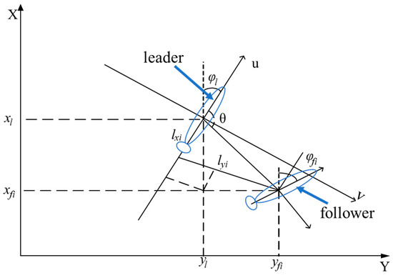
Figure 1. Leader–follower AUV formation model.

Figure 1 shows that the longitudinal distance, lateral distance, and course deviation of the $i$th follower AUV relative to the leader AUV are

$$\left\{\begin{array}{l}{l}_{xid}=(x_{fid}-x_l)\mathit{cos}{\phi }_l+(y_{fid}-y_l)\mathit{sin}{\phi }_l\\ l_{yid}=-(x_{fid}-x_l)\mathit{sin}{\phi }_l+(y_{fid}-y_l)\mathit{cos}{\phi }_l\\ {\phi }_{ied}={\phi }_{fid}-{\phi }_l\end{array}\right.$$

(4)

$$\left[\begin{array}{c}{x}_{fid}\\ y_{fid}\\ {\phi }_{fid}\end{array}\right]=\left[\begin{array}{ccc}\mathit{cos}{\phi }_l& -\mathit{sin}{\phi }_l& 0\\ \mathit{sin}{\phi }_l& \mathit{cos}{\phi }_l& 0\\ 0& 0& 1\end{array}\right]\left[\begin{array}{c}{l}_{xid}\\ \begin{array}{c}{l}_{yid}\\ {\phi }_{ied}\end{array}\end{array}\right]+\left[\begin{array}{c}{x}_l\\ \begin{array}{c}{y}_l\\ {\phi }_l\end{array}\end{array}\right]$$

(5)

Taking the derivative, this formula yields

$$\left[\begin{array}{c}{\dot{x}}_{fid}\\ {\dot{y}}_{fid}\\ {\dot{\phi }}_{fid}\end{array}\right]=\left[\begin{array}{ccc}-r_l\mathit{sin}{\phi }_l& -r_l\mathit{cos}{\phi }_l& 0\\ r_l\mathit{cos}{\phi }_l& -r_l\mathit{sin}{\phi }_l& 0\\ 0& 0& 0\end{array}\right]\left[\begin{array}{c}{l}_{xid}\\ \begin{array}{c}{l}_{yid}\\ {\phi }_{ied}\end{array}\end{array}\right]+\left[\begin{array}{c}{\dot{x}}_l\\ \begin{array}{c}{\dot{y}}_l\\ {\dot{\phi }}_l\end{array}\end{array}\right]$$

(6)

$$\left\{\begin{array}{l}{\dot{x}}_{fid}=-r_l\mathit{sin}{\phi }_l{l}_{xid}-r_l\mathit{cos}{\phi }_l{l}_{yid}+u_l\mathit{cos}{\phi }_l-v_l\mathit{sin}{\phi }_l\\ {\dot{y}}_{fid}=r_l\mathit{cos}{\phi }_l{l}_{xid}-r_l\mathit{sin}{\phi }_l{l}_{yid}+u_l\mathit{sin}{\phi }_l+v_l\mathit{cos}{\phi }_l\\ {\dot{\phi }}_{fid}={\dot{\phi }}_l\end{array}\right.$$

which can be rewritten as

$$\left\{\begin{array}{l}{\phi }_{fid}=ac\mathit{tan}2({\dot{y}}_{fid},{\dot{x}}_{fid})\\ u_{fid}={\dot{x}}_{fid}\mathit{cos}{\phi }_{fid}+{\dot{y}}_{fid}\mathit{sin}{\phi }_{fid}\\ r_{fid}={\dot{\phi }}_l=r_l\\ {\dot{v}}_{fid}=-\frac{m_{11}}{m_{22}}{u}_{fid}{r}_{fid}-\frac{d_{22}}{m_{22}}{v}_{fid}\end{array}\right.$$

(7)

Unlike the traditional full-trajectory guidance, which uses the expected trajectory of the leader AUV for formation control, the proposed method adopts the actual trajectory of the leader AUV for formation control, which can bring the formation situation closer to the actual situation.

3. Controller Design

3.1. Global Differential Homeomorphism Transformation

The differential homeomorphism intermediate-state variable of the $i$th AUV is designed as

$$\left\{\begin{array}{l}{\alpha }_{1i}=x_i\mathit{cos}{\phi }_i-y_i\mathit{sin}{\phi }_i\\ {\alpha }_{2i}=-x_i\mathit{sin}{\phi }_i+y_i\mathit{cos}{\phi }_i+\frac{m_{22}}{d_{22}}{v}_i\\ {\alpha }_{3i}={\phi }_i\\ {\alpha }_{4i}=-\frac{m_{11}}{d_{22}}{u}_i-x_i\mathit{cos}{\phi }_i-y_i\mathit{sin}{\phi }_i\\ {\alpha }_{5i}=v_i\\ {\alpha }_{6i}=r_i\end{array}\right.$$

(8)

Taking the derivative of Formula (8) yields the results of the derivation, as shown in Appendix A.

Realizing a stabilizing control system requires a feedback design for the input ($F_i,N_i$):

$$\left\{\begin{array}{l}{f}_{1i}=-\frac{m_{11}}{d_{22}}{\dot{u}}_i+\frac{d_{22}}{m_{11}}({\alpha }_{1i}+{\alpha }_{4i})-{\alpha }_{2i}{\alpha }_{6i}+\frac{m_{22}}{d_{22}}{\alpha }_{5i}{\alpha }_{6i}\\ f_{2i}={\dot{r}}_i\end{array}\right.$$

(9)

According to the design of the foregoing intermediate variable and derivative analysis, the mathematical equations of motion for the ith follower AUV are

$$\left\{\begin{array}{l}{\dot{\alpha }}_{1i}=-\frac{d_{22}}{m_{11}}{\alpha }_{1i}-\frac{d_{22}}{m_{11}}{\alpha }_{4i}+{\alpha }_{2i}{\alpha }_{6i}-\frac{m_{22}}{d_{22}}{\alpha }_{5i}{\alpha }_{6i}\\ {\dot{\alpha }}_{2i}={\alpha }_{4i}{\alpha }_{6i}\\ {\dot{\alpha }}_{3i}={\alpha }_{6i}\\ {\dot{\alpha }}_{4i}=f_{1i}\\ {\dot{\alpha }}_{5i}=\frac{d_{22}}{m_{22}}({\alpha }_{1i}+{\alpha }_{4i}){\alpha }_{6i}-\frac{d_{22}}{m_{22}}{\alpha }_{5i}\\ {\dot{\alpha }}_{6i}=f_{2i}\end{array}\right.$$

(10)

Through a global differential homeomorphism transformation, every variable ${\alpha }_{ni}$ can be converged to zero in an overall situation by using ($f_{1i},f_{2i}$), n = 1, 2, … The state of the reference trajectory for the ith follower AUV $[x_{id},y_{id},{\phi }_{id},u_{id},v_{id},r_{id}]$ can also be converted to $f_{1id},f_{2id}$, ${\alpha }_{nid}$ via the global differential homeomorphism transformation $f_{1id},f_{2id}$, ${\alpha }_{nid}$, n = 1, 2, …, and this expression is

$$\left\{\begin{array}{l}{\dot{\alpha }}_{1id}=-\frac{d_{22}}{m_{11}}{\alpha }_{1id}-\frac{d_{22}}{m_{11}}{\alpha }_{4id}+{\alpha }_{2id}{\alpha }_{6id}-\frac{m_{22}}{d_{22}}{\alpha }_{5id}{\alpha }_{6id}\\ {\dot{\alpha }}_{2id}={\alpha }_{4id}{\alpha }_{6id}\\ {\dot{\alpha }}_{3id}={\alpha }_{6id}\\ {\dot{\alpha }}_{4id}=f_{1id}\\ {\dot{\alpha }}_{5id}=\frac{d_{22}}{m_{22}}({\alpha }_{4id}+{\alpha }_{1id}){\alpha }_{6id}-\frac{d_{22}}{m_{22}}{\alpha }_{5id}\\ {\dot{\alpha }}_{6id}=f_{2id}\end{array}\right.$$

(11)

where $f_{1id},f_{2id}$ are

$$\left\{\begin{array}{l}{f}_{1id}=-\frac{m_{11}}{d_{22}}{\dot{u}}_{id}+\frac{d_{22}}{m_{11}}({\alpha }_{1id}+{\alpha }_{4id})-{\alpha }_{2id}{\alpha }_{6id}+\frac{m_{22}}{d_{22}}{\alpha }_{5id}{\alpha }_{6id}\\ f_{2id}={\dot{r}}_{id}\end{array}\right.$$

(12)

The error of the ith follower AUV is

$$e={\alpha }_{ni}-{\alpha }_{nid},n=\mathrm{1,2},...$$

(13)

$$\left\{\begin{array}{c}{\dot{e}}_{1i}=-\frac{d_{22}}{m_{11}}{e}_{1i}-\frac{d_{22}}{m_{11}}{e}_{4i}+(e_{2i}{e}_{6i}+e_{4i}{\alpha }_{6id}+e_{6i}{\alpha }_{2id})\\ -\frac{m_{22}}{d_{22}}(e_{5i}{e}_{6i}+e_{5i}{\alpha }_{6id}+e_{6i}{\alpha }_{5id})\\ {\dot{e}}_{2i}=e_{4i}{e}_{6i}+e_{4i}{\alpha }_{6id}+e_{6i}{\alpha }_{5id}\\ {\dot{e}}_{3i}=e_{6i}\\ {\dot{e}}_{4i}=f_{1i}-f_{1id}\\ {\dot{e}}_{5i}=\frac{d_{22}}{m_{22}}(e_{4i}{e}_{6i}+e_{4i}{\alpha }_{6id}+e_{6i}{\alpha }_{4id}+e_{1i}{e}_{6i}+e_{1i}{\alpha }_{6id}+e_{6i}{\alpha }_{1id})\\ -\frac{d_{22}}{m_{22}}{e}_{5i}\\ {\dot{e}}_{6i}=f_{2i}-f_{2id}\end{array}\right.$$

(14)

Then, the formation error shown in Formula (14) can be decomposed into a cascade system:

$$\left[\begin{array}{c}{\dot{e}}_{1i}\\ {\dot{e}}_{2i}\\ {\dot{e}}_{4i}\\ {\dot{e}}_{5i}\end{array}\right]=\left[\begin{array}{c}-\frac{d_{22}}{m_{11}}{e}_{1i}-\frac{d_{22}}{m_{11}}{e}_{4i}+e_{2i}{\alpha }_{6id}-\frac{m_{22}}{d_{22}}{e}_{5i}{\alpha }_{6id}\\ e_{4i}{\alpha }_{6id}\\ f_{1i}-f_{1id}\\ -\frac{d_{22}}{m_{22}}{e}_{5i}+\frac{d_{22}}{m_{22}}(e_{4i}{\alpha }_{6id}+e_{1i}{\alpha }_{6id})\end{array}\right]+\left[\begin{array}{c}0\\ 0\\ 0\\ 0\end{array}\right.\left.\begin{array}{c}-\frac{m_{22}}{d_{22}}(e_{5i}+{\alpha }_{5id})\\ e_{4i}+{\alpha }_{4id}\\ 0\\ \frac{d_{22}}{m_{22}}(e_{4i}+{\alpha }_{4id}+e_{1i}+{\alpha }_{1id})\end{array}\right]\left[\begin{array}{c}{e}_{3i}\\ e_{6i}\end{array}\right]$$

(15)

$$\left[\begin{array}{c}{\dot{e}}_{3i}\\ {\dot{e}}_{6i}\end{array}\right]=\left[\begin{array}{c}{e}_{6i}\\ f_{2i}-f_{2id}\end{array}\right]$$

(16)

So far, the formation error model guided by the actual trajectory has been transformed into a formation error cascade system. The formation control of AUVs based on the leader–follower method can be transformed into a trajectory-tracking control problem of the formation; then, the formation error system is finally decomposed into a cascade system that is easy to analyze through the global differential homeomorphism transformation. Finally, the problem is simplified into a stabilization problem of the trajectory-tracking error state of each autonomous underwater vehicle.

3.2. Backstepping Controller Design

From the cascading system of Formula (15),

$$\left[\begin{array}{c}{\dot{e}}_{1i}\\ {\dot{e}}_{2i}\\ {\dot{e}}_{4i}\\ {\dot{e}}_{5i}\end{array}\right]=\left[\begin{array}{c}-\frac{d_{22}}{m_{11}}{e}_{1i}-\frac{d_{22}}{m_{11}}{e}_{4i}+e_{2i}{\alpha }_{6id}-\frac{m_{22}}{d_{22}}{e}_{5i}{\alpha }_{6id}\\ e_{4i}{\alpha }_{6id}\\ f_{1i}-f_{1id}\\ -\frac{d_{22}}{m_{22}}{e}_{5i}+\frac{d_{22}}{m_{22}}(e_{4i}{\alpha }_{6id}+e_{1i}{\alpha }_{6id})\end{array}\right]$$

(17)

Let $e_{4i}$ be the input of the system of Formula (17); its virtual quantity is defined according to the design principle of the nonlinear backstepping method as ${\tilde{e}}_{4i}$:

$${\tilde{e}}_{4i}=k_{1i}{e}_{1i}-k_{2i}{\alpha }_{6id}{e}_{2i}-k_{3i}{\alpha }_{6id}{e}_{5i}$$

(18)

All values of $k_{1i},k_{2i},k_{3i}$ are greater than zero.

Then, the error ${\Delta }_i$ between the virtual input ${\tilde{e}}_{4i}$ and the actual input $e_{4i}$ is defined as

$${\Delta }_i=e_{4i}-{\tilde{e}}_{4i}$$

(19)

Taking its derivative yields

$$\begin{array}{cc}\hfill {\dot{\Delta }}_i& ={\dot{e}}_{4i}-{\dot{\tilde{e}}}_{4i}\hfill \\ & =f_{1i}-f_{1id}-(k_{1i}{\dot{e}}_{1i}-k_{2i}{\dot{\alpha }}_{6id}{e}_{2i}-k_{2i}{\alpha }_{6id}{\dot{e}}_{2i}\hfill \\ & -k_3{\dot{\alpha }}_{6id}{e}_{5i}-k_{3i}{\alpha }_{6id}{\dot{e}}_{5i})\hfill \end{array}$$

(20)

Bringing the result into the system of Formula (15) yields a new cascading error system:

$$\left\{\begin{array}{l}{\dot{e}}_{1i}=-\frac{d_{22}}{m_{11}}(1+k_{1i})e_{1i}+(\frac{d_{22}}{m_{11}}{k}_{2i}+1)e_{2i}{\alpha }_{6id}+(\frac{d_{22}}{m_{11}}{k}_{3i}-\frac{m_{22}}{d_{22}})e_{5i}{\alpha }_{6id}-\frac{d_{22}}{m_{11}}{\Delta }_i\\ {\dot{e}}_{2i}=-k_{2i}{\alpha }_{6id}^2{e}_{2i}+k_{1i}{\alpha }_{6id}{e}_{1i}-k_{3i}{\alpha }_{6id}^2{e}_{5i}+{\alpha }_{6id}{\Delta }_i\\ {\dot{\Delta }}_i=f_{1i}-f_{1id}-(k_{1i}{\dot{e}}_{1i}-k_{2i}{\dot{\alpha }}_{6id}{e}_{2i}-k_{2i}{\alpha }_{6id}{\dot{e}}_{2i}-k_{3i}{\dot{\alpha }}_{6id}{e}_{5i})\\ {\dot{e}}_{5i}=-\frac{d_{22}}{m_{22}}(1+k_{3i}{\alpha }_{6id}^2)e_{5i}+\frac{d_{22}}{m_{22}}(1+k_{1i})e_{1i}{\alpha }_{6id}-\frac{d_{22}}{m_{22}}{k}_{2i}{\alpha }_{6id}^2{e}_{2i}+\frac{d_{22}}{m_{22}}{\alpha }_{6id}{\Delta }_i\end{array}\right.$$

(21)

The Lyapunov function of the system of Formula (21) is

$$V_{1i}=\frac{1}{2}{\lambda }_{1i}{e}_{1i}^2+\frac{1}{2}{\lambda }_{2i}{e}_{2i}^2+\frac{1}{2}{\Delta }_i^2+\frac{1}{2}{\lambda }_{3i}{e}_{5i}^2$$

(22)

where the values of ${\lambda }_{1i},{\lambda }_{2i},{\lambda }_{3i}$ are greater than zero. Taking the derivative of Formula (22), according to Formula (21), we can design the control rate $f_{1i}$ as

$$\begin{array}{cc}\hfill f_{1i}& =f_{1id}+(k_{1i}{\dot{e}}_{1i}-k_{2i}{\dot{\alpha }}_{6id}{e}_{2i}-k_{2i}{\alpha }_{6id}{\dot{e}}_{2i}-k_{3i}{\dot{\alpha }}_{6id}{e}_{5i}-k_{3i}{\alpha }_{6id}{\dot{e}}_{5i})\hfill \\ & +\frac{{\lambda }_{1i}{d}_{22}}{m_{11}}{e}_{1i}-{\lambda }_{2i}{\alpha }_{6id}{e}_{2i}-\frac{{\lambda }_{3i}{d}_{22}}{m_{22}}{\alpha }_{6id}{e}_{5i}-k_{4i}{\Delta }_i\hfill \end{array}$$

(23)

where $k_{4i}$ is a positive number. Similarly, from the system of Formula (16),

$$\left[\begin{array}{c}{\dot{e}}_{3i}\\ {\dot{e}}_{6i}\end{array}\right]=\left[\begin{array}{c}{e}_{6i}\\ f_{2i}-f_{2id}\end{array}\right]$$

(24)

Let $e_{6i}$ be the input of the system of Formula (16). Its virtual quantity ${\tilde{e}}_{6i}$ is defined according to the design principle of the nonlinear backstepping method:

$${\tilde{e}}_{6i}=-k_{5i}{e}_{3i}$$

(25)

where $k_{5i}$ is a positive number. Then, the error ${\sigma }_i$ between the virtual input ${\tilde{e}}_{6i}$ and the actual input $e_{6i}$ is defined as

$${\sigma }_i=e_{6i}-{\tilde{e}}_{6i}$$

(26)

Taking its derivative yields.

The new cascading error systems are available:

$$\left\{\begin{array}{l}{\dot{e}}_{3i}={\sigma }_i-k_{5i}{e}_{3i}\\ {\dot{\sigma }}_i={\dot{e}}_{6i}-{\dot{\tilde{e}}}_{6i}=f_{2i}-f_{2id}-{\dot{\tilde{e}}}_{6i}\end{array}\right.$$

(27)

The Lyapunov function $V_{2i}$ of the system of Formula (27) is

$$V_{2i}=\frac{1}{2}{k}_{6i}{e}_{3i}^2+\frac{1}{2}{\sigma }_i^2$$

(28)

where $k_{6i}$ is a positive number. Taking the derivative of Formula (28) yields

$$\begin{array}{cc}\hfill {\dot{V}}_{2i}& =k_{6i}{e}_{3i}{\dot{e}}_{3i}+{\sigma }_i{\dot{\sigma }}_i\hfill \\ & =k_{6i}{e}_{3i}({\sigma }_i-k_{5i}{e}_{3i})+{\sigma }_i(f_{2i}-f_{2id}-{\dot{\tilde{e}}}_{6i})\hfill \\ & =-k_{5i}{k}_{6i}{e}_{3i}^2+{\sigma }_i(f_{2i}-f_{2id}-{\dot{\tilde{e}}}_{6i}+k_{6i}{e}_{3i})\hfill \end{array}$$

(29)

From Formula (29), we can design the control rate $f_{2i}$:

$$\begin{array}{cc}\hfill f_{2i}& =-k_{7i}{\sigma }_i+f_{2id}+{\dot{\tilde{e}}}_{6i}-k_{6i}{e}_{3i}\hfill \\ & =-k_{7i}({\sigma }_i+k_{5i}{e}_{3i})-k_{5i}{\dot{e}}_{3i}-k_{6i}{e}_{3i}+f_{2id}\hfill \\ & =-k_{7i}{\sigma }_i-(k_{6i}+k_{7i}{k}_{5i})e_{3i}-k_{5i}{\dot{e}}_{3i}+f_{2id}\hfill \end{array}$$

(30)

where $k_{7i}$ is a positive number.

3.3. Design of the Nonlinear Interference Observer

Here, we can use the standard Cauchy form:

$$\left\{\begin{array}{l}{\dot{x}}_1=x_2\\ {\dot{x}}_2=f+gU+d\end{array}\right.$$

(31)

where U is the control quantity and d is the interference. Without considering the interference d, the ideal differential equations for the system can be obtained:

$$\left\{\begin{array}{l}{\dot{x}}_1=x_2\\ {\dot{x}}_2=f+gU\end{array}\right.$$

(32)

We can then design the interference observer as

$$\dot{z}=-Lz-L(L{x}_2+f+gU)\widehat{d}=z+L{x}_2$$

(33)

Using Formula (33) to obtain an estimate $\widehat{d}$ of the interference and bringing it into the system to eliminate it enables the system to be compensated, so as to approach the ideal system of Formula (32).

4. Stability Analysis

4.1. Proving the Stability of the Backstepping Method

The two lemmas required for the proof process are given as follows.

Lemma 1.

Given the following nonlinear cascade system [28],

$$\left\{\begin{array}{l}\dot{x}=f_1(t,x)+g(t,x,y)y\\ \dot{y}=f_2(t,y)\end{array}\right.$$

(34)

$x\in R^n,y\in R^m$, and $f_1(t,x)$ are continuously differentiable in $(t,x)$. $f_2(t,y)$ and $g(t,x,y)$ are continuous functions. Taking the local $Lipschitz$ for $y$ and $(x,y)$ at the same time enables the conversion of the system of Formula (34) to

$$\dot{x}=f_1(t,x)$$

(35)

and its interference system

$$\dot{y}=f_2(t,y)$$

(36)

When the system of Formula (36) stabilizes toward to zero, the stability of the system of Formula (34) is related only to that of the system of Formula (35). When the following conditions are satisfied, the system of Formula (34) is consistent and progressively stable in the overall situation:

Condition 1.

The subsystem (Formula (35)) of the system of Formula (34) is consistent and asymptotically stable in the overall situation, and there are continuously differentiable functions $V(t,x):R\ge 0\times R^n\to R$ that meet this condition:

$$\left\{\begin{array}{l}W\left(x\right)\le V(t,x)\\ \frac{\partial V}{\partial t}+\frac{\partial V}{\partial x}\cdot f_1(t,x)\le 0,\forall ‖x‖\ge \eta \\ ‖\frac{\partial V}{\partial x}‖‖x‖\le cV(t,x),\forall ‖x‖\ge \eta \end{array}\right.$$

(37)

where $W\left(x\right)$ is a positive definite function, and the constants $c,\eta$ are all greater than zero.

Condition 2.

For all $t>t_0$, the correlation function $g(t,x,y)$ satisfies

$$‖g(t,x,y)‖\le {\theta }_1\left(‖y‖\right)+{\theta }_2\left(‖y‖\right)‖x‖$$

(38)

where ${\theta }_1.{\theta }_2$: $R(\ge 0)\to R(\ge 0)$ are all continuous functions.

Condition 3.

The subsystem of Formula (36) is consistent and asymptotically stable in the overall situation, and for all $t_0\ge 0$,

$${\int }_{t_0}^{\infty }‖y(t,t_0,y(t_0\left)\right)‖dt\le \kappa (‖y\left(t_0\right)‖)$$

(39)

Lemma 2.

Consider the following system:

$$\dot{x}=f(t,x)$$

(40)

$f:[0,\infty )\times D\to R^n$ is a piecewise continuous function of time $t$ in $[0,\infty )\times D$.

Using the local $Lipschitz$ for state $x$, $D\subset R^n$ is the domain containing the origin.

If the origin is the equilibrium point of the system of Formula (40) and $V:[0,\infty )\times D\to R$ is a continuously differentiable function, then

$$\left\{\begin{array}{l}{k}_1{‖x‖}^a\le V(t,x)\le k_2{‖x‖}^a,\forall t\ge 0,\forall x\in D\\ \frac{\partial V}{\partial t}+\frac{\partial V}{\partial x}f(t,x)\le -k_3{‖x‖}^a,\forall t\ge 0,\forall x\in D\end{array}\right.$$

(41)

where $k_1,k_2,k_3$ are all positive.

Then, the system of Formula (42) is exponentially stable at the origin, and if all of the foregoing assumptions are true, then the origin is exponentially stable in the overall situation.

Then, we can prove that the system of Formulas (15) and (16) satisfies all of the conditions in Lemma 1:

(1) To simplify the calculation, Formula (23) is brought into the Lyapunov function in Formula (22):

$$\left\{\begin{array}{l}{c}_{1i}={\lambda }_{1i}(\frac{k_{2i}{d}_{22}}{m_{11}}+1)+k_{1i}{\lambda }_{2i}\\ c_{2i}=\frac{{\lambda }_{1i}{k}_{3i}{d}_{22}}{m_{11}}-\frac{{\lambda }_{3i}{d}_{22}(1+k_{1i})}{m_{22}}\\ c_{3i}=k_{3i}{\lambda }_{2i}-\frac{{\lambda }_{3i}{k}_{2i}{d}_{22}}{m_{22}}\\ c_{4i}=\frac{{\lambda }_{1i}{m}_{22}}{d_{22}}\end{array}\right.$$

(42)

where

${\varpi }_{1i}=\left[\right(1+k_{1i}){\lambda }_{1i}{d}_{22}/m_{11}-(c_{1i}+c_{2i}+c_{4i})/2]$,

${\varpi }_{2i}=[k_{2i}{\lambda }_{2i}-(c_{1i}+c_{3i})/2]z_{6id}^2$,

${\varpi }_{3i}=\left[{\lambda }_{3i}\right(1+k_{3i}{z}_{6id}^2)d_{22}/m_{22}-(c_{2i}+c_{3i}+c_{4i})\times z_{6id}^2/2]$,

and ${\varpi }_{4i}=k_{4i}$.

$${\dot{V}}_{1i}=-{\varpi }_{1i}{e}_{1i}^2-{\varpi }_{2i}{e}_{2i}^2-{\varpi }_{3i}{e}_{5i}^2-{\varpi }_{4i}{\Delta }_i^2$$

(43)

If appropriate values are chosen for $k_{1i},k_{2i},k_{3i},k_{4i},{\lambda }_{1i},{\lambda }_{2i},{\lambda }_{3i}$, then ${\varpi }_{1i},{\varpi }_{2i},{\varpi }_{3i},{\varpi }_{4i}$ will be non-negative.

The preceding solution process obtains

$$\left\{\begin{array}{ll}\hfill V_i(t,x_i)& =V_{1i}\ge \mathit{min}\{{\lambda }_{1i},{\lambda }_{2i},1,{\lambda }_{3i}\}{‖x_i‖}^2\hfill \\ & \ge \frac{1}{2}\mathit{min}\{{\lambda }_{1i},{\lambda }_{2i},1,{\lambda }_{3i}\}{‖x_i‖}^2=W_i(x_i)\hfill \\ \hfill {\dot{V}}_{1i}& =\frac{\partial V_{1i}}{\partial t}+\frac{\partial V_{1i}}{\partial x_i}{f}_{1i}(t,x_i)\le 0.‖x_i‖\ge {\eta }_i\hfill \end{array}\right.$$

(44)

where $W_i\left(x_i\right)$ is a positive definite function and ${\eta }_i>0$. Moreover,

$$‖\frac{\partial V_{1i}}{\partial x}‖\le \mathit{max}\{{\lambda }_{1i},{\lambda }_{2i},1,{\lambda }_{3i}\}‖x_i‖$$

(45)

can be expanded as

$$\begin{array}{l}‖\frac{\partial V_{1i}}{\partial x_i}‖‖x_i‖\le \mathit{max}\{{\lambda }_{1i},{\lambda }_{2i},1,{\lambda }_{3i}\}{‖x_i‖}^2\\ \le \frac{2\mathit{max}\{{\lambda }_{1i},{\lambda }_{2i},1,{\lambda }_{3i}\}}{\mathit{min}\{{\lambda }_{1i},{\lambda }_{2i},1,{\lambda }_{3i}\}}{V}_{1i}=c_i{V}_i(t,x_i)\end{array}$$

where $c_i=2\mathit{max}\{{\lambda }_{1i},{\lambda }_{2i},1,{\lambda }_{3i}\}/\mathit{min}\{{\lambda }_{1i},{\lambda }_{2i},1,{\lambda }_{3i}\}$ is a positive number. The system of Formulas (15) and (16) thus satisfies condition 1 of Lemma 1.

(2) This step analyzes the correlation function $g_i(t,x_i,y_i)$. According to Formula (34), $g_i(t,x_i,y_i)$ can be written as

$$g_i(t,x_i,y_i)=g_{1i}(t,x_i,y_i)+g_{2i}(t,x_i,y_i)$$

(46)

where

$$\begin{array}{c}{g}_{1i}(t,x_i,y_i)=\{[0,{\alpha }_{2id}-m_{22}{\alpha }_{5id}/d_{22}];[0,{\alpha }_{4id}];[0,0];[0,d_{22}({\alpha }_{4id}+{\alpha }_{1id})/m_{22}]\}\\ g_{2i}(t,x_i,y_i)=\{[0,e_{2i}-m_{22}{\alpha }_{5i}/d_{22}];[0,\Delta +k_{1i}{e}_{1i}-k_{2i}{\alpha }_{6id}{e}_{2i}-k_{3i}{\alpha }_{6id}{e}_{5i}];[0,0];\\ [0,d_{22}[{\Delta }_i+(k_{1i}+1)e_{1i}-k_{2i}{\alpha }_{6id}{e}_{2i}-k_{3i}{\alpha }_{6id}{e}_{5i}]/m_{22}]\}\end{array}$$

From the properties of norms,

$$‖g_i(t,x_i,y_i)‖\le ‖g_{1i}(t,x_i,y_i)‖+‖g_{2i}(t,x_i,y_i)‖$$

(47)

where

$$\left\{\begin{array}{cc}\hfill ‖g_{1i}(t,x_i,y_i)‖& \le ‖{\alpha }_{2id}‖+m_{22}‖{\alpha }_{5id}‖/d_{22}+(1+d_{22}/m_{22})‖{\alpha }_{4id}‖+d_{22}‖{\alpha }_{1id}‖/m_{22}\hfill \\ & ={\theta }_{1i}\left(‖y_i‖\right)\hfill \\ \hfill ‖g_{2i}(t,x_i,y_i)‖& \le [1+m_{22}/d_{22}+1+d_{22}/m_{22}+k_{1i}+d_{22}(k_{1i}+1)/m_{22}\hfill \\ \hfill +& (d_{22}/m_{22}+1)k_{2i}‖{\alpha }_{6id}‖+(d_{22}/m_{22}+1)k_{3i}‖{\alpha }_{6id}‖]‖x_i‖\hfill \\ & ={\theta }_{2i}\left(‖y_i‖\right)‖x_i‖\hfill \end{array}\right.$$

and ${\theta }_{1i}\left(‖y_i‖\right),{\theta }_{2i}\left(‖y_i‖\right)‖x_i‖:R(\ge 0)\to R(\ge 0)$ are all continuous functions, which can be obtained as

$$‖g_i(t,x_i,y_i)‖\le {\theta }_{1i}\left(‖y_i‖\right)+{\theta }_{2i}\left(‖y_i‖\right)‖x_i‖$$

(48)

Thus, the system of Formulas (15) and (16) satisfies condition 2 of Lemma 1.

(3) Bringing the control rate $f_{2i}$ shown in Formula (30) into Formula (31) yields

$${\dot{V}}_{2i}=-k_{5i}{k}_{6i}{e}_{3i}^2-k_{7i}{\sigma }_i^2\le -\mathit{min}\{k_{6i}/\mathrm{2,1}/2\}{‖[e_{3i},{\sigma }_i]‖}^2=-{\sigma }_{3i}{‖[e_{3i},{\sigma }_i]‖}^2$$

(49)

where ${\sigma }_{3i}=\mathit{min}\{k_{5i},k_{6i},k_{7i}\}$, and

$$\mathit{min}\{k_{6i}/\mathrm{2,1}/2\}{‖[e_{3i},{\sigma }_i]‖}^2\le V_{2i}\le \mathit{max}\{k_{6i}/\mathrm{2,1}/2\}{‖[e_{3i},{\sigma }_i]‖}^2$$

(50)

Then, the subsystem of Formula (15) satisfies the conditions of Formula (2), so the system of Formula (16) is stable in the overall situation, and

$$‖y_i(t,t_0,y_i(t_0)‖\le k_i‖y_i\left(t_0\right)‖e^{-{\lambda }_i(t-t_0)},\forall ‖y_i\left(t_0\right)‖\le {\delta }_i$$

(51)

Thus,

$${\int }_{t_0}^{\infty }‖y_i(t,t_0,y_i(t_0\left)\right)‖\le {\int }_{t_0}^{\infty }{k}_i‖y_i\left(t_0\right)‖e^{-{\lambda }_i(t-t_0)}=k_i‖y_i\left(t_0\right)‖/{\lambda }_i={\kappa }_i(‖y_i\left(t_0\right)‖)$$

(52)

where ${\kappa }_i\left(\right)$ are $\kappa$ functions. Thus, the system of Formulas (15) and (16) satisfies condition 3 of Lemma 1.

In summary, the system of Formulas (15) and (16) satisfies the conditions of Lemma 1, and the system is consistently asymptotically stable in the overall situation, so the $x_i$, $y_i$ values are consistently asymptotically stable in the overall situation; $[e_{1i},e_{2i},e_{3i},e_{4i},e_{5i},e_{6i}{]}^T=0$ is also consistently asymptotically stable in the overall situation.

$$[x_i-x_{id},y_i-y_{id},{\phi }_i-{\phi }_{id},u_i-u_{id},v_i-v_{id},r_i-r_{id}{]}^T\to 0$$

(53)

Thus, the formation trajectory-tracking error of the AUVs can gradually converge to zero and maintain the desired formation.

4.2. Proving the Stability of the Nonlinear Interference Observer

To prove the stability of a nonlinear interference observer, we first introduce Theorem 1.

Theorem 1.

If the Lyapunov function V satisfies

$$\dot{V}\le -\kappa V^{\lambda }+\theta ,\kappa ,\lambda ,\theta >0,$$

(54)

and $\theta$ is bounded, then the system is stable. is bounded,

The Lyapunov stability theory is used to prove this theorem. The derivative of $\widehat{d}$ is first obtained:

$$\begin{array}{cc}\hfill \dot{\widehat{d}}& =\dot{z}+L{\dot{x}}_2\hfill \\ & =-Lz-L(L{x}_2+f+gU)+L(f+gU+d)\hfill \\ & =-Lz-L^2{x}_2-L(f+gU)+L(f+gU)+Ld\hfill \\ & =-L(z+L{x}_2)+Ld\hfill \\ & =-L\widehat{d}+Ld\hfill \\ & =L(d-\widehat{d})\hfill \\ & =L\tilde{d}\hfill \end{array}$$

(55)

Then, we set the Lyapunov function $V=\frac{1}{2}{\tilde{d}}^2$, and find its derivative $\dot{V}=\tilde{d}\dot{\tilde{d}}=\tilde{d}(\dot{d}-\dot{\widehat{d}})$. Bringing it into Formula (55) yields

$$\dot{V}=\tilde{d}(\dot{d}-\dot{\widehat{d}})=\tilde{d}(\dot{d}-L\tilde{d})=-L{\tilde{d}}^2+\tilde{d}\dot{d}$$

(56)

From the fundamental inequality $a+b\ge 2\sqrt{ab}$, for Formula (57), we have

$$\dot{V}\le -L{\tilde{d}}^2+\frac{{\tilde{d}}^2+{\dot{d}}^2}{2}=-(L-\frac{1}{2}){\tilde{d}}^2+\frac{1}{2}{\dot{d}}^2$$

(57)

According to Formula (57), Formula (57) is stable when $\kappa =L-\frac{1}{2},\lambda =1,\theta =\frac{1}{2}{\dot{d}}^2$.

5. Simulation Verification

To verify the effectiveness and reliability of the full-trajectory-guided AUV formation control method proposed in this paper, three AUVs (one leader and two followers) were used to simulate two sets of working conditions. Table 1 lists the model parameters.

Table 1. Parameters of the AUV model.

Parameter Name	Parameter Value	Parameter Name	Parameter Value
$m_{11}$	$25.8\mathrm{k}\mathrm{g}$	$d_{11}$	$12\mathrm{k}\mathrm{g}/\mathrm{s}$
$m_{22}$	$33.8\mathrm{k}\mathrm{g}$	$d_{22}$	$17\mathrm{k}\mathrm{g}/\mathrm{s}$
$m_{33}$	$2.76\mathrm{k}\mathrm{g}$	$d_{33}$	$0.5\mathrm{k}\mathrm{g}/\mathrm{s}$

The reference trajectory of the leader AUV can be determined via

$$\left\{\begin{array}{l}{\dot{x}}_d=u_d\mathit{cos}{\phi }_d-v_d\mathit{sin}{\phi }_d\\ {\dot{y}}_d=u_d\mathit{sin}{\phi }_d+v_d\mathit{cos}{\phi }_d\\ {\dot{v}}_d=-m_{11}{u}_d{r}_d/m_{22}-d_{22}{v}_d/m_{22}\\ {\dot{\phi }}_d=r_d\end{array}\right.$$

The initial state of the reference trajectory of the leader AUV is $\left[\right(x_d\left(0\right),y_d\left(0\right),v_d\left(0\right),{\phi }_d\left(0\right)\left)\right]$ = [0,0,0,π/4]. To account for real-world conditions, interference $dTu=4\mathit{cos}(0.2t)+2$ was added to the longitudinal thrust $dTu=4\mathit{cos}(0.2t)+2$ and interference $dTr=1.5\mathit{sin}(0.2t)+0.8$ was added to the bow torque.

5.1. Simulation Experiment 1 (Case 1): Straight-Line Side-by-Side Queue

$u_d$ = 2 m/s and $r_d$ = 0 were selected to generate the trajectory of the leader AUV. This trajectory was a straight line. The formation information is shown in Table 2.

Table 2. Formation information for the straight-line side-by-side queue.

Follower Boat Name	$\mathbf{Distance}\mathit{L}$	$\mathbf{Heading}\mathbf{Angle}\mathit{\phi }$
Follower AUV 1	5 m	0°
Follower AUV 2	5 m	0°

The initial state of the leader AUV was set as state = [−3; 3; 0; 0.5; 0; 0; 0; 0]. The initial state of follower AUV 1 was set as gensui11 = [0; −5; 0; 0; 0; 0; 0; 0]. The initial state of follower AUV 2 was set as gensui12 = [−5; 5; 0; 0; 0; 0; 0; 0]. Table 3 shows the selection of controller parameters $k_1,k_2,k_3,k_4,k_5,k_6,k_7,{\lambda }_1,{\lambda }_2,{\lambda }_3$ for the leader AUV and follower AUVs 1 and 2.

Table 3. The control parameters of the formation (Case 1).

Leader AUV		Follower AUV 1		Follower AUV 2
$k_1$	0.001	$k_1$	0.01	$k_1$	1
$k_2$	5	$k_2$	3.1	$k_2$	0.097
$k_3$	5	$k_3$	2.5	$k_3$	3.3
$k_4$	2.5	$k_4$	0.12	$k_4$	0.13
$k_5$	10.1	$k_5$	5	$k_5$	0.712
$k_6$	0.01	$k_6$	0.05	$k_6$	0.0282
$k_7$	0.44	$k_7$	5	$k_7$	1.1847
${\lambda }_1$	0.12	${\lambda }_1$	0.01	${\lambda }_1$	0.01
${\lambda }_2$	0.95	${\lambda }_2$	0.01	${\lambda }_2$	0.011
${\lambda }_3$	1	${\lambda }_3$	10	${\lambda }_3$	10

The simulation results are shown in Figure 2, Figure 3, Figure 4, Figure 5, Figure 6, Figure 7, Figure 8, Figure 9, Figure 10, Figure 11, Figure 12, Figure 13 and Figure 14.

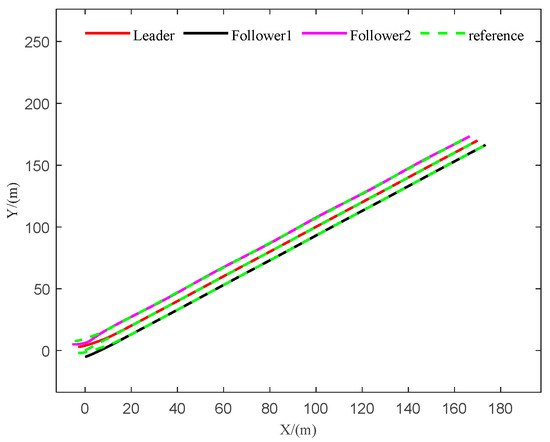
Figure 2. Formation with interference observers.

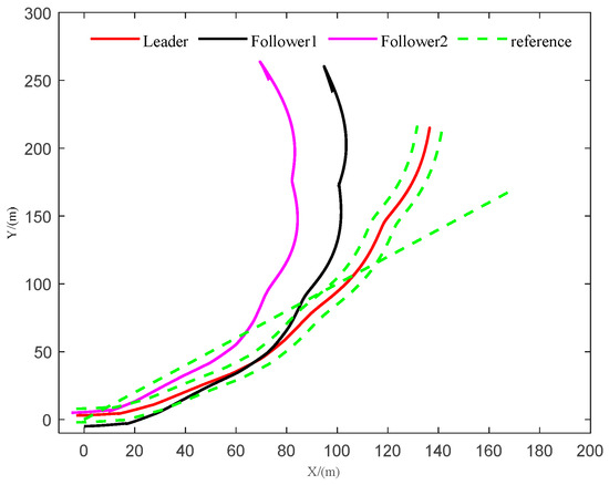
Figure 3. Formation without interference observers.

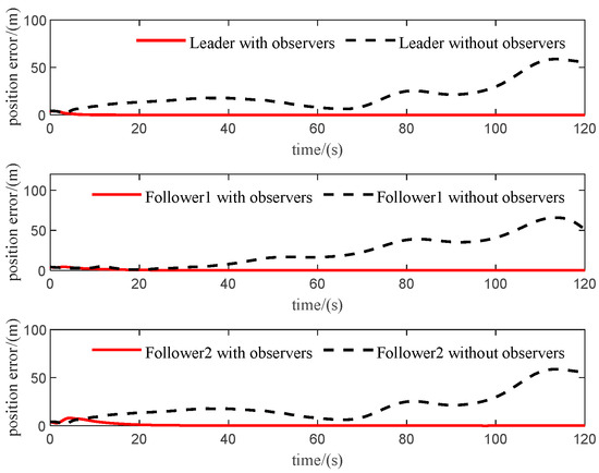
Figure 4. Comparison of positional errors.

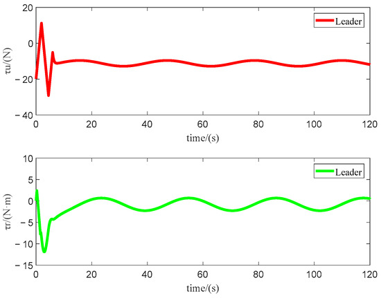
Figure 5. Changes shown by the leader AUV.

Figure 6. Changes shown by follower AUV 1.

Figure 7. Changes shown by follower AUV 2.

Figure 8. Velocities of the leader AUV.

Figure 9. Velocities of follower AUV 1.

Figure 10. Velocities of follower AUV 2.

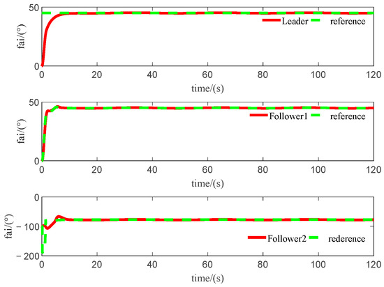
Figure 11. Heading angles of the AUVs.

Figure 12. Interference observation of the leader AUV.

Figure 13. Interference observation of follower AUV 1.

Figure 14. Interference observation of follower AUV 2.

The simulation results show that the formation trajectory-tracking error of the AUV essentially converged within 20 s, and there was no instability or divergence after convergence, which shows that the control algorithm is stable, reliable, and effective.

Figure 2, Figure 3, Figure 4, Figure 5, Figure 6, Figure 7, Figure 8, Figure 9, Figure 10, Figure 11, Figure 12, Figure 13 and Figure 14 show a straight-line trajectory with $u_d$ = 2 m/s, $r_d$ = 0, and a heading angle of π/4. These figures include the trajectory tracking, the position error, the force and torque change, the tracking of each state quantity, and the tracking of the interference observers for the leader AUV and for the follower AUVs.

5.2. Simulation Experiment 2 (Case 2): Circular Side-by-Side Queue

$u_d$ = 2 m/s and $r_d$ = 0.05° were selected to generate the trajectory of the leader AUV. The resulting trajectory was a circle. Table 4 shows the formation information.

Table 4. Formation information for the circular side-by-side queue.

Follower Boat Name	Distance L	Vehicle Direction Angle φ
Follower AUV 1	5 m	0°
Follower AUV 2	5 m	0°

The initial state of the leader autonomous underwater vehicle was state = [−3; 3; 0; 0.5; 0; 0; 0; 0]. The initial state of follower AUV 1 was gensui11 = [0; −5; 0; 0; 0; 0; 0; 0]. The initial state of follower AUV 2 was gensui12 = [−5; 5; 0; 0; 0; 0; 0; 0]. Table 5 shows the selection of controller parameters $k_1,k_2,k_3,k_4,k_5,k_6,k_7,{\lambda }_1,{\lambda }_2,{\lambda }_3$ for the leader AUV and follower AUVs 1 and 2.

Table 5. The control parameters of the formation (Case 2).

Leader AUV		Follower AUV 1		Follower AUV 2
$k_1$	0.5	$k_1$	0.1	$k_1$	0.31
$k_2$	8	$k_2$	60	$k_2$	62
$k_3$	0.7	$k_3$	1.02	$k_3$	0.5
$k_4$	0.0001	$k_4$	0.24	$k_4$	0.66
$k_5$	50	$k_5$	20	$k_5$	32
$k_6$	1.5	$k_6$	10	$k_6$	3
$k_7$	0.192	$k_7$	0.01	$k_7$	0.048
${\lambda }_1$	0.28	${\lambda }_1$	0.0001	${\lambda }_1$	0.001
${\lambda }_2$	1	${\lambda }_2$	12	${\lambda }_2$	0.001
${\lambda }_3$	1	${\lambda }_3$	18	${\lambda }_3$	0.1

These simulation results are shown in Figure 15, Figure 16, Figure 17, Figure 18, Figure 19, Figure 20, Figure 21, Figure 22, Figure 23, Figure 24, Figure 25, Figure 26 and Figure 27.

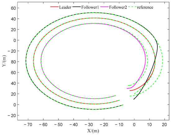
Figure 15. Formation with interference observers.

Figure 16. Formation without interference observers.

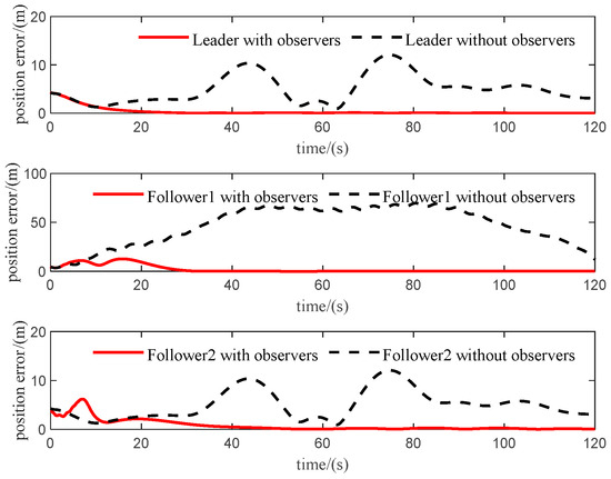
Figure 17. Comparison of positional errors.

Figure 18. Changes shown by the leader AUV.

Figure 19. Changes shown by follower AUV 1.

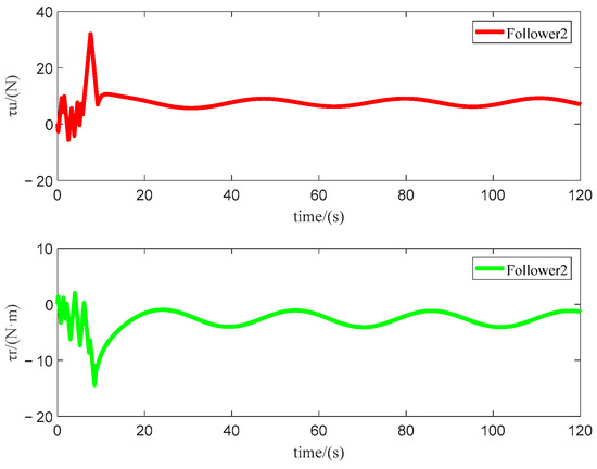
Figure 20. Changes shown by follower AUV 2.

Figure 21. Velocities of the leader AUV.

Figure 22. Velocities of follower AUV 1.

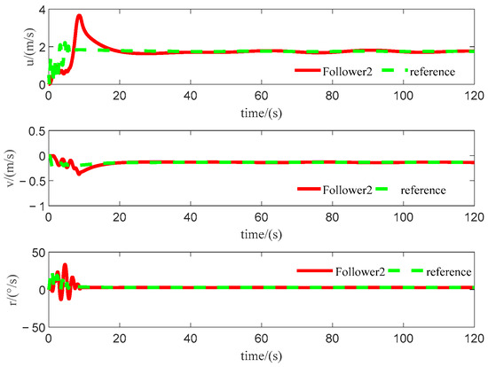
Figure 23. Velocities of follower AUV 2.

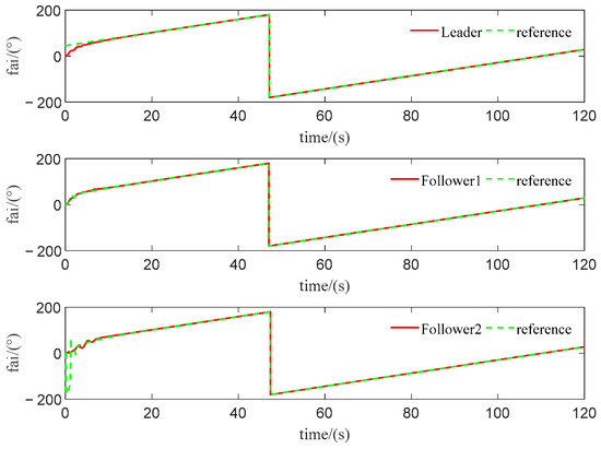
Figure 24. Heading angles of the AUVs.

Figure 25. Interference observation of the leader AUV.

Figure 26. Interference observation of follower AUV 1.

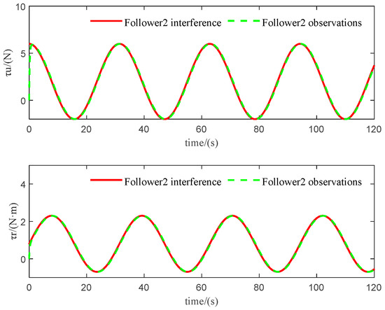
Figure 27. Interference observation of follower AUV 2.

Figure 15, Figure 16, Figure 17, Figure 18, Figure 19, Figure 20, Figure 21, Figure 22, Figure 23, Figure 24, Figure 25, Figure 26 and Figure 27 show a circular trajectory with $u_d$= 2 m/s, $r_d$ = 0.05, and a heading angle of π/4. These figures include the trajectory tracking, the position error, the force and torque change, the tracking of each state quantity, and the tracking of the interference observers for the leader AUV and the follower AUVs.

In both cases, we compared the trajectory tracking and position errors of the interference with and without the disturbance observer, and it was observed that the formation could maintain the stability of trajectory tracking and the rapid convergence of the position error under both working conditions after adding the interference observer. It can be seen from the data in the figures that the AUVs’ formation was able to reach the target formation in a very short time, while the oscillation time was short, the error was small, and the error quickly converged to zero. And the AUVs could still maintain a stable formation under the action of interference.

In summary, these simulation experiments verify that the control method based on the backstepping method and cascade system is effective, and the trajectory error and position error caused by interference can be effectively offset after the interference observer is added.

6. Conclusions and Discussion

Based on a control method using a cascading system and the Lyapunov direct method, the formation trajectory-tracking problems of underactuated AUVs were combined in this study. Different from the traditional full-trajectory guidance, which uses the expected trajectory of the leader AUV for formation control, this paper adopts the actual trajectory of the leader AUV for formation control, which can make the formation situation closer to the actual situation. By using global differential homeomorphism transformation, the complex formation control system is decomposed into a cascaded system that is easy to analyze. Based on the actual trajectory of the leader AUV, the AUV formation is determined. The formation control rate was designed by using the direct backstepping method and Lyapunov theory. In addition, an interference observer was added to ensure that the trajectory error can be reduced quickly. Finally, the stability and effectiveness of this method were verified using simulation experiments. Considering the actual situation, in the simulation of the two working conditions, interference was added to the force and torque in the form of a combination of constant and sinusoidal signals [29] to verify the robustness of the control algorithm. To maintain the expected formation, the change in longitudinal force and torque was consistent with the interference change form. Compared with the complexity of the actual sea state, the interference added in this paper is in the form of a common sinusoidal function; at the same time, only the straight-line side-by-side queue and the circular side-by-side queue are considered, which is not enough to represent the variety of working conditions.

Future research will focus on the following two aspects:

(1) Previous studies are mostly based on theory, and the process of sea trials is rarely recorded in the various studies in the literature. However, in actual tasks, the marine environment is complicated and changeable, the accuracy of ranging and direction-finding sensors is usually low, and the underwater acoustic communication may experience errors or even be interrupted, which can make the conventional formation control algorithm ineffective. For the study of AUV formation, the ultimate goal should be to realize its practicability, which is the only way to achieve formation control.

(2) Under the premise of practicality, the AUV formation structure must be heterogeneous, so that the formation system can complete more complex tasks. However, most of the existing studies in the literature remain focused on the analysis of isomorphic systems, and there are still gaps in the research regarding the formation control of heterogeneous systems. It is thus necessary to design a formation control algorithm for heterogeneous AUV cluster systems.

References

- Zwolak, K.; Wigley, R.; Bohan, A.; Zarayskaya, Y.; Bazhenova, E.; Dorshow, W.; Sumiyoshi, M.; Sattiabaruth, S.; Roperez, J.; Proctor, A.; et al. The Autonomous Underwater Vehicle Integrated with the Unmanned Surface Vessel Mapping the Southern Ionian Sea the Winning Technology Solution of the Shell Ocean Discovery XPRIZE. Remote Sensing. 2020, 12, 1344. [Google Scholar] [CrossRef]
- Tan, K.-H.; Lewis, M. Virtual structures for high-precision cooperative mobile robotic control. In Proceedings of the IEEE/RSJ International Conference on Intelligent Robots and Systems, IROS ’96, Osaka, Japan, 8 November 1996; Volume 1, pp. 132–139. [Google Scholar] [CrossRef]
- Wilson, S.; Pavlic, T.P.; Kumar, G.P.; Buffin, A.; Pratt, S.C.; Berman, S. Design of ant-inspired stochastic control policies for collective transport by robotic swarms. Swarm Intell. 2014, 8, 303–327. [Google Scholar] [CrossRef]
- Doctor, S.; Venayagamoorthy, G.K.; Gudise, V.G. Optimal PSO for collective robotic search applications. In Proceedings of the 2004 Congress on Evolutionary Computation. (IEEE Cat. No. 04TH8753), Portland, OR, USA, 19–23 June 2004; IEEE: Piscataway, NJ, USA, 2004; Volume 2. [Google Scholar]
- Ren, W.; Sorensen, N. Distributed coordination architecture for multi-robot formation control. Robot. Auton. Syst. 2008, 56, 324–333. [Google Scholar] [CrossRef]
- Wang, J.; Wang, C.; Wei, Y.; Zhang, C. Observer-Based Neural Formation Control of Leader–Follower AUVs with Input Saturation. IEEE Syst. J. 2020, 15, 2553–2561. [Google Scholar] [CrossRef]
- Askari, A.; Mortazavi, M.; Talebi, H.A. UAV formation control via the virtual structure approach. J. Aerosp. Eng. 2015, 28, 04014047. [Google Scholar] [CrossRef]
- Ge, S.; Fua, C.-H. Queues and artificial potential trenches for multirobot formations. IEEE Trans. Robot. 2005, 21, 646–656. [Google Scholar] [CrossRef]
- Fua, C.-H.; Ge, S.S.; Do, K.D.; Lim, K.W. Multi-Robot Formations based on the Queue-Formation Scheme with Limited Communications. In Proceedings of the 2007 IEEE International Conference on Robotics and Automation IEEE, Rome, Italy, 10–14 April 2007. [Google Scholar]
- Balch, T.; Arkin, R. Behavior-based formation control for multirobot teams. IEEE Trans. Robot. Autom. 1998, 14, 926–939. [Google Scholar] [CrossRef]
- Panagou, D.; Kumar, V. Cooperative Visibility Maintenance for Leader–Follower Formations in Obstacle Environments. IEEE Trans. Robot. 2014, 30, 831–844. [Google Scholar] [CrossRef]
- Kumar, R.; Stover, J.A. A behavior-based architecture for intelligent controller design. In Proceedings of the 37th IEEE Conference on Decision and Control (Cat. No.98CH36171), Tampa, FL, USA, 18 December 1998; IEEE: Piscataway, NJ, USA, 1998. [Google Scholar]
- Ji, M.; Ferrari-Trecate, G.; Egerstedt, M.; Buffa, A. Containment Control in Mobile Networks. IEEE Trans. Autom. Control 2008, 53, 1972–1975. [Google Scholar] [CrossRef]
- Li, X.; Zhu, D. An Adaptive SOM Neural Network Method to Distributed Formation Control of a Group of AUVs. IEEE Trans. Ind. Electron. 2018, 65, 8260–8270. [Google Scholar] [CrossRef]
- Ding, G.; Zhu, D.; Sun, B. Formation control and obstacle avoidance of multi-AUV for 3-D underwater environment. In Proceedings of the 2014 33rd Chinese Control Conference (CCC) IEEE, Nanjing, China, 28–30 July 2014. [Google Scholar]
- Kartal, Y.; Subbarao, K.; Gans, N.; Dogan, L.; Lewis, F. Distributed backstepping based control of multiple UAV formation flight subject to time delays. IET Control Theory Appl. 2020, 14, 1628–1638. [Google Scholar] [CrossRef]
- Dong, Z.; Liu, Y.; Wang, H.; Qin, T. Method of cooperative formation control for underactuated USVs based on nonlinear backstepping and cascade system theory. Pol. Marit. Res. 2021, 28, 149–162. [Google Scholar] [CrossRef]
- Dong, Z.; Qi, S.; Yu, M.; Zhang, Z.; Zhang, H.; Li, J.; Liu, Y. An improved dynamic surface sliding mode method for autonomous cooperative formation control of underactuated USVs with complex marine environment disturbances. Pol. Marit. Res. 2022, 29, 47–60. [Google Scholar] [CrossRef]
- Gu, N.; Wang, D.; Peng, Z.; Li, T.; Tong, S. Model-free containment control of underactuated surface vessels under switching topologies based on guiding vector fields and data-driven neural predictors. IEEE Trans. Cybern. 2021, 52, 10843–10854. [Google Scholar] [CrossRef] [PubMed]
- Zhang, X.; Zhang, Q.; Ren, H.X.; Yang, G.P. Linear reduction of backstepping algorithm based on nonlinear decoration for ship course-keeping control system. Ocean Eng. 2018, 147, 1–8. [Google Scholar] [CrossRef]
- Fu, M.; Wang, D.; Wang, C. Formation control for water-jet USV based on bio-inspired method. Ocean Eng. 2018, 32, 117–122. [Google Scholar] [CrossRef]
- Qin, H.; Li, C.; Sun, Y.; Deng, Z.; Liu, Y. Trajectory tracking control of unmanned surface vessels with input saturation and full-state constraints. Int. J. Adv. Robot. Syst. 2018, 15, 1729881418808113. [Google Scholar] [CrossRef]
- Wang, J.; Wang, C.; Wei, Y.; Zhang, C. Filter-backstepping based neural adaptive formation control of leader-following multiple AUVs in three dimensional space. Ocean Eng. 2020, 201, 107150. [Google Scholar] [CrossRef]
- Wang, F.; Gao, Y.; Zhou, C.; Zong, Q. Disturbance observer-based backstepping formation control of multiple quadrotors with asymmetric output error constraints. Appl. Math. Comput. 2022, 415, 126693. [Google Scholar] [CrossRef]
- Yan, Z.; Liu, Y.; Zhou, J.; Zhang, G. Moving Target Following Control of Multi-AUVs Formation Based on Rigid Virtual Leader-Follower Under Ocean Current. In Proceedings of the IEEE 34th Chinese Control Conference (CCC) IEEE, Hangzhou, China, 28–30 July 2015. [Google Scholar]
- Wan, L.; Dong, Z.; Li, Y.; Liu, T.; Zhang, G. Trajectory tracking control of non-completely symmetric underactuated high-speed unmanned marine vehicle. J. Electr. Eng. Control 2014, 18, 95–103. [Google Scholar]
- Fossen, T.I. Handbook of Marine Craft Hydrodynamics and Motion Control; John Wiley & Sons: Hoboken, NJ, USA, 2011. [Google Scholar]
- Ghommam, J.; Mnif, F.; Benali, A.; Derbel, N. Asymptotic backstep** stabilization of an underactuated surface vessel. IEEE Trans. Control Syst. Technol. 2006, 14, 1150–1157. [Google Scholar] [CrossRef]
- Gao, Z.; Guo, G. Adaptive formation control of autonomous underwater vehicles with model uncertainties. Int. J. Adapt. Control Signal Process. 2018, 32, 1067–1080. [Google Scholar] [CrossRef]
Disclaimer/Publisher’s Note: The statements, opinions and data contained in all publications are solely those of the individual author(s) and contributor(s) and not of MDPI and/or the editor(s). MDPI and/or the editor(s) disclaim responsibility for any injury to people or property resulting from any ideas, methods, instructions or products referred to in the content. |
© 2024 by the authors. Licensee MDPI, Basel, Switzerland. This article is an open access article distributed under the terms and conditions of the Creative Commons Attribution (CC BY) license (https://creativecommons.org/licenses/by/4.0/).