Abstract
The efficiency of collecting and distributing goods has been improved by establishing railway lines that serve new automated container terminals (ACTs) and by constructing central railway stations close to ports. To aid in this process, intelligent guided vehicles (IGVs), which are renowned for their flexibility and for the convenience with which one can adjust their number and speed, have been developed to be used as horizontal transport vehicles that can transport goods between the railway yard and the front of the port. However, they also introduce some difficulties and complexities that affect terminal scheduling. Therefore, we took the automated rail-mounted container gantry crane (ARMG) scheduling problem as our main research object in this study. We established a mixed-integer linear programming (MILP) model to minimize the makespan of ARMGs, designed an adaptive large neighborhood search (ALNS) algorithm, and explored the influence of IGV configuration on ARMG scheduling through a series of experiments applied to a series of large-scale numerical examples. The experimental results show that increasing the number of IGVs can improve the operational efficiency of railway yards, but this strategy reduces the overall time taken for the ARMG to complete various tasks. Increasing or decreasing the speed of the IGVs within a given range has a clear effect on the problem at hand, while increasing the IGV travel speed can effectively reduce the time required for the ARMG to complete various tasks. Operators must properly adjust the IGV speed to meet the requirements of the planned operation.
1. Introduction
As sea–rail intermodal container transportation has developed, an increasing amount of attention has been paid to improving the efficiency of the connection between water transportation modes and railways. In some newly built ACTs, the long-standing physical barrier that has existed between ACTs and central container railway stations has begun to break down, and some of these ACTs have been amalgamated into the same customs supervision areas and operational areas to achieve integrated operations across regions; one such example is the Qinzhou ACT in China. As the time taken to process transfers of goods between railways and ports has decreased, the transportation of goods between railways and port terminals has become easier. Mobile machinery is responsible for the improved connection between railways and port terminals, and it is through this connection that containers are transferred between the railway yards and the front areas of ACTs. Studying the configuration of mobile machinery is of great significance to improve logistics, cost control, and the discharge of pollution in sea–rail intermodal transport.
The mobile machinery used in a typical ACT includes AGVs and IGVs. The “Magnetic rail + AGV” is the “standard configuration” for most ACTs. AGVs are required to bury tens of thousands of magnetic rails in the ground to facilitate automatic driving. However, this is a long process, and laying the magnetic rails incurs high costs. Compared with AGVs, IGVs are more flexible and can operate without the need for any markers. There is no need to make complex changes to the original layout of the railway yard as an IGV can travel without magnetic rails, making their paths flexible and changeable, and allowing them to freely travel around terminals. As IGV routes are flexible and changeable, their schedules can be adjusted according to actual production needs, and the accuracy of their positioning can reach ±1 mm. As autonomous driving and 5G communication technologies continue to develop, the broad prospects of the application of IGVs in the construction of new ACTs and the transformation of traditional container terminals become more apparent [1]. In recent years, IGVs have been introduced at the Yongzhou Terminal of Ningbo Zhoushan Port, the Nansha Phase IV Terminal of Guangzhou Port, and the Qinzhou ACT of Beibuwan Port. AGVs and IGVs are the main types of mobile machinery used to transport containers between the railway yards and front areas of automated container terminals (RYACTs), and this study takes Beibuwan Port’s Qinzhou ACT as an example. As the main horizontal transportation machinery used at the Qinzhou ACT, we chose IGVs as the object of our study and we investigated the influence of IGV configuration on equipment scheduling in the railway yards of automated container terminals. Importantly, research on IGV configurations has practical significance for controlling costs and preventing collisions in the railway yards of ACTs.
In this study, the Qinzhou ACT of Beibuwan Port was taken as a reference, and the coordinated scheduling of ARMGs and IGVs was taken as the main research object. To solve the problem, a MILP model was established, and a random search algorithm (RSA) and ALNS algorithm were designed. Through a series of experiments, the influence of the IGV configuration on ARMG scheduling in central railway depots was explored. The contributions of this paper are as follows: (1) A MILP model was established to solve the problem of coordinating the schedules of ARMGs and IGVs in the RYACTs. (2) An ALNS algorithm was similarly designed to solve this problem. (3) The influence of both the number of IGVs and their speed on ARMG scheduling was also discussed.
2. Literature Review
Several researchers have conducted studies on the mechanical scheduling of berths, storage yards, and RYACTs. Quay cranes (QCs) are positioned at the forefront of ACTs, and the equipment in railway yards generally includes yard cranes (YCs), ARMGs, and double-cantilever rail cranes or rail-mounted gantry cranes. The horizontal transportation vehicles include automated guided vehicles (AGVs), autonomous straddle carriers (ASDCs), and intelligent guided vehicles (IGVs).
Some scholars have studied single-machine scheduling problems from the perspectives of the order of operations, the allocation of storage space within the yard, and energy consumption. Chu et al. [2] studied multi-crane scheduling problems in adjacent container blocks. In a previous study, Luo et al. [3] focused on AGV scheduling and container storage problems. Xiang and Liu [4] built a nested semi-open queueing network model to consider AGV battery management. Cao et al. [5] studied AGV scheduling and bidirectional conflict-free path problems. Considering that the battery-powered AGV scheduling problem is time-intensive, Yang et al. [6] proposed a partitioning method based on depth-first and breadth-first searches to resolve the model. Oladugba et al. [7] designed an algorithm based on the modified Johnson algorithm to resolve the twin-ASC scheduling problem. Gao et al. [8] proposed a digital twin-based approach to optimize the operation of ASCs in terms of energy consumption.
The problem of the joint scheduling of vehicles in the wharf front, yard, and railway yard is also an important branch of mechanical scheduling research. Many authors have carried out research on the problem of the joint scheduling of ship loading/unloading and horizontal transportation [9,10,11,12,13]. Skaf, Lamrous, Hammoudan, and Manier [11] designed a heuristic algorithm and obtained superior results compared to the real results from a port in Tripoli. Liu, Zhu, Wang, and Wang [13] established a bi-level programming model to determine the paths of AGVs and obtain the YC scheduling scheme. Several authors have studied the problem of the joint scheduling of horizontal transportation and yard storage [14,15,16]. Wang, Hu, and Tian [15] studied the problem of scheduling both AGVs and ASCs by considering hybrid, buffer, and direct modes of transporting containers. Zhang, Li, and Sheu [16] researched the problem of the integrated scheduling of AGVs and double YCs in a one-yard block. Numerous authors have studied the problem of the joint scheduling of ship loading/unloading, horizontal transport, and yard storage [17,18,19,20,21,22,23,24,25,26,27]. Luo and Wu [22] established a model to ensure a minimum berthing time. Xu et al. [24] focused on conflict-free AGVs, dual-trolley QCs, and dual-cantilever rail cranes, proposing an integrated scheduling optimization model characterized by a U-shaped layout. Niu et al. [25] studied the problem of scheduling automated DCRCs, QCs, IGVs, and external trucks, aiming to reduce energy consumption. The problem of integrated scheduling for YCs, QCs, and AGVs has also been studied. Taking the ACT layout data of Yangshan Port as an example, Yue, Fan, and Fan [26] studied block allocation and scheduling. To solve the “QC-ASDC-ARMG” complex scheduling problem, Yu et al. [27] designed a particle swarm optimization algorithm based on adaptive tent chaos mapping. In order to reflect the complex interactions between pieces of terminal equipment such as rail gantry cranes (RGCs), IGVs, and double-cantilever rail cranes, Li, Yan, and Xu [28] included safe-distance and non-crossing constraints. To optimize the joint scheduling of ARMGs and external truck arrangements, He et al. [29] designed a study with multiple objectives, including balancing these arrangements across periods of time and among different blocks. To design a new concept based on multi-story frame bridges, Zhen et al. [30] studied how to schedule QCs and bridge cranes that transfer containers between different stories.
In summary, many researchers have studied the mechanical scheduling of key steps in the container transportation process such as ship loading/unloading and container stacking in ACTs from different perspectives, but few studies have been conducted on the combination of mobile machinery configurations and railway yard operations. Yang et al. [31] studied the joint scheduling of ARMGs and AGVs alongside the trains, yard, and ships to minimize the energy consumption within the port, and then obtained a reasonable ratio between ARMGs and AGVs. Yang et al. [32] proposed a strategy to adjust the number of AGVs to accommodate delays in ship arrivals and changes in the types of train containers, but did not discuss the effect of AGV speed on scheduling. Chen and Liu [33] studied the “RYACT–train” cooperative optimization problem. On the basis of this previous research, this paper takes the U-shaped layout at the Qinzhou ACT as a reference, the “IGV-RYACT–train” scheduling problem as the main research object, establishes a MILP model, and discusses the influence of IGV configuration on ARMG scheduling through a series of experiments.
3. Description of the Scheduling Problem
Traditional ACTs with a vertical block layout have ARMGs at both ends (the “land side” and “sea side”), so their civil engineering and equipment requirements are higher. However, the wharf in the Qinzhou Port area is long and deep, making it unsuitable for traditional technology; as such, Qinzhou Port adopted a “U-shaped” layout.
The “U-shaped” layout (Figure 1) facilitates traffic diversion; that is, through the vertical layout of the storage yard and the alternating “U”- and “I”-type roads, the traffic diversion, physical isolation, and mutual non-interference between the external trucks and the IGVs can enable the same storage yard to implement both land-side and sea-side collection and distribution operations, while ensuring the safety of these automated operations.
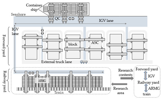
Figure 1.
The automated container terminal area covered by the research.
This paper explores the ARMG–IGV coordinated scheduling problem in an RYACT. ARMGs and IGVs are the main pieces of equipment used for the loading, unloading, and transporting of containers between trains, the RYACT, and the front area of the port. By using the arrival time of the train and the container handling information, the ARMG configured in the RYACT can operate between the inbound trains and the IGVs simultaneously. The ARMG’s operating processes include loading/unloading the trains and IGVs.
The IGV’s docking position within the IGV lane corresponds to the bay in which the container is stored in the RYACT, the main purpose of which is to decrease the movement time of the ARMG and enhance its efficiency. The ARMG’s working points include the location of the train carriage, the position of the container stored in the block, and the IGV docking position. The ARMG does not need to move within this bay when it is handling a container transported by an IGV.
4. Problem Formulation
In this section, a MILP model is formulated to minimize the makespan of ARMGs.
4.1. Assumptions
According to the above descriptions, the assumptions made in this study can be summarized as follows:
- (1)
- Repositioning or rehandling activities that are included in the ARMG’s operations are not taken into consideration;
- (2)
- Unloading containers from the train does not affect the subsequent loading operation;
- (3)
- The speed of the ARMGs is fixed;
- (4)
- The origin–destination (OD) locations of the containers handled by the ARMGs are known;
- (5)
- The time taken for the ARMG to grab a container is equal to the time it takes for it to release it;
- (6)
- To ensure operational safety, the trolley within an ARMG remains stationary while its gantry moves;
- (7)
- Congestion and IGV breakdowns are not considered.
4.2. Parameters and Decision Variables
The indices, parameters, and variables used in the proposed model are summarized in Table 1, Table 2 and Table 3, respectively.

Table 1.
Indices used in the formulation of the model.
Table 2.
Parameters used in the formulation of the model.
Table 3.
Decision variables used in the formulation of the model.
4.3. Model Formulation
This study investigated the problem of coordinating the schedules of ARMGs and IGVs, such that an ARMG can load/unload IGVs and trains simultaneously, aiming to improve the production efficiency of ARMGs. The time taken for an ARMG to complete the whole set of tasks should be as short as possible, so the goal of the model is to minimize the makespan of ARMGs. The total task completing time should be calculated according to the ARMG with the longest operation time. Therefore, Formula (1) was used as the objective function, and the model was constructed as follows:
subject to:
Constraint (2) can li mit the starting time of the initial task handled by the ARMG, where . Constraints (3) and (4) convey that the ARMG’s activity starts with a virtual start task and terminates with a virtual end task. Constraint (5) can keep the flow of task balanced. When an ARMG is continuously performing tasks and , Constraint (6) is used to ensure a minimum interval between the ARMG’s completion of task and the beginning of task . Constraint (7) describes the connection between the ARMG beginning and completing task . Constraints on the IGV transport containers include the following: Constraint (8) ensures that the completion of an ARMG task occurs at the beginning of an IGV transport task. Constraints (9) and (10) are used to determine the number of IGVs used in a joint scheduling problem. Constraint (11) is used to ensure tasks flow balancing for IGVs. When an IGV is continuously performing transport tasks and , Constraint (12) is used to ensure a minimum interval between the IGV’s completion of task and the beginning of task . Constraint (13) describes the connection between the IGV beginning and completing transport task . Constraint (14) represents the sequence in which any two tasks, i and j, should be finished by an ARMG. The intermediate nodes within the time taken to complete each task are calculated according to the types of tasks being carried out by the ARMG. Constraints (15)–(17) are used to avoid interference between adjacent ARMGs. Constraints (18) and (19) control the range of variable values.
5. Proposed Algorithm
The ARMG scheduling stage in the ARMG and IGV scheduling problem can be viewed as several traveling salesman problems, and the interference among the different operational cranes should be considered at the same time. The studied problem is NP-hard, and it is difficult to find exact solutions and for optimization solvers such as CPLEX to solve mid- and large-scale examples of this problem in an acceptable amount of time. Many different heuristic algorithms have been used to solve scheduling optimization problems in ACTs with mid- or large-scale examples, including a spatiotemporally greedy genetic algorithm [13], the cuckoo search algorithm [34], and a reinforcement learning-based hyper-heuristic genetic algorithm [24]. Heuristics based on large neighborhood search (LNS) have presented notable success in the fields of scheduling and transportation [35]. Ropke and Pisinger [36] adjusted LNS by defining several destroy-and-repair methods, and they named their algorithm ALNS. ALNS can adaptively select the destroy–repair operators within each iteration, and has been used to solve various routing problems [37,38,39,40,41,42,43], such as transportation planning and heterogeneous container loading problems. Considering the remarkable success of ALNS, we decided to apply the ALNS algorithm to our problem.
5.1. Encoding and Decoding Methods
The ARMG task sequence, that is, the order of the coding, is used to represent the relative order of the tasks handled by ARMGs, where the coded value represents the task’s sequence number and its position represents the task assignment. The ARMG task sub-sequence generation procedures are shown in Figure 2 according to a specific ARMG task sequence. Considering the ARMG task assignment, task types, and the operation mode of loading/unloading synchronization, the ARMG task sub-sequence for each ARMG can be generated. The AMRG’s task sub-sequence corresponding to the encoding sequence (i.e., the ARMG’s task sequence) is generated from the input. Finally, the decoding method for evaluating the ARMG task sequence can be designed according to the ARMG task sub-sequence that has been generated. In this process, the priority of all tasks handled by multiple ARMGs is determined by the ARMG task sequence to avoid any interference between adjacent ARMGs.
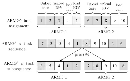
Figure 2.
ARMG task sub-sequence generation procedure.
In the process of loading/unloading a train, the positions of ARMGs at the beginning of a task are not consistent with those at the end. At this time, each task performed by the ARMG has some key time nodes: the starting time ( and the completing time (). During the loading or unloading of an IGV by an ARMG, the ARMG stays within its bay. However, to fully describe the process of an ARMG carrying out a task between the block and the IGV, the two critical time nodes, the starting time () and the completing time (), need to be recorded. The earliest starting and completing times for the ARMG task, and the earliest starting and completing times for the IGV transportation task, can be calculated according to the descriptions of the problem and the model [M1]. Detailed steps of the proposed decoding method are shown in Table 4.
Table 4.
Decoding steps.
5.2. Random Search Algorithm
To verify the feasibility of encoding and decoding, and to search the solution space quickly, we used an RSA to optimize the joint scheduling of ARMGs and IGVs in the RYACT. The process of designing the RSA was similar to that described in our previous paper [33]. Therefore, IGV job sequence scoring was added. Finally, the problem’s target value and the ARMG and IGV operation time nodes were returned. The specific steps in the RSA are presented in Table 5.
Table 5.
RSA steps.
5.3. Adaptive Large Neighborhood Search
In this section, ALNS is applied to optimize the job sequence for the given initial coding sequence. The neighborhood search operator is set to search the neighborhood adaptively to generate a new ARMG task sequence. The ARMG task sequence is optimized iteratively, and the objective values and the schedules of the ARMGs and IGVs are returned.
- (1)
- Encoding and decoding method:
The encoding and decoding methods of the ALNS are set according to Section 5.1. The order coding shown in Figure 2 is used as the encoding method, and the decoding method is shown in Table 4.
- (2)
- Generating an initial solution:
An initial solution for this algorithm can be generated by the RSA with a given iteration number.
- (3)
- The pairs of destroy–repair operators for generating the neighborhood:
Operators include single-point reinsertion, fragment reinsertion, local reverse order, two-point exchange, fore-and-aft interchange, and regeneration [33].
- (4)
- The stopping criteria:
The algorithm will stop when the iteration number of the algorithm reaches the maximum number of iterations () or when the number of iterations in which the optimal value remains unchanged reaches the maximum number of stall score iterations () [33].
- (5)
- The algorithm’s steps:
The steps involved in ALNS are exhibited in Table 6.
Table 6.
The steps involved in ALNS.
6. Computational Experiments
The experimental dataset was composed of randomly selected data from the original dataset of wharf operation tasks. The input parameters of the ARMGs and IGVs are listed in Table 7, and the ALNS settings are presented in Table 8. The algorithm was implemented in MATLAB R2017b, and all the solution procedures were performed on a computer with an a computer with an Intel(R) Core(TM) i5-7200U CPU @ 2.50 GHz (Intel, Santa Clara, CA, USA), 8 GB RAM, and the Windows 10 operating system.
Table 7.
The ALNS settings [31].
Table 8.
The input parameters [31] for ARMGs and IGVs.
6.1. Comparison of Computing Performance of [M1], RSA, and ALNS
The experimental steps can be summarized as follows: (1) Set the number of tasks as 10, 12, …, 30, 40, …, 160 and create examples according to the experimental dataset. (2) Set the number of RSA iterations to . (3) Set the ALNS parameters as shown in Table 7, and set other parameters as shown in Table 8. (4) For each set of tasks, solve the model [M1] via the solver CPLEX and obtain the optimal solution, and then run the RSA and ALNS to return the results. The experimental results are presented in Table 9.
Table 9.
Computing performance of [M1], RSA, and ALNS (the units for , , and are seconds).
As shown in Table 9, model [M1] has an outstanding computational performance in cases with a small number of tasks. For instance, it can obtain results quickly in a limited time when there are no more than 26 tasks. When the number of tasks ranges from 28 to 30, only feasible solutions can be obtained by the model. Appendix A shows the computational times and objective values corresponding to 15 different cases of different small sizes solved by the model [M1]. It can be seen in Appendix A that as the number of tasks increases, the model [M1] cannot obtain the optimal solution to the problem in a limited time, and the range of objective values is small. Secondly, the RSA can quickly solve cases of various sizes, but its optimization is poor. Appendix B shows a comparison of the solution results when the number of iterations increases. Let us set the number of RSA iterations to and the number of ALNS iterations to ; as can be seen in Appendix B, when the number of iterations is increased, the optimal value determined by the RSA is still smaller than the optimal value determined by ALNS. Finally, ALNS can resolve cases of various sizes within 9 s, has a good optimality in solving small- and medium-scale examples (no more than 3.8% compared with [M1]), and has a good convergence for multiple solutions.
Other algorithms are often used to solve scheduling optimization problems in ACTs. Appendix C shows the use of a genetic algorithm as an example to compare computing performance with ALNS. In this group of examples, the ALNS algorithm demonstrates a better performance. In future work, ALNS will be applied to solve the problem of the influence of the IGV configuration on equipment scheduling in the RYACT.
6.2. The Effect of the Number of IGVs on the Target Value
The experimental steps can be summarized as follows: (1) Set the number of tasks to 60, 80, …, 140; the corresponding ARMG number is 5. (2) For each combination of task and ARMG number, set the IGV number to 2, 3, …, 8. (3) For each example, run the ALNS algorithm to solve the example 10 times and return the minimum value. The experimental results are exhibited in Figure 3.
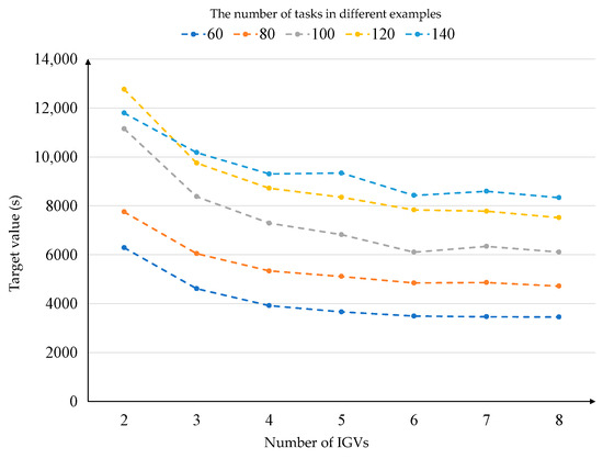
Figure 3.
The effect of the number of IGVs on target values.
As shown in Figure 3, for each example, with an increase in the number of IGVs, the target value first decreases and then tends to converge. According to the experimental results, when the number of IGVs is six, the method can be adapted to most cases. ACT managers can use this method to configure the appropriate number of IGVs, as implementing more IGVs is not always the optimal solution.
6.3. The Effect of IGV Speed on the Target Value
The experimental steps can be summarized as follows: (1) Set the number of tasks to 60, 80, …, 140; the corresponding number of ARMGs is five, and the corresponding number of IGVs is five. (2) Based on the initial IGV speed, set the new IGV speed according to the difference [−50%, −25%, 0, +25%, +50%], and then construct a new calculation. (3) For each example with different numbers of tasks, run ALNS to solve the example 10 times and return the minimum value. The experimental results are exhibited in Figure 4.
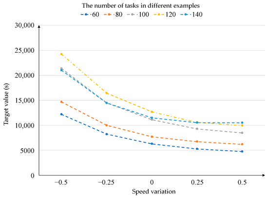
Figure 4.
The effect of IGV speed on target values.
According to Figure 4, changing the IGV’s travel speed clearly influences the time taken for the ARMG to complete a series of tasks. Transportation safety, energy consumption, engine power, container’s weight, and other factors can restrict the IGV speed in a container terminal. Considering the safety of the traffic, the speed of IGVs can be adjusted flexibly within the range of 25% in actual operation. From the experimental data, it can be seen that when the speed is increased by 25%, the time taken to complete the tasks is shortened by 14% on average, and when the speed is reduced by 25%, the time taken to complete the tasks is increased by 30% on average. Therefore, increasing the IGV travel speed can effectively reduce the task completion time, while conversely, reducing the IGV travel speed leads to a sharp rise in the task completion time. To take the operation efficiency and energy consumption of the ACT into account, operators must properly adjust the IGV speed to meet the requirements of the expected operation plan. Moreover, to reduce the impact on the operation of the central railway station, the IGVs at the front of the port must actively move out of the way when they intersect with an IGV from the RYACT.
7. Conclusions
This study explored the influence of IGV configurations, numbers, and speed adjustments on ARMG scheduling problems in the RYACT, in which the sequence of ARMGs, and the assignment and sequence of IGVs are fixed. Aiming to minimize the makespan of ARMGs, a MILP model was established, and an ALNS algorithm was designed. Through a series of experiments, the influence of the IGV configuration on ARMG scheduling was discussed in the case of different scales. The experiment revealed that increasing the number of IGVs can improve the efficiency of the railway yard, but the influence of increasing the number to a certain value on the overall task completion time of ARMGs is reduced, and the appropriate number of IGVs should be configured during task scheduling. In the experimental example in this paper, six IGVs were found to be most suitable for completing the tasks. From the experimental data, when the speed is increased by 25%, the time taken to complete a task is shortened by 14% on average, and when the speed is reduced by 25%, the time taken to complete a task is increased by 30% on average. Therefore, speed has a clear influence on task completion, whereby increasing the IGV travel speed can effectively reduce the time it takes ARMGs to complete tasks, while conversely, reducing the IGV travel speed leads to a sharp rise in the task completion time. To reduce the impact on the operation of the central railway station, an IGV from the front yard must actively yield when it intersects with an IGV from the RYACT. This study can help to provide a reference for resource conservation and avoiding collisions at ports. More practical constraints will be considered in future studies, such as constraints on train arrival time windows, restrictions on the number of machines, and environmental requirements. Although the proposed model and algorithm provide a good method and suggestions for IGV configuration, the algorithm designed for handling more loading and unloading tasks still needs to be improved, and the method for optimizing scheduling, considering more freight tasks and faster trains entering and leaving the railway yard, still needs to be studied. ACT managers also need to consider the energy consumption of IGVs, the configuration of other machinery, and the overall efficiency of the port area, all of which are worthy of further study.
Author Contributions
Original draft, modelling, algorithm design, formal analysis, and writing the paper, H.C.; verification, corrections, experiment supervision, and reviewing the paper, W.L. All authors have read and agreed to the published version of the manuscript.
Funding
This work was supported by the Fujian Provincial Department of Education’s Young and Middle-Aged Teachers Education Research Project (Grant No. JAT220190).
Institutional Review Board Statement
Not applicable.
Informed Consent Statement
Not applicable.
Data Availability Statement
Data are contained within the article.
Conflicts of Interest
The authors declare no conflicts of interest.
Abbreviations
The following abbreviations are used in this manuscript:
| Abbreviation | Full Name |
|---|---|
| ACT | automated container terminal |
| IGV | intelligent guided vehicle |
| ARMG | automated rail-mounted container gantry crane |
| MILP | mixed-integer linear programming |
| RYACT | railway yard of automated container terminal |
| RSA | random search algorithm |
| ALNS | adaptive large neighborhood search |
| AGV | automated guided vehicle |
| QC | quay crane |
| YC | yard crane |
| ASDC | autonomous straddle carrier |
| ASC | automatic stacking crane |
| DCRC | double-cantilever rail crane |
| Cpu | computation time |
Appendix A. Comparison of the Solution Results for the Solution of the Small-Sized Cases by [M1]
Table A1.
Computing time for the solution of the small-sized cases by [M1] (units: seconds).
Table A1.
Computing time for the solution of the small-sized cases by [M1] (units: seconds).
| No. of Tasks | Computing Time | ||||||||||||||
|---|---|---|---|---|---|---|---|---|---|---|---|---|---|---|---|
| Case 1 | Case 2 | Case 3 | Case 4 | Case 5 | Case 6 | Case 7 | Case 8 | Case 9 | Case 10 | Case 11 | Case 12 | Case 13 | Case 14 | Case 15 | |
| 10 | 0.36 | 0.08 | 0.20 | 0.15 | 0.18 | 0.07 | 0.09 | 0.17 | 0.37 | 0.08 | 0.39 | 0.14 | 0.10 | 0.07 | 0.08 |
| 12 | 0.26 | 0.50 | 0.09 | 0.35 | 0.26 | 0.26 | 0.25 | 0.48 | 0.99 | 0.44 | 0.66 | 0.29 | 0.73 | 0.46 | 0.64 |
| 14 | 1.17 | 0.59 | 0.84 | 4.43 | 0.54 | 0.51 | 5.46 | 0.87 | 1.14 | 0.58 | 2.05 | 6.27 | 1.78 | 4.94 | 40.60 |
| 16 | 14.96 | 69.88 | 16.03 | 2.97 | 236.45 | 3.53 | 12.08 | 172.15 | 2.93 | 19.81 | 228.00 | 2.29 | 2.67 | 4.86 | 3.33 |
| 18 | 261.49 | 130.80 | 1200.67 | 49.93 | 1200.23 | 1200.27 | 1200.18 | 1200.56 | 349.71 | 19.90 | 1217.05 | 1200.40 | 25.34 | 13.93 | 19.73 |
| 20 | 1200.41 | 1212.39 | 232.99 | 1218.83 | 1200.73 | 299.01 | 1200.26 | 1221.39 | 1219.46 | 1202.99 | 1215.27 | 1215.18 | 1200.55 | 1219.95 | 1218.16 |
| 22 | 3.50 | 1202.30 | 4.72 | 18.50 | 1240.87 | 90.58 | 1202.47 | 1200.89 | 1229.00 | 1208.34 | 1200.39 | 1200.37 | 1211.52 | 1200.35 | 752.31 |
| 24 | 10.13 | 6.56 | 7.08 | 1200.18 | 21.21 | 1200.28 | 36.59 | 6.46 | 1213.67 | 1207.05 | 1214.15 | 103.54 | 6.47 | 88.17 | 13.98 |
| 26 | 1200.84 | 1216.72 | 30.73 | 1200.41 | 1227.18 | 1205.95 | 1222.73 | 47.48 | 31.84 | 187.99 | 1200.31 | 94.25 | 35.21 | 1211.03 | 1219.37 |
| 28 | 1206.68 | 1225.13 | 1223.01 | 1221.62 | 1211.97 | 1020.65 | 1225.94 | 1222.54 | 1202.80 | 1205.83 | 1204.21 | 1212.25 | 1200.94 | 1226.19 | 1225.43 |
| 30 | 1211.74 | 1210.17 | 1223.41 | 491.22 | 1230.18 | 1211.86 | 1200.46 | 678.63 | 1218.89 | 1200.57 | 1156.20 | 1224.71 | 711.71 | 1228.84 | 1205.49 |
Table A2.
Objective values for the solution of the small-sized cases by [M1] (units: seconds).
Table A2.
Objective values for the solution of the small-sized cases by [M1] (units: seconds).
| No. of Tasks | Objective Value | |||||||||||||||
|---|---|---|---|---|---|---|---|---|---|---|---|---|---|---|---|---|
| Case 1 | Case 2 | Case 3 | Case 4 | Case 5 | Case 6 | Case 7 | Case 8 | Case 9 | Case 10 | Case 11 | Case 12 | Case 13 | Case 14 | Case 15 | Mean | |
| 10 | 1501 | 1447 | 1475 | 1691 | 1252 | 1523 | 1456 | 1488 | 1532 | 1435 | 1533 | 1447 | 1633 | 1332 | 1481 | 1482 |
| 12 | 1641 | 1530 | 1716 | 1717 | 1700 | 1595 | 1659 | 1550 | 1687 | 1588 | 1744 | 1669 | 1574 | 1713 | 1698 | 1652 |
| 14 | 1852 | 1989 | 1834 | 1836 | 1944 | 1838 | 1876 | 1923 | 1880 | 2077 | 1927 | 1861 | 1830 | 1901 | 1878 | 1896 |
| 16 | 2100 | 2196 | 2056 | 1922 | 2088 | 2135 | 2189 | 2053 | 2337 | 2048 | 2088 | 2168 | 2089 | 2109 | 2112 | 2113 |
| 18 | 2248 | 2224 | 2425 | 2284 | 2373 | 2324 | 2253 | 2311 | 2257 | 2393 | 2372 | 2482 | 2416 | 2490 | 2290 | 2343 |
| 20 | 2535 | 2709 | 2397 | 2662 | 2412 | 2408 | 2558 | 2788 | 2761 | 2627 | 2722 | 2668 | 2563 | 2510 | 2626 | 2596 |
| 22 | 1975 | 1891 | 2010 | 2101 | 1855 | 1873 | 1917 | 1783 | 1889 | 1887 | 1805 | 1819 | 1864 | 1821 | 1902 | 1893 |
| 24 | 1911 | 1968 | 2039 | 1911 | 2055 | 1932 | 1905 | 1867 | 1995 | 1942 | 1984 | 1900 | 1996 | 1956 | 1976 | 1956 |
| 26 | 2105 | 2194 | 2223 | 2148 | 2247 | 2202 | 2061 | 2231 | 2240 | 2191 | 2146 | 2295 | 2178 | 2170 | 2267 | 2193 |
| 28 | 2302 | 2458 | 2433 | 2405 | 2477 | 2352 | 2481 | 2506 | 2204 | 2206 | 2495 | 2401 | 2270 | 2462 | 2420 | 2391 |
| 30 | 2375 | 2607 | 2513 | 2297 | 2614 | 2464 | 2388 | 2411 | 2416 | 2410 | 2515 | 2492 | 2374 | 2590 | 2467 | 2462 |
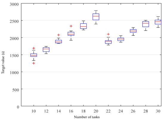
Figure A1.
A boxplot for all the objective values for the solution of the small-sized cases by [M1] (units: s).
Appendix B. Comparison of Computing Performance of RSA and ALNS as the Number of Iterations Increases
Table A3.
Computing performance of RSA and ALNS (the units for , , and are seconds).
Table A3.
Computing performance of RSA and ALNS (the units for , , and are seconds).
| No. of Tasks | RSA | ALNS | ||||
|---|---|---|---|---|---|---|
| a | ||||||
| 10 | 1548 | 0.0 | <0.01 | 1548 | 1548 | 0.93 |
| 12 | 1742 | 0.0 | <0.01 | 1742 | 1792 | 0.19 |
| 14 | 2000 | 0.2 | <0.01 | 1996 | 2128 | 0.34 |
| 16 | 2132 | 1.4 | <0.01 | 2102 | 2275 | 0.39 |
| 18 | 2385 | 4.8 | <0.01 | 2275 | 2604 | 0.52 |
| 20 | 2769 | 13.7 | <0.01 | 2435 | 2837 | 0.69 |
| 22 | 1833 | 0.0 | <0.01 | 1833 | 1878 | 0.51 |
| 24 | 1951 | 0.0 | <0.01 | 1951 | 2029 | 0.45 |
| 26 | 2160 | 0.0 | <0.01 | 2160 | 2309 | 0.48 |
| 28 | 2430 | 0.3 | <0.01 | 2423 | 2503 | 0.50 |
| 30 | 2566 | 5.4 | <0.01 | 2435 | 2654 | 0.34 |
| 32 | 1929 | 0.0 | <0.01 | 1929 | 2028 | 1.34 |
| 34 | 2166 | 3.0 | <0.01 | 2102 | 2249 | 0.81 |
| 36 | 2173 | 2.4 | <0.01 | 2122 | 2237 | 1.25 |
| 38 | 2246 | 0.6 | <0.01 | 2233 | 2335 | 0.43 |
| 40 | 2580 | 5.6 | <0.01 | 2442 | 2645 | 2.20 |
| 50 | 2344 | 3.6 | <0.01 | 2263 | 2430 | 1.95 |
| 60 | 3489 | 6.8 | <0.01 | 3268 | 3617 | 1.36 |
| 70 | 4192 | 5.6 | <0.01 | 3970 | 4397 | 2.78 |
| 80 | 5075 | 11.3 | <0.01 | 4559 | 5210 | 1.95 |
| 90 | 5546 | 7.6 | <0.01 | 5156 | 5674 | 3.11 |
| 100 | 6384 | 6.9 | <0.01 | 5970 | 6680 | 4.43 |
| 110 | 7224 | 9.9 | <0.01 | 6573 | 7663 | 4.12 |
| 120 | 7415 | 9.9 | <0.01 | 6750 | 7641 | 3.84 |
| 130 | 8200 | 7.1 | <0.01 | 7654 | 8470 | 4.10 |
| 140 | 9064 | 9.2 | <0.01 | 8300 | 9298 | 5.52 |
| 150 | 9646 | 7.6 | <0.01 | 8964 | 10,084 | 5.22 |
| 160 | 10,939 | 6.6 | <0.01 | 10,264 | 11,499 | 5.86 |
a This value was calculated as follows: . The number of RSA iterations is set to , and the number of ALNS iterations is set to .
Appendix C. Comparison of Computing Performance of ALNS and GA
Table A4.
Computing performance of GA and ALNS (the units for , , and are seconds).
Table A4.
Computing performance of GA and ALNS (the units for , , and are seconds).
| No. of Tasks | GA | ALNS | ||||
|---|---|---|---|---|---|---|
| a | ||||||
| 10 | 1548 | 0.00 | 1.17 | 1548 | 1548 | 0.93 |
| 12 | 1742 | 0.00 | 1.15 | 1742 | 1754 | 0.31 |
| 14 | 1997 | 0.00 | 1.27 | 1997 | 2019 | 0.19 |
| 16 | 2202 | 2.72 | 1.66 | 2144 | 2227 | 0.95 |
| 18 | 2433 | 6.93 | 1.40 | 2275 | 2301 | 0.40 |
| 20 | 2656 | 9.11 | 1.41 | 2435 | 2566 | 0.58 |
| 22 | 1833 | −2.88 | 1.87 | 1887 | 1889 | 0.42 |
| 24 | 1999 | 2.49 | 1.45 | 1951 | 1969 | 0.55 |
| 26 | 2265 | 4.89 | 1.98 | 2160 | 2236 | 0.72 |
| 28 | 2457 | 1.39 | 1.48 | 2423 | 2446 | 0.36 |
| 30 | 2601 | 6.83 | 1.56 | 2435 | 2506 | 0.86 |
| 32 | 1981 | 0.89 | 2.29 | 1964 | 1984 | 0.91 |
| 34 | 2133 | 1.44 | 2.53 | 2102 | 2117 | 1.39 |
| 36 | 2217 | 4.51 | 2.48 | 2122 | 2195 | 1.50 |
| 38 | 2300 | 0.74 | 1.70 | 2283 | 2315 | 0.40 |
| 40 | 2577 | 5.53 | 3.04 | 2442 | 2544 | 2.23 |
| 50 | 2366 | 3.52 | 2.73 | 2285 | 2330 | 1.39 |
| 60 | 3456 | 4.47 | 2.08 | 3308 | 3410 | 1.36 |
| 70 | 4227 | 6.50 | 3.41 | 3970 | 4278 | 3.03 |
| 80 | 5019 | 10.09 | 3.76 | 4559 | 4892 | 3.01 |
| 90 | 5511 | 6.87 | 3.98 | 5156 | 5305 | 3.26 |
| 100 | 6478 | 8.51 | 5.30 | 5970 | 6272 | 5.00 |
| 110 | 7376 | 12.21 | 4.71 | 6573 | 6742 | 4.64 |
| 120 | 7247 | 7.35 | 4.93 | 6750 | 6980 | 4.11 |
| 130 | 8262 | 7.70 | 4.97 | 7672 | 7874 | 4.59 |
| 140 | 9133 | 10.03 | 6.27 | 8300 | 8576 | 6.18 |
| 150 | 9882 | 8.87 | 6.35 | 9077 | 9409 | 5.61 |
| 160 | 11,002 | 6.29 | 5.44 | 10,351 | 10,831 | 5.37 |
a This value was calculated as follows:
Information Related to Genetic Algorithm
The random key encoding method is used to determine the order of ARMG job tasks, and the decoding and fitness value can be solved by referring to Section 5.1;
Roulette wheel selection procedure;
Scattered crossover operator;
Uniform mutation operator;
Population size = 40;
Largest number of iterations = 500;
Crossover probability = 0.8;
Mutation probability = 0.2;
Generation of initial population: Following an initial solution by RSA, another sequence is randomly generated.
References
- Zhao, W.; Zhang, D.; Zou, Y. Technological Analysis of Automatic Container Terminal Automated Guided Vehicle and Intelligent Guided Vehicle. J. Phys. Conf. Ser. 2021, 2033, 012207. [Google Scholar] [CrossRef]
- Chu, F.; He, J.; Zheng, F.; Liu, M. Scheduling multiple yard cranes in two adjacent container blocks with position-dependent processing times. Comput. Ind. Eng. 2019, 136, 355–365. [Google Scholar] [CrossRef]
- Luo, J.; Wu, Y.; Mendes, A.B. Modelling of integrated vehicle scheduling and container storage problems in unloading process at an automated container terminal. Comput. Ind. Eng. 2016, 94, 32–44. [Google Scholar] [CrossRef]
- Xiang, X.; Liu, C. Modeling and analysis for an automated container terminal considering battery management. Comput. Ind. Eng. 2021, 156, 107258. [Google Scholar] [CrossRef]
- Cao, Y.; Yang, A.; Liu, Y.; Zeng, Q.; Chen, Q. AGV dispatching and bidirectional conflict-free routing problem in automated container terminal. Comput. Ind. Eng. 2023, 184, 109611. [Google Scholar] [CrossRef]
- Yang, X.; Hu, H.; Jin, J. Battery-powered automated guided vehicles scheduling problem in automated container terminals for minimizing energy consumption. Ocean Coast. Manag. 2023, 246, 106873. [Google Scholar] [CrossRef]
- Oladugba, A.O.; Gheith, M.; Eltawil, A. A new solution approach for the twin yard crane scheduling problem in automated container terminals. Adv. Eng. Inform. 2023, 57, 102015. [Google Scholar] [CrossRef]
- Gao, Y.; Chang, D.; Chen, C.-H. A digital twin-based approach for optimizing operation energy consumption at automated container terminals. J. Clean. Prod. 2023, 385, 135782. [Google Scholar] [CrossRef]
- Hu, H.; Huang, Y.; Zhen, L.; Lee, B.K.; Lee, L.H.; Chew, E.P. A decomposition method to analyze the performance of frame bridge based automated container terminal. Expert Syst. Appl. 2014, 41, 357–365. [Google Scholar] [CrossRef]
- Kaveshgar, N.; Huynh, N. Integrated quay crane and yard truck scheduling for unloading inbound containers. Int. J. Prod. Econ. 2015, 159, 168–177. [Google Scholar] [CrossRef]
- Skaf, A.; Lamrous, S.; Hammoudan, Z.; Manier, M.-A. Integrated quay crane and yard truck scheduling problem at port of Tripoli-Lebanon. Comput. Ind. Eng. 2021, 159, 107448. [Google Scholar] [CrossRef]
- Hop, D.C.; Van Hop, N.; Anh, T.T.M. Adaptive particle swarm optimization for integrated quay crane and yard truck scheduling problem. Comput. Ind. Eng. 2021, 153, 107075. [Google Scholar] [CrossRef]
- Liu, W.; Zhu, X.; Wang, L.; Wang, S. Multiple equipment scheduling and AGV trajectory generation in U-shaped sea-rail intermodal automated container terminal. Measurement 2023, 206, 112262. [Google Scholar] [CrossRef]
- Luo, J.; Wu, Y. Modelling of dual-cycle strategy for container storage and vehicle scheduling problems at automated container terminals. Transp. Res. Part E Logist. Transp. Rev. 2015, 79, 49–64. [Google Scholar] [CrossRef]
- Wang, Y.-Z.; Hu, Z.-H.; Tian, X.-D. Scheduling ASC and AGV considering direct, buffer, and hybrid modes for transferring containers. Comput. Oper. Res. 2024, 161, 106419. [Google Scholar] [CrossRef]
- Zhang, X.; Li, H.; Sheu, J.-B. Integrated scheduling optimization of AGV and double yard cranes in automated container terminals. Transp. Res. Part B Methodol. 2024, 179, 102871. [Google Scholar] [CrossRef]
- Zhang, C.; Liu, J.; Wan, Y.-w.; Murty, K.G.; Linn, R.J. Storage space allocation in container terminals. Transp. Res. Part B Methodol. 2003, 37, 883–903. [Google Scholar] [CrossRef]
- Skinner, B.; Yuan, S.; Huang, S.; Liu, D.; Cai, B.; Dissanayake, G.; Lau, H.; Bott, A.; Pagac, D. Optimisation for job scheduling at automated container terminals using genetic algorithm. Comput. Ind. Eng. 2013, 64, 511–523. [Google Scholar] [CrossRef]
- He, J.; Huang, Y.; Yan, W.; Wang, S. Integrated internal truck, yard crane and quay crane scheduling in a container terminal considering energy consumption. Expert Syst. Appl. 2015, 42, 2464–2487. [Google Scholar] [CrossRef]
- Yang, Y.; Zhong, M.; Dessouky, Y.; Postolache, O. An integrated scheduling method for AGV routing in automated container terminals. Comput. Ind. Eng. 2018, 126, 482–493. [Google Scholar] [CrossRef]
- Zhong, M.; Yang, Y.; Dessouky, Y.; Postolache, O. Multi-AGV scheduling for conflict-free path planning in automated container terminals. Comput. Ind. Eng. 2020, 142, 106371. [Google Scholar] [CrossRef]
- Luo, J.; Wu, Y. Scheduling of container-handling equipment during the loading process at an automated container terminal. Comput. Ind. Eng. 2020, 149, 106848. [Google Scholar] [CrossRef]
- Shouwen, J.; Di, L.; Zhengrong, C.; Dong, G. Integrated scheduling in automated container terminals considering AGV conflict-free routing. Transp. Lett. 2020, 13, 501–513. [Google Scholar] [CrossRef]
- Xu, B.; Jie, D.; Li, J.; Yang, Y.; Wen, F.; Song, H. Integrated scheduling optimization of U-shaped automated container terminal under loading and unloading mode. Comput. Ind. Eng. 2021, 162, 107695. [Google Scholar] [CrossRef]
- Niu, Y.; Yu, F.; Yao, H.; Yang, Y. Multi-equipment coordinated scheduling strategy of U-shaped automated container terminal considering energy consumption. Comput. Ind. Eng. 2022, 174, 108804. [Google Scholar] [CrossRef]
- Yue, L.-J.; Fan, H.-M.; Fan, H. Blocks allocation and handling equipment scheduling in automatic container terminals. Transp. Res. Part C Emerg. Technol. 2023, 153, 104228. [Google Scholar] [CrossRef]
- Yu, M.; Liu, X.; Xu, Z.; He, L.; Li, W.; Zhou, Y. Automated rail-water intermodal transport container terminal handling equipment cooperative scheduling based on bidirectional hybrid flow-shop scheduling problem. Comput. Ind. Eng. 2023, 186, 109696. [Google Scholar] [CrossRef]
- Li, J.; Yan, L.; Xu, B. Research on Multi-Equipment Cluster Scheduling of U-Shaped Automated Terminal Yard and Railway Yard. J. Mar. Sci. Eng. 2023, 11, 417. [Google Scholar] [CrossRef]
- He, J.; Zhang, L.; Deng, Y.; Yu, H.; Huang, M.; Tan, C. An allocation approach for external truck tasks appointment in automated container terminal. Adv. Eng. Inform. 2023, 55, 101864. [Google Scholar] [CrossRef]
- Zhen, L.; Hu, H.; Wang, W.; Shi, X.; Ma, C. Cranes scheduling in frame bridges based automated container terminals. Transp. Res. Part C Emerg. Technol. 2018, 97, 369–384. [Google Scholar] [CrossRef]
- Yang, Y.; He, S.; Sun, S. Research on the Cooperative Scheduling of ARMGs and AGVs in a Sea–Rail Automated Container Terminal under the Rail-in-Port Model. J. Mar. Sci. Eng. 2023, 11, 557. [Google Scholar] [CrossRef]
- Yang, Y.; Sun, S.; He, S.; Jiang, Y.; Wang, X.; Yin, H.; Zhu, J. Research on the Multi-Equipment Cooperative Scheduling Method of Sea-Rail Automated Container Terminals under the Loading and Unloading Mode. J. Mar. Sci. Eng. 2023, 11, 1975. [Google Scholar] [CrossRef]
- Chen, H.; Liu, W. An Adaptive Large Neighborhood Search Algorithm for Equipment Scheduling in the Railway Yard of an Automated Container Terminal. J. Mar. Sci. Eng. 2024, 12, 710. [Google Scholar] [CrossRef]
- Aslam, S.; Michaelides, M.P.; Herodotou, H. Berth Allocation Considering Multiple Quays: A Practical Approach Using Cuckoo Search Optimization. J. Mar. Sci. Eng. 2023, 11, 1280. [Google Scholar] [CrossRef]
- Aksen, D.; Kaya, O.; Sibel Salman, F.; Tüncel, Ö. An adaptive large neighborhood search algorithm for a selective and periodic inventory routing problem. Eur. J. Oper. Res. 2014, 239, 413–426. [Google Scholar] [CrossRef]
- Ropke, S.; Pisinger, D. An Adaptive Large Neighborhood Search Heuristic for the Pickup and Delivery Problem with Time Windows. Transp. Sci. 2006, 40, 455–472. [Google Scholar] [CrossRef]
- Zhang, Y.; Atasoy, B.; Negenborn, R.R. Preference-Based Multi-Objective Optimization for Synchromodal Transport Using Adaptive Large Neighborhood Search. Transp. Res. Rec. J. Transp. Res. Board 2021, 2676, 71–87. [Google Scholar] [CrossRef]
- Zhang, Y.; Li, X.; van Hassel, E.; Negenborn, R.R.; Atasoy, B. Synchromodal transport planning considering heterogeneous and vague preferences of shippers. Transp. Res. Part E Logist. Transp. Rev. 2022, 164, 102827. [Google Scholar] [CrossRef]
- Wu, Y.; Qureshi, A.G.; Yamada, T. Adaptive large neighborhood decomposition search algorithm for multi-allocation hub location routing problem. Eur. J. Oper. Res. 2022, 302, 1113–1127. [Google Scholar] [CrossRef]
- Chang, X.; Shi, J.; Luo, Z.; Liu, Y. Adaptive large neighborhood search algorithm for multi-stage weapon target assignment problem. Comput. Ind. Eng. 2023, 181, 109303. [Google Scholar] [CrossRef]
- Shi, J.; Mao, H.; Zhou, Z.; Zheng, L. Adaptive large neighborhood search algorithm for the Unmanned aerial vehicle routing problem with recharging. Appl. Soft Comput. 2023, 147, 110831. [Google Scholar] [CrossRef]
- Sun, P.; Veelenturf, L.P.; Hewitt, M.; Van Woensel, T. Adaptive large neighborhood search for the time-dependent profitable pickup and delivery problem with time windows. Transp. Res. Part E Logist. Transp. Rev. 2020, 138, 101942. [Google Scholar] [CrossRef]
- Wang, X.; Liang, Y.; Wei, X.; Chew, E.P. An adaptive large neighborhood search algorithm for the tugboat scheduling problem. Comput. Ind. Eng. 2023, 177, 109039. [Google Scholar] [CrossRef]
Disclaimer/Publisher’s Note: The statements, opinions and data contained in all publications are solely those of the individual author(s) and contributor(s) and not of MDPI and/or the editor(s). MDPI and/or the editor(s) disclaim responsibility for any injury to people or property resulting from any ideas, methods, instructions or products referred to in the content. |
© 2024 by the authors. Licensee MDPI, Basel, Switzerland. This article is an open access article distributed under the terms and conditions of the Creative Commons Attribution (CC BY) license (https://creativecommons.org/licenses/by/4.0/).