1. Introduction
The Global Sulphur Cap (GSC) has led to a drastic reduction in permitted emissions in global shipping. Thus, since January 2020, outside of emission control areas (ECA), a maximum of 0.5%S fuels is allowed; with this content being reduced to 0.1%S for ECA zones (Annex VI of MARPOL 73/78). In a further step, several recent communications within the European Green Deal context (COM (2021) 551 final, COM (2021) 562 final and COM (2021) 563 final), have signaled imminent Market-Based Measures (MBM), which will come into force to improve European shipping’s environmental performance.
These normative developments involve a serious challenge for operators of Short Sea Shipping (SSS) vessels, who must meet not only more stringent regulations, but also have to keep the SSS service economic in comparison to other transport modes. Consequently, in the last decade, numerous studies have focused on the techno-economic optimization of liner traffic vessels and their operation [
1,
2,
3,
4,
5,
6,
7,
8,
9] which include sizing, propulsion alternatives, optimal speed, abatement systems, or port supply energy, by ensuring the competitiveness of the transport service and fulfilling the requirements of the environmental normative.
Among the previously mentioned optimization parameters, the one mostly related to fuel consumption and, subsequently, with emissions, is the ship propulsion power demand, which is largely related to calm water resistance, propeller efficiency, and prevailing weather conditions (which induce added resistance in waves and other relevant resistance components, such as those due to wind or current).
Considering that these types of optimization process, not only during ship design but also for ship routing, usually require evaluation of a large number of alternatives, the use of simplified models and the non-consideration of some components is a common method of approaching these problems. In this respect, previous studies, focused on vessel optimization at design stages and route optimization, have mostly estimated vessel resistance through standard simplified prediction methods, without carefully considering their accuracy. For example, in [
7], the authors optimize ship propellers for reducing fuel consumption by taking into consideration only calm water resistance, estimated using the Holtrop–Mennen method. In [
8], a more complete proposal for estimating fuel use is presented, including also the influence of added resistance in waves, motions or wind in addition to calm water resistance. However, again calm water resistance is estimated using the Hotrop–Mennen approach.
Although such proposals could represent a good approach for the comparison of different alternative designs (or routes), the implicit uncertainty in the estimation of calm water resistance has not been addressed in the optimizations. This is because, even though broad awareness exists about the implications of this misestimation, wrong air emissions, erroneous operational costs, OPEX, etc., occur.
In parallel, numerous studies have focused on vessel speed optimization ([
1,
10,
11], among others) as a relevant measure to mitigate air emissions and moderate OPEX for SSS. Indeed, most of these studies—Operations Research and Maritime Economics—establish simple relationships between fuel consumption (SFOC) and vessel speed by adopting a second-level approach (operative strategy [
12]). This involves taking preliminary steps (for instance, a cubic fuel consumption function regarding sailing speed, and therefore the required power [
1,
10]) to evaluate the operational performance of existing vessels (tactic analysis). Again, the vessels’ resistance at a particular speed, that is, the technological strategy (first-level approach [
12]) has not sufficiently considered the possible consequences of this lack of accuracy in this research line.
In light of the above, this paper attempts to provide quantitative information about the environmental implications of a possible lack of accuracy in the estimation of SSS vessel resistance, specifically in the estimation of calm water resistance. To achieve this, the paper analyzes and compares the resistance predictions for an SSS vessel (an optimized feeder vessel) obtained using estimation methods with increasing accuracy levels. These include a simplified early decision-making tool (J. Mau method), a widely used semi-empirical method (Holtrop–Mennen), and Computational Fluid Dynamics (CFD) simulations, which represent the state-of-the-art tool for estimating ship resistance in calm water and which could obtain, in many cases, very good approximations to the results of towing tank tests [
13].
The results of this analysis are shown in monetary terms regarding the consequent air emissions. This provides useful insights for uncertainty management in further research and for policy-making purposes.
2. Method
The first step in defining propulsion power for vessel optimization is prediction of resistance. This section considers three prediction methods that have increasing accuracy: the first approach method, simply based on each vessel’s main features; the second approach method, where hull performance is primarily estimated through non-dimensional coefficients, and finally, an ad hoc analysis for a particular hull model, where the model is fully evaluated through CFD.
The application of all these methods to a particular vessel allows us to determine the uncertainties assumed when empirical methods are applied to full-scale predictions of a vessel’s resistance in optimization processes.
2.1. J. Mau
D.G.M. Watson and J. Mau’s methods [
14,
15], among other expressions, are classic early decision-making tools commonly used for a first approach estimation of the required propulsion power for vessels at a particular speed (initial design stage). This is because their application only requires knowledge of a limited number of key features. This is especially useful when detailed data about the hull shape, for example, are not clearly established or not available. For the same reason, they are predominantly used in optimization processes that employ mathematical models [
4,
16], among others where high numbers of variables are simultaneously handled. The application of these methods in an optimization context permits computational time to be reduced by simplifying the models. However, these equations are inaccurate as they consider the towing tank test results of a vessels’ database at particular speeds, and then relate these results to the vessel’s main dimensions.
It is therefore recommended that these expressions are adapted from cargo ships with a deadweight below 15,000 tonnes to the range of vessels that will be specifically evaluated (update methods). This is because, among other assumptions, these expressions are based on hull shapes and tank test methods at a particular time [
15]. In this process, corrective coefficients are included in the general expressions to improve the estimations and actualize the methods. Therefore—with knowledge of the real required power for vessels in a particular range—corrected coefficients are obtained by applying the expressions and adjusting them to real powers.
Expression 1 shows the equation for the power estimation (
BHP in HP units) for a main engine with a corrective coefficient for SSS vessels (small and fast ships). Expression 2 provides the coefficient calculation (
Coef) by considering the Froude Number (
Fr) of the evaluated vessels (Feeder vessel for SSS traffic published by the
Significant Ships journal
1 between 1994 and 2008).
where:
Δ: displacement at design draft (tons).
VB: service speed (kn).
The corrective coefficient was obtained by considering BHPs and service speeds for feeder vessels in SSS traffic. Consequently, expression 1 is suitable to obtain BHP at a particular service speed for this vessel range and was applied in the optimization processes for these types of vessels [
4,
5,
16].
2.2. Holtrop and Mennen’s Method
This popular expression for the estimation of a vessel’s resistance has been widely used by naval architects since 1984 [
17,
18], although it was later updated. The expression draws on an experimental towing-tank regression analysis from numerous Netherlands Ship Model Basin (MARIN) results and full-scale ship data, and provides an estimation of different resistance components by considering hull performance, mainly (see Equation (3)): form factor, wave-making resistance coefficient, appendage resistance coefficient, additional pressure resistance of a bulbous bow, additional pressure resistance due to immersed transom stern and the coefficient of model–vessel correlation resistance. These coefficients are based on the waterline length, the draught, non-dimensional coefficients such as block coefficient, and other similar dimensions and coefficients that do not evaluate specific aspects of the hull, such as turbulence [
17,
18].
This method divides ship resistance as follows:
where:
is frictional resistance according to the ITTC—1957 friction formula.
(1 + k1) is the form factor.
is the appendage resistance.
is wave resistance.
is the bulbous bow additional pressure resistance.
is the transom stern resistance.
is the model–ship correlation resistance.
While Holtrop–Mennen has been a useful and widely used predicting method for the resistance of several types of hull forms and sizes (tankers, general cargo ships, container ships, etc.), the method is only useful within certain speed ranges (Frmax = 0.80).
2.3. Computational Fluid Dynamics (CFD) Analysis
CFD is currently one of the most important approaches used in hydrodynamics for researching naval and industrial issues. In most hydrodynamic problems, not only in ships but also in the offshore structure sector, the presence of complex flow along the submerged body makes the use of computational tools for calculating the various equations essential. Jasak, H. (2009) [
19] describes one of those numerical tools, known as OpenFOAM
2, and succinctly demonstrates how it is employed to address fluid dynamics’ problems.
The open-source code OpenFOAM is used for multiple purposes in fluid dynamics, such as studying the effects of the free surface in an elastic beam [
20] or the effect of Vortex-Induced Vibrations (VIV) [
21]. These studies use canonical calculations, so that more complex geometries can be identified, such as in the research of Moran-Guerrero et al., 2018 [
22], where turbulence transition in a ship propeller is treated. These examples show the importance of CFD since it can help to clarify the fluid flow effects in a new geometry, like that proposed in [
23] which cannot be evaluated with statistical methods.
OpenFOAM was employed to address this problem, and it has subsequently been widely used for ship resistance calculations, with good results ([
13], among others]). Thus, CFD methods have also been widely used for other vessels with very different technical features: amphibious craft [
24], fast craft [
25], and commercial ships. Thus, in [
26,
27] statistical methods have been compared, such as that of Holtrop and Mennen, with CFD. Their study concludes that CFD can provide more details about flow behavior that cannot be obtained by traditional studies only offering a resistance curve. Therefore, a detailed study of fluid flow behavior and ship resistance can be used in innovative design methodologies, such as that proposed in [
23].
When a CFD code is used, all previous works are taken into account, together with some prior recommendations such as: those proposed by the ITTC [
28] by including ship turbulence [
29], the importance of timestep and mesh size [
30], and the different effects of boundaries in CFD simulations [
31].
Hence, the open-source code OpenFOAM, that implements the Finite Volume Method (FVM), is used as a computing tool for obtaining the ship resistance. The well-known Navier–Stokes equations will be solved (see Equations (4) and (5)) for the fluid phases. The different variables are: ‘p’ is the pressure field,
uf is the fluid velocity vector,
μf is the fluid viscosity, and
ρf the fluid density.
A transient PISO algorithm (Pressure-Implicit with Splitting of Operators) [
32,
33] is used to solve non steady Navier–Stokes’ equations.
The assessment of SSS vessel resistance was assumed to be a multi-phase case, therefore, the Volume of Fluid (VOF) method is used. Equation (6) models the volume fraction of one phase α, that is a scalar fraction that will define in each cell the fluid that is inside.
Previous equations are complemented with the two equations, the turbulence kinetic energy, k, and turbulence specific dissipation rate Ω, in a k-Omega-SST model (SST k-omega model 3, s.f.) This Reynolds averaged Navier–Stokes method (RANS) is used to model turbulence in the present study.
2.4. Estimation Method for the Environmental Costs
The assessment of pollutant air emissions is based on a modification of the model published in [
4]. The modified model includes the evaluation of PM
10 as a pollutant and does not consider the berthing stage for the assessment. Even though significant environmental advantages for SSS can be achieved through OPS (on shore power supply) during the berthing time [
5], especially in regions with a high RES (renewable energy sources) share [
34], the berthing time was excluded in the model because the analysis of this work is focused on the vessel’s resistance prediction and during the berthing time (mooring and loading/unloading operations) the vessel speed is zero.
Moreover, the model was adapted to the current analysis by offering environmental information per trip (
CEM in EUR/trip, see Equation (7)).
Equations (7)–(10) show the environmental assessment in monetary terms of the pollutant air emissions, where the navigation stages (S = {1, …, s}), free sailing, and maneuvering (time from arriving at the port area—fairway buoy—to the berth), are considered jointly. The model assesses the following pollutants (U = {1, …, u}): SO2 (acidifying substances), NOx (ozone precursors), PM2.5, PM10 (particular matter mass), and the greenhouse gases CO2 and CH4. The environmental impact of these pollutants is conditioned by the geographical localization of the emissions (countries or seas F = {1, …, f}) and the localization’s population (V = {1, …, v}): rural zone, city, or metropole.
The calculation method considers the emission factors per pollutant for every navigation stage (EGsu; ∀s∈S∧∀u∈U in kg/h), the unitary costs (CFsufv; ∀s ∈ S∧∀u ∈ U∧∀f ∈ F∧∀v ∈ V in EUR/kg), and the time invested at every navigation stage (TVBs; ∀s ∈ S).
All emission factors are taken from the calculation tools developed by the Technical University of Denmark
4 [
35,
36]. However, since this tool does not provide desegregated emission factors for particulate matter mass, the relationship between PM
2.5 and PM
10 emissions published by the ‘
EMEP/EEA air pollutant emission inventory guidebook, 2019’—for several fuels—was considered to obtain the emission factors for these pollutants.
Likewise, the CH
4 emission factor is not provided by the calculation tool from the Technical University of Denmark [
35,
36]. Consequently, the CH
4 emissions are evaluated in monetary terms, according to the calculation method proposed by the United States Environmental Protection Agency (US EPA) [
37]. This method (see Equations (2) and (4)) considers the load factor of the engine at each seaborne stage (LF
s; ∀s ∈ SS), the propulsion power of the vessels (
PB in kW), and the CH
4 emission factor (
EF) provided by the propulsion plant evaluated. According to previous research in this regard, EF = 5.79 g/kWh for dual engines operating with LNG [
3,
38].
The unitary costs for the pollutants (
CFsufv; ∀s ∈ S∧∀u ∈ U∧∀f ∈ F∧∀v ∈ V in EUR/kg pollutant) were taken from the
Handbook on the External Costs of Transport (last updated in 2019) [
39], published by the European Commission. These values are updated according to the Consumer Price Index (CPI) for the countries involved in the transport. In fact, in the free sailing stage (see Equation (4)), the unitary cost and the emission factor are not dependent on population density or the country (∀f ∈ F∧∀v ∈ V—see Equation (2)). In turn, the climate change avoidance cost (central value) was taken for CO
2. Finally, the CH
4 emission cost is estimated as a function of its Global Warning Potential (GWP), by assuming GWP = 1 for CO
2 and GWP = 25 for CH
4 [
4,
40].
3. Application Case
In order to address the environmental consequences of the deviations among the resistance prediction methods, these were applied to a particular case.
Through the optimization carried out in [
4], a feeder fleet was obtained to operate under SSS conditions in the Atlantic coast between Spain and France (Vigo-St. Nazaire). The main features of these vessels, obtained through a multi-objective algorithm (the minimization of the environmental costs, minimization of operative cost, and the minimization of the time invested in the travel were the three objective functions), were assumed as a base case for the analysis (see
Table 1). Fleet results were found by assuming J. Mau’s method (see Equations (1) and (2)) to evaluate the required power for the vessels at the design draught. As expected, to offer a competitive intermodal option versus the trucking alternative, the vessels were found to be small and especially fast (19.49 kn for service speed at the design draught, see
Table 1); likewise, dual engines were found to be the most suitable propulsion alternative for the fleet. It is worth bearing in mind that the average service speed for vessels of these dimensions is 11 kn (for example: “JA SONG 2”—IMO number 9000766; “KM SAMUDERA MAS”—IMO number 9069944, etc.).
The hull of the feeder vessel obtained in the optimization process was modeled in 3D. This model was introduced in the CFD, OpenFOAM, and the hull resistance was computed through the numerical methods. Parallelly, the resistance estimation for the vessel was calculated using the Holtrop method.
In this case study, the CPI (from January 2016–2021) of Spain (Spanish Statistical Office, 6.2%) and France (National Institute of Statistics and Economic Studies of France, 0.4), were applied to update the unitary costs for the pollutants provided by the
Handbook on the External Costs of Transport [
40]. Since St. Nazaire and Vigo’s hinterlands have populations below 0.5 million inhabitants, all costs will refer to urban zones (V = {1, …,
v}-rural, urban, or metropolitan areas).
The maritime distance between Vigo and St. Nazaire port (464 nautical miles) and their port performance have led to the assumption of operation times: TVB
2 = 20 min (maneuvering time per port) and TVB
1 = 23.8 h (sailing time at service speed of 19.49 kn, see
Table 1). Regarding the latter, it is interesting to stress the time difference in comparison to a conventional speed (TVB
1 = 42.18 h for 11 kn of service speed).
Problem Description for the CFD Application
The application case was assumed as the hull resistance analysis in an incompressible flow. The mesh used is presented in
Figure 1. The reference point for measuring the distances to the boundaries was the forward perpendicular.
Taking the forward perpendicular as the reference the following distances were used for defining the boundary distances; inlet 2.5 L, outlet 5 L, bottom 3 L, top 2.5 L, and back 3 L, where L is the length of the ship.
Since the application case is a three-dimensional problem and ship symmetry exists, a periodic boundary condition was used. The flow comes from the bow to stern in a calm water resistance study with a ship specification (see
Table 1).
A time step convergence and a mesh convergence were performed in order to evaluate the dependency on the result (see
Table 2). The convergence was reached for the data presented in
Table 1. The mesh was created with the utility snappyHexMes and different hexahedral meshes were evaluated. The mesh near the free surface was refined (see
Figure 2) to avoid numerical divergences. The boundary layer around the ship was set at six layers to ensure a good resolution.
Different time steps were also evaluated to ensure numerical convergence. Due to the low error between cases, it can be assumed that mesh and time step convergence were fulfilled. Therefore, according to
Table 2, any proposed set up could be used due to the low error between them. Nonetheless, case 3 was used throughout this study, since it involves an intermediate configuration, bigger time step, and more cell numbers.
4. Results
Table 3 presents the resistance and propulsion power of the base case, the optimized vessel, when the vessel is operating in different navigation stages. Likewise, the table shows the results obtained for free sailing when the vessel operates at a conventional speed (11 kn), instead of the optimized speed (19.49 kn). In order to compare the results for the selection of the main engine by assuming the free sailing stage, the required Effective Horse Power (
EHP), Break House Power (
BHP), and the Maximum Continuous Rating (
MCR) were calculated from the resistance (Holtrop and CFD results) and
BHP estimation (see Equations (1) and (2) for J. Mau’s method) according to Expressions (11) and (12).
where the following values were assumed in all cases [
35,
41]:
SM: sea margin = 15%.
EM: engine margin = 10%.
: hull efficiency = 0.919.
: propeller open water efficiency = 0.631 for free sailing and 0.395 for manouvering stage.
: relative rotative efficiency = 1.010.
: mechanical efficiency = 0.97.
It is important to note that, for calculating
BHP through the Holtrop method and CFD simulations, it is necessary to assume propulsion coefficients (as shown above); whereas through J. Mau, this step is already considered within the method (and no explicit propulsive coefficients are applied). Consequently, a small percentage of the differences between the estimations (J. Mau, Holtrop and CFD, see
Figure 3) may be due to this factor.
Figure 3 shows the performance of the resistance prediction methods when the operation speed changes in the vessel. Even though all power curves fit well (R
2 close to 1) to cubic relationships with the speed, notable differences exist among them for speeds over 15.5 kn. In addition, J. Mau shows an overestimation between 7 and 15.5 knots in relation to the other methods for the feeder analyzed.
Consequently, the optimized vessels using the J. Mau method will provide better environmental performance than expected when the service speed reached by the optimization process is below 15.5 kn; whereas it will be the opposite for higher service speeds. In turn, Holtrop and CFD methods have proven to offer similar performance up to 15.5 kn. For speeds higher than 15.5 kn, a misestimation exists in the Holtrop method.
Deviations and Discussion
Figure 4,
Figure 5,
Figure 6 and
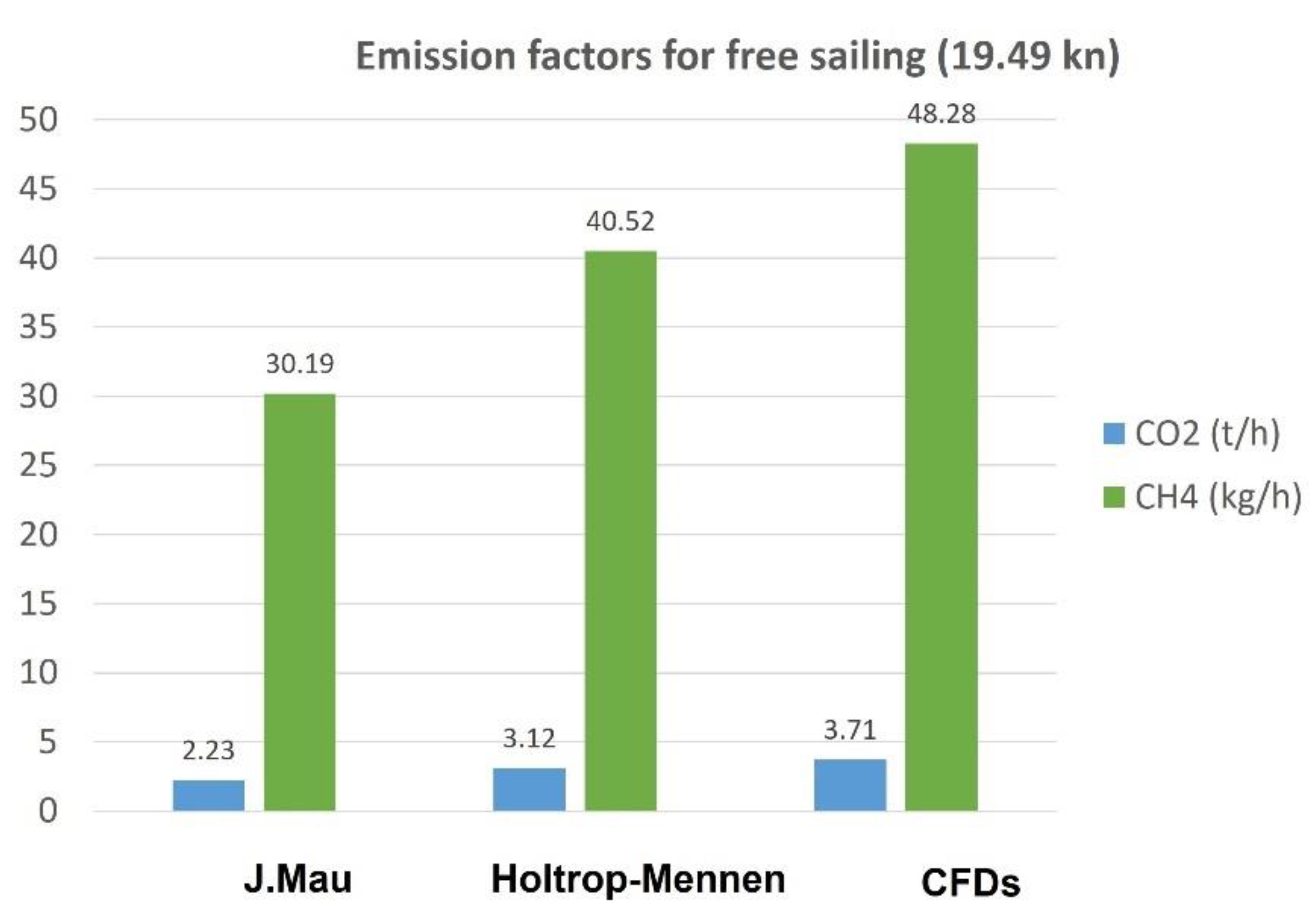
Figure 7 show the emission factors obtained for the feeder vessels (see
Table 1) when the vessels’ resistance is taken from the different estimation methods. Dual engines assume the integration of the SCR—Selective Catalyic Reduction system—as they specify NO
x reduction technology for operating with liquid fuel (Tier-III engines).
The deviations found for the emission factors are relevant for all pollutants by sailing at an optimized speed (19.49 kn, see
Figure 4 and
Figure 5). In this scenario, all methods offer lower emission factors than CFD. Thus, by using the J. Mau method the average deviation of emission factors regarding CFD reaches −37%. Likewise, the Holtrop method provides misestimations up to −18% on CFD emission factors.
Figure 6 and
Figure 7 show the emission factor differences when the service speed of the vessel is 11 kn (conventional speed) instead of 19.49 kn (optimized speed). In contrast to the deviations found when the service speed is the optimized one, in this scenario the deviations are positive with regard to CFD emission factors (as expected according to
Figure 3). Again, the deviation provided by J. Mau is especially notable by reaching 80%, whereas the Holtrop method provides an average deviation of 6.5% for the emission factors.
In the maneuvering stage the deviations for the emission factors are more moderated, as expected (see
Figure 3), by being this positive and practically constant in all scenarios: 4% for Holtrop and 18% for J. Mau emission factors if compared with CFD results.
Table 4 presents the deviations in terms of required power and environmental cost with
CEM being the environmental costs (see Equations (7)–(10)) when the different methods are applied and compared to CFD results, which are assumed to be the most accurate. More than −16% deviation was found for the required power when the Holtrop method was used at the free sailing stage, whereas −39.21% was reached when the J. Mau simulations were carried out. Positive deviations were obtained by both methods (J. Mau and Holtrop) when the maneuvering stage was evaluated (18.85% and 3.94%, see
Table 4). When focusing on the performance of the methods applied to the feeder when operating at conventional speed (11 kn), the J. Mau approach reaches the maximum deviation (80.68%, see
Table 5). Unlike the optimized speed, in the prediction of the free sailing at conventional speed, all methods offer over-estimations (positive deviations, see
Table 5).
The deviations’ impact through J. Mau estimations is even more notable on the environmental costs. Therefore, considering both navigation stages, this method provides −39.21% of difference against the costs calculated when assuming CFD resistance at optimized speed (see
Table 4), whereas this reaches 80.55% (positive deviation) at conventional speed (see
Table 5). In this regard, Holtrop obtains closer results to CFD in terms of environmental costs (from −16.07% up to 6.95%, see
Table 4 and
Table 5) for both speeds analyzed (19.49 and 11 kn).
Observing the results obtained from previous researchers, such as Niklas and Pruszko, (2019) [
42], full-scale CFD simulations offer results that are quite close to reality (from −10% up to 4% deviations regarding ship sea trials for calm water resistance at 13 kn). Taking into account this fact, CFD results can be assumed to be the most accurate and, therefore, the Holtrop method slightly under-predicts resistance operating at optimized speed (see
Table 4); but obtains relatively good estimations for free sailing (−16.07% and 7.02% versus CFD results at 19.45 and 11 kn, respectively, see
Table 4 and
Table 5). This is in line with results published in [
42], where the resistance differences between Holtrop and CFD tests were between 10 and 20% (at different hull roughness) for 13 kn but show increasing deviation with speed. The latest publications affirm that not only the hull roughness influences the deviations on the resistance prediction but also its localization on the vessel [
43]. On the other hand, results show that J. Mau estimations are much further from CFD results than the Holtrop method, even in the maneuvering case, where all methods tend to be closer.
In fact, the environmental cost deviations (over 80%, see
Table 5) have proved to be significant enough to rule out the use of low accuracy methods, like that of J. Mau, in the sustainability analysis for maritime transport, especially at the free sailing stage.
Likewise, despite the fact that a trade-off between accuracy and computing cost can suggest the application of simple expressions based on a vessel’s main dimensions to estimate the vessel’s fuel consumption on the optimization studies for operative research (‘early decision-making tools’ for required power at a particular speed), in the light of previous findings, significant doubts arise over their reliability and therefore over its suitability.
5. Conclusions
This paper attempted to quantify the environmental consequences of the lack of accuracy by using prediction methods for vessel resistance in SSS optimization. To achieve this, three estimation methods—with increasing accuracy levels: J.Mau, Holtrop–Mennen, and a CFD simulation—were applied to a particular feeder vessel obtained from a SSS optimization process. The results obtained suggest that the estimation methods for vessel resistance—that do not consider hull performance like J. Mau—can be useful in identifying the most suitable vessel among a group of alternatives (relative assessment). However, in line with the high levels of deviation found, these are unable to determine the required power at a particular speed (possible corrections through Froude numbers have resulted to be insufficient). Likewise, they are not suitable to estimate other relevant data for operative research and maritime economics related to the required propulsion power, such as environmental performance or fuel consumption for the engines.
Being conscious of the unfeasibility of applying CFD tests for operative research on built vessels, or even for techno-economic analysis in the optimization process for SSS vessels, the standard methods that integrate hull performance through coefficients, such as the Holtrop–Mennen method, have proved to be the most suitable. Even though programming costs are higher than those simply based on vessels’ main features, their greater accuracy (CFD deviation is present in all navigation conditions lower than 16.07%; see
Table 4) justifies their application. However, again by focusing on the results of this paper, the insights from the Holtrop application should also be assessed through sensitivity analysis by considering the deviations found in this study between this method and the CFD tests.
Beyond the quantitative results of this study for a particular case, two main insights can be broadly identified. Firstly, operative research in maritime transport based on absolute values related to resistance predictions for SSS vessels must be handled prudently, as should all estimations coming from these values: required power, fuel consumption, and environmental costs, mainly. Secondly, all decisions taken from these estimations should be supported by a sensitivity analysis in order to provide information about the risk level assumed with them.
Finally, further research should be aimed toward determining the adjustment factor’s performance between prediction resistance methods by considering added resistance in waves on a particular route (aerodynamic resistance as well). Since the wave period and its height are determined by the maritime route features (sea state) and its impact on the vessel’s resistance (loss of speed under different conditions [
44]) is dependent on the technical and operative characteristics of the vessel (Fr number [
45] and the hull roughness localization [
43]), both aspects should be simultaneously considered on further assessments of the SSS environmental performance.


 ,
, 


