Article

Dependence of the Abundance of Reed Glass-Winged Cicadas (Pentastiridius leporinus (Linnaeus, 1761)) on Weather and Climate in the Upper Rhine Valley, Southwest Germany

1
Department of Biogeophysics, Institute of Soil Science and Land Evaluation, University of Hohenheim, 70599 Stuttgart, Germany
2
Association of Hessian-Palatinate Sugar Beet Growers e.V., Rathenaustraße 10, 67547 Worms, Germany
3
Center of Excellence for Climate Change Impacts, Research Institute of Forest Ecology and Forestry Rhineland-Palatinate, 67705 Trippstadt, Germany
*
Author to whom correspondence should be addressed.
Agriculture 2025, 15(12), 1323; https://doi.org/10.3390/agriculture15121323
Submission received: 15 May 2025 / Revised: 11 June 2025 / Accepted: 13 June 2025 / Published: 19 June 2025
(This article belongs to the Section Crop Protection, Diseases, Pests and Weeds)

Abstract

:
The planthopper Pentastiridius leporinus, commonly called reed glass-winged cicada, transmits the pathogens “Candidatus Arsenophonus phytopathogenicus” and “Candidatus Phytoplasma solani”, which are infesting sugar beet and, most recently, also potato in the Upper Rhine valley area of Germany. They cause the “Syndrome Basses Richesses” associated with reduced yield and sugar content in sugar beet, leading to substantial monetary losses to farmers in the region. No effective solutions exist currently. This study uses statistical models to understand to what extent the abundance of cicadas depends on climate regions during the vegetation period (April–October). We further investigated what influence temperature and precipitation have on the abundance of the cicadas in sugar beet fields. Furthermore, we investigated the possible impacts of future climate on cicada abundance. Also, 22 °C and 8 mm/day were found to be the optimal temperature and precipitation conditions for peak male cicada flight activity, while 28 °C and 8 mm/day were the optimum for females. By the end of the 21st century, daily male cicada abundance is projected to increase significantly under the worst-case high greenhouse gas emission scenario RCP8.5 (RCP-Representative Concentration Pathways), with confidence intervals suggesting a possible 5–15-fold increase compared to current levels. In contrast, under the low-emission scenario RCP2.6, male cicada populations are projected to be 60–70% lower than RCP8.5. An understanding of the influence of changing temperature and precipitation conditions is crucial for predicting the spread of this pest to different regions of Germany and other European countries.

1. Introduction

Insect abundances in agro-ecosystems are subject to fluctuation due to land-use change, weather, and climate. Gebert et al. (2024) and Rumohr et al. (2023) showed that habitat and meteorological variables affect the insect abundance [1,2]. Recently, a planthopper, Pentastiridius leporinus (Linnaeus, 1761), commonly known as reed glass-winged cicada, gained relevance in the Upper Rhine valley region of Germany as it is a vector for two pathogens, “Candidatus Arsenophonus phytopathogenicus” and “Candidatus Phytoplasma solani”. These pathogens are associated with the “Syndrome Basses Richesses (SBR)” in sugar beet (Beta vulgaris) [3,4]. The life cycle of the insect includes five instars of nymphs, with the fifth instar overwintering in the soil and emerging as adults in the spring. Adults are active from late spring through to summer. Populations tend to peak in June or July under local climatic conditions. Overwintering occurs in the field beneath host crops and has implications for control strategies. Historically occurring in Southern Europe, P. leporinus has spread to the north in recent decades and is now common in several German federal states, such as Rhineland-Palatinate, Baden-Wurttemberg, and Hesse.
Recent sightings of the planthopper in potato fields in the same region were associated with signs of yellowing, wilting, and rubbery tubers [5]. These observations led to an investigation into the effects of weather and climate on cicada abundance. Linking reed glass-winged cicada abundance with climate regions has particular significance within the ongoing climate change [6,7]. In previous studies involving butterflies, it was demonstrated that the distribution and abundance of these insects are influenced by warming and drying environments [8]. Moriyama and Numata (2019) analyzed the climate-driven acoustic divergence in true cicadas (Hemiptera: Cicadidae), indicating a complex linkage of climate with insect features [9]. While Pentastiridius leporinus belongs to a different Hemipteran family (Cixiidae), the study refers to the broader principle that temperature and precipitation can exert profound influences on insect ecophysiology. Jamieson et al. (2012) stressed that climate warming and altered precipitation may fundamentally change interactions between plants and insects, and more attention should be provided to plant–insect and multitrophic level interactions [10].
In an effort to provide insights into the implications of regional weather conditions and climate change on cicada abundance in the Upper Rhine valley, Southwest Germany, we studied the connection between climate regions, meteorological variables, and the abundance of reed glass-winged cicada in sugar beet fields. Two important scientific questions will be answered in the study. (1) Does cicada abundance depend on climate regions? (2) Do the temperature and precipitation in the vegetation period influence the cicada population?
This investigation is concerned only with abiotic climatic factors—precipitation and temperature—because they directly influence the activity and growth of P. leporinus. Although other agronomic and environmental factors, such as natural enemies, availability of the host, planting density, and soil characteristics, certainly influence the dynamics of P. leporinus, they are beyond the scope in the context of the current work and deserve attention in the future.

2. Materials and Methods

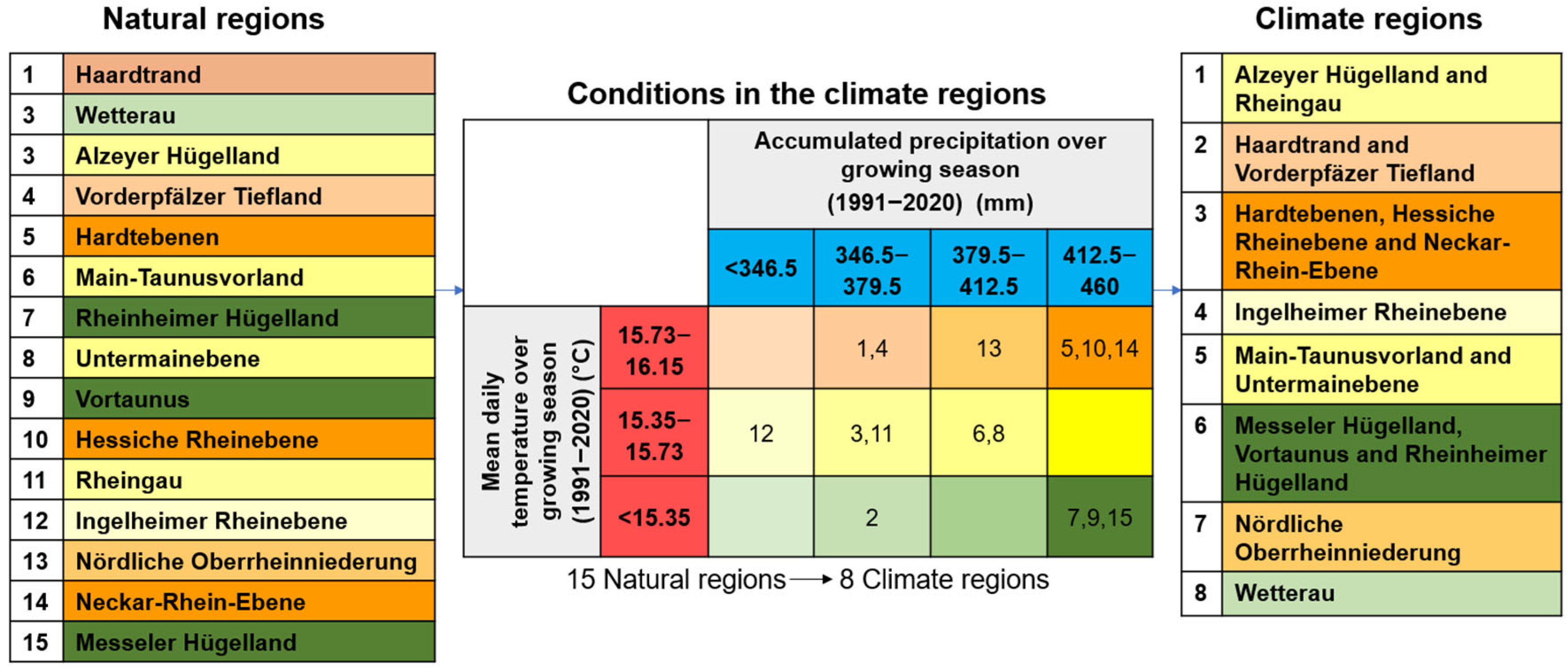
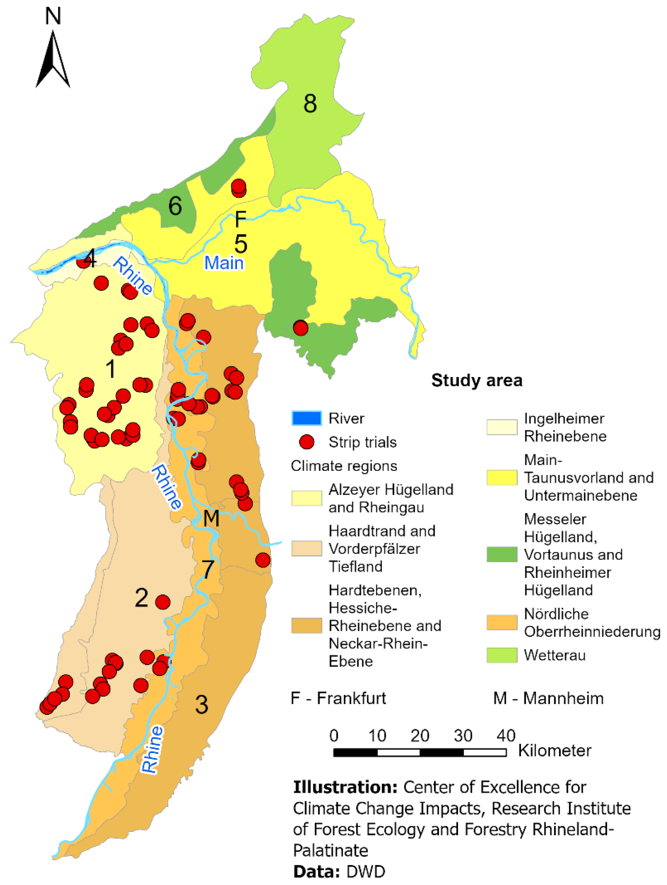
2.1. Geographical Framework

Data were collected in the areas surrounding the Rhine river, including Northern Baden-Württemberg, Southeastern Rhineland-Palatinate, and Southern Hessen. The orography of the study area is influenced by distinct features, such as the slate mountains of “Taunus”, the “Pfälzerwald”, the “Saar-Nahe-Bergland”, the “Odenwald”, and the “Spessart”. Additionally, extensive valley and basin landscapes contribute to highly heterogeneous climatic conditions in the region [11]. Dominant soils in the study area, according to the World Reference Base for Soil Resources (WRB) [12], are Cambisols, which cover 23.9% of the area and have been derived from sandy terrace deposits. Luvisols cover 14.4% of the area and usually occur in fertile loess deposits. They form the most important arable soils along the Rhine [13]. In the south, Fluvisols (14.0%) are found in the alluvial sandy loamy deposits, where agriculture is only marginal. Analogously, Fluvisols or Gleysols occupy an area of 11.3% in particularly clay-rich sediment floodplains, which often record periodic waterlogging. In the Hessian part of the study area south of the Main River, sugar beet is mainly grown on Cambisols derived from clayey sands. Occasional Luvisols, developed on clay loams and clay silts, are also present, particularly in the foothills of the Odenwald.
The study area of the SONAR (Sortenwahl für Nachhaltigkeit und Resilienz) project was divided into 15 different natural regions [14]. Natural regions are areas with distinctive features defined by their soil types, climatic regime, hydrologic regime, and type of vegetation. Natural regions capture the intrinsic ecological and physical characteristics of an area, which permits finer detail in analyzing the impacts of climate. The natural regions referenced in this study are designated as presented in Figure 1, with each region chosen due to its distinct environmental characteristics within the Rhine valley area.
The 15 natural regions in the study area were grouped into 8 climate regions based on mean daily temperature and accumulated precipitation over the growing season for the climate period 1991–2020 using the HYRAS dataset from the German Weather Service (DWD). HYRAS is a raster dataset of various hydrometeorological quantities created for Germany and the adjacent river basins and is based on observational data from ground-based weather stations. It is often used for climate and hydrological research on precipitation patterns, temperature variations, and related climatic impacts [15]. This dataset contains data from 1951–2020. The temperature data are available on a grid of 5 km × 5 km; the precipitation data are on a grid of 1 km × 1 km. Mean daily temperature in the growing season from 1991–2020 varies from 15 °C in the “Rheinheimer-Hügelland” in the north to 16.1 °C in the “Vorderpfälzer Tiefland” in the southwest of the considered region. Accumulated precipitation over the growing season from 1991–2020 varies from 342 mm in the “Ingelheimer Rheinebene” in the northwest to 460 mm in the “Hardtebene” in the southeast. Based on these values, the data are grouped into three (temperature) and four (precipitation) categories (see Figure 1, center).
The combination of these categories yielded a matrix with 12 possible climate regions. Only eight different climate regions were realized from the 15 natural regions studied herein. In these eight climate regions, trials were conducted only in seven climate regions from 2020 to 2023 (Figure 2). The numbers of sugar beet sampling locations were not evenly distributed across climate regions (see Figure 2). The field in each trial location is divided into multiple long strips laid out side-by-side. Each strip is replicated five times with different varieties of sugar beet as treatment. At these trial locations, three sticky traps were placed at the edge of the whole field instead of each strip to capture cicadas. These traps are explained in detail in Section 2.2.
The projected changes within the climate regions are assessed by three different scenarios (RCP2.6, RCP4.5, and RCP8.5) of a regional multi-model ensemble. These scenarios, known as Representative Concentration Pathways (RCP), are greenhouse gas emission trajectories formally adopted by the Intergovernmental Panel on Climate Change (IPCC). RCP2.6 is a low-emission scenario where the emissions are controlled and the temperature rise is only moderate over these years. RCP4.5 is a moderate-emission scenario. RCP8.5 is a high-emission scenario that has a steep increase in temperature, thus showing severe warming if high emissions continue [16]. Figure 3 shows that under RCP4.5 and RCP8.5, temperatures across the climate regions are expected to steadily rise until 2100. However, the rate and variability in the change of temperature are different. The mean temperature in the RCP8.5 scenario across all climate regions in the study area is projected to increase by about 2 °C by 2100 (Figure 3).
Unlike mean daily temperature, there is no clear trend in rainfall accumulated over the growing season in the future (Figure 4). Precipitation in the late 21st century shows a slight downward trend in most climate regions, especially under RCP8.5. There are regional differences in the amount of precipitation accumulated over the growing season, with some areas like “Nördliche Oberrheinniederung”, “Ingelheimer Rheinebene”, and “Wetterau” experiencing low rainfall.

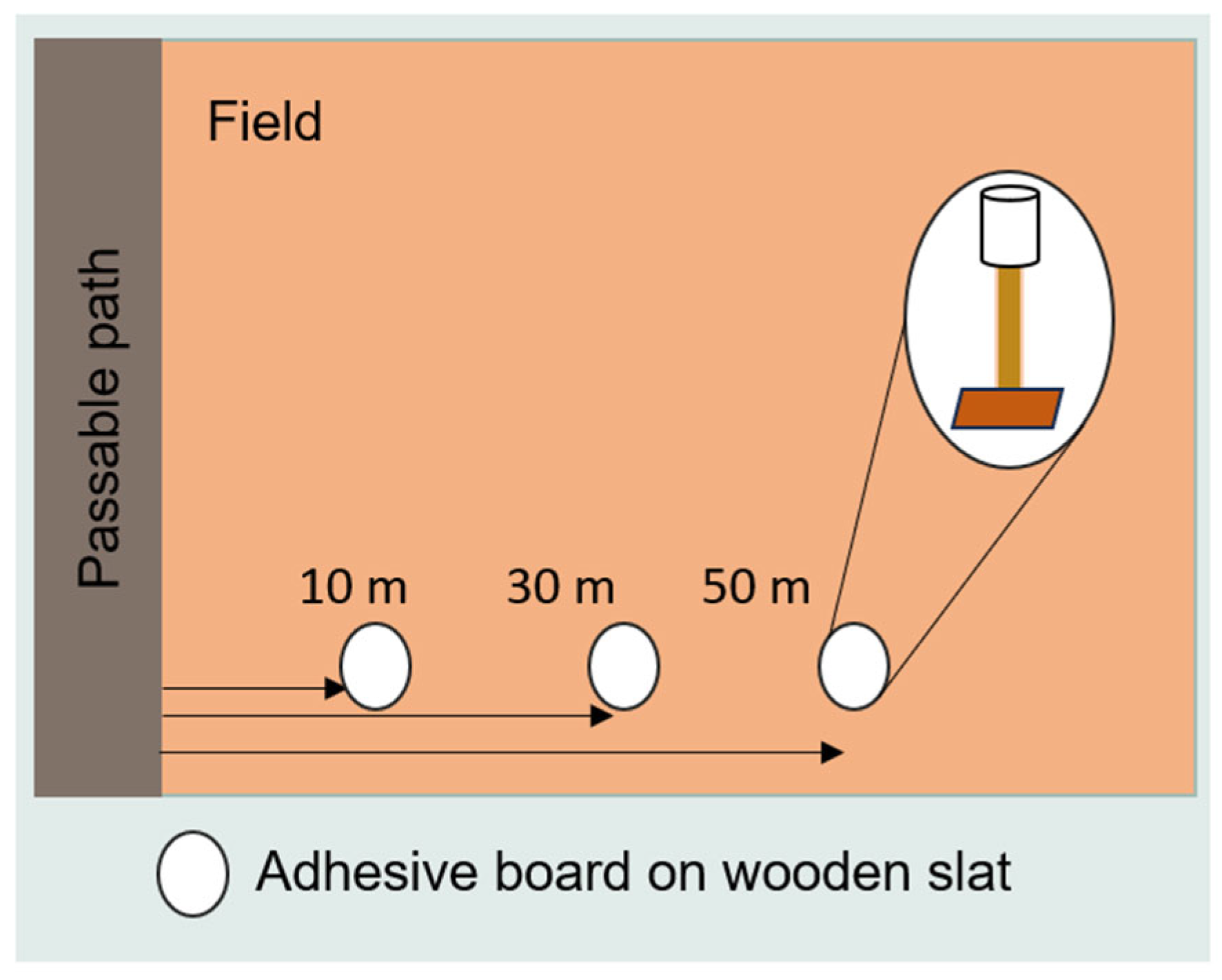
2.2. Data Collection (Cicada Field Samples)

The cicada data were collected by the Association of Hessian-Palatinate Sugar Beet Growers e.V. in two campaigns, SONAR (2022–2023) and NIKIZ (2020–2022), at 12 trial locations in 2020, at 16 trial locations in 2021, at 30 trial locations in 2022, and at 19 trial locations in 2023. In the last week of April, three sticky traps were set up at each trial location. The sticky traps were not set up separately for each strip. Instead, they were placed at the edge of whole field. The sticky traps were attached just above the height of the crop at all times. These sticky traps were attached to a wooden slat on a nail at a distance of 10 m, 30 m, and 50 m from the edge of the field as shown in Figure 5. The sticky traps were checked twice a week until cicada were first found at the respective location. After the start of the flight, the sticky traps were replaced once a week and cicada were counted in the laboratory. While sticky traps captured a variety of non-target insects, only specimens of Pentastiridius leporinus were counted and sexed based on morphological characteristics. Furthermore, SONAR includes solely sugar beet fields, whereas few NIKIZ areas in 2020 and 2021 are winter wheat fields. Our analysis is based on cicadas caught across all three traps, which are placed at each trial location. The data were checked for inaccuracies. We were unable to authenticate the accurate coordinates of two locations in the NIKIZ data for 2020. In these cases, we utilized the coordinates of the nearest city, town, or village center.

2.3. Data Preparation

For the analysis of cicada abundance, we used climate data from different time spans and different resolutions, as illustrated in Table 1. The data of climate regions were combined with cicada count data by a spatial join in ArcGIS Pro [17] where the features in the join features were matched if a target feature’s center falls within them. The joined climate region and cicada data were then merged with temperature and precipitation shapefiles using natural regions as common spatial identifier. Mean daily temperature and cumulative precipitation were obtained for the years 2020–2023, where the cicadas were counted. Projection data from Global and Regional climate model combinations were shown in Table 2. The projection data received were already bias-adjusted. They provide daily minimum, maximum, and mean air temperature at 2 m of height and daily precipitation.

2.4. Statistical Models

Generalized Linear Mixed Models (GLMM) were used in the analysis. GLMMs are an extension of generalized linear models (GLMs). They include both fixed effects (predictors with constant influence across observations) and random effects (predicted effects vary by grouping factor, like location or time) [18]. GLMs and GLMMs often deal with response variables that do not naturally align with a simple linear relationship, such as count data, binary data, or proportions. The frequency distribution of our cicada count data is right-skewed. There is a substantial proportion of zeros in the data because cicadas do not fly in the very beginning of the growing season when sticky traps are set up. This proportion changes over time with extreme counts on some days. We used a GLMM with a negative binomial distribution (log–link function) for analyzing our count data with overdispersion. Overdispersion occurs when the variance of the response variable is larger than expected under a Poisson model. The negative binomial model accounts for this extra variability [19]. Data evaluation was done separately for male and female cicadas.

2.4.1. Model 1

A GLMM was set up with expected count of cicada in each trap interval. The outcome variable is observed reed glass-winged cicada count ( R G W C i j k l o ) , and the categorical variable climate region (c) is fixed factor. The categorical factors year y , month m , and the location l were considered random. Model 1 reads:
log E [ R G W C i j k l o ] = η i j k l o = α + c i + c y m i j k + c l i l + l o g ( δ i j k l o )
where η i j k l o is linear predictor linked to the expected value (mean; E[.]) of the observed count R G W C i j k l o using a log–link in the ith climate region, in the jth year, in the kth month, at the lth location, and oth trap interval, while α is the overall intercept, c i represents a fixed effect of the ith climate region, c y m i j k represents a random intercept for year–month combinations j k within climate region i , c l i l represents a random intercept for the lth location within climate region i , and δ i j k l o refers to the time interval in days for the ith climate region, jth year, kth month, lth location, and oth trap interval. The offset l o g ( δ i j k l o ) was used to normalize parameters in the linear predictor to a count per day, effectively adjusting for different length of time intervals when comparing counts across different periods or locations.
The observed count was assumed to be distributed as negative binomial (N.B) with mean μ i j k l o and dispersion parameter ϕ , which is the scale parameter:
R G W C i j k l o ~ N . B ( μ i j k l o , ϕ )
Both mean and dispersion parameter determine the variance of the observations. This is where residual error occurs. The data were on the original measurement scale when fitting the GLMM. An inverse log–link function, i.e., the exponential function, was used to transform the means from model scale back to the original scale. These means are assessed on a count-per-day basis. To distinguish these from the means corresponding to the observed counts, we denote these means using a tilde:
μ ~ i j k l o = e η i j k l o = e α + c i + c y m i j k + c l i l
where μ ~ i j k l is the expected count per day in the ith climate region, jth year, kth month, and lth location. Considering the random factors location, year, and month, we computed the expected mean count for the ith climate region as
μ ~ i = e α + c i + v a r ( c l i l ) / 2 + v a r ( c y m i j k ) / 2
μ ~ i = e α + c i e v a r ( c l i l ) / 2 e v a r ( c y m i j k ) / 2
These equations consider that under the assumption of normality of the random effects, the expected counts have a log–normal distribution. The “glmmTMB” package in R 4.4 [20] was used to fit the GLMM and “Emmeans” package [21] to calculate marginal mean cicada responses for each climate region. The back-transformed marginal means were termed as model means. Pairwise comparisons of expected mean cicada counts were performed using the Tukey HSD (Honestly Significant Difference) test to assess significant differences between climate regions. Means for each climate region were then plotted. The resultant estimates of the expected mean E [ R G W C i j k l o ] were compared visually with trial results for each climate region. The variance components v a r c l i l and v a r ( c y m i j k ) obtained from the GLMM focus on the multiplicative effect (how much higher or lower counts are relative to the mean). Since the variances are obtained on the log–link scale, they are dimensionless.
The Wilcoxon signed-rank test, a non-parametric alternative to the paired two-sample t-test, was conducted before this analysis to compare male and female cicada samples from the same traps in the climate regions. This test considers the dependent nature of the data, as each trap simultaneously records both male and female individuals. The analysis was performed to test whether male and female cicadas were statistically different in the various climate regions [22].
In this analysis, months, years, and locations were considered as random effects to account for repeated measures, since they are hierarchically nested within climatic regions. Climatic region was set as a fixed effect as it is related directly to our research question.

2.4.2. Model 2

Model 2 was set up to test the quantitative relationships between climatic variables and cicada counts. In ecology, associations between climate factors and species responses tend to be nonlinear. Adding quadratic terms provides a model with the flexibility to describe curvilinear relationships. To investigate how temperature and precipitation influence the cicada populations, we replaced the categorical fixed effect climate region variable from Model 1 with linear and quadratic terms of temperature and precipitation. There was no significant interaction found between temperature and precipitation. Model 2 reads:
l o g ( E [ R G W C i j k l o ] ) = α + β M t M t i j k l + β M t 2 M t i j k l 2 + β M p M p i j k l + β M p 2 M p i j k l 2 +   c y m i j k + c l i l + l o g ( δ i j k l o )
where l o g ( E [ R G W C i j k l o ] ) represents the logarithm of the expected count of cicada in the ith climate region in the jth year, in the kth month, at lth location, and oth trap interval with covariates from climate region, while β M t is the regression coefficient for mean temperature, M t i j k l represents the temperature in the ith climate region, in the jth year, kth month, and at lth location; β M p is the regression coefficient for precipitation, and M p i j k l represents the precipitation in the ith climate region, in the jth year, kth month, and at lth location, while α is the intercept term, c y m i j k represents a random nesting effect of climate region i , year j , and month k , and c l i l represents the random nested effect of climate region i and location l , and l o g ( δ i j k l o ) represents an offset that is used to normalize parameters of the linear predictor to counts per day.
First, we analyzed Model 2 with long-term averages of temperature and precipitation over 30 years (1991–2020) in the growing season (April–October) for each climate region as input data. Then, we analyzed with daily mean temperature and daily precipitation (2020–2023) in the growing season (April–October) for each climate region as input data. To ensure consistency and comparability, before the analysis, temperature and precipitation were separately standardized using dataset-specific means (18.20 °C, 2.09 mm) and standard deviations (4.02 °C, 4.25 mm) to ensure consistency and comparability. This transformation ensures that both variables have a mean of zero and are scaled to unit variance relative to their observed variability. Parameter estimates were obtained for the standardized predictors. The standardized predictors were named as “Scaled mean temperature” and “Scaled precipitation” in the analysis. With both long-term averages and daily weather data, we calculated marginal R2 ( R m 2 ) and conditional R2 ( R c 2 ) using the “MuMIn” R package. The marginal R2 shows the proportion of variance explained by fixed effects only, while the conditional R2 includes both fixed and random effects and, thus, is a measure of total variance explained.
We calculated mean expected cicada count and 95% confidence intervals using “Emmeans” package. This was done by generating a sequence of 100 equally spaced values between the minimum and maximum scaled temperature and precipitation values from the input daily and the long-term climate data, respectively. The scaled input data values were then back-transformed to their original scale using the means and standard deviations from their respective datasets. The observed data points were normalized to count per day by dividing the cicada counts ( R G W C i j k l o ) by the observation day interval ( δ i j k l o ). Then, we averaged the counts per day and grouped them by temperature and precipitation values, respectively, so that we got mean cicada count per day in accordance with the observed data. The observed data and predicted response curves were then plotted against the range of predictor variables for the whole study area, not specifically for any climate region.

2.4.3. Model Validation
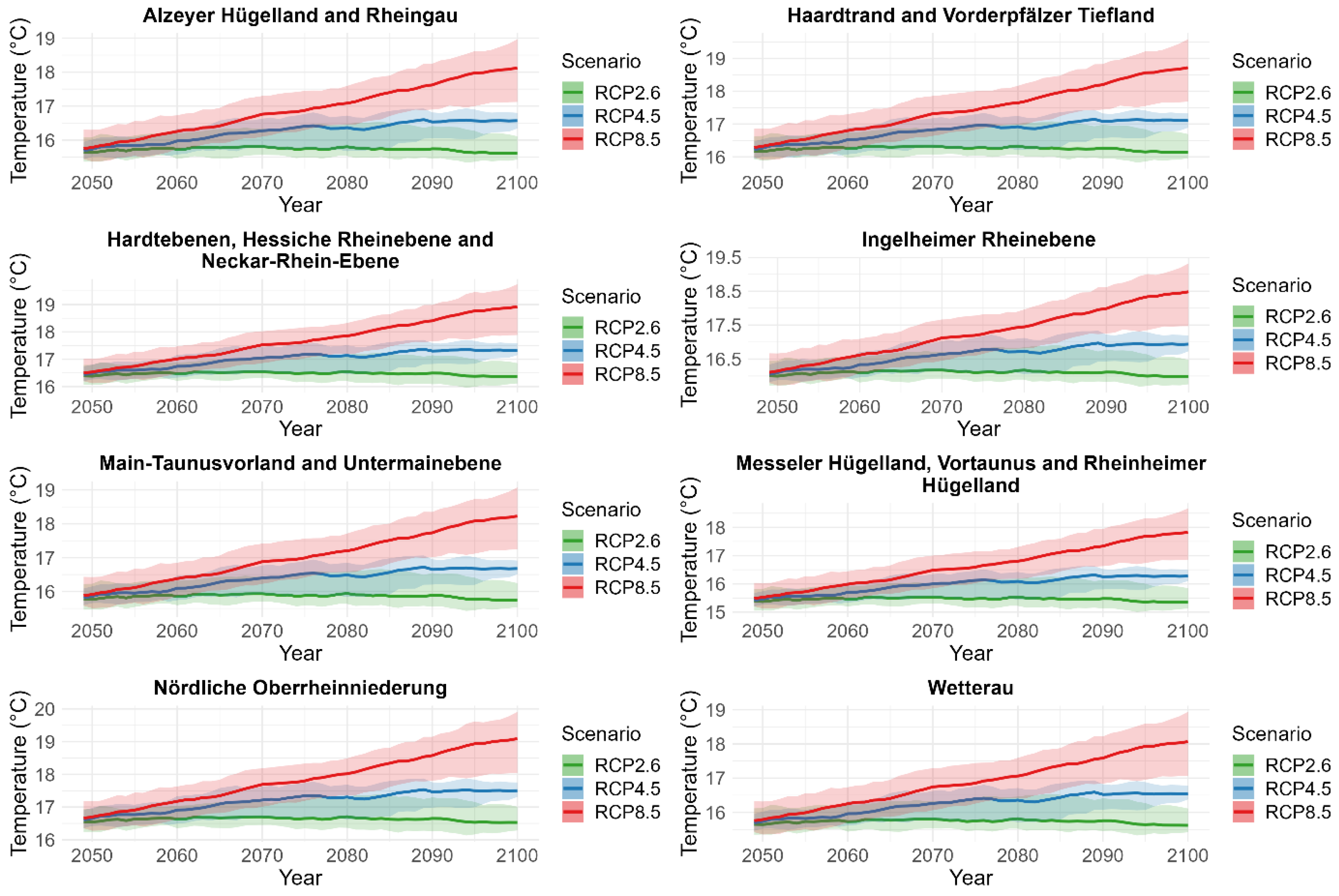
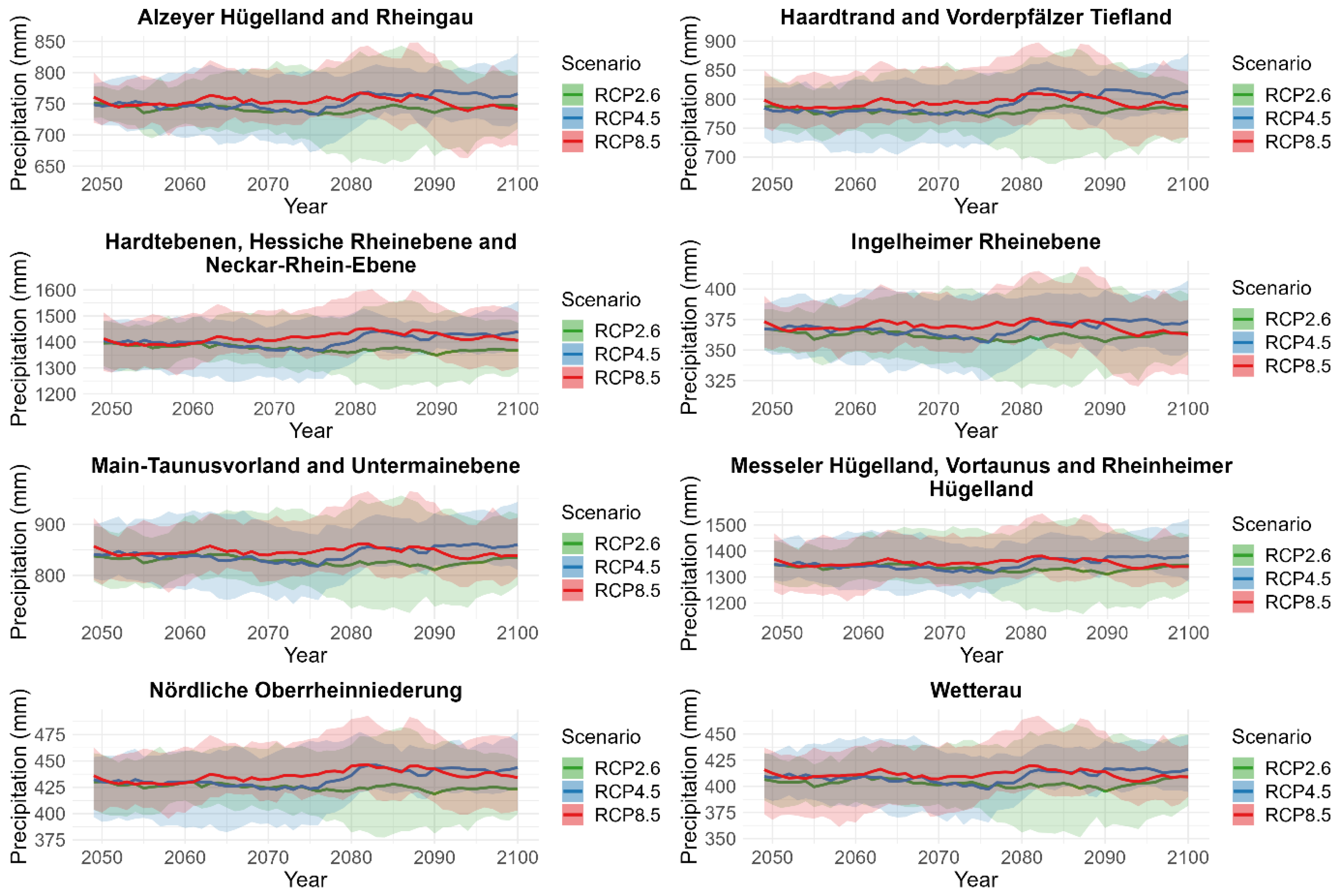
Model validation was done using the “DHARMa” package (Residual Diagnostics for Hierarchical Models) in R to assess the model fit and potential issues [23]. This R package generates simulated residuals to check some of the important assumptions of the model, such as dispersion, residual randomness, and distribution. “DHARMa” performs dispersion test for overdispersion or underdispersion of the residuals, a Kolmogorov–Smirnov test to assess the deviations of the residual distribution from the expected distribution, and an outlier test to detect significant outliers.

2.4.4. Projections

Model 2 was used to project future male and female cicada abundance. Mean daily temperature and precipitation data from the three climate projection scenarios under regional multi-model ensemble (Table 2) were used for the cicada projection. We used daily weather data in Model 2, but monthly climate projection data to predict conditional means. Only climate region-specific projections were employed so that the predictions reflect the average behavior across all locations within a particular region rather than predictions for specific locations. From the predicted values and standard errors, the 95% confidence intervals were calculated based on a negative binomial distribution.
Model predictions obtained were mean trends and were not easily related to actual field observations. Observed cicada counts reached high levels during specific conditions (e.g., up to 300 counts per week or 50–60 counts per day in traps of some locations). However, the raw model predictions were considerably lower in counts and did not represent this biological reality. Scaling adjusted the mean predictions to align well with observed peaks. Predictions were adjusted using region-specific scaling factors derived from the ratio of the lowest value of the 95th percentile of maximum daily cicada counts to the mean daily counts for each region from the observed data. The scaled predictions for individual regions were aggregated across all regions for each year and RCP scenario to represent the entire study area. This adjustment is intended only for demonstration purposes to show the maximum daily counts that can be expected in the future. This adjustment did not interfere with the model fitting process or violate statistical assumptions since it is only applied to predictions after the modeling.

3. Results

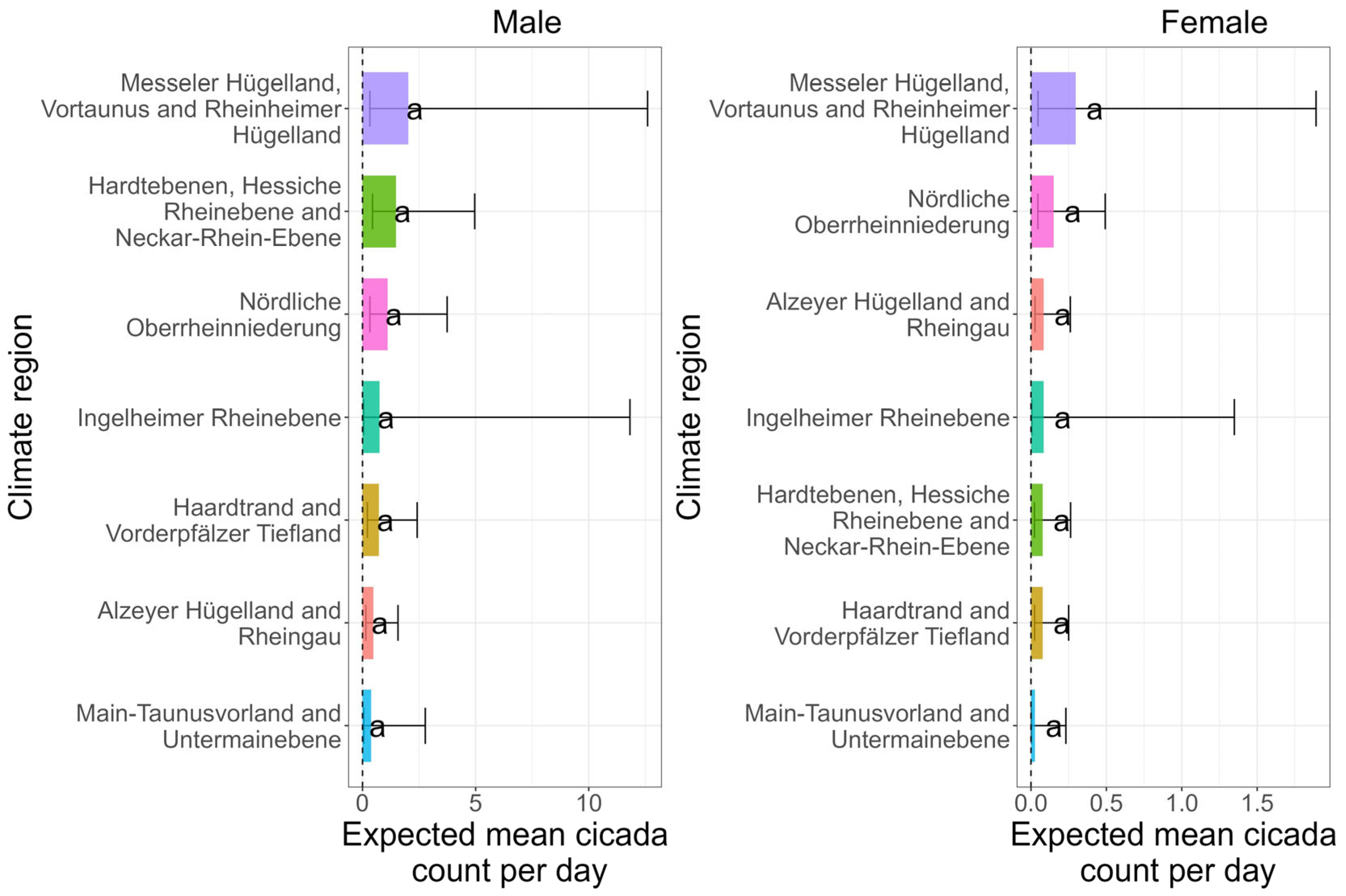
3.1. Does Cicada Abundance Differ Between Climate Regions?

Figure 6 shows expected mean cicada counts per day across the seven climate regions, based on Model 1. For both male and female cicadas, there were no significant differences between climate regions. The number of male captures was higher than the female captures. Based on the Wilcoxon signed-rank test, male and female cicada captures are statistically different at p-value < 0.001.
Table 3 shows the variance components of Model 1 on the log–link scale. The variance among the climate regions was accounted for by a random effect. However, there was no variance in cicada counts between climate regions left if the other factors temperature and precipitation were also accounted for. The biggest variance contribution originates from the nested year and month effect in the climate region followed by the effect of location.
Table 4 compares Model 1 means with observed sample means. Model 1 means were back-transformed from the log–link scale. The model means for male cicadas in some regions is up to 70% higher and, in others, up to 72% lower than the observed counts. For female cicadas, the model means are up to 100% higher in some regions and, in others, up to 67% lower than observed counts. In only two-to-three regions, respectively, the model means correspond well to the observed results.

3.2. To What Extent Do Mean Temperature and Precipitation of Climate Regions Influence Cicada Populations?

3.2.1. Impact of Long-Term Averages (1991–2020) on Cicadas

Cicada abundance did not significantly vary between climatic regions. Therefore, we investigated whether the 30-year means of temperature and precipitation influenced cicada abundance separately. Table 5 shows the parameter estimates of Model 2, when long-term averages of temperature and precipitation over a 30-year period (1991–2020) during growing season (April–October) for each climate region were used as explanatory variables. The estimates presented in Table 5 are on the log–link scale and were derived for the scaled predictors. Table 5 shows that neither mean temperature nor precipitation had a significant influence on cicadas. Similar to Model 1, the major proportion of variance in Model 2 originates from the year and month ( c y m ) nesting effect.

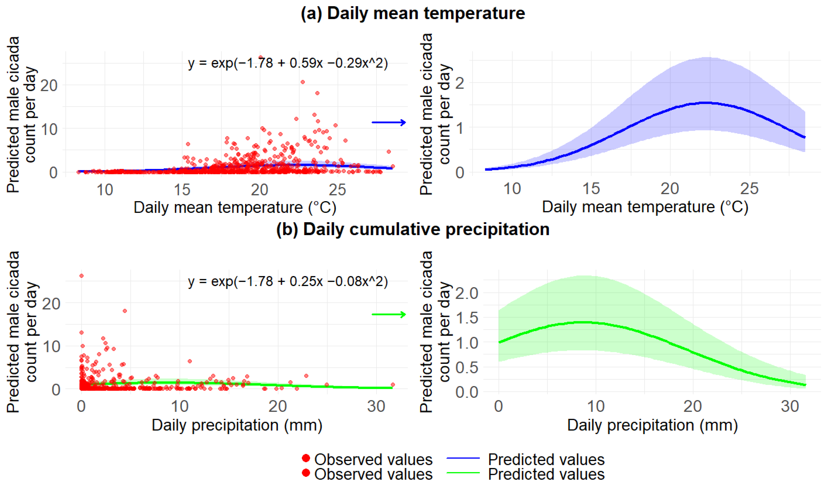
3.2.2. Impact of Daily Weather on Male Cicadas During 2020–2023

Table 6 shows the parameter estimates and variance components of Model 2 when the daily weather data (2020–2023) were used. Daily mean temperature and daily accumulated precipitation had a significant non-linear effect on male cicadas. The variance on the log–link scale for climate region, year, and month c y m nesting effect is greater than that for climate region and location ( c l ) effect. The variability across months and years within climate regions is more pronounced compared to the variability between specific locations within a region.
Figure 7 shows the influence of daily mean temperature and daily precipitation on male cicada flight activity through quadratic response curves. The male cicadas’ flight activity was optimum around a 22 °C daily mean temperature in the growing season. Towards lower and higher temperatures, male cicada counts decrease.
The influence of precipitation on male cicada counts also shows an optimum shape. The optimum is at about 8 mm daily precipitation. Male cicada flight activity was high when there was zero to moderate rainfall. It decreased to zero as precipitation increased.

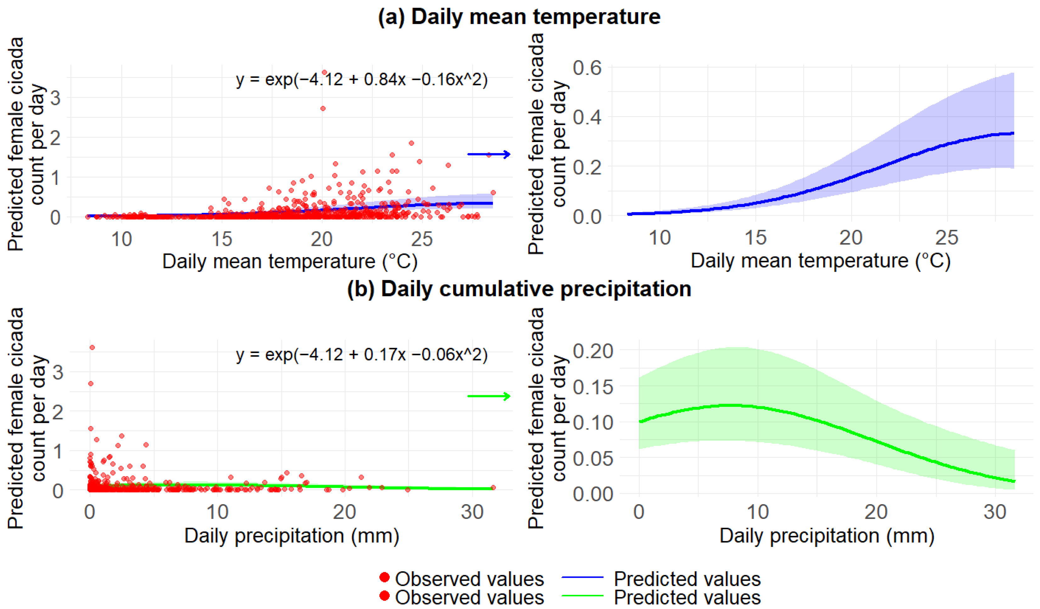
3.2.3. Impact of Daily Weather on Female Cicadas During 2020–2023

Daily mean temperature and daily precipitation also exhibited a significant non-linear effect on female cicadas from 2020–2023 (Table 7). The variance for year and month ( c y m = 3.60) nesting effect within climate regions is more pronounced than the location ( c l = 0.65) effect.
Female cicada flight activity peaked around 28 °C (Figure 8). Their activity is low when it is cold. Female cicada flight activity was high from zero-to-moderate rainfall. It was optimum when daily precipitation was around 8 mm/day. Female numbers declined when it rained a lot.

3.2.4. Comparison of Long-Term Average and Daily Predictor Variables

Table 8 compares R2 values of Model 2 when using daily weather data (2020–2023) and long-term climate averages (1991–2020). Marginal R-squared ( R m 2 ) considers only fixed effect variances, whereas conditional R-squared ( R c 2 ) considers both fixed effects and random effect variances. The marginal R2 is considerably higher for daily data, with 7.1% for the male and 12.2% for the female cicada, in comparison with long-term averages data at 2.5% for males and 1% for female cicadas. With daily data, temperature and precipitation could capture the responses of cicadas better. Long-term averages diluted the effects of short-term weather events that are critical for activity, reducing their explanatory relevance. Because of the substantially higher marginal R2, we restricted the following analysis to using only daily weather data.

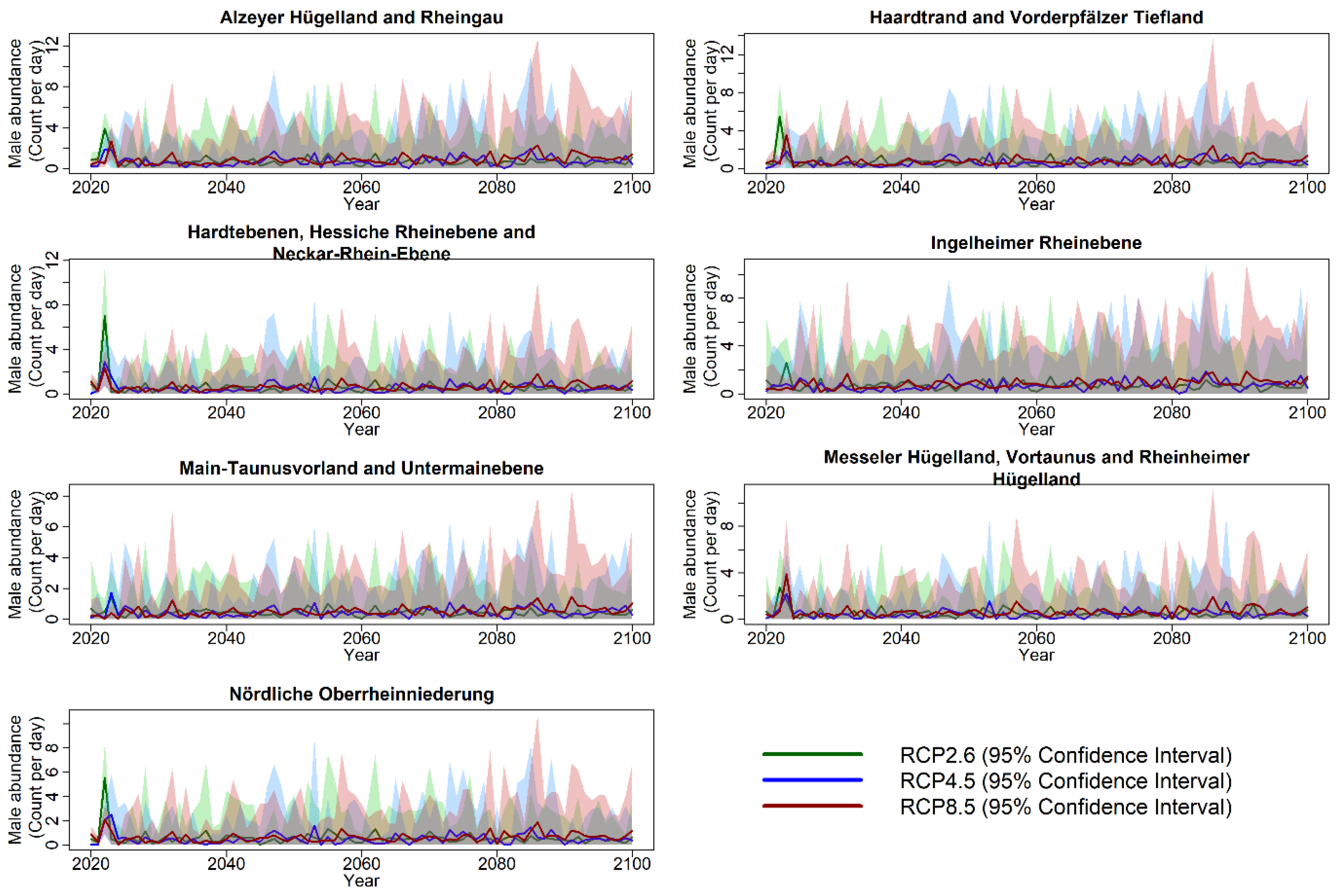
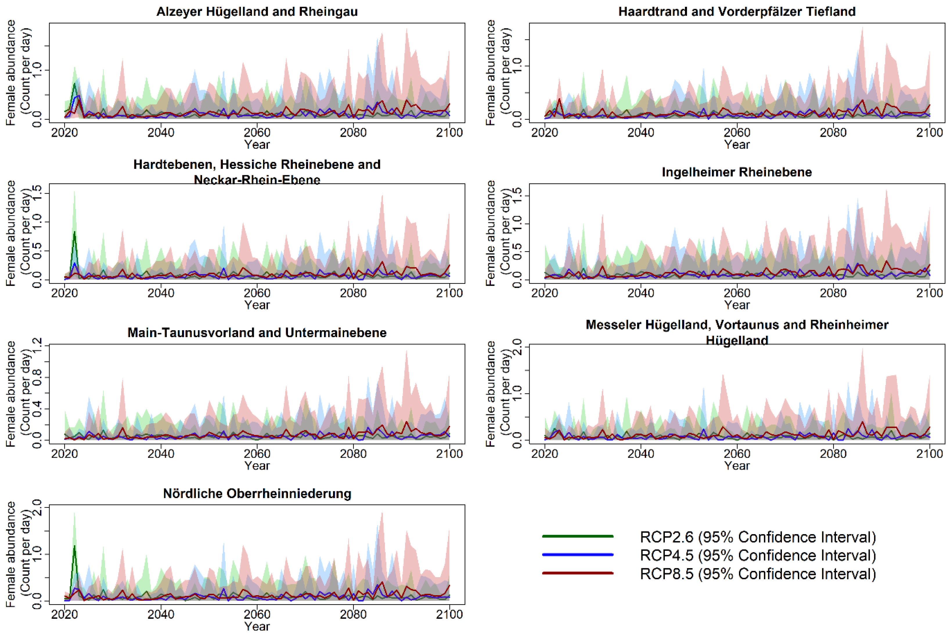
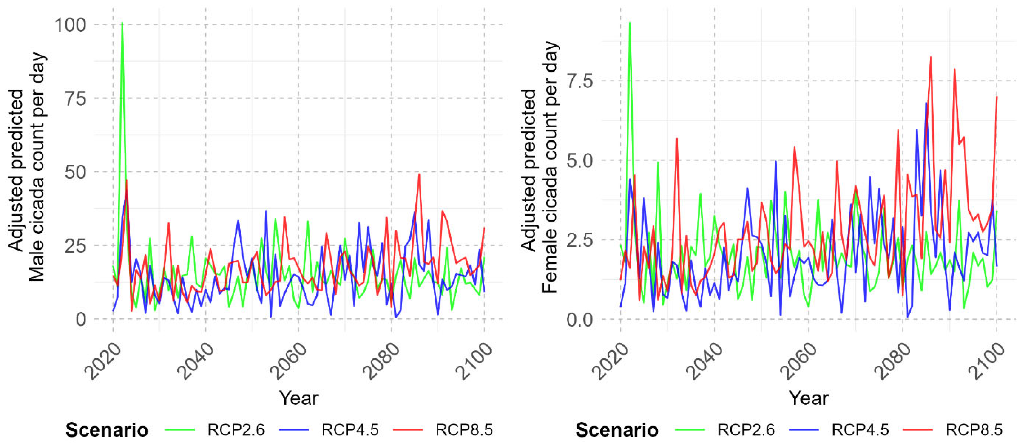
3.3. Projection of Cicada Abundance Using Climate Projections

Multi-model ensemble simulations (Table 2) of future monthly temperature and precipitation were used to predict the cicada abundance until 2100. Due to the model offset, the predictions obtained were daily counts. In Figure 9 and Figure 10, cicada predictions were visualized for each climate region, along with the 95% confidence intervals. Climate change, particularly under the worst-case scenario (RCP8.5), will produce increased cicada counts in future. This was observed by examining the upper limit of the 95% confidence interval (shaded in red), which represents the maximum likely predicted daily abundance of male cicadas. Figure 9 shows the mean count of male cicadas reaching a peak of 8–12 counts per day in certain regions under the RCP8.5 scenario. By the end of the century, under RCP2.6, male cicada counts were projected to be four-to-five cicadas per day, which is lower by 60–70% compared to the RCP8.5 scenario.
Figure 10 shows that the female cicada counts by the end of the 21st century in RCP8.5 scenario are projected to reach one-to-two counts/day, which is 10 times higher than today’s number. This increase is similar to that of male cicadas. However, the count of female cicadas per day is 70–80% lower than that of males. The low-emission scenario RCP2.6 shows a decrease in female cicada count per day up to 70% when compared to RCP8.5.
Since the above predictions are mean counts averaged across the growing season and, hence, do not represent the full natural variability, we scaled the mean predictions in Figure 9 and Figure 10 to maximum values and aggregated the resulting counts across the whole study region. Figure 11 shows the rescaled daily maximum male and female cicada counts averaged across the growing season until 2100 for the study area under three climate scenarios. For male cicadas, the projections under RCP2.6 can reach up to 100 counts per day during 2020–2030. While these unusually high values represent uncertainties in the climate projections (see Section 4.2), beyond this initial period, RCP2.6 male counts stabilize, fluctuating between 0–30 counts per day for the rest of the century. In contrast, RCP4.5 shows similar moderate activity, rarely reaching 30 counts per day, while RCP8.5 resulted in elevated counts at the end of century, with the adjusted predictions reaching up to 40 counts per day.
A similar pattern emerges for female cicadas (right panel), although at a lower magnitude. Under RCP8.5, daily counts fluctuate up to five counts per day, with occasional peaks reaching seven female cicadas per day. Conversely, RCP4.5 results in moderate activity, with up to five counts per day, although this is infrequent. Finally, RCP2.6 shows subdued activity, with daily counts ranging between 0 and 3 counts per day, with rare peaks of four counts per day.

4. Discussion

4.1. Influence of Climate Regions

Our analysis using Model 1 showed that the abundance of both male and female cicadas (P. leporinus) did not vary significantly between climate regions in the Upper Rhine valley. Climate regions were defined based on the combinations of long-term average temperature and precipitation (Figure 1). Due to the lack of significant variation between climate regions, we investigated whether the individual climate factors (30-year means of daily temperature and accumulated precipitation (1991–2020) during the growing season) independently influenced cicada counts using Model 2. However, we found that neither of them was significant, implying that long-term climate averages during 1991–2020 did not strongly affect cicada abundance.
Variance components in Table 3 were presented on the log–link scale as a log–link function was used in the model. This approach is standard for GLMMs as it keeps the variance components additive on the log scale [24]. The discrepancies between the model prediction and the trial measurements in Table 4 indicate the weaknesses of the model in representing cicada counts in the climate regions. These discrepancies may originate from uncertainty in model parameters due to incomplete datasets in 2020 and 2021 and unbalanced sampling across the climate regions, as well as from environmental and biophysiological factors not considered by Model 1. Future studies should look into the effects of vegetation structure, soil, predator–prey dynamics, and pesticide use since these could influence the distribution and behavior of P. leporinus.

4.2. Influence of Temperature and Precipitation

Cicadas were more sensitive to short-term weather variations rather than long-term climatic averages. A moderate rise in daily mean temperature in the growing season of 2020–2023 increased the male cicada flight activity. This is consistent with their thermophilic nature. Conversely, high temperatures impeded cicada activity, likely due to thermal stress or the impact of convective storms and heavy rains often linked with hot days during this timeframe. High temperature had a stronger positive effect on female cicada activity compared to males, aligning with our observation that male cicada counts peaked in June, while females peaked in July. Notably, July temperatures were higher than in June during 2020, 2022, and 2023. This temporal divergent behavior between male and female activity is consistent with the established role of temperature as a primary determinant of Hemipteran phenology. Whereas the study of Moriyama and Numata (2019) is about true cicadas (Cicadidae), it shows that temperature is a basic environmental variable affecting insect ecophysiology, ranging from activity patterns to development schedules [9].
Sticky traps recorded a greater number of male cicada specimens when compared with females. The high counts of capture recorded do not necessarily represent the actual sex ratios in the field populations but may reflect differences in behavior of males and females. In certain hemipteran species, i.e., cicadas and planthoppers, males have longer or more active flight behaviors when mating seasons are on, thereby putting them at a higher chance of being caught [25]. While the general flight activity of P. leporinus has not been fully clarified, this description is reasonable in light of what has been found in comparable species, e.g., Hyalesthes obsoletus [26,27]. For instance, male insects have generally sustained flights, seeking mates and defending territories, thereby increasing chances of capture in the course of these activities. The unusual peak in 2022 for predictions under RCP2.6 in Figure 9, Figure 10 and Figure 11 was likely due to short-term fluctuations in temperature and precipitation in the climate model “MIROC-MIROC5_r1i1p1_CLMcom-CCLM4-8-17”, which may have introduced temporary anomalies in the projected cicada counts. In particular, during the growing season, the median monthly temperatures in different climate regions increased from about 16–17 °C in 2021 to almost 19–20 °C in 2022, while the cumulative monthly rainfall declined from 80–100 mm to about 50–70 mm. This drastic shift towards warmer and drier climatic conditions is in agreement with the expected climatic optimum for cicada abundances, thus explaining the spike in the model-predicted abundances in 2022, as per the RCP2.6 scenario.
Under RCP8.5, a rise in mean counts for both male (8–14 counts/day) and female cicadas (1–2 counts/day) was observed in response to rising temperatures across climate regions. Conversely, fluctuations in mean precipitation within the climate regions introduce uncertainty. In contrast to RCP8.5, the predicted counts in RCP2.6 were 60–70% lower. Figure 9 and Figure 10 show that the impact of climate change on cicadas is not uniform and varied between different climate regions. This may be due to differences in the number of trial location samples used in the model. For example, regions such as “Alzeyer Hügelland and Rheingau” with more than 10 trial locations showed more pronounced counts compared to the regions with fewer samples, such as “Main-Taunusvorland and Untermainebene”, with only one trial location. The unbalanced sampling may have affected the regional differences observed in the predictions in Figure 9 and Figure 10. This points to the necessity of balanced data to achieve robust regional comparisons in future. This points to the necessity of balanced data to achieve robust regional comparisons in future. To check if this imbalance compromised the predictive performance, we compared the male model performance using Root Mean Squared Error (RMSE) in well-sampled, poorly sampled, and combined datasets. While poorly sampled regions had higher RMSE values (13.6 counts/day), their inclusion in the combined model did not reduce the overall predictive accuracy substantially, as the combined model RMSE (10.6 counts/day) was close to that for the well-sampled group (10.4 counts/day). Albeit sample representation was low in certain regions, overall model predictions were very robust. However, predictions in the poorly sampled climate regions, such as “Ingelheimer Rheinebene”, “Main-Taunusvorland and Untermainebene”, and “Messeler Hügelland, Vortaunus, and Rheinheimer Hügelland” (Figure 9 and Figure 10) should be viewed with caution.

4.3. Limitations of Model 2

Figure 12 shows “DHARMa” diagnostic plots for Model 2 for both male and female cicadas when daily weather was used as predictors [23]. The Kolmogorov–Smirnov (KS) test from Figure 12 reveals significant deviations (p < 0.001) from the expected residual distribution for both male and female cicada models. This is further supported by the observed patterns in the quantile–quantile plot (QQ plot), which show discrepancies between observed and expected residual distributions, particularly at the tails. This is a sign that the model may be missing to capture the full variability of the underlying data. There is also a significant presence of outliers (p < 0.01) in our data that the model finds challenging to accommodate. In our case, these are high cicada counts. Therefore, they were not removed.
Our model performed well for lower counts but had some difficulties in representing the extreme values. The obvious nonrandom pattern in the residuals suggests that the quadratic terms do not capture all of the nuances of the relationship, or that additional predictors such as vegetation structure, land use, or local pesticide application might have affected the counts. The female version of the model handles the variability better than its male counterpart. Residual patterns and some significant outliers (p < 0.01) indicate that further refinements may be necessary. To explore this, we used a generalized additive model with penalized splines for the temperature and precipitation variables. However, the predictive performance of this spline-based model was poorer than that of the quadratic model, with a higher RMSE (15.6 and 2.2 counts/day compared to 10.6 and 1.6 counts/day for male and female models). The quadratic model was, therefore, selected as the better, more parsimonious option. However, future studies employing an expanded dataset—specifically one containing ecological or management variables—could benefit from the use of flexible modeling approaches, such as hierarchical splines, thus increasing predictive accuracy [28].

4.4. Implications for Crop Diseases

Peak activity for male cicadas occurred at approximately 22 °C, while for female cicadas, it occurred at 28 °C. However, excess precipitation above 8 mm reduced activity for both male and female cicadas to zero. From a plant protection perspective, there are implications of our findings: increased temperatures lead to higher cicada activities in sugar beet fields and may allow the pest to thrive, multiply, and spread into adjacent farms and infest them, leading to crop losses [29,30]. Heavy rainfall could temporarily act as a natural control mechanism, which might reduce the spread as waterlogged conditions can adversely impact flight behavior and also nymphal survival [31]. This fluctuating relationship between temperature, precipitation, and the populations of cicadas shows that more dynamic and adaptive approaches will be required by the farmers to manage the consequences.
The increasing prevalence of the reed glass-winged cicada, Pentastiridius leporinus, and its close relative glass-winged cicada, Hyalesthes obsoletus, as vectors of plant pathogens “Candidatus Phytoplasma solani” and “Candidatus Arsenophonus phytopathogenicus for diseases in sugar beet and potato crops presents a serious concern for agricultural health and food security [5]. Reed glass-winged cicadas are reaching high population densities in sugar beet fields and potato fields [32,33]. The lack of permitted pesticides for cicadas creates a precarious situation for farmers, who may be ill-equipped to manage the risks posed by these vectors effectively [4]. Our results suggest that climatic conditions, in particular warmer and moderately dry growing seasons, are conducive to high cicada densities. This will mean that the disease transmission risk may be increased due to high cicada densities during such climatically favorable windows, which are likely to increase in frequency under climate change. The erratic nature of pathogen transmission, influenced by environmental factors and the presence of reservoir plants, complicates efforts to establish reliable control measures [34,35].
At the moment, there is no established risk or action threshold for the reed glass-winged cicada. For the sake of comparison, the risk threshold for planthopper Psammotettix alienus is 30 counts per week in yellow sticky traps in France [36]. This leafhopper is a distant relative of the P. leporinus and is responsible for transmitting the Wheat dwarf disease. This disease is also relevant in Germany. These leafhoppers are responsible for sucking phloem sap from the vegetative sections of wheat with their mouthparts, thereby transmitting the wheat dwarf virus. Our model outputs from Figure 11, which projected expected daily counts of P. leporinus under different climatic scenarios, could provide a basis for developing such risk thresholds.
The economic ramifications of sugar beet are profound, with reports indicating yield losses of up to 30% due to SBR, characterized by yellowing leaves, stunted growth, and diminished root development [5,37]. Farmer statistics in the region Hesse show a decrease of 17.43% in polarized sugar content from 2020 to 2023, from 17.7 to 14.6%. In the Palatinate region, a decrease of 17.4% was observed from 17.5 to 14.7%. In the Rhine-Hesse region, a higher decrease of 20.2% from 18.9 to 14.3% was observed. When averaged across the three regions, the overall decrease of polarized sugar content in the study area during 2020–2023 was approximately 18.4%. Notably, our model’s forecasted cicada peak density is in 2022, during this period of sugar downturn. While we do not claim direct causation, the time coincidence suggests that years of high vector activity, as forecast by our model, can have an effect on crop-quality loss. This reinforces the model’s applicability for pest risk forecasting to select suitable agricultural management measures.
Lang et al. (2025) extrapolated P. leporinus propagation based on data from Pfitzer et al. (2022) [4,38]. According to them, maximum rates of reproduction are typically reached within 3–4 years following the species’ establishment within a new area. The reproductive timeline outlined by Lang et al. (2025) could be further altered by the rise in temperatures and changes in the pattern of rainfall [38]. High mean daily temperatures, as mentioned in our study, will likely speed up the female developmental rate, which will lead to peak cicada population within a time frame less than the 3–4 years estimated by Lang et al. (2025), perhaps within 2–3 years. Such an alteration will significantly raise the chances of more frequent and intense cicada outbreaks with important implications for sugar beet and other vegetable crop yields (potatoes, carrots, beetroots, etc.) [38]. Lang et al. (2025)’s 6-year cicada population projection shows a population of more than 67 million individuals, indicating the potential for rapid outbreaks [38]. These assumptions emphasize the need for early identification within the first 3–4 years to curb the growth of P. leporinus before it reaches maximum reproductive capacity.
There is currently no general solution for the cicada problem. Because the cicadas need their plants to overwinter in the field, a promising practical solution is to leave fields fallow over winter [33]. This entails some economic loss and, more importantly, fallowing must be conducted in concerted action by farmers over a few square kilometers because the cicadas are very mobile when they fly out in spring. This approach is currently being tested in some federal states. Our current modeling results focused on weather variables of the growing season. They highlight the strong association of precipitation, temperature, and cicada populations. However, it is likely that weather conditions of the previous winter can also influence their population dynamics. This question will be evaluated in a follow-up study in which we consider the lagged effects of extreme weather conditions experienced during the overwintering stage (winter and spring) on cicada populations in the following growing season.
Further, research is underway to develop SBR-tolerant cultivars, which is a positive development. In this context, our modeling of climate-driven fluctuations in cicada abundance offers a valuable tool for anticipating high-risk years for vector pressure. Identifying climatic windows when cicada populations are likely to surge, such as the unusually wet 2021 growing season, followed by the warm and dry 2022 growing season, can inform timely disease monitoring and management strategies. This is particularly relevant for integrated pest and disease control in sugar beet systems under climate change. While phytoplasmas are the primary concern, cicadas could also facilitate the entry of other pathogens through feeding wounds [38]. SBR infection weakens sugar beets, making it easier for opportunistic fungi to infect them. A prominent example of a secondary fungus in SBR-infected sugar beets is Macrophomina phaseolina [39]. Moderate daily precipitation (up to 8 mm), as discussed in our study, could potentially supply critical moisture for both cicadas and opportunistic fungi like Macrophomina phaseolina to develop and prosper. This shared climatic suitability could also enhance disease pressure on vulnerable agricultural crops. The implications of these diseases extend beyond individual crops to regional economic well-being. The interconnectedness of agricultural systems means that the decline of sugar beet and potato yields could disrupt supply chains, affecting not only farmers but also consumers and related industries [40,41]. As climate change continues to alter environmental conditions in the agroecosystems, as mentioned in our study, the potential for increased vector populations and pathogen transmission becomes even more pronounced, necessitating targeted measures and innovative solutions [42,43].

4.5. Limitations and Future Directions

This study focused particularly on the effects of two key abiotic climate drivers—temperature and precipitation—on Pentastiridius leporinus density. While these are known factors of insect development and behavior, other significant factors such as vegetation structure, soil, predator–prey dynamics, and pesticide use were not focused on due to data limitations. Also, climate variables were only examined during the growing season (April to October), while P. leporinus overwinters in the soil as fifth instar nymphs.
The exclusion of winter and early spring climatic data is a limitation in this study since overwintering conditions may influence emergence success and subsequent adult abundance. This limitation will be addressed in a follow-up study in which we investigate the lagged effects of weather extremes across multiple seasons on growing season cicada abundance.
Another limitation of the current research is the absence of data on site-specific crop rotation history and antecedent land use. As P. leporinus overwinters within the soil, crops in the previous years may have a critical effect on nymph survival rates and, consequently, on the resultant adult emergence. For example, Pfitzer et al. (2024) demonstrated that substituting sugar beet with maize or leaving the soil bare led to a considerable decrease in adult cicada emergence [33]. The inclusion of field history in future analyses will enhance predictive capacity, especially when modeling year-to-year dynamics. Hence, future field campaigns should document plot-based crop history because this knowledge can substantially improve ecological models.

5. Conclusions

This study investigated the effect of climate region, temperature, and precipitation on the abundance of the reed glass-winged cicadas (Pentastiridius leporinus)—a vector of serious crop diseases. Real-time cicada count data from the sugar beet fields were analyzed with daily weather data using GLMMs. Our findings emphasize the possible consequences of changing weather and climate in the Upper Rhine valley region, creating conditions conducive to cicada growth and reproduction.
The results statistically confirmed that males and female cicadas have different temperature preferences, which may affect how they mate, where they emerge, and the overall structure of their population. Moderate precipitation was also confirmed to be another key factor for cicada survival. An increased cicada population will affect productivity, disease transmission, and the health of the sugar beet plant. The threat posed by severe cicada outbreaks will be greater and more frequent with the progression of climate change, thereby demanding continuous monitoring. Early monitoring of newly colonized locations during the first few years will be crucial to predict infestation severity.
In light of the challenges posed by the reed glass-winged cicada, which is exacerbated by climate change, it is crucial to accelerate the efforts to develop resistant crop varieties and implement integrated pest management strategies. The plight of farmers facing the dual threats of crop diseases and economic instability emphasizes the need for collaborative efforts to combat the emerging threats.

Author Contributions

Conceptualization, methodology, and formal analysis were done by S.K.K. Cicada field samplings were conducted, and data were provided for the analysis by E.S., A.D., J.S., E.G., H.A. and C.L. Weather and climate data were provided by T.S. (Tilmann Sauer) and F.T. Acquired data were further processed for the analysis by S.K.K. Statistical advice was provided by H.-P.P., J.I., and T.S. (Thilo Streck). C.L. and T.S. (Thilo Streck) acquired funds for this research paper. The first draft of the manuscript was written by S.K.K., and all authors commented and critically revised previous versions of the manuscript. All authors have read and agreed to the published version of the manuscript.

Funding

Our research (SONAR—Sortenwahl für Nachhaltigkeit und Resilienz) is funded by European Innovation Partnership for Agricultural Productivity and Sustainability (EIP-AGRI). Publishing fees supported by Funding Program Open Access Publishing of University of Hohenheim.

Institutional Review Board Statement

Not applicable.

Data Availability Statement

Data used in this study can be availed through a request from the respective organizations. Data supporting the results can be provided by Sai Kiran Kakarla upon request.

Acknowledgments

Special thanks to the “European Innovation Partnership for Agricultural Productivity and Sustainability (EIP-AGRI)” for funding this research (SONAR—Sortenwahl für Nachhaltigkeit und Resilienz). We gratefully acknowledge the valuable support of the Association of Hessian-Palatinate Sugar Beet Growers e.V., Rathenaustraße 10, 67547 Worms, Germany, and the Center of Excellence for Climate Change Impacts, Research Institute of Forest Ecology and Forestry Rhineland-Palatinate, 67705 Trippstadt, Germany.

Conflicts of Interest

There are no competing financial and non-financial interests related to this work.

References

  1. Gebert, F.; Bollmann, K.; Schuwirth, N.; Duelli, P.; Weber, D.; Obrist, M.K. Similar Temporal Patterns in Insect Richness, Abundance and Biomass across Major Habitat Types. Insect Conserv. Divers. 2024, 17, 139–154. [Google Scholar] [CrossRef]
  2. Rumohr, Q.; Baden, C.U.; Bergtold, M.; Marx, M.T.; Oellers, J.; Schade, M.; Toschki, A.; Maus, C. Drivers and Pressures behind Insect Decline in Central and Western Europe Based on Long-Term Monitoring Data. PLoS ONE 2023, 18, e0289565. [Google Scholar] [CrossRef] [PubMed]
  3. Behrmann, S.C.; Witczak, N.; Lang, C.; Schieler, M.; Dettweiler, A.; Kleinhenz, B.; Schwind, M.; Vilcinskas, A.; Lee, K.-Z. Biology and Rearing of an Emerging Sugar Beet Pest: The Planthopper Pentastiridius leporinus. Insects 2022, 13, 656. [Google Scholar] [CrossRef] [PubMed]
  4. Pfitzer, R.; Varrelmann, M.; Schrameyer, K.; Rostás, M. Life History Traits and a Method for Continuous Mass Rearing of the Planthopper Pentastiridius leporinus, a Vector of the Causal Agent of Syndrome ‘Basses Richesses’ in Sugar Beet. Pest Manag. Sci. 2022, 78, 4700–4708. [Google Scholar] [CrossRef]
  5. Behrmann, S.C.; Rinklef, A.; Lang, C.; Vilcinskas, A.; Lee, K.-Z. Potato (Solanum tuberosum) as a New Host for Pentastiridius leporinus (Hemiptera: Cixiidae) and Candidatus Arsenophonus Phytopathogenicus. Insects 2023, 14, 281. [Google Scholar] [CrossRef]
  6. Webster, M.T.; Beaurepaire, A.; Neumann, P.; Stolle, E. Population Genomics for Insect Conservation. Annu. Rev. Anim. Biosci. 2023, 11, 115–140. [Google Scholar] [CrossRef]
  7. Yazdanian, M.; Kankaanpää, T.; Itämies, J.; Leinonen, R.; Merckx, T.; Pöyry, J.; Sihvonen, P.; Suuronen, A.; Välimäki, P.; Kivelä, S.M. Ecological and Life-history Traits Predict Temporal Trends in Biomass of Boreal Moths. Insect Conserv. Divers. 2023, 16, 600–615. [Google Scholar] [CrossRef]
  8. Cómbita, J.L.; Giraldo, C.E.; Escobar, F. Environmental Variation Associated with Topography Explains Butterfly Diversity along a Tropical Elevation Gradient. Biotropica 2022, 54, 146–156. [Google Scholar] [CrossRef]
  9. Moriyama, M.; Numata, H. Ecophysiological Responses to Climate Change in Cicadas. Physiol. Entomol. 2019, 44, 65–76. [Google Scholar] [CrossRef]
  10. Jamieson, M.A.; Trowbridge, A.M.; Raffa, K.F.; Lindroth, R.L. Consequences of Climate Warming and Altered Precipitation Patterns for Plant-Insect and Multitrophic Interactions. Plant Physiol. 2012, 160, 1719–1727. [Google Scholar] [CrossRef]
  11. Kremer, P. Die Zuckerrübe im Klimawandel: Agrarökologische Auswirkungen in Rheinland-Pfalz und Hessen; SpringerLink Bücher; Springer Spektrum: Wiesbaden, Germany, 2017; ISBN 978-3-658-18972-3. [Google Scholar]
  12. World Reference Base for Soil Resources. International Soil Classification System for Naming Soils and Creating Legends for Soil Maps; LCC MAKS Press: Moscow, Russia, 2024; ISBN 978-5-317-07235-3. [Google Scholar]
  13. BGR—BÜK1000. Available online: https://www.bgr.bund.de/DE/Themen/Boden/Informationsgrundlagen/Bodenkundliche_Karten_Datenbanken/BUEK1000/buek1000_node.html (accessed on 7 February 2025).
  14. Naturräumliche Gliederung. Landesamt Für Umwelt Rheinland-Pfalz. Available online: https://lfu.rlp.de/natur/planungsgrundlagen/naturraeumliche-gliederung (accessed on 7 February 2025).
  15. Razafimaharo, C.; Krähenmann, S.; Höpp, S.; Rauthe, M.; Deutschländer, T. New High-Resolution Gridded Dataset of Daily Mean, Minimum, and Maximum Temperature and Relative Humidity for Central Europe (HYRAS). Theor. Appl. Climatol. 2020, 142, 1531–1553. [Google Scholar] [CrossRef]
  16. Intergovernmental Panel On Climate Change (IPCC). Climate Change 2022—Impacts, Adaptation and Vulnerability: Working Group II Contribution to the Sixth Assessment Report of the Intergovernmental Panel on Climate Change, 1st ed.; Cambridge University Press: Cambridge, UK, 2023; ISBN 978-1-009-32584-4. [Google Scholar]
  17. Esri (Environmental Systems Research Institute) ArcGIS Pro 3.2.2. Available online: https://www.esri.com/en-us/arcgis/products/arcgis-pro/overview (accessed on 8 February 2024).
  18. Salinas Ruíz, J.; Montesinos López, O.A.; Hernández Ramírez, G.; Crossa Hiriart, J. Generalized Linear Mixed Models with Applications in Agriculture and Biology; Springer Nature: Cham, Switzerland, 2023; ISBN 978-3-031-32799-5. [Google Scholar]
  19. Udokang Anietie, M.A.; Raji Surajudeen, E.; Bello Latifat Kemi, T. An Empirical Study of Generalized Linear Model for Count Data. J. Appl. Computat Math. 2015, 4, 1000253. [Google Scholar] [CrossRef]
  20. Brooks, M.E.; Kristensen, K.; van Benthem, K.J.; Magnusson, A.; Berg, C.W.; Nielsen, A.; Skaug, H.J.; Mächler, M.; Bolker, B.M. glmmTMB Balances Speed and Flexibility Among Packages for Zero-Inflated Generalized Linear Mixed Modeling. R J. 2017, 9, 378. [Google Scholar] [CrossRef]
  21. Lenth, R.V. Emmeans: Estimated Marginal Means, Aka Least-Squares Means 2017, 1.10.7. Available online: https://cran.r-project.org/web/packages/emmeans/index.html (accessed on 8 February 2024).
  22. Wilcoxon, F. Individual Comparisons by Ranking Methods. Biom. Bull. 1945, 1, 80. [Google Scholar] [CrossRef]
  23. Hartig, F. DHARMa: Residual Diagnostics for Hierarchical (Multi-Level/Mixed) Regression Models 2016, 0.4.7. Available online: https://cran.r-project.org/web/packages/DHARMa/index.html (accessed on 1 March 2024).
  24. McCullagh, P.; Nelder, J.A. Generalized Linear Models; Springer: Boston, MA, USA, 1989; ISBN 978-0-412-31760-6. [Google Scholar]
  25. (PDF) Acoustic Communication in the Subtroglophile Planthopper Trigonocranus Emmeae Fieber, 1876 (Hemiptera: Fulgoromorpha: Cixiidae: Oecleini). Available online: https://www.researchgate.net/publication/259479914_Acoustic_communication_in_the_subtroglophile_planthopper_Trigonocranus_emmeae_Fieber_1876_Hemiptera_Fulgoromorpha_Cixiidae_Oecleini (accessed on 9 June 2025).
  26. Maixner, M. Transmission of German Grapevine Yellows (Vergilbungskrankheit) by the Planthopper Hyalesthes Obsoletus (Auchenorrhyncha: Cixiidae). VITIS—J. Grapevine Res. 1994, 33, 103. [Google Scholar] [CrossRef]
  27. Bressan, A.; Sémétey, O.; Nusillard, B.; Clair, D.; Boudon-Padieu, E. Insect Vectors (Hemiptera: Cixiidae) and Pathogens Associated with the Disease Syndrome “Basses Richesses” of Sugar Beet in France. Plant Dis. 2008, 92, 113–119. [Google Scholar] [CrossRef]
  28. Fernández, G.J.; Carro, M.E. Effects of Nest Predation on a South Temperate House Wren Population. J. Avian Biol. 2021, 52, jav.02632. [Google Scholar] [CrossRef]
  29. Deutsch, C.A.; Tewksbury, J.J.; Tigchelaar, M.; Battisti, D.S.; Merrill, S.C.; Huey, R.B.; Naylor, R.L. Increase in Crop Losses to Insect Pests in a Warming Climate. Science 2018, 361, 916–919. [Google Scholar] [CrossRef]
  30. Ziska, L.H.; McConnell, L.L. Climate Change, Carbon Dioxide, and Pest Biology: Monitor, Mitigate, Manage. J. Agric. Food Chem. 2016, 64, 6–12. [Google Scholar] [CrossRef]
  31. Gu, L.; Pallardy, S.G.; Hosman, K.P.; Sun, Y. Impacts of Precipitation Variability on Plant Species and Community Water Stress in a Temperate Deciduous Forest in the Central US. Agric. For. Meteorol. 2016, 217, 120–136. [Google Scholar] [CrossRef]
  32. Bressan, A.; Moral García, F.J.; Sémétey, O.; Boudon-Padieu, E. Spatio-Temporal Pattern of Pentastiridius leporinus Migration in an Ephemeral Cropping System. Agric. For. Entomol. 2010, 12, 59–68. [Google Scholar] [CrossRef]
  33. Pfitzer, R.; Rostás, M.; Häußermann, P.; Häuser, T.; Rinklef, A.; Detring, J.; Schrameyer, K.; Voegele, R.T.; Maier, J.; Varrelmann, M. Effects of Succession Crops and Soil Tillage on Suppressing the Syndrome ‘Basses Richesses’ Vector Pentastiridius leporinus in Sugar Beet. Pest Manag. Sci. 2024, 80, 3379–3388. [Google Scholar] [CrossRef] [PubMed]
  34. Duduk, B.; Stepanović, J.; Fránová, J.; Zwolińska, A.; Rekanović, E.; Stepanović, M.; Vučković, N.; Duduk, N.; Vico, I. Geographical Variations, Prevalence, and Molecular Dynamics of Fastidious Phloem-Limited Pathogens Infecting Sugar Beet across Central Europe. PLoS ONE 2024, 19, e0306136. [Google Scholar] [CrossRef] [PubMed]
  35. Mahillon, M.; Brodard, J.; Schoen, R.; Botermans, M.; Dubuis, N.; Groux, R.; Pannell, J.R.; Blouin, A.G.; Schumpp, O. Revisiting a Pollen-Transmitted Ilarvirus Previously Associated with Angular Mosaic of Grapevine. Virus Res. 2024, 344, 199362. [Google Scholar] [CrossRef]
  36. Blé dur: Vigilance Pucerons et Cicadelles, Notamment sur les Parcelles non Protégées. Available online: https://www.arvalis.fr/infos-techniques/ble-dur-vigilance-pucerons-et-cicadelles-notamment-sur-les-parcelles-non-protegees (accessed on 7 February 2025).
  37. Eini, O.; Pfitzer, R.; Varrelmann, M. Rapid and Specific Detection of Pentastiridius leporinus by Recombinase Polymerase Amplification Assay. Bull. Entomol. Res. 2024, 114, 309–316. [Google Scholar] [CrossRef]
  38. Lang, C.; Dettweiler, A.; Benaouda, S.; Kreimer, D.; Löffler, D.; Glaser, E.; Adam, H.; Bojanowicz, S.L. Pentastiridius leporinus as a Plant Disease Vector: The Practical State of Knowledge and Derived Research Objectives. Sugar Ind. Int. 2025, 150, 105–120. [Google Scholar] [CrossRef]
  39. Duduk, N.; Vico, I.; Kosovac, A.; Stepanović, J.; Ćurčić, Ž.; Vučković, N.; Rekanović, E.; Duduk, B. A Biotroph Sets the Stage for a Necrotroph to Play: ‘Candidatus Phytoplasma Solani’ Infection of Sugar Beet Facilitated Macrophomina phaseolina Root Rot. Front. Microbiol. 2023, 14, 1164035. [Google Scholar] [CrossRef]
  40. Arsenophonus phytopathogenicus Bressan; et al. 2011. Available online: https://www.gbif.org/species/148925680 (accessed on 7 February 2025).
  41. Cargnus, E.; Pavan, F.; Mori, N.; Martini, M. Identification and Phenology of Hyalesthes Obsoletus (Hemiptera: Auchenorrhyncha: Cixiidae) Nymphal Instars. Bull. Entomol. Res. 2012, 102, 504–514. [Google Scholar] [CrossRef]
  42. Rinklef, A.; Behrmann, S.C.; Löffler, D.; Erner, J.; Meyer, M.V.; Lang, C.; Vilcinskas, A.; Lee, K.-Z. Prevalence in Potato of ‘Candidatus Arsenophonus Phytopathogenicus’ and ‘Candidatus Phytoplasma Solani’ and Their Transmission via Adult Pentastiridius leporinus. Insects 2024, 15, 275. [Google Scholar] [CrossRef]
  43. Therhaag, E.; Schneider, B.; Zikeli, K.; Maixner, M.; Gross, J. Pentastiridius leporinus (Linnaeus, 1761) as a Vector of Phloem-Restricted Pathogens on Potatoes: ‘Candidatus Arsenophonus Phytopathogenicus’ and ‘Candidatus Phytoplasma Solani’. Insects 2024, 15, 189. [Google Scholar] [CrossRef]
Figure 1. Overview of the natural regions and climate regions. Natural regions were grouped into climate regions based on mean daily temperature and accumulated precipitation over growing season (April–October) from 1991–2020 in the Rhine valley region of Germany. Natural regions 5, 10, and 14 have high mean daily temperature and accumulated precipitation over growing season (1991–2020), while region 2 has lower mean daily temperature and moderate precipitation.
Agriculture 15 01323 g001
Figure 2. Climate regions as defined in Figure 1 during the growing season (April–October) from 1991–2020. The numbers (1–8) correspond to the climate regions shown in Figure 1. Red points indicate cicada strip trial locations from 2020 to 2023 (see Section 2.2).
Agriculture 15 01323 g002
Figure 3. Projected mean daily temperature at 2 m height during growing season under three RCP scenarios for each climate region in the study area using regional multi-model ensemble. Moving averages with a 30-year window were calculated for each ensemble member and each climate region. The shaded regions represent highest and lowest simulations from model ensemble.
Agriculture 15 01323 g003
Figure 4. Projected precipitation accumulated in the growing season under three RCP scenarios for each climate region in the study area using regional multi-model ensemble. Moving averages with a 30-year window were calculated for each ensemble member and climate region. The shaded regions represent highest and lowest simulations from model ensemble.
Agriculture 15 01323 g004
Figure 5. Schematic representation of sticky traps placed at 10 m, 30 m, and 50 m from the edge of the field at trial locations to trap cicadas.
Agriculture 15 01323 g005
Figure 6. Model 1 means of male and female cicada counts across the climate regions. Error bars represent 95% confidence intervals. Letters indicate the results from pairwise comparison of expected mean cicada count. Regions sharing the same letter do not have statistically significant differences at p = 0.05.
Agriculture 15 01323 g006
Figure 7. Effect of daily mean temperature and daily precipitation on male cicada flight activity. The y-axes show the predicted mean male cicada count per day across all traps accounting for their heterogeneity across climatic regions, location, and years. The x-axes in the plot (a) indicate daily mean temperature, whereas as in plot (b), they represent the daily precipitation.
Agriculture 15 01323 g007
Figure 8. Effect of daily mean temperature and daily precipitation on female cicada flight activity. The y-axes show the predicted mean female cicada count per day across all traps accounting for their heterogeneity across climatic regions, location, and years. The x-axes in the plot (a) indicate daily mean temperature, whereas in plot (b), they represents the daily precipitation.
Agriculture 15 01323 g008
Figure 9. Effect of future climate projections on male cicada abundance based on Model 2. The y-axes show the predicted mean male cicada count per day across all traps in the growing season under three RCP scenarios, and x-axes show years until 2100. Colored lines and the corresponding shaded regions represent the predictions and 95% confidence intervals under RCP 2.6 (green), RCP 4.5 (blue), and RCP 8.5 (red). RCP8.5 is a worst-case greenhouse gas emission scenario, where mean temperatures rise by 2 °C in all climate regions of the study area by 2100.
Agriculture 15 01323 g009
Figure 10. Effect of future climate projections on female cicada abundance based on Model 2. The y-axes show the predicted mean female cicada count per day across all traps in the growing season under three RCP scenarios, and x-axes show years until 2100. Colored lines and the corresponding shaded regions represent the predictions and 95% confidence intervals under RCP 2.6 (green), RCP 4.5 (blue), and RCP 8.5 (red).
Agriculture 15 01323 g010
Figure 11. Projected daily maximum male and female cicada counts based on observations from 2020–2023 for the study area.
Agriculture 15 01323 g011
Figure 12. “DHARMa” diagnostic plots for the Model 2 with daily weather data. Red line in QQ-plot represents an ideal case wherein residuals perfectly align with the expected negative binomial distribution. The Kolmogorov–Smirnov (KS) test, dispersion test, and outlier test results are indicated in the QQ plots. The dashed red line in Residual vs. Model predictions plot indicates a smoothed trend line showing how residuals behave across predicted values. Deviations from the solid red line of expected uniformity highlights the non-random residual pattern.
Agriculture 15 01323 g012
Table 1. Climate and weather data for the analysis.
Variables Time SpanData Source
Mean temperature and cumulative precipitation in the growing season (April–October) are averaged for 30 years across each natural region.1991–2020Data source: HYRAS. The data is based on measured weather data and gridded to 5 km resolution.
Daily mean, minimum, and maximum temperature and daily cumulative precipitation across each natural region.2020–2023Data source: HYRAS for daily precipitation and ERA5 for daily temperature.
Daily mean, minimum, and maximum temperature and daily cumulative precipitation across each natural region.2020–2100Multi-model ensemble of future climate projections based on three greenhouse gas emissions (RCP2.6, RCP4.5, and RCP8.5).
Table 2. Global and regional (GCM-RCM) climate model combinations were used for projections of future climate in our study region.
GCM-RCM CombinationRCP2.6RCP4.5RCP8.5
ICHEC-EC-EARTH_r12i1p1_CLMcom-CCLM4-8-17XXX
ICHEC-EC-EARTH_r12i1p1_KNMI-RACMO22EXXX
ICHEC-EC-EARTH_r12i1p1_SMHI-RCA4XXX
MIROC-MIROC5_r1i1p1_CLMcom-CCLM4-8-17X-X
MPI-M-MPI-ESM-LR_r1i1p1_SMHI-RCA4XXX
MPI-M-MPI-ESM-LR_r1i1p1_UHOH-WRF361HX-X
Note: “X” available, “-” Not available.
Table 3. Variances components of Model 1. The contribution of climate region is negligible. Year and month produce higher variance than location. Variance components reported are on the log-link scale and are dimensionless.
Variance ComponentsMale Cicadas Female Cicadas
Climate region ( c ) 00
Climate region: Year: Month ( c y m ) 6.605.25
Climate region: Location ( c l ) 0.420.64
Table 4. Comparison of Model 1 means with observed sample means of male and female cicada counts. Model 1 means are in exponentiated form.
Climate RegionsMale Cicadas (Count per Day)Female Cicadas (Count per Day)
Observed Sample MeansModel 1 Backtransformed MeansObserved Sample MeansModel 1 Backtransformed Means
Alzeyer Hügelland and Rheingau0.910.480.140.08
Haardtrand and Vorderpfäzer Tiefland0.740.720.050.07
Hardtebenen, Hessiche Rheinebene and Neckar-Rhein-Ebene 0.901.500.070.07
Messeler Hügelland, Vortaunus and Rheinheimer Hügelland1.442.020.130.29
Nördliche Oberrheinniederung1.161.110.130.15
Ingelheimer Rheinebene1.140.760.040.08
Main-Taunusvorland and Untermainebene1.390.390.060.02
Table 5. Parameter estimates and variance components of Model 2 (on the log–link scale) with male and female cicadas as response variables. As explanatory variables, we used 30-year means (1991–2020) of temperature and precipitation in the growing season (April–October) for each climate region.
ParameterMale CicadasFemale Cicadas
Fixed EffectsEstimate Standard Errorp-ValueEstimate Standard Errorp-Value
Intercept ( α ) −2.30 0.36<0.001 ***−4.450.48<0.001 ***
Scaled mean temperature ( β M t ) 0.310.230.17 ns0.120.260.65 ns
(Scaled mean temperature)2 ( β M t 2 ) 0.320.160.05
.
0.330.180.07
.
Scaled precipitation ( β M p ) 0.070.290.80 ns−0.03 0.310.91 ns
(Scaled precipitation)2 ( β M p 2 ) −0.17 0.240.47 ns−0.21 0.280.45 ns
Random effectsVarianceStandard DeviationVarianceStandard Deviation
Climate region: Year: Month ( c y m ) 6.752.605.28 2.30
Climate region: Location ( c l ) 0.380.620.62 0.79
Significance levels: ‘***’ 0.001, ‘**’ 0.01, ‘*’ 0.05, ‘.’ 0.1, ‘ns’ 1 (ns–not statistically significant).
Table 6. Parameter estimates and variance components (on the log–link scale) with male cicadas as response variable and daily weather of 2020–2023 as data in Model 2.
Fixed EffectsEstimate Standard Errorp-Value
Intercept ( α ) −1.770.25<0.001 ***
Scaled mean temperature ( β M t ) 0.58 0.04<0.001 ***
(Scaled mean temperature)2 ( β M t 2 ) −0.29 0.02<0.001 ***
Scaled precipitation ( β M p ) 0.25 0.05<0.001 ***
(Scaled precipitation)2 ( β M p 2 ) −0.08 0.01<0.001 ***
Random effectsVarianceStandard Deviation
Climate region: Year: Month ( c y m ) 5.482.34
Climate region: Location ( c l ) 0.430.66
Significance levels: ‘***’ 0.001, ‘**’ 0.01, ‘*’ 0.05, ‘.’ 0.1, ‘ns’ 1 (ns–not statistically significant).
Table 7. Parameter estimates and variance components (on the log–link scale) with female cicadas as response variable and daily weather of 2020–2023 as data in Model 2.
Fixed EffectsEstimate Standard Errorp-Value
Intercept ( α ) −4.120.24<0.001 ***
Scaled mean temperature ( β M t ) 0.84 0.06<0.001 ***
(Scaled mean temperature)2 ( β M t 2 ) −0.16 0.03<0.001 ***
Scaled precipitation ( β M p ) 0.16 0.070.02 *
(Scaled precipitation)2 ( β M p 2 ) −0.06 0.020.003 **
Random effectsVarianceStandard Deviation
Climate region: Year: Month ( c y m ) 3.601.89
Climate region: Location ( c l ) 0.650.80
Significance levels: ‘***’ 0.001, ‘**’ 0.01, ‘*’ 0.05, ‘.’ 0.1, ‘ns’ 1 (ns–not statistically significant).
Table 8. Coefficients of determinations (R2) for Model 2 for long-term climate averages and daily weather data.
Data SourceMale CicadasFemale Cicadas
R m 2 R c 2 R m 2 R c 2
Long-term averages of temperature and precipitation over 30 years (1991–2020)0.020.830.010.78
Daily temperature and cumulative daily precipitation (2020–2023)0.070.830.120.78
Disclaimer/Publisher’s Note: The statements, opinions and data contained in all publications are solely those of the individual author(s) and contributor(s) and not of MDPI and/or the editor(s). MDPI and/or the editor(s) disclaim responsibility for any injury to people or property resulting from any ideas, methods, instructions or products referred to in the content.

