Abstract
Fluid-filled polyethylene (PE) pipelines have a wide range of applications in, for example, water supply and gas distribution systems, and it is therefore important to understand the characteristics of acoustic propagation in such pipelines in order to detect and prevent pipe ruptures caused by vibration and noise. In this paper, using the appropriate wall parameters, the frequencies of normal waves in a fluid-filled PE pipeline are calculated, and the axial and radial dependences of sound fields are analyzed. An experimental system for investigating acoustic propagation in a fluid-filled PE pipeline is constructed and is used to verify the theoretical results. Both acoustic and mechanical excitation methods are used. According to the numerical calculation, the first-, second-, and third-order cutoff frequencies are 4.6, 10.4, and 16.3 kHz, which are close to the experimentally determined values of 4.7, 10.6, and 16 kHz. Sound above a cutoff frequency is able to propagate in the axial direction, whereas sound below this frequency is attenuated exponentially in the axial direction but can propagate along the wall in the form of vibrations. The results presented here can provide some basis for noise control in fluid-filled PE pipelines.
1. Introduction
In pipeline systems, a number of different materials can be used for the pipe walls, with the most common being steel and thermoplastics such as polyethylene (PE). PE pipelines have a wide range of applications, including transportation of liquids on ships and aircraft, long-distance transportation of natural gas, storage and transportation of liquids in the chemical industry, and urban water supply. They are of particular importance in the last of these applications owing to their advantages of high strength, high resistance to corrosion and wear, good stability over a wide range of temperatures, and lack of toxicity [1]. However, fluid-filled PE pipelines often suffer from problems caused by excessive vibration and noise [2,3]. Vibration can cause long-term fatigue damage to the pipeline system, while noise not only reduces the stability and safety of the entire pipeline system, but can also have a deleterious effect on the environment for people in the vicinity of the pipeline. Burst water supply pipelines not only result in losses of large amounts of water and consequent serious disruption to daily life, but can also lead to secondary consequences such as traffic jams and even disasters such as landslides if they are not repaired rapidly. Therefore, it is of great importance to investigate the acoustic transmission characteristics of fluid-filled PE pipelines and to develop methods to control the noise and vibration that are generated in these systems.
Before investigating acoustic propagation in fluid-filled pipelines, it is useful to consider the problem of elastic vibrations of a cylindrical shell. In the nineteenth century, Rayleigh [4] investigated the vibration of cylindrical shells and obtained the free-vibration frequency of an infinite cylindrical shell in vacuum. More recently, the dispersion characteristics of pipelines have been extensively investigated [5,6,7,8,9]. Junger [10,11,12] and Muggeridge [13] investigated vibration problems for cylindrical shells in liquids. The first to investigate acoustic propagation in a fluid-filled pipeline was Lamb [14], who came to the conclusion that this propagation is influenced by the strength of longitudinal waves in the wall compared with that of bending waves. Later, Lin and Morgan [15] investigated the dispersion properties of a sound field in a fluid-filled pipeline, and analyzed the first four normal modes of waves in an axisymmetric rigid pipeline.
Using a short-pulse signal, Kwun et al. [16] experimentally investigated the dispersion of longitudinal waves in a liquid-filled cylindrical shell and found that the liquid in the pipeline slightly reduced the group velocity and cutoff frequency of the longitudinal mode in the tube wall. Horne et al. [17] conducted an experimental investigation of acoustic propagation in a liquid-filled pipeline, examining the effects of different pipe-wall materials on the sound field in the pipe. However, their experiment suffered from the limitations that the end of the pipeline was not muffled and the sound pressure was measured at only one point at a given time. Pan et al. [18] investigated acoustic propagation in a fluid-filled pipeline both experimentally and numerically. In their experiment, sound field measurements could not be obtained throughout the fluid, because they used only two PZT (Lead zirconate titanate piezoelectric ceramic) circular transducers mounted on the pipe wall, one at the transmitting end and the other at the receiving end. Lafleur [19], Aristegui et al. [20] and Baik et al. [21] conducted systematic theoretical and experimental investigations of acoustic propagation in liquid-filled elastic pipelines, but their experimental methods and equipment were not very different from those used in previous studies. To date, there have been few theoretical and experimental studies focusing on sound below the cutoff frequency. Many engineers are not aware of the low-frequency cutoff effect and the propagation path of low-frequency noise. Most pipeline mufflers are limited to liquid noise reduction alone, and do not deal with wall vibration [22,23], which is a serious omission.
There have been a number of systematic investigations of acoustic propagation in gas-filled pipelines [24,25], and the results obtained on noise in such systems can provide some guidance for studies of noise in liquid-filled pipelines. However, these results cannot be carried over completely to the liquid case because of the differences in the characteristic impedance and speed of motion of the respective media [26,27]. There have also been a few theoretical studies of noise generated in fluid-filled elastic pipelines by supersonic flow [28], wall vibration [29], and bubble oscillations [30], but there is a lack of corresponding experimental investigations.
The present study aims to improve on the results of previous work by taking full account of the existence of a low-frequency cut-off phenomenon in a fluid-filled pipeline such that sound below a cut-off frequency is mainly propagated through the pipeline wall. It thereby also aims to remedy some shortcomings of previous attempts at pipeline noise reduction. Both theoretical and experimental investigations of acoustic propagation in a fluid-filled PE pipeline are conducted. The remainder of the paper is organized as follows. In Section 2, the eigenequation for the sound field in an elastic PE pipeline is obtained from a theoretical analysis, and the cutoff frequencies of a normal wave in the PE tube are calculated. Section 3 describes the experimental system and the scheme for determining the acoustic propagation characteristics of the fluid-filled PE pipeline. Section 4 discusses the experimental results. The general distribution law of the sound field and the propagation path of noise in the fluid-filled PE pipeline are analyzed. Finally, Section 5 presents the conclusions of this study.
2. Theoretical Analysis
2.1. Eigenequation in the Pipeline
It should first be noted that although calculations in pipe acoustics have generally been performed under the assumption of absolute soft or absolute hard boundary conditions, the characteristic impedance of a liquid is large compared with that of air, and cannot be ignored, and so ideal boundary conditions are no longer applicable.
The infinitely long straight pipeline considered here has outer diameter and inner diameter , as shown in Figure 1 [31].
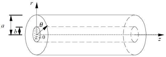
Figure 1.
Infinitely long straight fluid filled pipeline model.
In the following, the displacement scalar potential function is denoted by , the vector potential function by , the longitudinal-wave velocity in the wall by , the shear-wave velocity by , the shear modulus of the pipe wall material by , the wave velocity in the liquid in the pipe by , and the liquid density in the pipe by . Some previous studies have assumed an axisymmetric source in a plate [32] or in a pipe, using a cylindrical coordinate system [33], while some have assumed a point source [34,35]. In the present study, the assumption of axisymmetric excitation is an important one. Under axisymmetric excitation, with , the wave equation in the wall can be represented by the following equations for two scalar potential functions:
where
The radial and axial components of the displacement are
where is the radial components of the displacement in the wall, is the axial components of the displacement in the wall, and the normal and tangential components of the stress are
where is the normal component of the stress in the wall, is the tangential components of the stressin the wall, and are the Lame coefficients.
Under the assumption of a simple harmonic vibration in the direction, the displacement potential function can be expressed as
With the time dependence ignored, by substitution of these expressions into the wave equation, the relationship between the displacement potential function and the displacement and stress in the pipe wall can be obtained.
When , the formal solution for the potential function in the wall is
where A, B, C, and D are constants.
The wave equation satisfied by the water potential function is
The radial and axial components of the displacement in the water are
where is the radial component of the displacement in the water, is the axial component of the displacement in the water.
The normal stress in the water is
where is the normal stress in the water.
Similarly, under the assumption of a simple harmonic vibration in the direction, the displacement potential function can be expressed as
With the time dependence ignored, on substitution of these expressions into the wave equation, the relationship between the displacement potential function and the displacement and stress in the water can be obtained.
When , the formal solution for the potential function in the water is
where E is a constant. The boundary conditions are
Substitution of the formal solutions from Equations (4) and (10) into the expressions for the stress and displacement, and substitution into the boundary conditions (9), then gives the eigenequation
where
2.2. Calculation of the Normal Frequency
For Equation (10) to have a nonzero solution, the determinant of the coefficient matrix must vanish, i.e.,
This equation is the dispersion relation.
If , then , , and , and there is no sound propagation in the axial direction of the pipeline. Then, can be obtained by substituting these values of , , and into Equation (11), and the corresponding frequency is the normal frequency of the corresponding order of vibration of the fluid-filled elastic pipeline.
Table 1 shows an example of the normal frequencies of the first four orders of vibration calculated using Newton’s iterative method with the wall parameters of the experimental liquid-filled PE pipeline (also shown in the table).

Table 1.
Wall material parameters of the experimental polyethylene (PE) pipeline and an example of the numerically calculated normal frequencies.
2.3. Axial and Radial Dependence of the Sound Field
The sound field in the tube can be analyzed in terms of the formal solution in Equation (8) for the displacement potential function in the water. If the radial wavenumber is negligible, then only the axial dependence of the wave needs be considered. When is real, is a periodic function, and the sound wave is able to propagate for long distances along the axial direction. When is imaginary, is an exponential function, and the normal wave is transformed into a nonuniform wave attenuated according to an exponential law along the axial direction, and thus has very little influence on the sound field far from the pipeline axis: The sound wave cannot propagate for long distances in the pipeline.
If the axial wavenumber is negligible, then only the radial dependence of the wave needs be considered. It can be seen that this is given by the zeroth-order Bessel function , and so the sound pressure is greatest close to the axis.
3. Experimental Apparatus and Procedure
To verify the theoretical results, experiments were carried out using the system shown in Figure 2. These experiments focused on the distribution of the sound field and the acoustic propagation behavior in the pipeline for different excitation sources when the liquid in the pipeline was stationary. The experimental conditions are listed in Table 2, and photographs of the experimental conditions and experiment apparatus are shown in Figure 3.
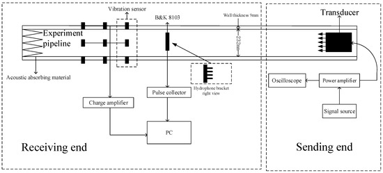
Figure 2.
Experimental system for investigating acoustic propagation characteristics of a fluid-filled PE pipeline.
Table 2.
Experimental conditions.
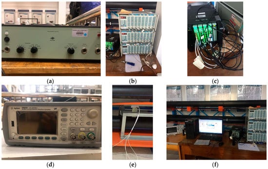
Figure 3.
Experimental apparatus and acquisition system: (a) B&K2713 power amplifier; (b) YE5859 charge amplifier; (c) B&K pulse collector; (d) Agilent 33522A signal source; (e) hydrophone bracket; (f) experimental acquisition system.
Normal waves in the pipeline can be analyzed under white noise conditions. The white noise frequency range was selected as 0–20 kHz according to the sampling frequency of the collector and the theoretically calculated normal frequency. The variation of the sound field along the axial direction in the pipeline can be analyzed under a single-frequency-signal condition. The two frequencies below and above the cutoff frequency were selected in experimental conditions 2 and 3, respectively, to verify the cutoff effect of the sound in the pipeline. Single-frequency mechanical excitation corresponds to the acoustic signal experimental conditions, and the propagation path of the sound was analyzed along the axial direction, and therefore experimental conditions 4 and 5 involved transmission of two single-frequency mechanical force signals of the same frequency as the sound source.
The maximum sampling rate of the B&K pulse collector was 131,072 Hz. The sensors used in this experiment were a B&K8103 hydrophone and B&K4371 vibration sensor. Their specifications are given in Table 3.
Table 3.
Specifications of sensors.
As mentioned in references [10,11,12,13], there have been many experimental investigations of acoustic propagation in fluid-filled elastic pipelines; however, these pipelines were rather short, and there was no special treatment of the end of the pipeline other than, in some cases, the simple addition of a flange, which caused inverse superposition of the sound field in the axial direction. These previous experiments used a single hydrophone, measuring the sound pressure spectrum at a single point only, and therefore it was not possible to obtain the distribution of the sound field along the entire pipeline.
To avoid the above problems, in the present experiment, an 18-m-long PE pipeline with two layers of anechoic tips of different lengths installed at the end was used, which completely eliminated echo and prevented inverse superposition of the sound field in the axial direction. As the source, a piston transducer was mounted on the front of the pipe through a flange, and vibration isolation material was interposed between the flange and the pipeline, thereby preventing direct excitation of the pipe wall. The wall parameters were the same as those used in the theoretical calculations (see Table 1). Five slots, each of length 1 m, in the axial direction were cut in the pipe wall at a distance of 1 m from the transducer, with a 1 m gap between them (see Figure 4).
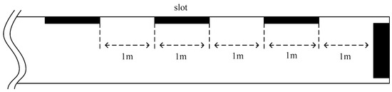
Figure 4.
Slots of the pipeline.
Four 8103 hydrophones were mounted on a bracket, and so the sound pressure at four different radial positions could be measured at the same time, as shown in Figure 2. The hydrophone bracket was made from polyvinyl chloride (PVC), which has characteristic impedance similar to that of water, greatly reducing the scattering of sound waves as they passed through the bracket. Three other hydrophones measured the near-field signal at 0, 0.05, 0.1, and 0.15 m from the axial center of the transducer. After the pipeline was filled with water, it was allowed to stand for more than 30 h to eliminate the effect of bubbles on the experiment.
After the fluid column (water) was excited by the transducer, the hydrophones were moved along the axial slots away from the source, and recordings were taken at 10 cm intervals; thus, each slot had 9 or 10 recording points. The use of the hydrophone bracket ensured that the radial positions of the hydrophones remained unchanged when the axial position was changed. In this way, the sound pressure distributions of the fluid column along both the axial and radial directions were measured.
The analysis bandwidth of the collector was set to 0–25 600 Hz, in accordance with the theoretical normal frequencies, and the corresponding sampling frequency was set to 65,536 Hz by the Nyquist law, with a sampling time of 10 s. The power spectrum of the corresponding working condition was obtained through fast Fourier transform (FFT) processing of the time-domain signal. To determine the propagation path of the sound in the experimental system and compare it with the acoustic signal of the fluid in the pipeline at the same time, the vibration of the wall was also measured in this experiment. There were three rows of vibration sensors encircling the outside of the wall, each with four sensors, with a separation of 0.33 m between each row.
The deployment of the hydrophones and vibration sensors and the corresponding labels are shown in Figure 5.
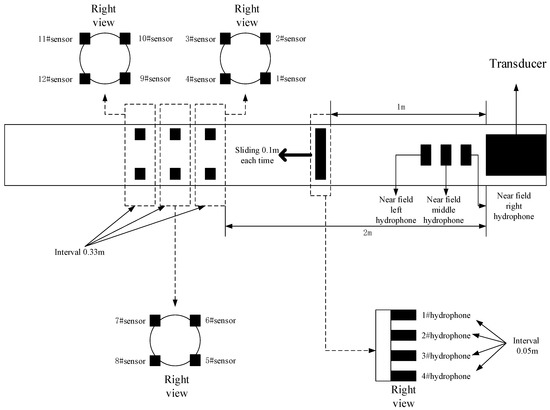
Figure 5.
Deployment and labeling of hydrophones and vibration sensors.
4. Results and Discussion
4.1. Behavior of Normal Waves in the Pipeline
For working condition 1, the transmitting voltage level response of the transducer is shown in Figure 6. The measurement results from the hydrophones at different positions along the axial direction in the pipeline are shown in Figure 7. It can be seen that the acoustic signal in the pipeline exhibits a significant cutoff phenomenon, with a cutoff frequency of 4.7 kHz, which is close to the theoretically determined cutoff frequency of 4.6 kHz.
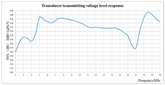
Figure 6.
Transmitting voltage level response of transducer.
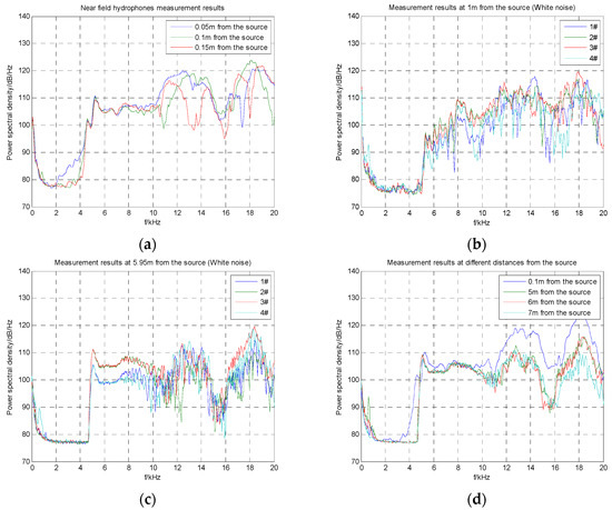
Figure 7.
Measurement results from hydrophones at different positions along the axial direction under white noise excitation: (a) 0.05, 0.1, and 0.15 m from the source; (b) 1.1 m from the source; (c) 5.95 m from the source; (d) 0.1, 5, 6, and 7 m from the source.
The sound energy of the far field can be divided into four intervals from the spectrum: (1) Below 4.7 kHz; (2) 4.7–10.6 kHz; (3) 10.6–16 kHz; (4) 16 kHz and above. The boundary points of these intervals are the frequencies of the normal wave in the pipeline, which are basically consistent with the calculated frequencies of the corresponding orders, as shown in Table 4.
Table 4.
Comparison of calculated and experimental normal frequencies.
As mentioned before, the experimental pipeline is slotted. PE is not a very rigid material and, as a result of the slotting process, the tube is deformed radially. This is the main reason for the error between the actual measured frequency and the theoretically calculated frequency. In addition, the parameters in Table 1 are the material elastic parameters of standard high-density PE, which are not necessarily exactly the same as those of the wall of the experimental pipeline, which also leads to an error between the theoretical and experimental results.
In interval (1), the curve of the power spectrum is very close to the background noise. Close to 4.7 kHz, however, the curve suddenly rises, exhibiting a cutoff phenomenon. Then, in interval (2), the curve changes relatively gently, which is basically consistent with the corresponding frequency band of the transmitting transducer frequency response curve. As the distance between the measurement points and the source becomes greater, it can be seen that the curve decreases monotonically; in interval (3), the curve changes more sharply, and many resonance peaks appear. As the frequency increases, the distance between adjacent peaks also increases, and the appearance of the curve in interval (4) is similar to that in interval (3).
In terms of the behavior of the normal wave, interval (1) is below the cutoff frequency, and the normal wave is attenuated exponentially in the axial direction. The curve of the power spectrum in this frequency band is basically the same as the background, and it can be seen that the power spectrum decays exponentially with frequency in the near field.
Interval (2) lies between the first-order and second-order normal wave frequencies; only the first-order normal wave can propagate, and the curve of the power spectrum hardly changes with frequency. The trend in this section of the curve is related to the transmitting response of the source, with the curve monotonically decreasing along the axial direction as a result of absorption of sound waves by the tube wall.
The first and second orders of the normal wave propagate simultaneously in interval (3), and the first, second, and third orders propagate in interval (4), where there is strong interference leading to large fluctuations in the curve and to the appearance of many resonant peaks.
The results of the vibration signal measurements are shown in Figure 8. The frequency response of the vibration signal is similar to that of the acoustic signal in its overall trend, with a cutoff phenomenon, and the division of the modal frequencies of each order is obvious. The vibration signal in the frequency band above the cutoff frequency is transmitted from the acoustic signal in the water.
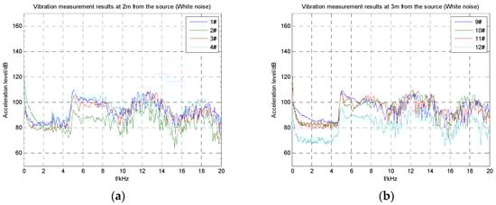
Figure 8.
Measurement results from vibration sensors on the outside of the pipeline wall: (a) 2 m from the source; (b) 3 m from the source.
4.2. Variation of the Sound Field along the Axial Direction
The variation of the sound field along the axial direction can be seen more clearly from analysis of the response to a single-frequency source compared with the response to the white noise in working condition 1. In working conditions 2 and 3, two representative single-frequency signals were used, 4.2 and 5.2 kHz, which are respectively below and above the cutoff frequency. The main frequency power spectrum was obtained as an average of the measurements by the four hydrophones on the bracket, and its variation along the axial distance is shown in Figure 9. It can be seen from Figure 9a that for a source frequency below the cutoff frequency, the power spectrum of the main frequency is attenuated very rapidly, indeed exponentially, as the distance increases. Acoustic signals below the cutoff frequency cannot propagate axially over long distances in the pipeline. For a source frequency above the cutoff frequency, as shown in Figure 9b, the power spectrum of the main frequency hardly changes with distance. There is only 4 dB attenuation from 3 to 10 m, and this attenuation is a result of acoustic absorption by the pipeline wall.
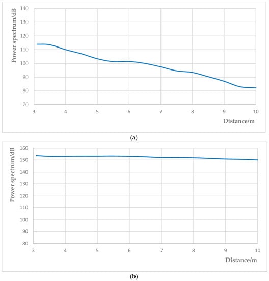
Figure 9.
Variation of the main frequency average power spectrum along the axial direction: (a) 4.2 kHz source; (b) 5.2 kHz source.
4.3. Variation of the Sound Field along the Radial Direction
To explore the variation of the sound field in the radial direction, measurements were performed before and after the hydrophone bracket was raised by 1.5 cm, as shown schematically in Figure 10. The results of these measurements are shown in Figure 11.
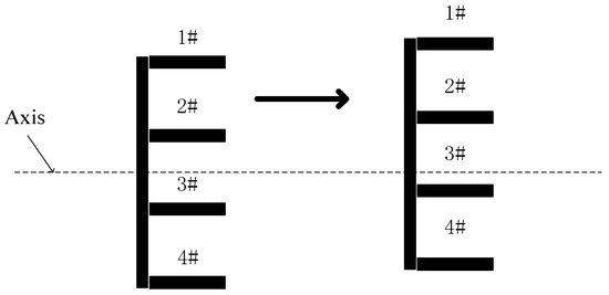
Figure 10.
Raising of hydrophone bracket.
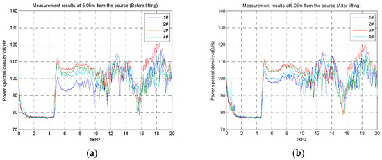
Figure 11.
Results of hydrophone measurements at different depths 5.05 m from the source: (a) Before and (b) after lifting of hydrophone bracket.
The frequency band between the first- and second-order normal frequencies was analyzed. Before lifting, the 2# and 3# hydrophones were at the same distance from the axis, and similarly for the 1# and 4# hydrophones. Therefore, in Figure 11a, the curves of the power spectra from the 2# and 3# hydrophones are the same, as are those from the 1# and 4# hydrophones. After lifting, the 3# hydrophone is nearest to the axis, followed in order by the 2#, 4#, and 1# hydrophones, which is consistent with the increasing strengths of the respective power spectra. This is in accordance with the theoretical radial dependence on the Bessel function in Equation (8).
The following is a quantitative analysis of the radial distribution. The distance between each pair of hydrophones is 50 mm, and the hydrophone bracket is initially at the radial center position. After lifting, the distances of the 3#, 2#, 4#, and 1# hydrophones from the axis are 10, 40, 60, and 90 mm, respectively. At the cutoff frequency, , depending on the distance from the axis, the theoretical differences between the sound pressure self-spectrum measured by the 3# hydrophone and those measured by the other three hydrophones can be calculated, and the results are compared with the experimental measurements in Table 5. For convenience of exposition, the distance between the 3# hydrophone and the axis is set as , and the differences between the sound pressure power spectrum of the 1#, 2#, and 4# hydrophones and the 3# hydrophone as , , and respectively.
Table 5.
Comparison of hydrophone measurements and theoretical values at different radial locations.
There is good agreement between theory and experiment, and the radial distribution of the normal wave in the tube is quantitatively confirmed to follow the Bessel function behavior.
The reasons for the error are as follows. In the experiment, the magnitude of the lifting was controlled manually, and not very accurately, which is the main source of error: If the lifting range were slightly larger, and the 3# and 4# hydrophones closer to the axis, the amplitude would be higher. If the 1# and 2# hydrophones were further away from the axis, the amplitude would be smaller, which would lead to an increase in ; according to the properties of the Bessel function, the closer the value of the function is to the axis, the slower is its rate of change. Therefore, the power spectrum at the 4# hydrophone would increase more if it were lifted, so the value of would be reduced. If the 1# hydrophone were closer to the upper slot and the outside medium were air (which can be regarded as an absolutely soft boundary), the sound would be totally reflected, so the amplitude would become higher, leading to a decrease in . In addition, the radial deformation of the pipeline due to slotting, scattering by the hydrophone bracket, and the fact that the orientation of the hydrophone was not strictly in the axial direction are all possible sources of error.
4.4. Measurements under Mechanical Excitation
Working conditions 4 and 5 use mechanical force excitation from outside the pipeline wall in a position directly under that of the sound source in the previous working conditions, as shown in Figure 12. Corresponding to working conditions 2 and 3, the single frequencies of excitation applied in working conditions 4 and 5 are 4.2 and 5.2 kHz, respectively. The measurement results from the hydrophones and vibration sensors are shown in Figure 13, Figure 14, Figure 15 and Figure 16. In contrast to the response of the acoustic signal, the excitation of the exciter to the pipe wall was a single-point excitation. Therefore, when the sound propagated mainly along the wall, the sound source excitation and the exciter excitation had completely different radial distribution laws. When the sound propagated mainly along the liquid in the tube, both had the same radial distribution. This is an important basis for judging the propagation path of sound in a pipeline.
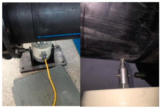
Figure 12.
Exciter and excitation point in working conditions 4 and 5.
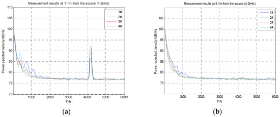
Figure 13.
Mechanical excitation at a single frequency of 4.2 kHz. Measurement results from hydrophones at different distances from the excitation point: (a) 1.1 m; (b) 5.1 m.
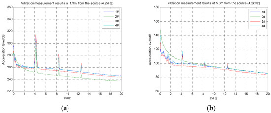
Figure 14.
Mechanical excitation at a single frequency of 4.2 kHz. Measurement results from vibration sensors at different distances from the excitation point: (a) 1.3 m; (b) 5.3 m.
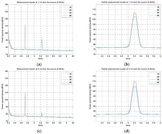
Figure 15.
Mechanical excitation at a single frequency of 5.2 kHz. Measurement results from hydrophones at different distances from the excitation point: (a) 1.1 m; (b) 1.1 m (local); (c) 5.1 m; (d) 5.1 m (local).
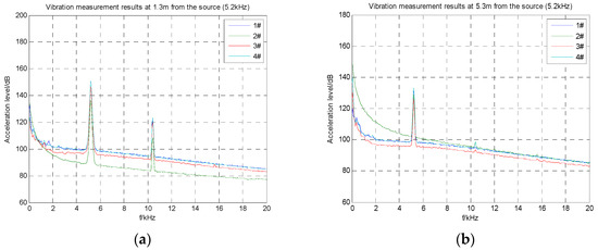
Figure 16.
Mechanical excitation at a single frequency of 5.2 kHz. Measurement results from vibration sensors at different distances from the excitation point: (a) 1.3 m; (b) 5.1 m.
Even if the pipeline wall is excited by a mechanical force, an acoustic signal below the cutoff frequency cannot propagate a long distance in the case of weak excitation. It can be seen from Figure 13b that the hydrophones 5.1 m from the excitation point have difficulty in picking up a signal. In Figure 13a, the acoustic signal at the main frequency exhibits a radial dependence that is different from the Bessel function: The hydrophone near the lower outer wall close to the excitation point receives a stronger signal.
From the vibration measurement results in Figure 14, it can be seen that a vibration signal at the main frequency can still be measured on the wall at 5.3 m, but it is attenuated compared with the measurement from the sensor at 1.3 m, and the hydrophones in the pipeline are unable to detect any signal at 5.3 m. It can be deduced that the signal at 4.2 kHz is propagated mainly through the pipe wall in the form of vibrations. The second and third peaks in Figure 14 result from frequency doubling. The exciter generates frequency doubling when transmitting a single-frequency signal, which is a consequence of its own physical structure and has no effect on the results of this experiment.
For excitation at 5.2 kHz, which is above the cutoff frequency, Figure 15a,b shows the measurement results from hydrophones 1.1 m from the excitation point, and Figure 15c,d those from hydrophones 5.1 m from the excitation point, with Figure 15b,d being partial displays of the frequency band near the main frequency shown in Figure 15a,c, respectively. Figure 16 shows the measurement results from the wall vibration sensors 1.3 and 5.3 m from the excitation point.
The sound power at the main frequency suffers almost no attenuation in the axial direction from 1.1 to 5.1 m, and conforms to the Bessel function dependence in the radial direction. It can be deduced that the signal at 5.2 kHz is propagated mainly in the form of sound through the fluid in the pipeline.
5. Conclusions
The first four orders of normal frequencies in a fluid-filled PE pipeline were calculated, and the distributions of sound in the axial and radial directions were analyzed. The acoustic propagation characteristics of such a pipeline were also studied in an experimental system.
Both the theoretical and experimental investigations have revealed the following:
- Sound in a fluid-filled PE pipeline propagates through the pipeline with the normal frequency at each order.
- Sound above a certain cutoff frequency can propagate in the axial direction of the pipeline for long distances, whereas sound below the cutoff frequency is attenuated exponentially in the axial direction and cannot propagate over long distances.
- In the fluid in the pipeline, the sound power is highest at the axial center and decreases with radial distance from the axial center according to a Bessel function dependence .
- Sound above the cutoff frequency is propagated mainly through the fluid, while sound below the cutoff frequency propagates in the form of vibrations along the pipe wall.
- Controlling and reducing the vibration of the pipe wall is the most effective way to reduce low-frequency noise in a fluid-filled pipeline system.
Author Contributions
Conceptualization, Q.L. and J.S.; methodology, Q.L.; software, J.S.; data validation, J.S.; formal analysis, D.S.; writing—original draft preparation, J.S.; writing—review and editing J.S. and D.S.; supervision and project administration, Q.L.
Funding
This research was funded by Acoustic Science and Technology Laboratory, Harbin Engineering University (SSJSWDZC2018010) and by the National Science Foundation of China (11874131).
Conflicts of Interest
The authors declare no conflict of interest.
References
- Serebrennikov, A.; Serebrennikov, D. Mathematical model of polyethylene pipe bending stress state. Mater. Sci. Eng. 2017, 327, 1–6. [Google Scholar] [CrossRef]
- Gao, Y.; Liu, Y.Y. Theoretical and experimental investigation into structural and fluid motions at low frequencies in water distribution pipes. Mech. Syst. Signal Process. 2017, 90, 126–140. [Google Scholar] [CrossRef]
- Wen, J.H.; Shen, H.J.; Yu, D.L.; Wen, S.X. Theoretical and experimental investigation of flexural wave propagating in a periodic pipe with fluid-filled loading. Chin. Phys. Lett. 2010, 27, 11. [Google Scholar]
- Rayleigh, J.W.S. The Theory of Sound; Dover Publications: New York, NY, USA, 1945. [Google Scholar]
- Scott, J.F.M. The free modes of propagation of an infinite fluid-loaded thin cylindrical shell. J. Sound Vib. 1988, 125, 241–280. [Google Scholar] [CrossRef]
- Sinha, B.K.; Piona, T.J.; Kostek, S. Axisymmetric wave propagation in fluid-loaded cylindrical shells. I. Theory. J. Acoust. Soc. Am. 1992, 92, 1132–1143. [Google Scholar] [CrossRef]
- Sinha, B.K.; Piona, T.J.; Kostek, S. Axisymmetric wave propagation in fluid-loaded cylindrical shells. II. Theory versus experiment. J. Acoust. Soc. Am. 1992, 92, 1144–1155. [Google Scholar] [CrossRef]
- Guo, Y.P. Approximate solutions of the dispersion equation for fluid-loaded cylindrical shells. J. Acoust. Soc. Am. 1994, 95, 1435–1440. [Google Scholar] [CrossRef]
- Xi, Z.C.; Liu, G.R.; Lam, K.Y. Dispersion and characteristic surfaces of waves in laminated composite circular cylindrical shells. J. Acoust. Soc. Am. 2000, 108, 2179–2186. [Google Scholar] [CrossRef]
- Junger, M.C. Radiation loading of cylindrical and spherical surfaces. J. Acoust. Soc. Am. 1952, 24, 288–298. [Google Scholar] [CrossRef]
- Junger, M.C. Vibration of elastic shells in a fluid medium and the associated radiation of sound. J. Appl. Mech. 1952, 19, 439–445. [Google Scholar]
- Junger, M.C. The physical interpretation of the expression for an outgoing wave in cylindrical coordinates. J. Acoust. Soc. Am. 1953, 25, 40–53. [Google Scholar] [CrossRef]
- Muggeridge, D.B.; Buckley, T.J. Flexural vibration of orthotropic cylindrical shells in a fluid medium. AIAA J. 1979, 17, 1019–1022. [Google Scholar] [CrossRef]
- Lamb, H. On the velocity of sound in a tube, as affected by the elasticity of the walls. Manch. Mem. 1898, 42, 1–16. [Google Scholar]
- Lin, T.C.; Morgan, G.W. Wave propagation through fluid contained in a cylindrical elastic shell. J. Acoust. Soc. Am. 1956, 28, 1165–1176. [Google Scholar] [CrossRef]
- Kwun, H.; Bartels, K.A.; Dynes, C. Dispersion of longitudinal waves propagating in liquid-filled cylindrical shells. J. Acoust. Soc. Am. 1999, 105, 2601–2611. [Google Scholar] [CrossRef]
- Horne, M.P.; Hansen, R.J. Sound propagation in a pipe containing a liquid of comparable acoustic impedance. J. Acoust. Soc. Am. 1982, 71, 1400–1405. [Google Scholar] [CrossRef]
- Pan, H.; Koyano, K.; Usui, Y. Experimental and numerical investigations of axisymmetric wave propagation in cylindrical pipe filled with fluid. J. Acoust. Soc. Am. 2003, 113, 3209–3214. [Google Scholar] [CrossRef]
- Lafleur, L.D.; Shields, F.D. Low-frequency propagation modes in a liquid-filled elastic tube waveguide. J. Acoust. Soc. Am. 1994, 97, 1435–1445. [Google Scholar] [CrossRef]
- Aristegui, C.; Lowe, M.J.S.; Cawley, P. Guided waves in fluid-filled pipes surrounded by different fluids. Ultrasonics 2001, 39, 367–375. [Google Scholar] [CrossRef]
- Baik, K.; Jiang, J.; Leighton, T.G. Acoustic attenuation, phase and group velocities in liquid-filled pipes: Theory, experiment, and examples of water and mercury. J. Acoust. Soc. Am. 2010, 128, 2610–2624. [Google Scholar] [CrossRef]
- Liu, B.Y.; Liu, J.C. Suppression of low frequency sound transmission in fluid-filled pipe systems through installation of an anechoic node array. AIP Adv. 2018, 8, 11. [Google Scholar] [CrossRef]
- Wang, M.; Qiao, G.; He, Y.A. Noise control of fluid-filled pipes. Appl. Acoust. 2003, 22, 35–38. [Google Scholar]
- Zhu, Z.X.; Lee, P.C.; Wang, Z.G. Numerical solution compared with experimental result for sound propagation in ducts. Acta Acust. 1988, 13, 1–8. (In Chinese) [Google Scholar]
- Zhu, Z.X.; Guo, R. A study of noise reduction by anti-sound using bypass in ducts with flow. Acta Acust. 1997, 22, 1–10. (In Chinese) [Google Scholar]
- Zhang, Y.M.; Tang, R.; Li, Q.; Shang, D.J. The low-frequency sound power measuring technique for an underwater source in a non-anechoic tank. Meas. Sci. Technol. 2018, 29, 035101. [Google Scholar] [CrossRef]
- Shang, D.J.; Shang, Q.L.D.J.; Lin, H. Experimental investigation on flow-induced noise of the underwater hydrofoil structure. Acta Acust. 2012, 37, 416–423. (In Chinese) [Google Scholar]
- Lan, K.; He, X.T.; Lai, D.X.; Li, S.G. Radiative energy flux of diffusive supersonic wave in a cylinder. Acta Phys. Sin. 2016, 55, 3789–3795. (In Chinese) [Google Scholar]
- Gao, G.J.; Deng, M.X.; Li, M.L. Modal expansion analysis of nonlinear circumferential guided wave propagation in a circular tube. Acta Phys. Sin. 2015, 64, 184303. (In Chinese) [Google Scholar]
- Wang, C.H.; Cheng, J.C. Nonlinear forced oscillations of gaseous bubbles in elastic microtubules. Acta Phys. Sin. 2013, 62, 114301. (In Chinese) [Google Scholar]
- Tang, W.L.; Wu, Y. Interior noise field of a viscoelastic cylindrical shell excited by the TBL pressure fluctuations: I. Production mechanism of the noise. Acta Acust. 1997, 22, 60–69. (In Chinese) [Google Scholar]
- Haider, M.F.; Giurgiutiu, V. Analysis of axis symmetric circular crested elastic wave generated during crack propagation in a plate: A Helmholtz potential technique. Int. J. Solids Struct. 2018, 134, 130–150. [Google Scholar] [CrossRef]
- Rose, J.L. Ultrasonic Guided Waves in Solid Media; Cambridge University Press: Cambridge, UK, 2014. [Google Scholar]
- Mostafapour, A.; Davoodi, S. A theoretical and experimental study on acoustic signals caused by leakage in buried gas-filled pipe. Appl. Acoust. 2015, 87, 1–8. [Google Scholar] [CrossRef]
- Achenbach, J.A.; Achenbach, J.D. Reciprocity in Elastodynamics; Cambridge University Press: Cambridge, UK, 2003. [Google Scholar]
© 2019 by the authors. Licensee MDPI, Basel, Switzerland. This article is an open access article distributed under the terms and conditions of the Creative Commons Attribution (CC BY) license (http://creativecommons.org/licenses/by/4.0/).