Regularization Factor Selection Method for l1-Regularized RLS and Its Modification against Uncertainty in the Regularization Factor

Abstract
Featured Application
Abstract
1. Introduction
2. Summarize l1-RLS
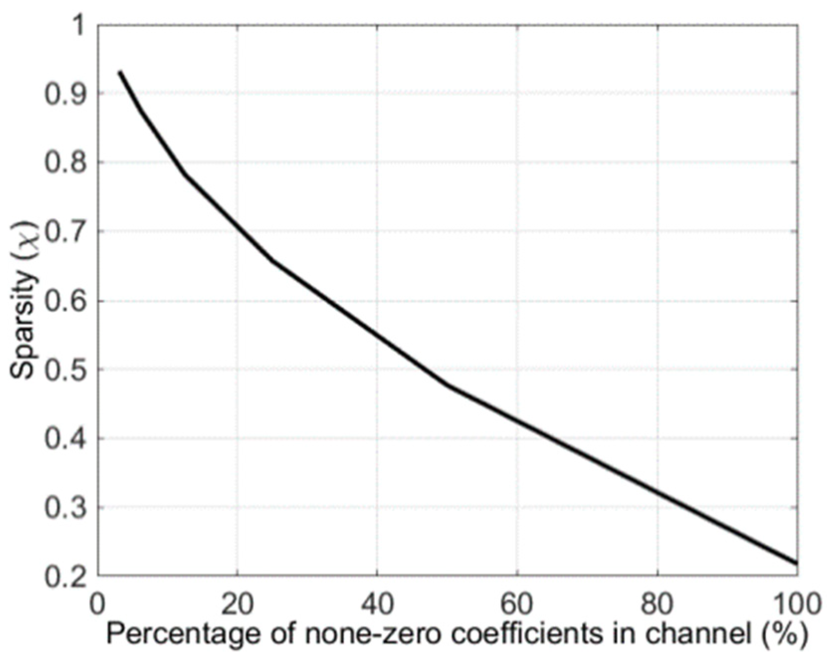
3. Measure of Sparseness
4. New Selection Method in the Sparsity Regularization Constant
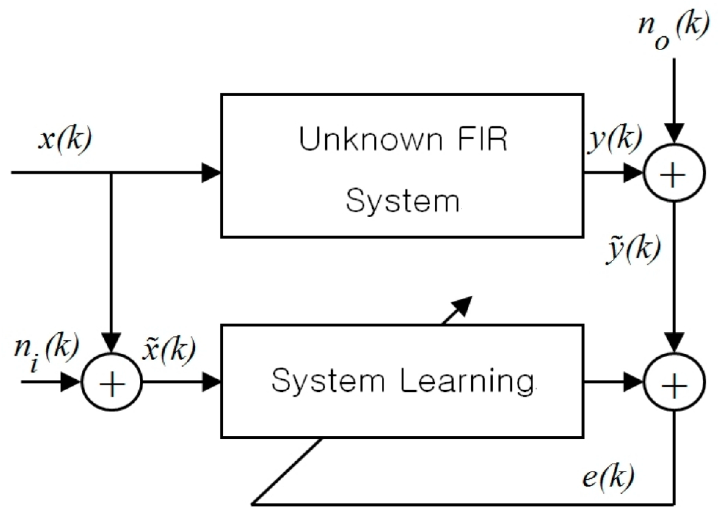
5. New Modeling for l1-RLS with Uncertainty in the Regularization Factor
6. Summarize l1-RTLS for the Solution of l1-RLS with Uncertainty in the Regularization Factor
7. Simulation Results
8. Conclusions
Author Contributions
Funding
Acknowledgments
Conflicts of Interest
References
- Benichoux, A.; Simon, L.; Vincent, E.; Gribonval, R. Convex regularizations for the simultaneous recording of room impulse responses. IEEE Trans. Signal Process. 2014, 62, 1976–1986. [Google Scholar] [CrossRef]
- Merimaa, J.; Pulkki, V. Spatial impulse response I: Analysis and synthesis. J. Audio Eng. Soc. 2005, 53, 1115–1127. [Google Scholar]
- Dokmanic, I.; Parhizkar, R.; Walther, A.; Lu, Y.M.; Vetterli, M. Acoustic echoes reveal room shape. Proc. Natl. Acad. Sci. USA 2013, 110, 12186–12191. [Google Scholar] [CrossRef] [PubMed]
- Remaggi, L.; Jackson, P.; Coleman, P.; Wang, W. Acoustic reflector localization: Novel image source reversion and direct localization methods. IEEE Trans. Audio Speech Lang. Process. 2017, 25, 296–309. [Google Scholar] [CrossRef]
- Baba, Y.; Walther, A.; Habets, E. 3D room geometry interference based on room impulse response stacks. IEEE Trans. Audio, Speech Lang. Process. 2018, 26, 857–872. [Google Scholar] [CrossRef]
- Goetze, S.; Xiong, F.; Jungmann, J.O.; Kallinger, M.; Kammeyer, K.; Mertins, A. System Identification of Equalized Room Impulse Responses by an Acoustic Echo Canceller using Proportionate LMS Algorithms. In Proceedings of the 130th AES Convention, London, UK, 13 May 2011; pp. 1–13. [Google Scholar]
- Yu, M.; Ma, W.; Xin, J.; Osher, S. Multi-channel l1 regularized convex speech enhancement model and fast computation by the split Bregman method. IEEE Trans. Audio Speech Lang. Process. 2012, 20, 661–675. [Google Scholar] [CrossRef]
- Lin, Y.; Chen, J.; Kim, Y.; Lee, D.D. Blind channel identification for speech dereverberation using l1-norm sparse learning. In Proceedings of the Twenty-First Annual Conference on Neural Information Processing Systems, Vancouver, BC, Canada, 3–6 December 2007; pp. 921–928. [Google Scholar]
- Naylor, P.A.; Gaubitch, N.D. Speech Dereverberation; Springer: London, UK, 2010; pp. 219–270. [Google Scholar]
- Duttweiler, D.L. Proportionate normalized least-mean-squares adaptation in echo cancelers. IEEE Trans. Speech Audio Process. 2000, 8, 508–518. [Google Scholar] [CrossRef]
- Gu, Y.; Jin, J.; Mei, S. Norm Constraint LMS Algorithm for Sparse System Identification. IEEE Signal Process. Lett. 2009, 16, 774–777. [Google Scholar]
- Chen, Y.; Gu, Y.; Hero, A.O. Sparse LMS for system identification. In Proceedings of the IEEE International Conference on Acoustics, Speech and Signal Processing, Taipei, Taiwan, 19–24 April 2009; pp. 3125–3128. [Google Scholar]
- He, X.; Song, R.; Zhu, W.P. Optimal pilot pattern design for compressed sensing-based sparse channel estimation in OFDM systems. Circuits Syst. Signal Process. 2012, 31, 1379–1395. [Google Scholar] [CrossRef]
- Babadi, B.; Kalouptsidis, N.; Tarokh, V. SPARLS: The sparse RLS algorithm. IEEE Trans. Signal Process. 2010, 58, 4013–4025. [Google Scholar] [CrossRef]
- Angelosante, D.; Bazerque, J.A.; Giannakis, G.B. Online adaptive estimation of sparse signals: Where RLS meets the l1-norm. IEEE Trans. Signal Process. 2010, 58, 3436–3447. [Google Scholar] [CrossRef]
- Eksioglu, E.M. Sparsity regularised recursive least squares adaptive filtering. IET Signal Process. 2011, 5, 480–487. [Google Scholar] [CrossRef]
- Eksioglu, E.M.; Tanc, A.L. RLS algorithm with convex regularization. IEEE Signal Process. Lett. 2011, 18, 470–473. [Google Scholar] [CrossRef]
- Sun, D.; Liu, L.; Zhang, Y. Recursive regularisation parameter selection for sparse RLS algorithm. Electron. Lett. 2018, 54, 286–287. [Google Scholar] [CrossRef]
- Chen, Y.; Gui, G. Recursive least square-based fast sparse multipath channel estimation. Int. J. Commun. Syst. 2017, 30, e3278. [Google Scholar] [CrossRef]
- Kalouptsidis, N.; Mileounis, G.; Babadi, B.; Tarokh, V. Adaptive algorithms for sparse system identification. Signal Process. 2011, 91, 1910–1919. [Google Scholar] [CrossRef]
- Candes, E.J.; Wakin, M.; Boyd, S. Enhancing sparsity by reweighted minimization. J. Fourier Anal. Appl. 2008, 14, 877–905. [Google Scholar] [CrossRef]
- Lamare, R.C.; Sampaio-Neto, R. Adaptive reduced-rank processing based on joint and iterative interpolation, decimation, and filtering. IEEE Trans. Signal Process. 2009, 57, 2503–2514. [Google Scholar] [CrossRef]
- Petraglia, M.R.; Haddad, D.B. New adaptive algorithms for identification of sparse impulse responses—Analysis and comparisons. In Proceedings of the Wireless Communication Systems, York, UK, 19–22 September 2010; pp. 384–388. [Google Scholar]
- Golub, G.H.; Van Loan, C.F. An analysis of the total least squares problem. SIAM J. Numer. Anal. 1980, 17, 883–893. [Google Scholar] [CrossRef]
- Dunne, B.E.; Williamson, G.A. Stable simplified gradient algorithms for total least squares filtering. In Proceedings of the 34th Annual Asilomar Conference on Signals, Systems, and Computers, Pacific Grove, CA, USA, 29 October–1 November 2000; pp. 1762–1766. [Google Scholar]
- Feng, D.Z.; Bao, Z.; Jiao, L.C. Total least mean squares algorithm. IEEE Trans. Signal Process. 1998, 46, 2122–2130. [Google Scholar] [CrossRef]
- Davila, C.E. An efficient recursive total least squares algorithm for FIR adaptive filtering. IEEE Trans. Signal Process. 1994, 42, 268–280. [Google Scholar] [CrossRef]
- Soijer, M.W. Sequential computation of total least-squares parameter estimates. J. Guid. Control Dyn. 2004, 27, 501–503. [Google Scholar] [CrossRef]
- Choi, N.; Lim, J.S.; Sung, K.M. An efficient recursive total least squares algorithm for raining multilayer feedforward neural networks. Lect. Notes Comput. Sci. 2005, 3496, 558–565. [Google Scholar]
- Lim, J.S.; Pang, H.S. l1-regularized recursive total least squares based sparse system identification for the error-in-variables. SpringerPlus 2016, 5, 1460–1469. [Google Scholar] [CrossRef] [PubMed]
- Lehmann, E. Image-Source Method: MATLAB Code Implementation. Available online: http://www.eric-lehmann.com/ (accessed on 17 December 2018).
- Gay, S.L.; Benesty, J. Acoustic Signal Processing for Telecommunication; Kluwer Academic Publisher: Norwell, MA, USA, 2000; pp. 6–7. [Google Scholar]
- Swanson, D.C. Signal Processing for Intelligent Sensor Systems with MATLAB, 2nd ed.; CRC Press: Boca Raton, FL, USA, 2012; p. 70. [Google Scholar]
- Kuttruff, H. Room Acoustics, 6th ed.; CRC Press: Boca Raton, FL, USA, 2017; p. 168. [Google Scholar]
- Bai, H.; Richard, G.; Daudet, L. Modeling early reflections of room impulse responses using a radiance transfer method. In Proceedings of the IEEE Workshop on Applications of Signal Processing to Audio and Acoustics, New Paltz, NY, USA, 20–23 October 2013; pp. 1–4. [Google Scholar]


| Step 1 | Sparsity: [20] where is the length of the impulse response. |
| Step 2 | |
| Step 3 |
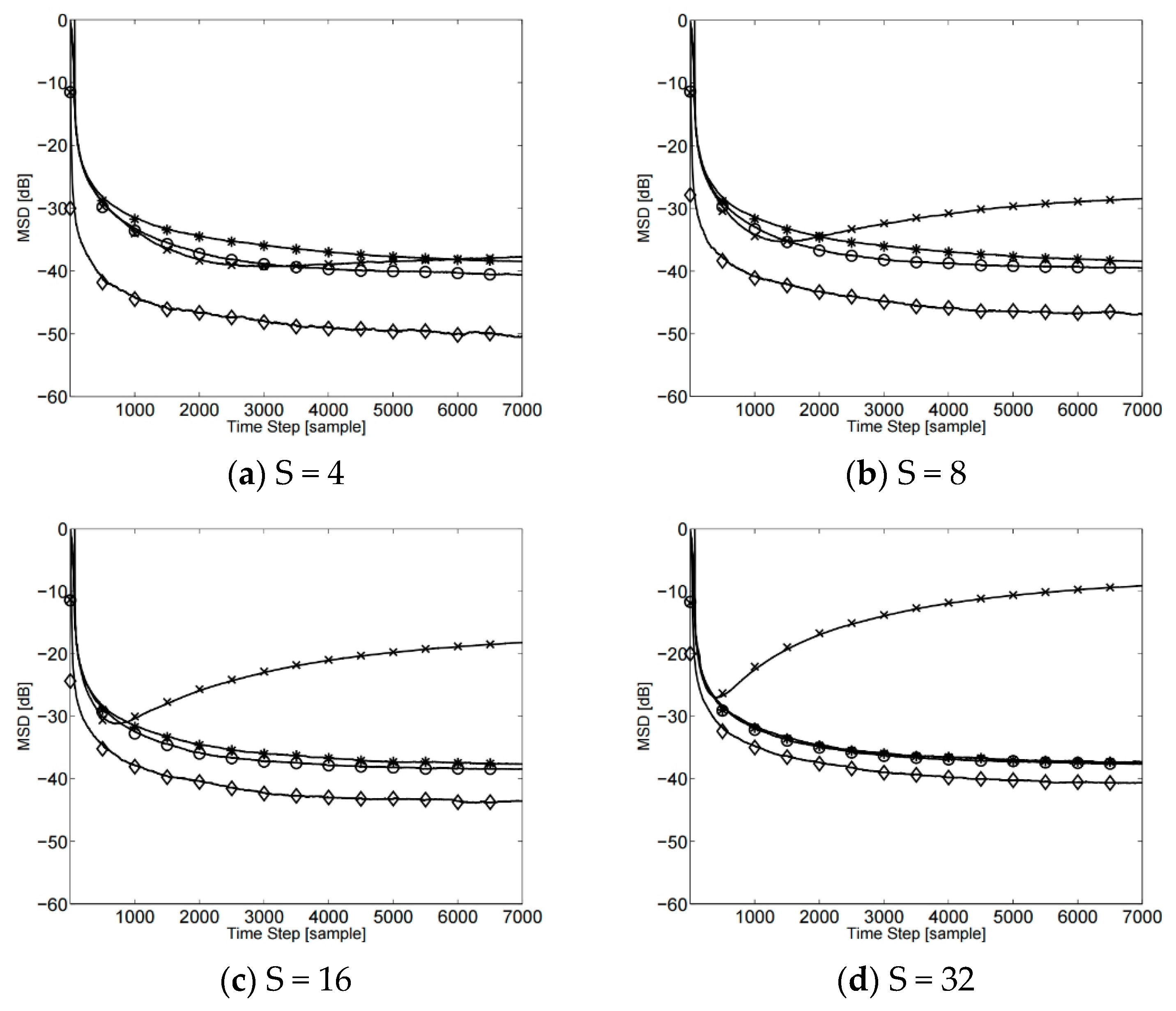
| Sparsity (S) | Algorithm | MSD |
|---|---|---|
| 4 | l1-RLS with the true channel | −40.6 dB |
| l1-RLS with the new method | −37.8 dB | |
| proposed l1-RTLS with the new method | −38.5 dB | |
| Oracle-RLS | −50.4 dB | |
| 8 | l1-RLS with the true channel | −39.5 dB |
| l1-RLS with the new method | −28.4 dB | |
| proposed l1-RTLS with the new method | −38.5 dB | |
| Oracle-RLS | −46.9 dB | |
| 16 | l1-RLS with the true channel | −38.4 dB |
| l1-RLS with the new method | −18.2 dB | |
| proposed l1-RTLS with the new method | −37.6 dB | |
| Oracle-RLS | −43.6 dB | |
| 32 | l1-RLS with the true channel | −37.6 dB |
| l1-RLS with the new method | −9.1 dB | |
| proposed l1-RTLS with the new method | −37.3 dB | |
| Oracle-RLS | −40.6 dB |
| Reverberation Time (T60) | Algorithm | MSD |
|---|---|---|
| 100 ms | l1-RLS with the true channel | −38.5 dB |
| l1-RLS with the new method | −34.7 dB | |
| proposed l1-RTLS with the new method | −35.4 dB | |
| Oracle-RLS | −45.3 dB | |
| 400 ms | l1-RLS with the true channel | −32.1 dB |
| l1-RLS with the new method | −20.9 dB | |
| proposed l1-RTLS with the new method | −30.1 dB | |
| Oracle-RLS | −36.0 dB |
© 2019 by the authors. Licensee MDPI, Basel, Switzerland. This article is an open access article distributed under the terms and conditions of the Creative Commons Attribution (CC BY) license (http://creativecommons.org/licenses/by/4.0/).
Share and Cite
Lim, J.; Lee, S. Regularization Factor Selection Method for l1-Regularized RLS and Its Modification against Uncertainty in the Regularization Factor. Appl. Sci. 2019, 9, 202. https://doi.org/10.3390/app9010202
Lim J, Lee S. Regularization Factor Selection Method for l1-Regularized RLS and Its Modification against Uncertainty in the Regularization Factor. Applied Sciences. 2019; 9(1):202. https://doi.org/10.3390/app9010202
Chicago/Turabian StyleLim, Junseok, and Seokjin Lee. 2019. "Regularization Factor Selection Method for l1-Regularized RLS and Its Modification against Uncertainty in the Regularization Factor" Applied Sciences 9, no. 1: 202. https://doi.org/10.3390/app9010202
APA StyleLim, J., & Lee, S. (2019). Regularization Factor Selection Method for l1-Regularized RLS and Its Modification against Uncertainty in the Regularization Factor. Applied Sciences, 9(1), 202. https://doi.org/10.3390/app9010202