Adaptive Fuzzy Backstepping Sliding Mode Control for a 3-DOF Hydraulic Manipulator with Nonlinear Disturbance Observer for Large Payload Variation

Featured Application

This article belongs to the Section Mechanical Engineering.

Abstract

The paper proposes an adaptive fuzzy position control for a 3-DOF hydraulic manipulator with large payload variation. The hydraulic manipulator uses electrohydraulic actuators as primary torque generators to enhance carrying payload of the manipulator. The proposed control combines backstepping sliding mode control, fuzzy logic system (FLS), and a nonlinear disturbance observer. The backstepping sliding mode control includes a sliding mode control for manipulator dynamics and a PI control for actuator dynamics. The fuzzy logic system is utilized to adjust the control gain and robust gain of the sliding mode control (SMC) based on the output of the nonlinear disturbance observer to compensate the payload. The Lyapunov approach and backstepping technique are used to prove the stability and robustness of the whole system. Some simulations are implemented, and the results are compared to other controllers to exhibit the effectiveness of the proposed control.

1. Introduction

Nowadays, manipulators are used to assist humans and work in some specific fields such as assembling, industrial application, medical field, exploration, etc. Its high nonlinearity, coupling dynamic reaction, and uncertainties [1] are challenges for control strategy. In order to deal with these problems, some approaches, such as proportional integral derivative (PID) [2,3], backstepping control [4,5], sliding mode control (SMC) [6,7], adaptive control [8,9,10,11], and intelligent control techniques [12,13,14] have been investigated. In these methods, the actuator dynamics are usually excluded to simplify the control design. However, according to [15], they can affect the dynamic characteristic and stability [15,16], as well as dominate the robot dynamics [17]. So, actuator dynamics should be included in control design [16,17,18,19].

Conventionally, electric actuators (EAs) are utilized as primary torque generators in each joint of the manipulator because of owning properties such as excellent accuracy and controllability but suffer from the possibility of sparking [19]. Besides, this approach is not effective when the manipulator operates in wide force/torque range. Pneumatic actuators (PAs) are another potential candidate to replace the electric actuators because of its characteristics [20]. The main advantages of the PAs can be revealed as quick response, high power-to-weight, and power-to-volume ratios [21]. However, according to Tu et al. air compressibility and the elasticity depending on material structure over the time are the main drawbacks to be considered. In addition, the high nonlinearities in the PAs is because its frame degrades the performance of the system [22]. Electro-hydraulic actuators (EHAs) are considered as a good choice to replace the EAs and PAs and are increasingly used in industries because of their high power to weight ratio and high stiffness [23,24]. Nevertheless, the EHAs are complicated and still a big challenge because of their characteristics such as nonlinear and uncertainty parameters. To deal with the uncertainties which exist in the actuator dynamic and guarantee the stability of the system, the backstepping sliding mode control which takes advantage of the sliding surface in strong robustness against perturbation [25,26,27] and backstepping technique in solving both the problem of stabilization and tracking trajectory of nonlinear systems [4,5] and [28,29,30] is exploited.

In practice, the manipulator often works under variant uncertainties or external payload variation, for instance, thus degrading the performance of the robot. To cope with these issues, some techniques have been proposed to improve tracking performance. R. Sharma et al. came up with two-layer fraction order fuzzy logic controller [31,32,33] and mixed locally recurrent neural network [33] with the Cuckoo search algorithm (CSA). By combining with optimization technique to determine the optimal control parameters with the payload, the results indicated that the tracking performance is improved under the presence of the payload. Although the controller parameters are optimized, the experiments must be implemented in several conditions to get enough characteristic data for the optimal algorithm. Several experiments with the change of the system parameters and working conditions must be carried out. Once the experimental conditions are changed or different from characteristic data, the stability of the system cannot be guaranteed. Nho et al. [34] applied fuzzy neural technique to estimate the payload for compensation. The idea is based on the change in acceleration error due to its change in inertia, thus designing a detect algorithm. However, according to the author, the network was trained off-line. This implies that the experimental data must be sufficient to characterize the system. Fuzzy logic system (FLS) has shown a great performance and considered as a powerful tool to be back up in various system applications [35,36]. FLS, its laws are designed based on some knowledge about the control system, with adaptive laws can overcome the system parameters variation, as well as adjust the controller gains. Some studies such as Sharkawy et al. in [37], Amer et al. in [38], He et al. in [39], and Guo et al. in [40] employed FLS with online-tuning for adjusting the controller gains to adopt with the manipulator behavior. Their results have shown an improvement in performance when applying adaptive laws. However, in those reports, the payload is supposed to be well-known or the uncertainties are supposed to be bound. Unfortunately, in practice, these uncertainties/payloads maybe randomly changed and cannot be exactly measured.

According to the above reports, this paper employed the FLS for adjusting the control feedback gains to improve the manipulator performance with the unknown variant payload. To overcome this issue and achieve higher performance, we suggest using disturbance observer (DO) [41,42,43] to detect the change of the external payload mass.

Based on the above reasons, we consider a 3-DOF hydraulic manipulator with unknown payload to verify the proposed algorithm. Compared with the existing work, the main contributions of this study are highlighted as follows:

-

First, the dynamics of the 3-DOF hydraulic manipulator including actuator is derived.

-

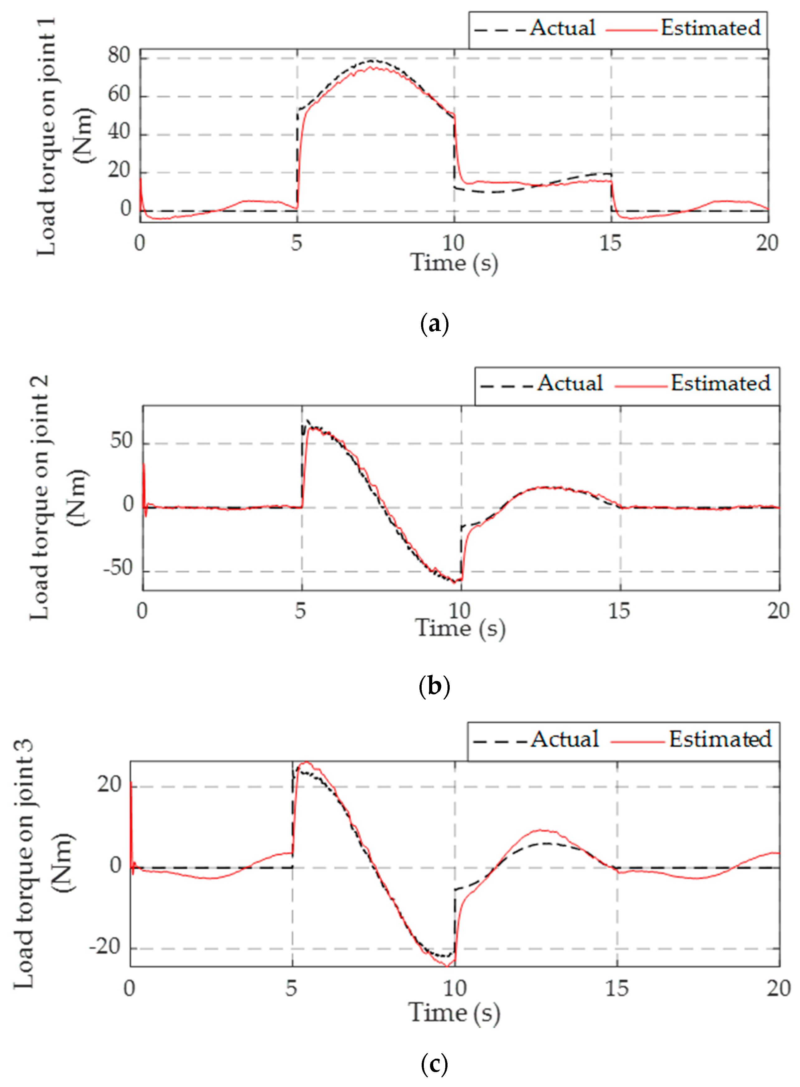
Second, the backstepping sliding mode control is proposed for the tracking performance and the disturbance observer (DO) is utilized to observe the variation of the external payload torque.

-

Third, the two FLS is used to adopt the system performance. The first FLS is applied for tuning switching gain based on its tracking error and error changing rate. The other FLS is used to boost the controller gains with the input is the estimated load torque.

-

Finally, some simulated comparisons are given between the proposed controller scheme and the conventional controller to demonstrate the effectiveness of the proposed algorithm.

This paper is organized as follows: Section 2 presents the manipulator dynamics including EHAs. The motion of the manipulator in Cartesian space, as well as joint space and actuator-space, is discussed in this section. The proposed algorithm for the system is designed with the proof of the stability and robustness by using Lyapunov theory depicted in Section 3. Section 4 provides some simulation results and experimental results are discussed in Section 5. Conclusion and future work are presented in Section 6.

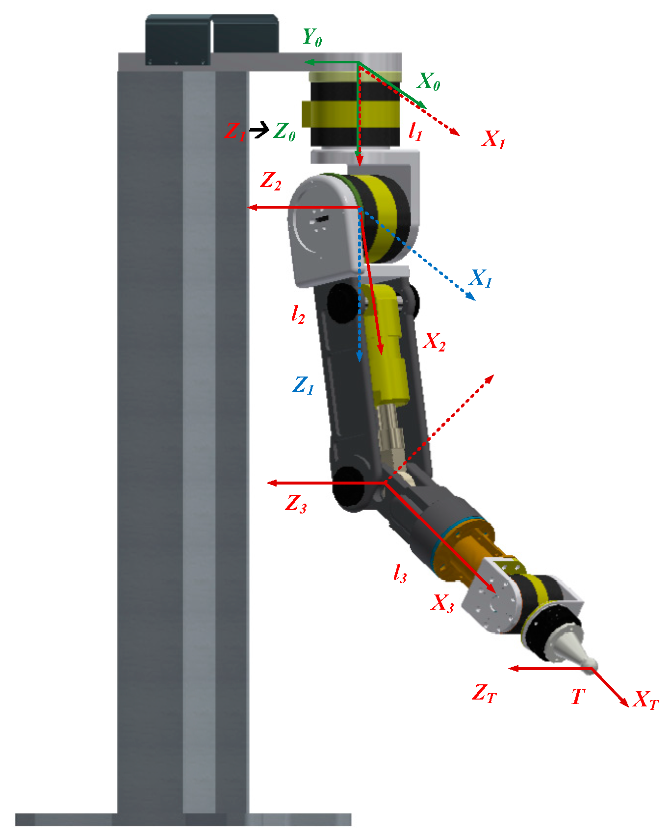
2. Manipulator Analysis

The hydraulic robot is illustrated in Figure 1. Each part of this manipulator is driven by a hydraulic rotary actuator (HRA) controlled by using servo valve. The behavior of the manipulator via actuator dynamic is analyzed elaborately.

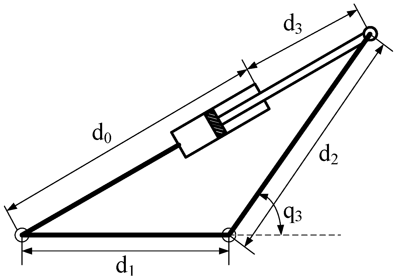
2.1. Dynamics Manipulator

The dynamics of the robot with a degree of freedom can be expressed as:

$$M(q)\ddot{q}+C(q,\dot{q})\dot{q}+G(q)+F_d\dot{q}+F_s\left(\dot{q}\right)=\tau +{\tau }_{load}$$

(1)

where $q,\dot{q},\ddot{q}\in R^3$ are position, angular velocity, and angular acceleration vectors of each joint, respectively, $M(q)\in R^{3\times 3}$ is the symmetric and positive definite matrix of inertia, $C(q,\dot{q})\in R^{3\times 3}$ denotes the Coriolis and Centrifugal term matrix, $G(q)\in R^3$ is the gravity term, τ is torque acting on joints, $F_d\in R^{3\times 3}$ is a diagonal matrix of viscous and dynamic friction coefficients, $F_s\left(\dot{q}\right)\in R^n$ is the vector of unstructured friction effects such as static friction terms, ${\tau }_{load}$ denotes the torque load induced by an external payload. However, the dynamics of the manipulator is difficult to determine clearly because of the mass distribution, and oscillation in the process of operation. Then the Equation (1) is re-written as:

$$\widehat{M}(q)\ddot{q}+\widehat{C}(q,\dot{q})\dot{q}+\widehat{G}(q)+d=\tau +{\tau }_{load}$$

(2)

where $\widehat{M}(q)\ddot{q}+\widehat{C}(q,\dot{q})\dot{q}+\widehat{G}(q)$ represent the estimated terms and can be assumed to be known (Appendix A), $d=\Delta M(q)\ddot{q}+\Delta C(q,\dot{q})\dot{q}+\Delta G(q)+F_s\left(\dot{q}\right)+\Delta F_d\dot{q}\in R^3$ is the vector of any generalized input because of uncertainties, disturbances, or un-modeled dynamic. The detailed structure of the $\widehat{M}(q),\widehat{C}(q,\dot{q}),\widehat{G}(q)$ is discussed in Appendix A.

Assumption 1.

All$\Delta (.)$are bounded, i.e.,${\Vert \Delta (.)\Vert }_{\infty }\le \xi (.)$.

Unlike conventional manipulator, the last link of our proposed hydraulic manipulator employs cylinder to load heavier object. The torque acting on the joint is essentially induced by the force generated by the cylinder then the relationship between the rotational motion of the joint and the translational motion of the actuator is investigated. The architecture of the last link is illustrated in Figure 2.

The correlation between the motion of the actuator in the actuator space and the motion in joint space can be derived by:

$$d_3+d_0=\sqrt{d_1{}^2+d_2{}^2-2d_1{d}_2\cos \left(\pi -q_3\right)}$$

(3)

where d₀ is the initial length in case of maximum retracting; the positive direction in the actuator space is chosen for extracting the piston. d₃ denotes the position of the end-effector under the motion of the cylinder, d₁ and d₂ are fixed length of the hinge joints.

To obtain the correlational velocity between the actuator and the joint motion, taking the derivation respect to time, the Equation (3) results into:

$${\dot{d}}_3=\frac{\partial d_3}{\partial q_3}{\dot{q}}_3=\frac{d_1{d}_2\sin \left(\pi -q_3\right)}{\sqrt{d_1{}^2+d_2{}^2-2d_1{d}_2\cos \left(\pi -q_3\right)}}{\dot{q}}_3=J_{a3}\left(q_3\right){\dot{q}}_3$$

(4)

where J_a3 (q₃) is a Jacobian matrix of the 3rd joint.

Thus, a torque acting on this joint can be derived as:

$${\tau }_3=J_{a3}^T\left(q_3\right)F_3$$

(5)

The completely correlational motion between the actuator and the joint motion is described by:

$$\left(\begin{array}{c}{\dot{q}}_{1a}\\ {\dot{q}}_{2a}\\ {\dot{d}}_3\end{array}\right)=\left(\begin{array}{ccc}1& 0& 0\\ 0& 1& 0\\ 0& 0& J_{a3}\left(q_3\right)\end{array}\right)\left(\begin{array}{c}{\dot{q}}_1\\ {\dot{q}}_2\\ {\dot{q}}_3\end{array}\right)$$

(6)

where ${\left(\begin{array}{ccc}{q}_{1a}& q_{2a}& d_3\end{array}\right)}^T\in R^3$ denotes position vector of the actuator in actuator space.

2.2. The Dynamic of the Electro-Hydraulic Actuator

The schematic of the EHA is described in Figure 3. The dynamic is presented by the following equation:

$$J_i{\ddot{q}}_{ia}={\tau }_{hydraulic\_i}-b_{act\_i}{\dot{q}}_{ia}-d_{act\_i}(q_{ia},{\dot{q}}_{ia},t)-{\tau }_{load\_i},(i=1,2,3)$$

(7)

where $J_i$ is an inertia mass of the link ith, $q_{ia},{\dot{q}}_{ia},{\ddot{q}}_{ia}$ are the angular position, velocity, and acceleration of the actuator which have a same movement as each link of the manipulator, $b_{act\_i}$ is a coefficient of the viscosity friction, $d_{act\_i}(q_{ia},{\dot{q}}_{ia},t)$ represents uncertainty parameters such as friction or disturbance, ${\tau }_{load\_i}$ is an arbitrary load torque on the actuator ith, and ${\tau }_{hydraulic\_i}$ is torque applied on the link ith of the manipulator, same as Equation (2).

${\tau }_{hydraulic\_i}$ is produced by:

$${\tau }_{hydraulic\_i}=\{\begin{array}{ll}{A}_{q_{ia}}(P_{i1}-P_{i2})=A_{q_{ia}}{P}_{iL}& \left(\mathrm{for}\hspace{0.17em}\mathrm{rotary}\hspace{0.17em}\mathrm{actuator}\right)\\ J_{a3}^T\left(q\right)F_a=J\left(q\right)\left(A_1{P}_1-A_2{P}_2\right)& \left(\mathrm{for}\hspace{0.17em}\mathrm{cylinder}\right)\end{array}$$

(8)

where $A_{q_{ia}}$ is the radian displacement of the rotary actuator, $A_i{}_{\left(i=1,2\right)}$ are an area of the bore side and rod side of the cylinder, respectively. $P_i{}_{\left(i=1,2\right)}={\left[\begin{array}{ccc}{P}_{i1}& \cdots & P_{i3}\end{array}\right]}^T$ are pressure in chamber 1 and chamber 2 of each actuator, respectively.

The pressure in each chamber can be computed by [44]:

$$\frac{d{P}_{i1}}{dt}=\frac{\beta }{V_{i1}}\left(Q_{i1}-A\frac{\partial q_a}{\partial q}\dot{q}\right)-{\zeta }_{i1}\left(t\right)$$

(9)

$$\frac{d{P}_{i2}}{dt}=\frac{\beta }{V_{i2}}\left(-Q_{i2}+A\frac{\partial q_a}{\partial q}\dot{q}\right)+{\zeta }_{i2}\left(t\right)$$

(10)

where $V_{i1}=V_{i01}+A_{i}q$ is the volume of chamber 1, $V_{i2}=V_{i02}-A_{i}q$ is volume of chamber 2, $V_{i01}$ and $V_{i02}$ are the initial volumes of the two chambers, β is the Bulk modulus, $q_{leak}$ is the leakage volume between the two chambers, $Q_{i1}$ is the flow rate supplied by the hydraulic source to the forward chamber, and $Q_{i2}$ is the returned flow rate from the backward chamber. Both $Q_{i1}$ and $Q_{i2}$ are driven by position of the spool inside the servo valve.

The equation expressed in relation between $Q_{i1}$ and $Q_{i2}$ and displacement of the spool are presented in [45,46,47]:

$$Q_{i1}=k_q\sqrt{\frac{2}{\rho }}[sign(x_v)\sqrt{P_S-P_{i1}}+sign(-x_v)\sqrt{P_1-P_{ir}}]$$

(11)

$$Q_{i2}=k_q\sqrt{\frac{2}{\rho }}[sign(x_v)\sqrt{P_{i2}-P_r}+sign(-x_v)\sqrt{P_S-P_{i2}}]$$

(12)

where x_v is the valve displacement, ω is the spool valve area gradient, ρ is the density of the fluid, C_d is the discharge coefficient, P_s and P_r are the supply and return pressure, respectively.

The dynamic of the valve was presented in [48,49]:

$$m_v{\ddot{x}}_v+b_v{\dot{x}}_v+k_v{x}_v=F_{flow}+f(u)$$

(13)

Since $x_v$ relates to the input voltage, and if neglecting servo-valve dynamics [50], we can assume approximately that an input signal u is a linear function and directly proportional to the spool position [42] $x_v$, i.e.,

$$x_v=k_{v}u$$

(14)

where $k_v$ is a positive constant and u is the control input voltage.

For convenient controller design, the dynamic equation of the system should be performed in state space. The variables ($x_v$, q, $P_L$) should be considered because of the state of the system. Defining the state variables as: $x_i={\left(\begin{array}{ccc}{x}_{i1}& x_{i2}& x_{i3}\end{array}\right)}^T={\left(\begin{array}{ccc}{q}_i& {\dot{q}}_i& \frac{A_{i1}{P}_{i1}-A_{i2}{P}_{i2}}{J_i}\end{array}\right)}^T,\hspace{0.17em}i=1,2,3$

Hence:

$$\begin{array}{l}{\dot{x}}_1=x_2\\ {\dot{x}}_2=M_o{}^{-1}\left(-C_o\left(x_1,x_2\right)x_2-G_o\left(x_1\right)-\Delta U-d-\tau \right)\\ {\dot{x}}_3={\kappa }_1\left(x_1\right)\left[-A_1\frac{\partial x_a}{\partial x_1}{x}_2+{\xi }_1\left(P_1,U\right)U\right]-{\kappa }_2\left(x_1\right)\left[A_2\frac{\partial x_a}{\partial x_1}{x}_2-{\xi }_2\left(P_2,U\right)U\right]+{\Delta }_2\left(t\right)\end{array}$$

(15)

where ${\kappa }_i\left(x_1\right)=\beta A_i{V}_i^{-1}\left(x_1\right)\in R^{3\times 3}\left(i=1,2\right)$, ${\Delta }_1\left(t\right)=\Delta U+d$, and ${\Delta }_2\left(t\right)=A_1{\zeta }_1\left(t\right)-A_2{\zeta }_2\left(t\right)$

The Equation (15) can be rewritten as follows:

$$\begin{array}{l}{\dot{x}}_1=x_2\\ {\dot{x}}_2=M_o{}^{-1}\left(-C_o\left(q,\dot{q}\right)\dot{q}-G_o\left(q\right)-{\Delta }_1\left(t\right)-J\left(x\right)x_3\right)\\ {\dot{x}}_3=-F_1{x}_2+F_{2}U+{\Delta }_2\left(t\right)\end{array}$$

(16)

where $F_1=\left[{\kappa }_1{A}_1+{\kappa }_2{A}_2\right]\frac{\partial x_a}{\partial x_1}\in R^{3\times 3}$, and $F_2={\kappa }_1{\xi }_1\left(P_1,U\right)+{\kappa }_2{\xi }_2\left(P_2,U\right)\in R^{3\times 3}$

Remark 1.

$\det \left(F_1\right)\ne 0;\det \left(F_2\right)>0$.

Remark 2.

In practice,${\xi }_1\left(P_1,U\right)$and${\xi }_2\left(P_2,U\right)$are both seldom zero when the system is operating smoothly since P₁ and P₂ are rarely close to P_s, and P_r. In the seldom case that${\xi }_1\left(P_1,U\right)$and${\xi }_2\left(P_2,U\right)$equal to zero (e.g., due to the noise in P₁ and P₂) it is set to a small positive number to avoid the problem of dividing zero.

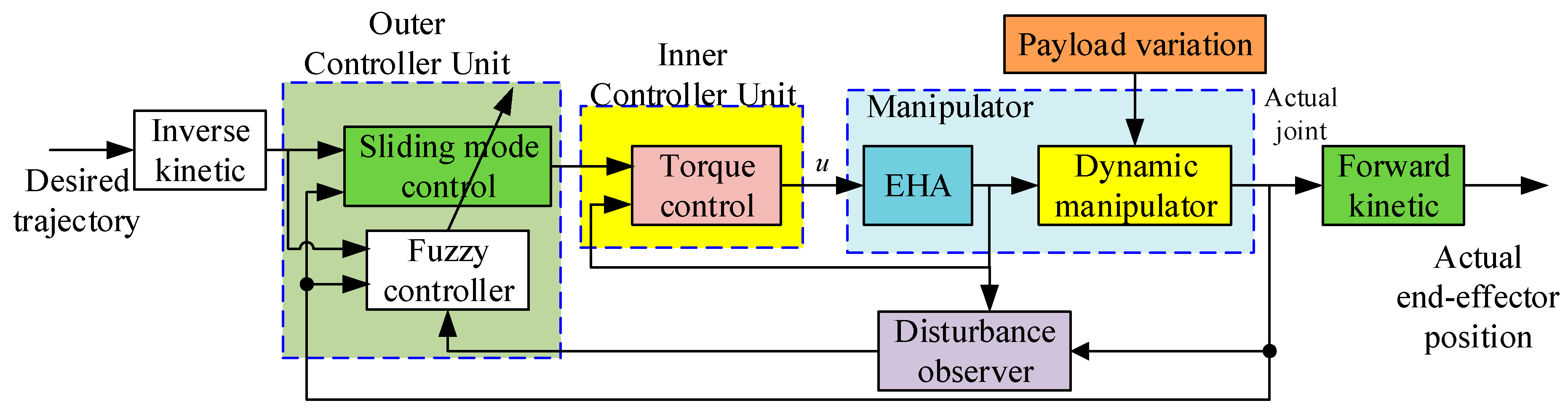
3. Adaptive Fuzzy Controller for the Hydraulic Manipulator

3.1. Cascade Control

In this paper, the proposed control is divided into two subsystems based on cascade control. In the outer loop, sliding mode control is employed to cope with the manipulator dynamic and generate desired torque for the hydraulic actuator, whereas the inner loop control using non-linear PI is utilized to run the actual torque induced by the EHA under the presence of the uncertainties and the highly nonlinear terms. The overview of the proposed control is illustrated in Figure 4.

Step 1: The sliding mode control for the manipulator dynamics.

Definite state variable errors $e=x_1-x_1{}_d\in R^{3\times 1}$, $\dot{e}=x_2-x_2{}_d\in R^{3\times 1}$, and $\ddot{e}={\dot{x}}_2-{\dot{x}}_{2d}\in R^{3\times 1}$, where $x_1{}_d\hspace{0.17em}\mathrm{and}\hspace{0.17em}{x}_{2d}\in R^{3\times 1}$ are the desired angular position and velocity, respectively. The sliding variable vector $s_1={\left[\begin{array}{ccc}{s}_{11}& s_{12}& s_{13}\end{array}\right]}^T\in R^{3\times 1}$ is chosen as follows:

$$s_1=\dot{e}+\lambda e$$

(17)

where $\lambda =diag\left({\lambda }_1,\dots ,{\lambda }_3\right)$ is a positive-definite matrix.

The reference state of the manipulator is defined as:

$$\{\begin{array}{l}{x}_2{}_s=x_2-s_1=x_2{}_d-\lambda e\in R^{3\times 1}\\ {\dot{x}}_{2s}={\dot{x}}_2-{\dot{s}}_1={\dot{x}}_{2d}-\lambda \dot{e}\in R^{3\times 1}\end{array}$$

(18)

The derivative of the sliding variable with respect to time is expressed as follows:

$${\dot{s}}_1=\ddot{e}+\lambda \dot{e}$$

(19)

Replacing (17), (18), and (19) into the 2nd equation of (16) yields:

$$M_0\left(q\right){\dot{s}}_1=J\left(x_1\right)x_3-{\Delta }_1\left(t\right)-M_0\left(x_1\right){\dot{x}}_{2s}-C_0\left(x_1,x_2\right)x_{2s}-G_0\left(x_1\right)-\frac{1}{2}{\dot{M}}_0\left(x_1\right)s_1$$

(20)

The desired torques are chosen as follows:

$$x_{3d}=J{\left(x_1\right)}^{-1}(C_0\left(x_1,x_2\right)x_{2s}+G_0\left(x_1\right)+M_0\left(x_1\right){\dot{x}}_{2s}-K_1{s}_1-\eta \mathrm{si}gn\left(s_1\right))$$

(21)

The reaching law is designed as:

$$\dot{s}=-K_1{s}_1-\eta \mathrm{si}gn\left(s_1\right)$$

(22)

where $K_1=diag\left(k_{11},\dots ,k_{13}\right)\in R^{3\times 3}$ is the positive definite matrix, ${\eta }_1=diag\left({\eta }_{11},\dots ,{\eta }_{13}\right)\in R^{3\times 3}$ is the positive definite matrix, it is chosen how to ${\eta }_{1i}\ge \left|{\Delta }_{1i}\left(t\right)\right|\left(i=1,\dots ,3\right)$. By adding the proportional rate term $-K_1{s}_1$, the state is forced to approach the switching manifolds faster when $s_1$ is large. The sign function is defined by:

$$\begin{array}{l}sign\left(s_1\right)={\left[\begin{array}{ccc}sign\left(s_{11}\right)& sign\left(s_{12}\right)& sign\left(s_{13}\right)\end{array}\right]}^T\\ sign\left(s_{1i}\right)=\{\begin{array}{cc}1& if\hspace{0.17em}{s}_{1i}\left(t\right)\ge 0\\ -1& if\hspace{0.17em}{s}_{1i}\left(t\right)<0\end{array}\end{array}$$

(23)

Define the torque error vector

$$s_2=x_3-x_{3d}$$

(24)

with $s_2={\left[\begin{array}{ccc}{s}_{21}& s_{22}& s_{23}\end{array}\right]}^T\in R^{3\times 1}$.

To prove the stability and robustness of the manipulator, the Lyapunov candidate function is chosen as follows:

$$V_1\left(s_1\right)=\frac{1}{2}{s}_1{}^T{M}_0{s}_1$$

(25)

The derivative of the Lyapunov functions is presented as follows:

$${\dot{V}}_1\left(s_1\right)=s_1{}^T{M}_0{\dot{s}}_1+\frac{1}{2}{s}_1{}^T{\dot{M}}_0{s}_1$$

(26)

Putting the Equations (21), (24), and (25) into Equation (26) can yield to:

$${\dot{V}}_1\left(s_1\right)=s_1{}^T{s}_2-s_1{}^T{K}_1{s}_1+s_1{}^T\left({\Delta }_1\left(t\right)-{\eta }_1\mathrm{si}gn\left(s_1\right)\right)$$

(27)

The sliding variable, s₁, will converge to zero when the derivative of the Lyapunov function is a negative semi-definite function. To satisfy this condition, a robust control for the hydraulic dynamic is developed to guarantee that the torque error, s₂, is bounded by $\epsilon$.

Step 2: Designing the control, to guarantee the torque error is as small as possible. The differential of the torque error is derived as:

$${\dot{s}}_2={\dot{x}}_3-{\dot{x}}_{3d}=-F_1\left(x\right)+F_2\left(x\right)U+{\Delta }_2\left(t\right)-{\dot{x}}_{3d}$$

(28)

The control vector is chosen as

$$U=F_2^{-1}(x)\left({\dot{x}}_{3d}-F_1(x)-K_2{s}_2-\Gamma {\upsilon }_2-s_1-{\eta }_{2}sign(s_2)\right)$$

(29)

where $K_2=diag\left(k_{21},k_{22},k_{23}\right)$ and $\Gamma =diag\left({\gamma }_1,{\gamma }_2,{\gamma }_3\right)$ are arbitrary positive matrices, ${\upsilon }_2={\displaystyle {\int }_0^t{s}_2\left(\tau \right)d\tau }\in R^{3\times 1}$, ${\eta }_2=diag\left({\eta }_{21},\dots ,{\eta }_{23}\right)\in R^{3\times 3}$ is a robust gain diagonal positive $d_2$ matrix of the sliding mode control s₂, and the sign function $\mathrm{sgn}\left(s_2\right)$ is defined by:

$$\begin{array}{l}sign\left(s_2\right)={\left[\begin{array}{ccc}sign\left(s_{21}\right)& sign\left(s_{22}\right)& sign\left(s_{23}\right)\end{array}\right]}^T\\ sign\left(s_{2i}\right)=\{\begin{array}{cc}1& if\hspace{0.17em}{s}_{2i}\left(t\right)\ge 0\\ -1& if\hspace{0.17em}{s}_{2i}\left(t\right)<0\end{array}\end{array}$$

(30)

Assumption 2.

The perturbation,${\Delta }_2\left(t\right)$, varies with respect to time, and it is bounded$\Vert {\Delta }_{2i}\left(t\right)\Vert \le {\eta }_{2i}\left(i=1,\dots ,3\right)$.

Considering the Lyapunov function candidate:

$$V_2\left(s_1,s_2\right)=V_1\left(s_1\right)+\frac{1}{2}{s}_2^T{s}_2+\frac{1}{2}{\upsilon }_2^T\Gamma {\upsilon }_2$$

(31)

The derivative of the Lyapunov function (31) is:

$${\dot{V}}_2\left(s_1,s_2\right)={\dot{V}}_1\left(s_1\right)+s_2^T\left({\dot{s}}_2\left(t\right)+\Gamma {\upsilon }_2\right)$$

(32)

Replacing (29) and (27) into (32), the derivative of the Lyapunov function can be rewritten as follows:

$${\dot{V}}_2\left(s_1,s_2\right)={\dot{V}}_1\left(s_1\right)+s_2^T\left({\dot{s}}_2\left(t\right)+\Gamma {\upsilon }_2\right)\le {\displaystyle \sum _{i=1}^2-s_i^T{K}_i{s}_i+s_i{}^T\left({\Delta }_i\left(t\right)-{\eta }_i\mathrm{si}gn\left(s_i\right)\right)}\le {\displaystyle \sum _{i=1}^2-s_i^T{K}_i{s}_i}$$

(33)

As shown in (33), ${\dot{V}}_2\left(s_1\left(t\right),s_2\left(t\right)\right)$ is a negative-definite function, $V_2\left(s_1\left(t\right),s_2\left(t\right)\right)\le V_2\left(s_1\left(0\right),s_2\left(0\right)\right)$. It means that s₁ and s₂ are bounded. Let function $P_{v2}=s_1^T{K}_1{s}_1+s_2^T{K}_2{s}_2\le -{\dot{V}}_2$ and integrate function $P_{v2}$ with respect to time.

$${\displaystyle \underset{0}{\overset{t}{\int }}{P}_{v2}\left(\tau \right)d\tau }\le V_2\left(s_1\left(0\right),s_2\left(0\right)\right)-V_2\left(s_1\left(t\right),s_2\left(t\right)\right)$$

(34)

Because $V_2\left(s_1\left(0\right),s_2\left(0\right)\right)$ is a bounded function, and $V_2\left(s_1\left(t\right),s_2\left(t\right)\right)$ is nonincreasing and bounded, so:

$$\underset{t\to \infty }{\lim }{\displaystyle \underset{0}{\overset{t}{\int }}{P}_{v2}\left(\tau \right)d\tau }<\infty$$

(35)

Additionally, ${\dot{P}}_{v2}$ is also bounded, by Barbalat’s lemma [51], it can be shown that $\underset{t\to \infty }{\lim }{\displaystyle \underset{0}{\overset{t}{\int }}{P}_{V2}\left(\tau \right)d\tau =0}$ and the sliding variable constants are chosen to satisfy the Hurwitz theorem. They mean that the vector $s_1\left(t\right)$, $s_2\left(t\right)$, $e_1\left(t\right)$ and $e_2\left(t\right)$ will converge to zero as $t\to \infty$.

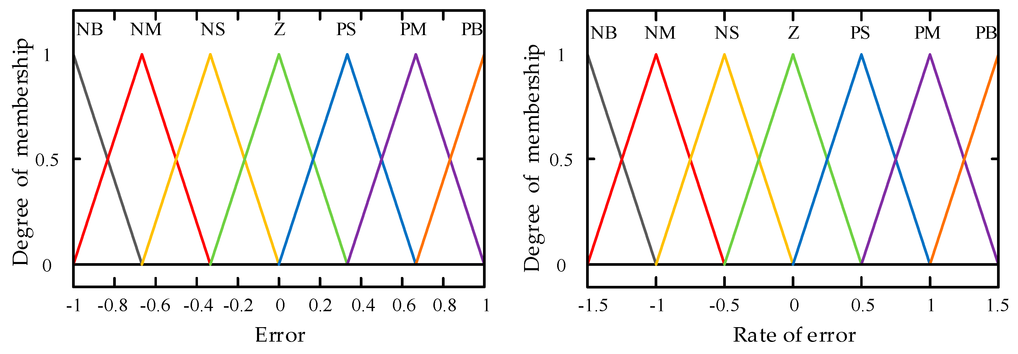
3.2. Adaptive Fuzzy Logic System

In practice, the manipulator works under the presence of payload variation, uncertainties, or unmodeled parameters that affect the dynamic manipulator. The controller normally is structured so that the manipulator can work stably within a permissible range. Out of this range, the system is unstable. This issue can be solved by using the high gain method with the large value of feedback gains which will cover the range of the uncertainties. In this way, for instance, disturbances or noise is amplified as well, or the chattering phenomenon appears [52] that make robot oscillate during the working process, degrades the performance of the system, and may lead to instability. Then to obtain accurate tracking performance and satisfy the work condition, the fuzzy logic control whose rules depended on the control objective is designed. First, to reflect the effect of the payload, let us rewrite the Equation (21):

$$x_{3d}=J{\left(x_1\right)}^{-1}(C_0\left(x_1,x_2\right)x_{2s}+G_0\left(x_1\right)+M_0\left(x_1\right){\dot{x}}_{2s}-K_1^{*}{s}_1-\eta \mathrm{sign}\left(s_1\right))$$

(36)

where $K_1^{*}=K_1+K_m$, and K_m are the positive definite matrices. $K_1\hspace{0.17em}\mathrm{and}\hspace{0.17em}\eta$ are adjusted based on the motion of the tracking error and its changing rate whereas K_m is directly depended on the payload attached at the end-effector so that the control signal can adopt the performance.

The linguistic fuzzy rules are defined in the following form:

$$\begin{array}{c}\mathrm{IF} e(t)\hspace{0.17em}\mathrm{is}\hspace{0.17em}{A}_1^{i=1,2,\dots ,N}\hspace{0.17em}\mathrm{and} \dot{e}(t)\hspace{0.17em}\mathrm{is}\hspace{0.17em}{A}_2^{i=1,2,\dots ,N}\\ \mathrm{THEN} K \mathrm{is} B^{i=1,2,\dots ,N}.\end{array}$$

(37)

where N is the total number of rules, K represents for the tuned gains feedback, $A_{1,2}^i\hspace{0.17em}\mathrm{and}\hspace{0.17em}{B}^i$ are the linguistic variables of the fuzzy sets characterized by fuzzy membership functions. The fuzzy control rules can be represented as the mapping of the input linguistic variables e(t) and $\dot{e}(t)$ to the output linguistic variable K. The input linguistic variable characterized by seven membership functions (NB (Negative Big), NM (Negative Medium), NS (Negative Small), Z (Zero), PS (Positive Small), PM (Positive Medium), PB (Positive Big)) are employed for the control strategy such that the stability of the system can be guaranteed as stable. The membership functions of the two input linguistic variables $e(t)\hspace{0.17em}\mathrm{and}\hspace{0.17em}\dot{e}(t)$ and the output linguistic variable K are described in Figure 5 and Figure 6, (VVS (Very Very Small), VS (Very Small), S (Small), M (Medium), B (Big), VB (Very Big), VVB (Very Very Big)); the control strategy is described in

Table 1. Rules table of the fuzzy logic system.

${\mathit{K}}_1$		$\dot{\mathit{e}}(\mathit{t})$
		NB	NM	NS	Z	PS	PM	PB
e(t)	NB	M	B	VB	VVB	VB	B	M
	NM	S	M	B	VB	B	M	S
	NS	VS	S	M	B	M	S	VS
	Z	VVS	VS	S	M	S	VS	VVS
	PS	VS	S	M	B	M	S	VS
	PM	S	M	B	VB	B	M	S
	PB	M	B	VB	VVB	VB	B	M

[38]. In this study, triangular membership functions are considered as shown in Figure 5 and Figure 6. The value of η is calculated as:

$$\eta =K_1/1000$$

(38)

The second part of the fuzzy logic system is attached for adjusting gain to satisfy the changing of the payload. Based on the change in acceleration because of a sudden change in inertia, the torque induced on each link is changed, thus leading to the variation in the state error. Then, the scaling gains affected by the load torque is designed to adapt to the system working operation.

$$K_m=Fuzzy(\mathrm{payload})$$

(39)

Under the presence of the external load, the compensated torque generated by the secondary fuzzy logic system is attached to boost the control signal. In this research, we consider that the external payload attached to the end-effector will beget the external torque. The force then is identified by using a non-linear disturbance observer [41,42]. Then we suggest a method to estimate the external payload for the compensator. In such a way that the trackability issue incurred from loading external mass is improved. The mass of the payload is assumed to be distributed in the interval from 4 to 50 kg. Then the load torque is observed and added to compensate the control input signal. Seven membership functions namely NB (Negative Big), NM (Negative Medium), NS (Negative Small), Z (zero), PS (Positive Small), PM (Positive Medium), PB (Positive Big) are the linguistic input variables. For the output of the fuzzy system, the adjustable scaling gain K_m specified by seven membership functions including Z (Zero), S (Small), LS (Light Small), M (medium), LB (Light Big), B (Big), VB (Very Big) is employed. Both linguistic input and output sets are signified in detail in Figure 7 and Figure 8. The fuzzy rules are defined by IF-THEN rules and its laws are discussed in

Table 2. Rules table of the fuzzy logic system.

${\mathit{K}}_{\mathit{m}\mathit{i}}$		${\mathit{\tau }}_{\mathit{l}\mathit{o}\mathit{a}\mathit{d}\_\mathit{i}}$
		NB	NM	NS	Z	PS	PM	PB
${\tau }_{load\_j}$	NB	VB	B	LB	M	LB	B	VB
	NM	B	LB	M	LM	M	LB	B
	NS	LB	M	LM	S	LM	M	LB
	Z	M	LM	S	Z	S	LM	M
	PS	LB	M	LM	S	LM	M	LB
	PM	B	LB	M	LM	M	LB	B
	PB	VB	B	LB	M	LB	B	VB

. The triangular membership functions are described in Figure 7 for the change of load torque and Figure 8 for the adaptive gains.

$$\begin{array}{c}\mathrm{IF} T_{load\_i}\hspace{0.17em}\mathrm{is}\hspace{0.17em}{A}_1^{p=1,2,\dots ,N}\hspace{0.17em}\mathrm{and} T_{load\_j}\mathrm{is}\hspace{0.17em}{A}_2^{p=1,2,\dots ,N}\\ \mathrm{THEN}{K}_{mi}\hspace{0.17em}\hspace{0.17em}\mathrm{is}\hspace{0.17em}\hspace{0.17em}{K}_{payload}^{p=1,2,\dots ,N}\end{array}$$

(40)

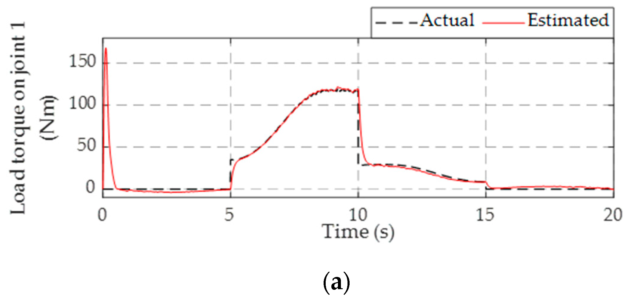
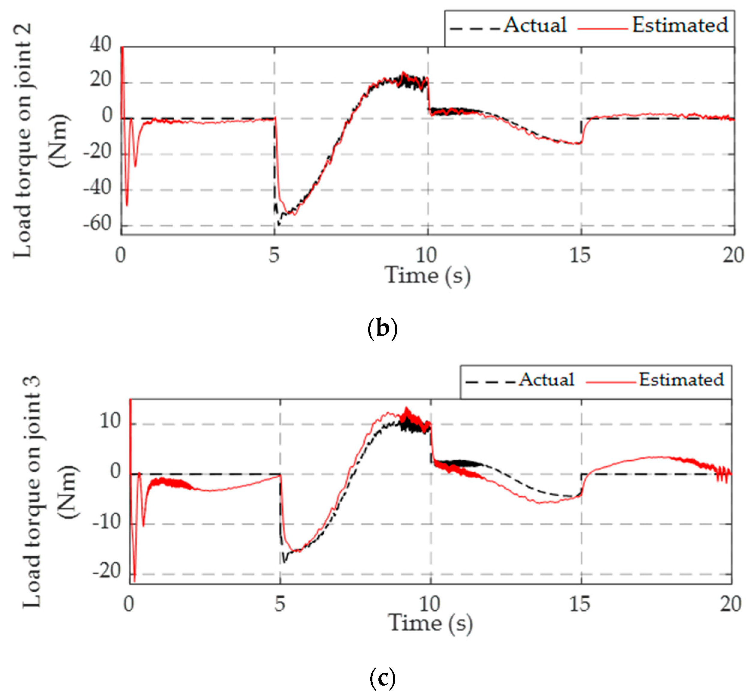
3.3. Nonlinear Disturbance Observer

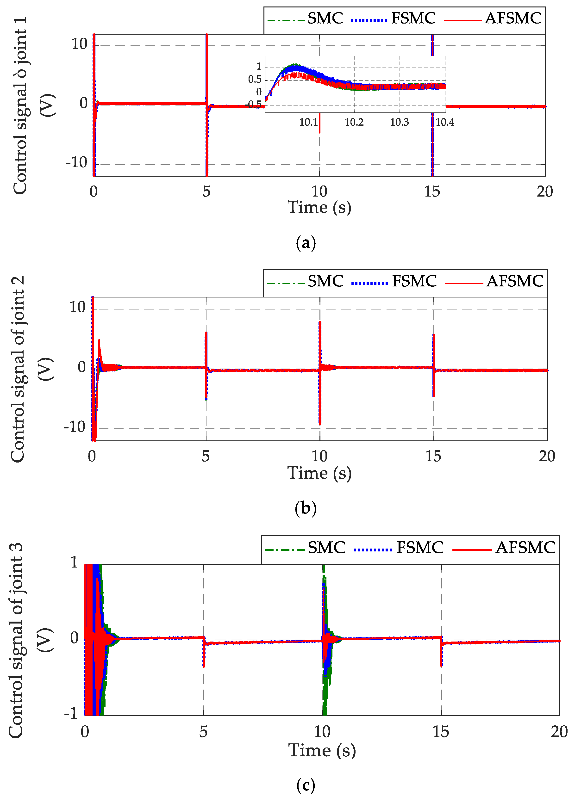
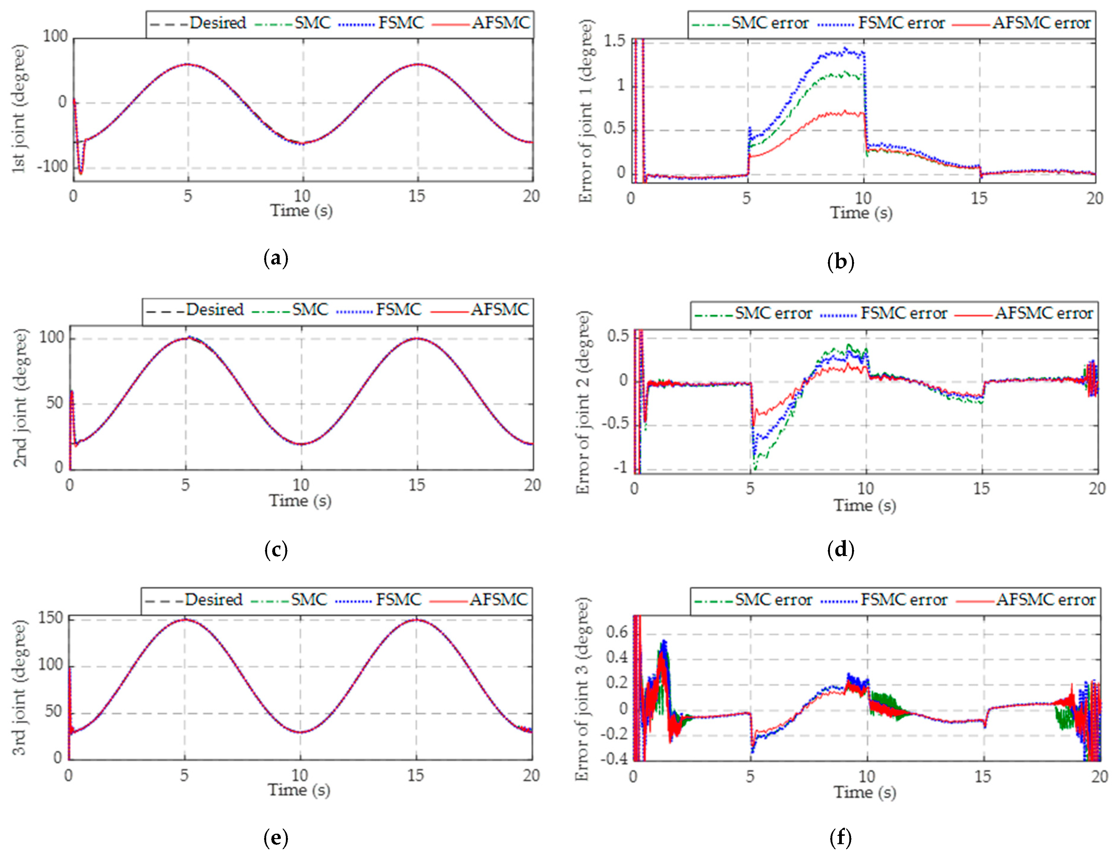
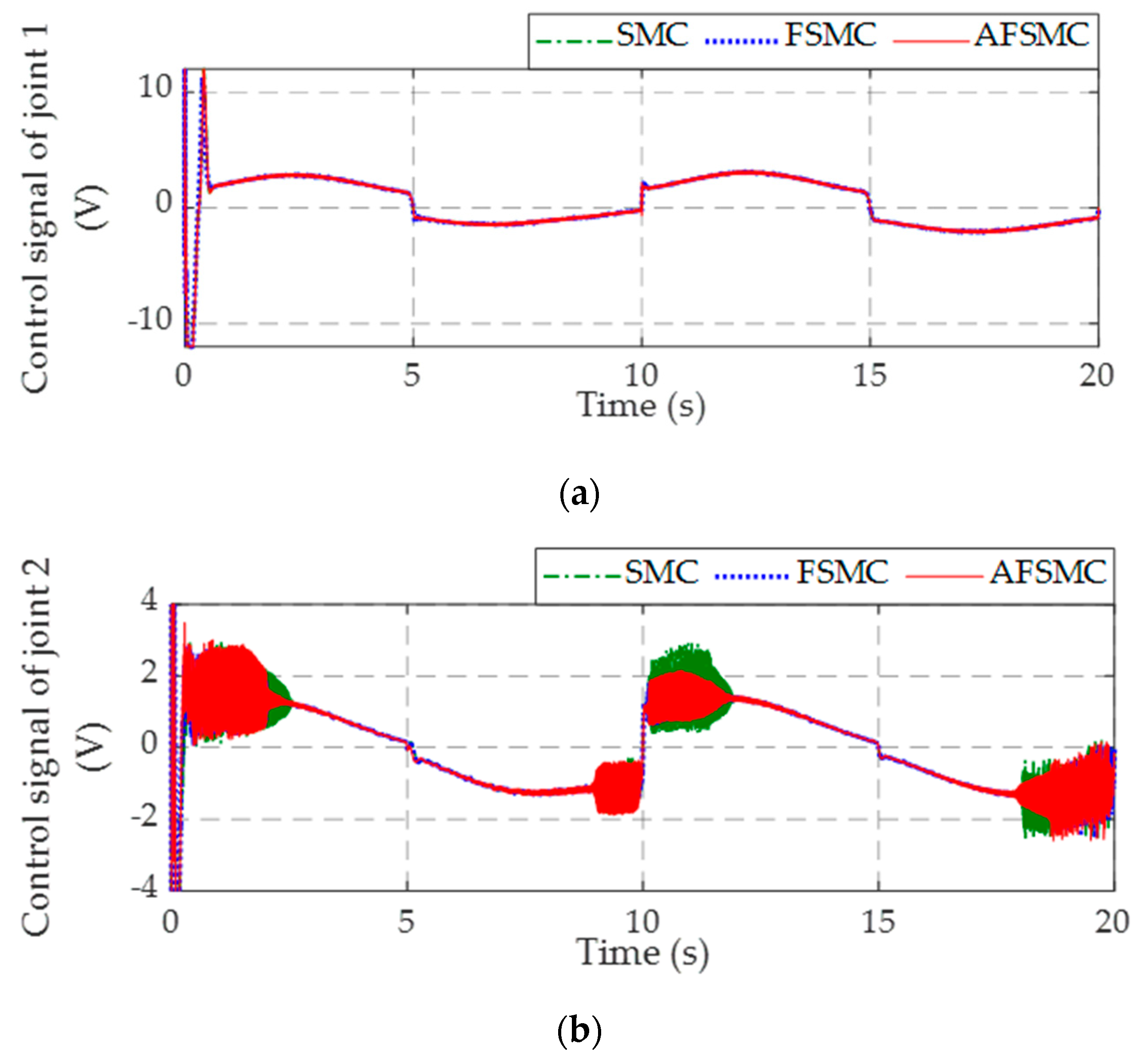
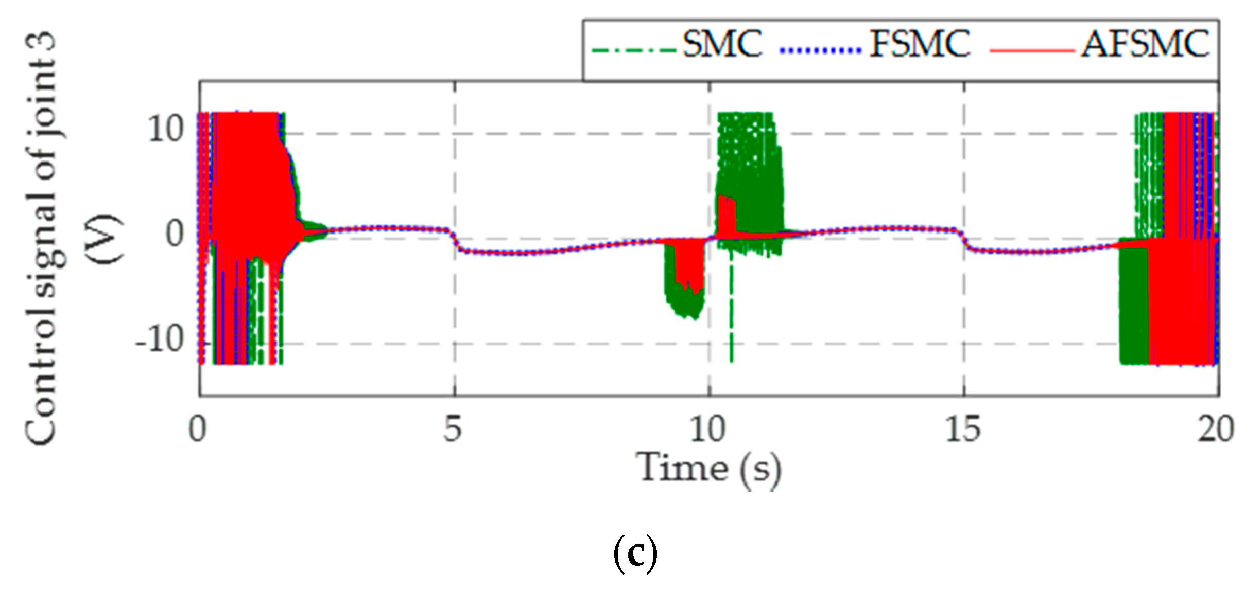
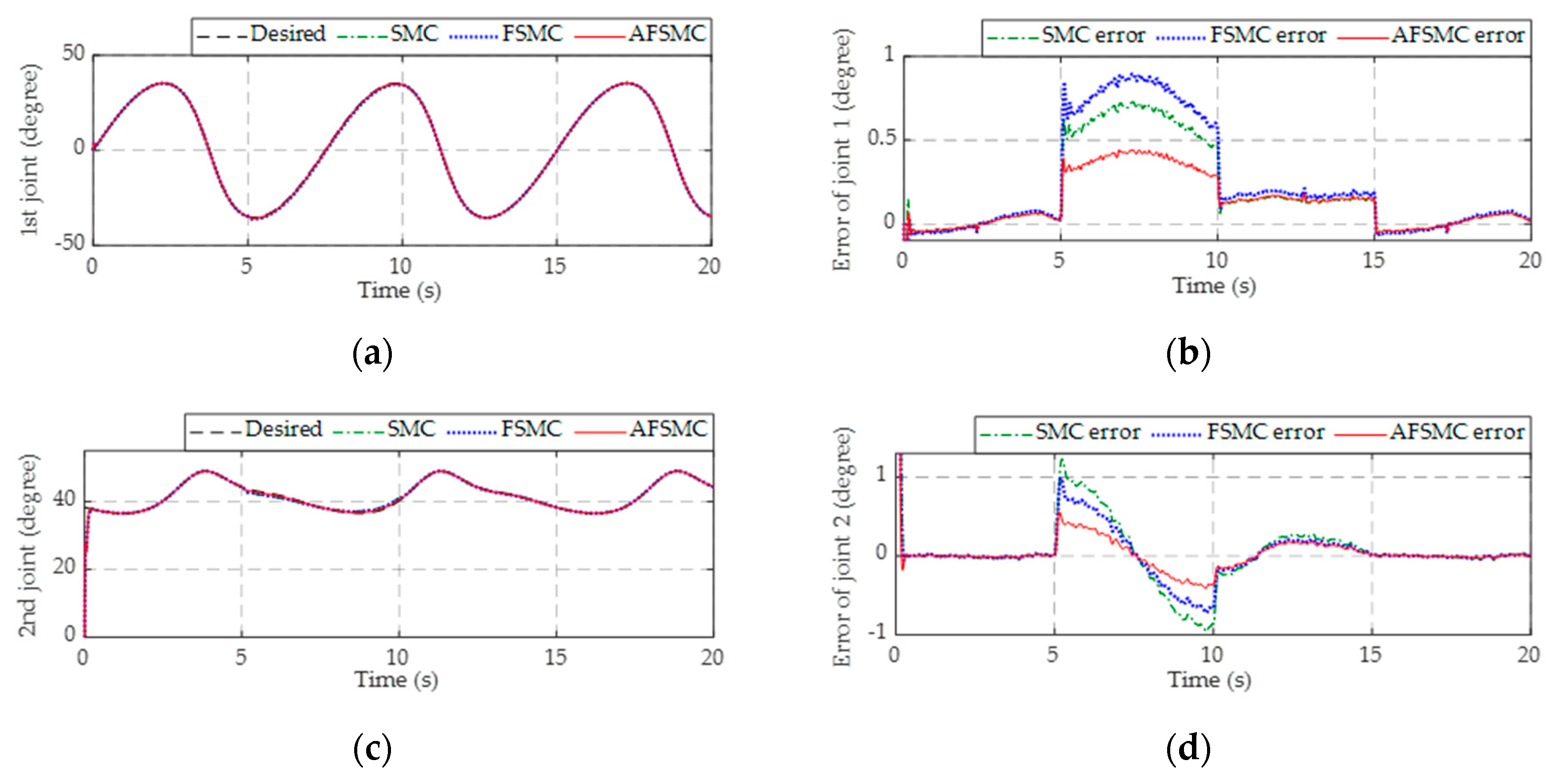
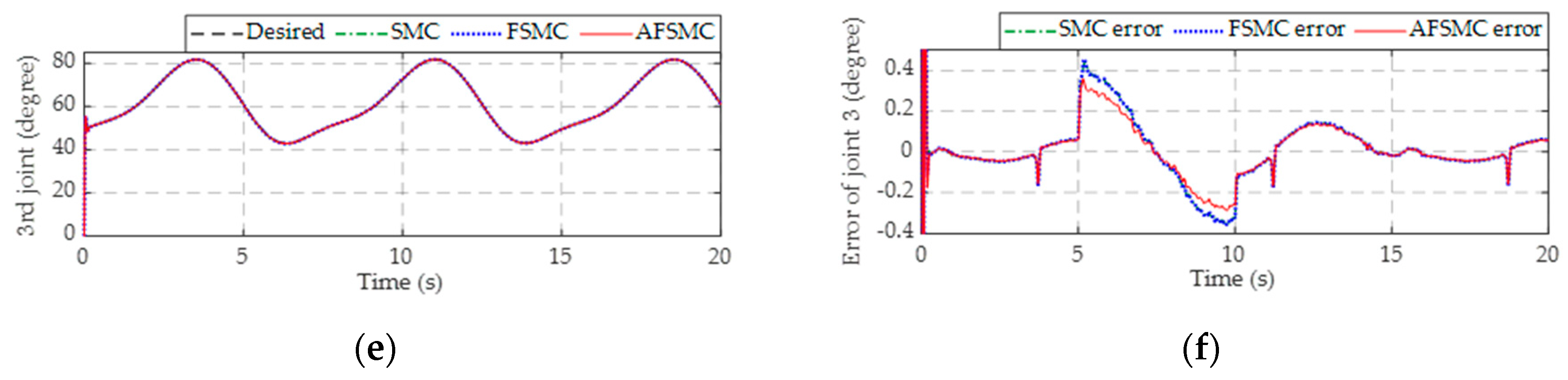
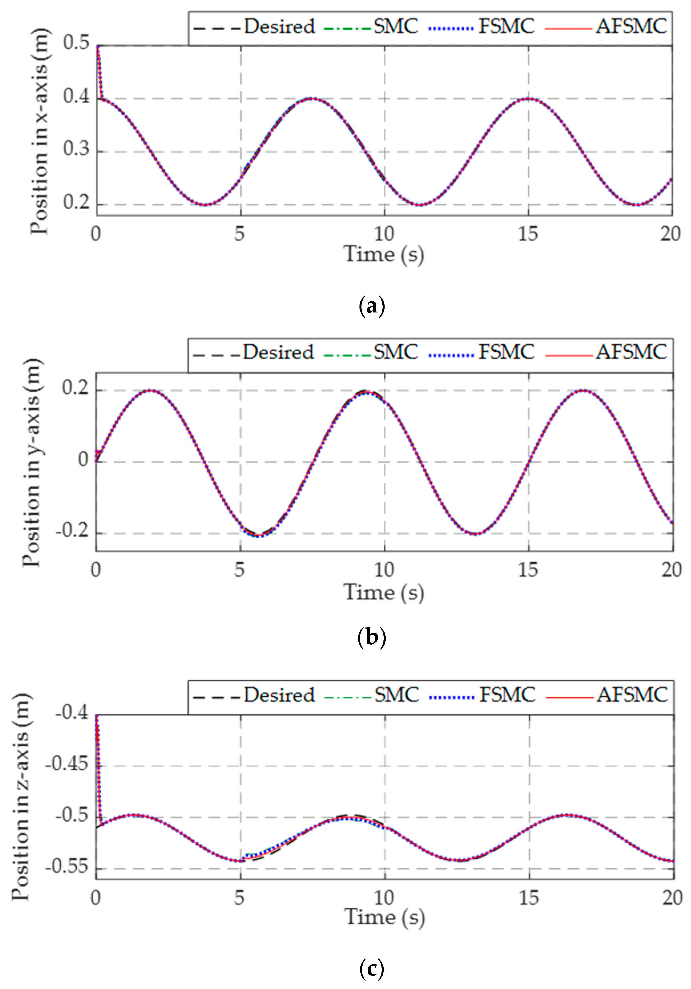
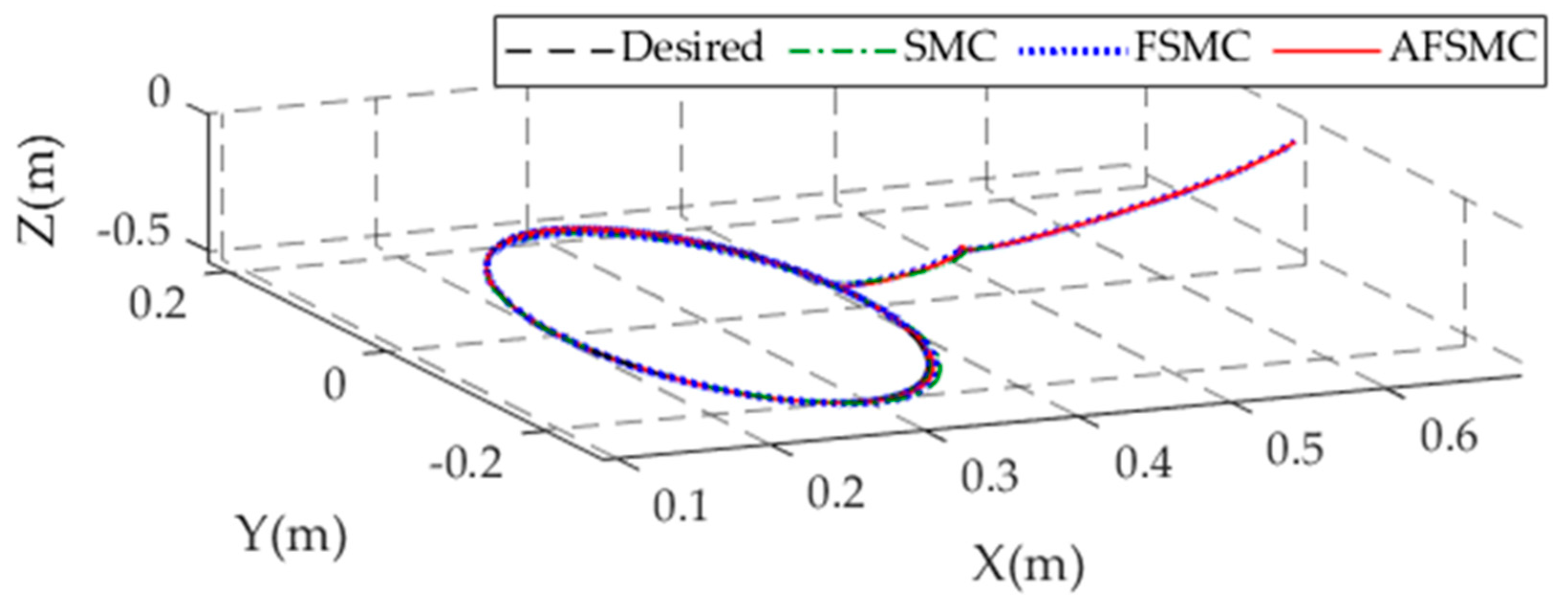
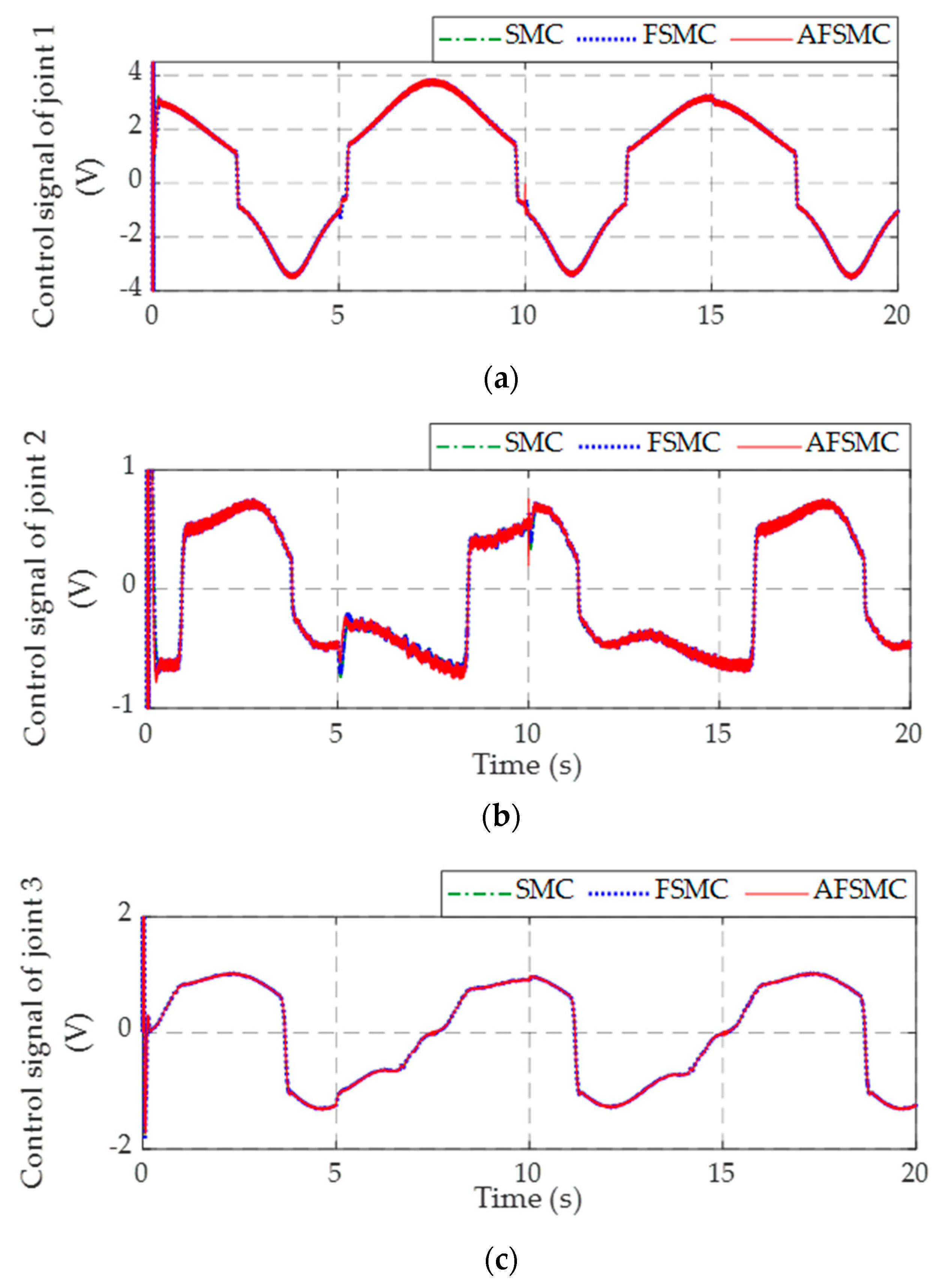
The disturbance observer (DO) is normally used to estimate and eliminate the effect of external disturbance from the environment or some internal disturbance insider the system such as friction. The advantages of the disturbance observer are briefly shown in [41,42]. In this study, the DO is used to observe the change of the external payload considered as an external disturbance.

Since the external disturbance cannot be measured, hence according to [15], this estimated parameter is computed by:

$$\widehat{d}=z+p\left(q,\dot{q}\right)$$

(41)

where $\widehat{d}\in R^{3\times 1}$ is an estimated disturbance, z$\in R^{3\times 1}$ is an auxiliary variable used to cancel out an acceleration measurement in the term $M\left(q\right)\ddot{q}$, function p is chosen as:

$$p\left(q,\dot{q}\right)=\alpha \left(\begin{array}{ccc}1& 0& 0\\ 1& 1& 0\\ 1& 1& 1\end{array}\right)\ddot{q}$$

(42)

where α is a constant depending on the maximum velocity of the third link.

The auxiliary variable z can be obtained from:

$$\dot{z}=-L(q,\dot{q})z+L(q,\dot{q})\left\{C\left(q,\dot{q}\right)+G\left(q\right)-\tau -p\left(q,\dot{q}\right)\right\}$$

(43)

where

$$L(q,\dot{q})=\frac{d}{dt}\left(p(q,\dot{q})\right)M{(q)}^{-1}{\ddot{q}}^{-1}=\alpha \left(\begin{array}{ccc}1& 0& 0\\ 1& 1& 0\\ 1& 1& 1\end{array}\right)M{(q)}^{-1}$$

(44)

The proof of the stability of the DO can be deduced from [42].

4. Simulations

In this part, some numerical simulations and comparison are implemented to evaluate the effectiveness of the proposed algorithm by using the MATLAB/Simulink program. The mechanical parameters and hydraulic parameters used for simulating are shown in

Table 3. The mechanical parameters used for simulations.

Parameter	Value (unit)
$m_1$	5 (kg)
$m_2$	5 (kg)
$m_3$	5 (kg)
$l_1$	0.3 (m)
$l_2$	0.5 (m)
$l_3$	0.2 (m)
g	9.81 (m/s2)

and

Table 4. The hydraulic parameters used for simulations.

Parameter	Value (Unit)
$A_{ij}{}_{\left(i,j=1,2\right)}$	1.15 $\times$ 10−4 (m3/rad)
$A_{31}$	${0.0442}^2\pi /4$ (m2)
$A_{32}$	$\pi ({0.0442}^2-{0.025}^2)/4$ (m2)
$\rho$	870 (kg/m3)
$P_S$	100 (bar)
$P_r$	2 (bar)
Effective Bulk modulus β	1.25 $\times$ 109 (Pa)

, respectively. In our simulations, discrete time with the fixed step is 10⁻⁴ s and the Runge–Kutta method is used for the approximate calculation of some differential problems. We investigate performance of the manipulator in three case studies with the same condition: the initial value of the three joints is ${[\begin{array}{ccc}0.1& 0.6& 0.8\end{array}]}^T$ (rad), and the initial velocity of the three joints are all zero; the external payload varies in the interval [5,20] kg and is shown in Figure 9; and the time for simulating is 20 s. The comparison between sliding mode control (SMC), fuzzy sliding mode control (FSMC), and adaptive fuzzy sliding mode control (AFSMC) are utilized. The white noise is added to illustrate uncertainty parameters and verify the proposed method.

The Controller gains used for simulation are $k_{qij}{}_{\left(i,j=1,2\right)}={2.1610}^{-8}{m}^3/\left(\sqrt{Pa}.s.V\right)$, λ = diag (60, 60, 50), $k_{qi3}{}_{\left(i=1,2\right)}={3.510}^{-8}{m}^3/\left(\sqrt{Pa}.s.V\right)$, $k_{21}={10}^3$, $k_{22}={10}^3$, $k_{23}={5.10}^4$, ${\gamma }_1={2.10}^6$, ${\gamma }_2={2.10}^6$, ${\gamma }_3={2.10}^7$, ${\eta }_{22}={10}^4$, and ${\eta }_{23}={10}^5$.

Case study 1: The desired trajectory of the three joints is supposed to be tooth saw profile created by input shaping. The desired trajectory of the three joints and the responses while using three methods are described in Figure 10. The role of the proposed controller is validated at the time when the external payload is applied. The error of the AFSMC is the smallest, in which the smallest overshoot is at the time the payload changed, compared with that of the FSMC and SMC. The load torques estimated by using disturbance observer are depicted in Figure 11. And the control input signals which are constrained in the interval [−15, 15] (V) are performed in Figure 12.

Case study 2: In this case, sine function signals are used as the desired performance. The three joints trajectory are designed as:

$$\{\begin{array}{ll}{q}_{1d}=60\sin \left(\raisebox{1ex}{$\pi t$}\!\left/ \!\raisebox{-1ex}{$5$}\right.-\raisebox{1ex}{$\pi $}\!\left/ \!\raisebox{-1ex}{$2$}\right.\right)& (\mathrm{degree})\\ q_{2d}=40\sin \left(\raisebox{1ex}{$\pi t$}\!\left/ \!\raisebox{-1ex}{$5$}\right.-\raisebox{1ex}{$\pi $}\!\left/ \!\raisebox{-1ex}{$2$}\right.\right)+60& (\mathrm{degree})\\ q_{3d}=60\sin \left(\raisebox{1ex}{$\pi t$}\!\left/ \!\raisebox{-1ex}{$5$}\right.-\raisebox{1ex}{$\pi $}\!\left/ \!\raisebox{-1ex}{$2$}\right.\right)+90& (\mathrm{degree})\end{array}$$

(45)

In this case study, the sinusoidal signals are used as a smooth function to investigate the feedback states. The tracking performance of the three joints are described in Figure 13, the load torques estimated are depicted in Figure 14 and the control input signals are depicted in Figure 15. As can be seen in Figure 14, no matter how changed the load torques is, the DO can estimate its change for the compensation.

Case study 3: This last simulation is implemented in task space (Cartesian co-ordinate). The end-effector is controlled to track the ellipse curve. The desired trajectory based on the working space of the robot in 3D space is supposed to be:

$$P=\left(\begin{array}{c}{P}_x\\ P_y\\ P_z\end{array}\right)=\left(\begin{array}{c}0.3+0.1\sin \left(\pi t/5\right)\\ 0.2\sin \left(\pi t/5\right)\\ -0.55+0.1\left(P_x+P_y\right)\end{array}\right)(m)$$

(46)

The Jacobian matrix is expressed in Appendix B. The responses of the end-effector in 3D space and the responses of the three joints are described in Figure 16, the movement of the end-effector in x, y, and z directions are depicted in Figure 17 and the behavior of the end-effector in Cartesian space in shown in Figure 18. The load torques estimated are depicted in Figure 19 and Figure 20 shows the control input signals of the three joints.

In the three case studies, the payload suddenly changes to 20 kg at the 5th second and drops to 5 kg and zero at the 10th and 15th second, respectively. The change of the payload results in changing in the external loads torque. As can be seen in Figure 11, Figure 14, and Figure 19 corresponding to the three case studies, the torques load can be observed and its profile correspond to that of the payload. The observed torques load of the second joint are similar to that of the third joint because of the same motion in the space. Owing to the fuzzy rules described in Table 2, the observed torques load can track the actual one, thus calculating and compensating the control signals. Herein only the magnitude of the torques load is considered because neither of the values of torques load are negative or positive, they all affect the tracking performance of the system. With the adaptive law for torques load compensation, the AFSMC can exhibit and achieve the best performance in comparison with conventional SMC and FSMC. The conventional sliding mode scheme can adopt the robustness; however, the trackability is degraded due to the changing parameters affecting indirectly the manipulator dynamics. When applying the fuzzy logic system, the control signals can be partially compensated, and with the use of compensator inherited from using disturbance observer (DO), the exerted torques load have been observed and the trackability is improved significantly.

5. Experiments

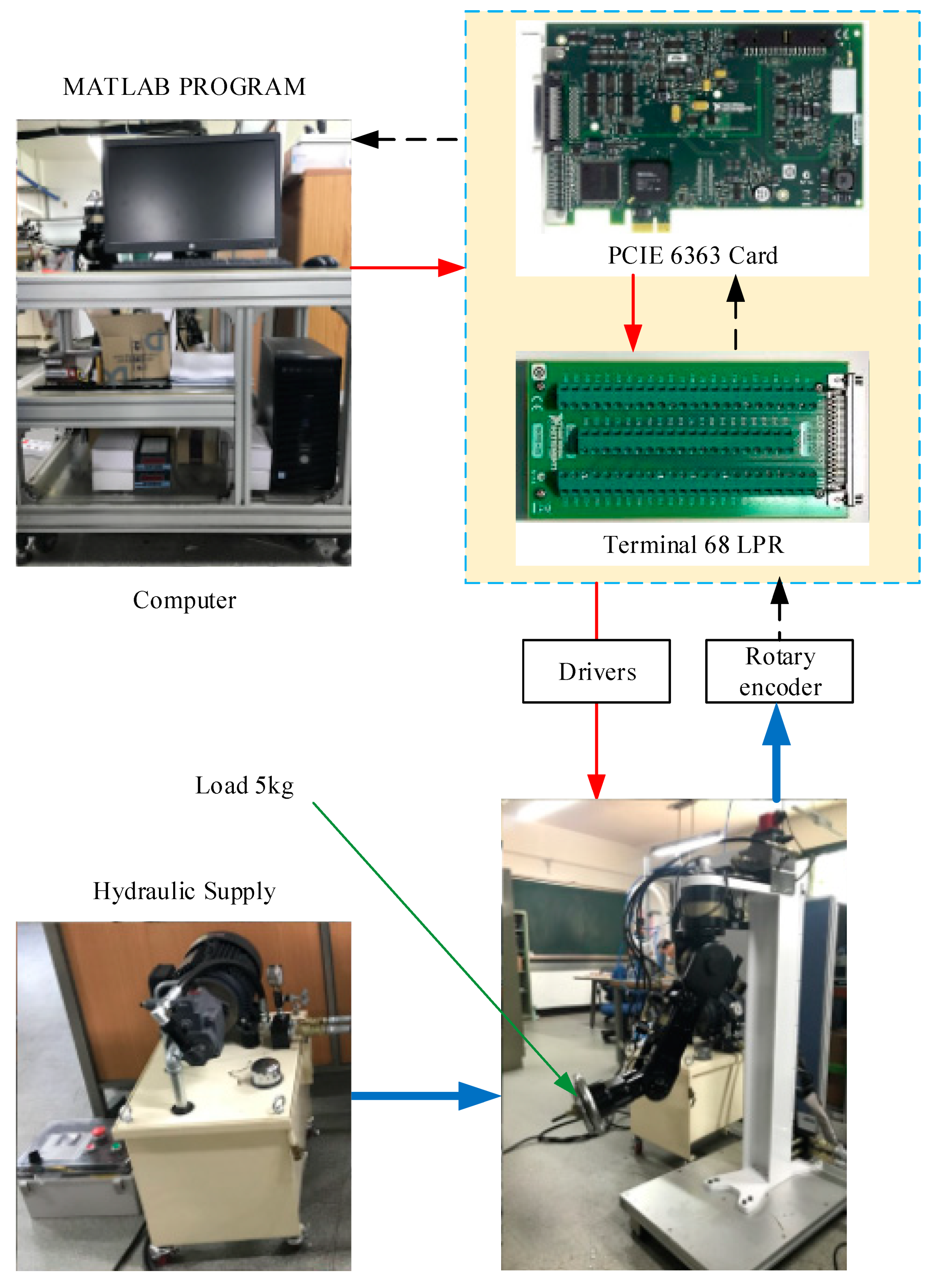
5.1. Experimental Setup

To verify and compare with the simulation, the proposed algorithm is applied on the real 3-DOF hydraulic manipulator. The hardware connection is depicted in Figure 21. The dash lines stand for the data derived from the system, and the solid lines stand for the command signal from the computer. The hardware setup includes the computer (PC) for data processing, the hydraulic supply for the manipulator, and the 3-DOF hydraulic manipulator communicating with the PC via terminal 68 LPR and the PCIE Card (PCIE-6363). The hydraulic manipulator supplied by the hydraulic system is driven by electro-hydraulic actuators equipped with incremental rotary encoders E40H6-5000-3-V-5 to measure the movement. The data read from encoders is then processed by the MATLAB program via PCIE card. After processing, the command signal from the computer is sent to the system to drive the servo valve amplifier SVA-R-1, thus generating the manipulator to follow the desired trajectory.

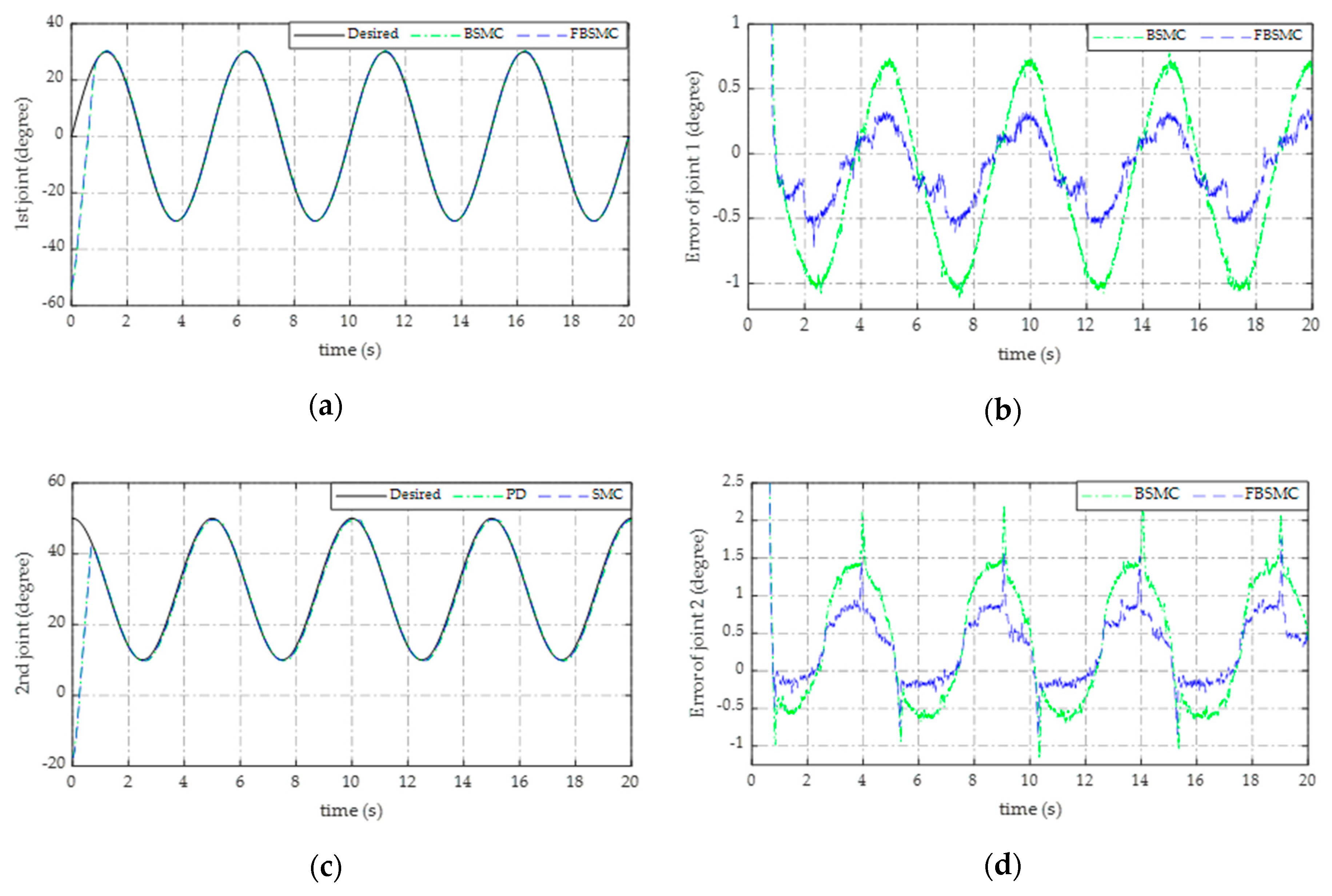
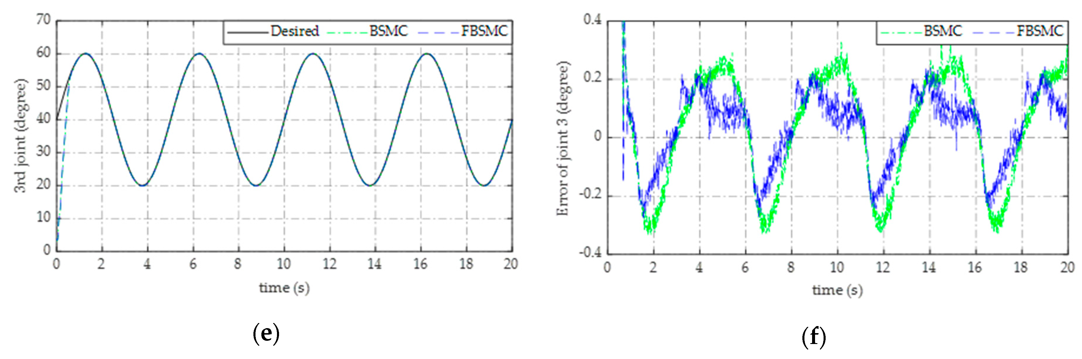
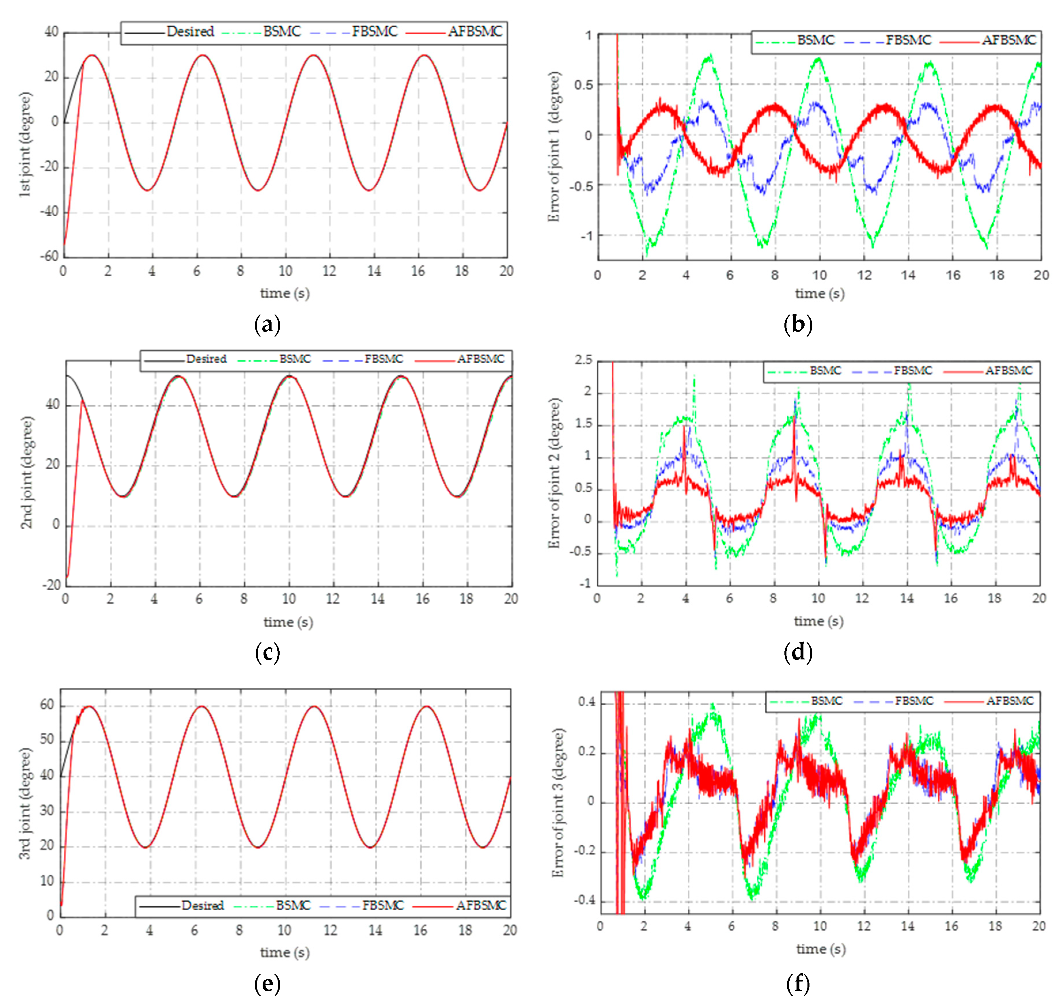
5.2. Experiment Results

In the experiments, we consider three case studies. The parameters of the system are same as defined in Table 3 and Table 4. The initial of the three joints is set when the actuators reaches the limited position (maximum extend for cylinder and maximum angular position for rotary actuators). The parameter of the sliding surface mentioned in Equation (17) is λ = diag (35, 30, 25), and the parameters of the robust terms in Equation (21) are $K_1=diag\left(40,40,40\right)$ and η = diag (1.8, 1.8, 1). The values of K₁ and η are different from the simulation because the real system has many uncertainties because of its structure and the different drivers used to run the manipulator, the gain is scheduled such that the system can operate smoothly. All the controller gains are kept same in the three case studies.

Case study 1: Sinusoidal signal and no load verification.

The desired trajectory is set as:

$$\{\begin{array}{ll}{q}_{1d}=30\sin \left(\raisebox{1ex}{$2\pi t$}\!\left/ \!\raisebox{-1ex}{$5$}\right.\right)& (\mathrm{degree})\\ q_{2d}=30+20\sin \left(\raisebox{1ex}{$2\pi t$}\!\left/ \!\raisebox{-1ex}{$5$}\right.+\raisebox{1ex}{$\pi $}\!\left/ \!\raisebox{-1ex}{$2$}\right.\right)& (\mathrm{degree})\\ q_{3d}=40+20\sin \left(\raisebox{1ex}{$2\pi t$}\!\left/ \!\raisebox{-1ex}{$5$}\right.\right)& (\mathrm{degree})\end{array}$$

(47)

In this case study, no load is attached into the end-effector. Therefore, the comparison is implemented between the conventional back-stepping slide ding mode control (BSMC) and fuzzy back-stepping sliding mode control (FBSMC). The response of the three joints is described in Figure 22.

Case study 2: The desired trajectory is set as same sinusoidal signal as the first case study, but 5 kg external payload is attached. The response of the three joints is depicted in Figure 23.

Case study 3: Step signal is applied instead of using smooth signal like the two above case studies or tooth saw profile like in the simulation. The controller parameters are still kept same as the original value setup above. The response of the system is shown in Figure 24.

As can be seen in the three case studies, depicted from Figure 22 to Figure 24, especially in the second and third case studies (Figure 23 and Figure 24), the response of the three joints is quite similar with the simulations, in which the errors when employing adaptive fuzzy back-stepping sliding mode control (AFBSMC) is the smallest compared with that of the fuzzy back-stepping sliding mode control (FBSMC) and back-stepping sliding mode control (BSMC). The error of the third joint in case of load and without load is quite similar. This can be explained as the short length of the third joint gets less affected from the load. But because of the length in the second link and dynamics coupling torque between the third and the second link, the error of the second joint is a little greater than that of when no load affected. When utilizing AFBSMC, the error decreased significantly. Same profile in the first joint in comparison between with and without load.

6. Conclusions

In this study, the behavior of the 3-DOF hydraulic manipulator including actuator has been analyzed. The tracking motion of the manipulator was investigated under the presence of the external payload. This main issue is handled by using adaptive fuzzy sliding mode control based on backstepping (BSP) control scheme. It employs the advantages of the SMC in reducing the order system, strong robustness against perturbation, and BSP control in solving both the problem of stabilization and tracking trajectory. The disturbance observer technique is employed to observe the change in the external torques induced by the variation of the external payload. Then the adaptive fuzzy logic scheme is used to adopt to the work condition. Some simulations and experiments have been given with the added noise and compared between the conventional backstepping sliding mode control, fuzzy back-stepping sliding mode control with the proposed algorithm to verify the robustness and stability of the algorithm in motion tracking. The results proved that the proposed control can improve the behavior of the 3-DOF hydraulic manipulator under the vastly changed payload, which occurs during operation in practice.

References

1. John, J.C. Introduction to Robotics Mechanics and Control, 3rd ed.; Addison-Wisley: Reading, PA, USA; Pearson Education Inc.: Upper Saddle River, NJ, USA, 1989. [Google Scholar]
2. Su, Y.X.; Muller, P.C.; Zheng, C.H. Global Asymptotic Saturated PID Control for Robot Manipulators. IEEE Trans. Control Syst. Technol. 2010, 18, 1280–1288. [Google Scholar] [CrossRef]
3. Li, S.; Ahmad, G.; Xie, W.; Gao, Y. An Enhanced IBVS Controller of a 6DOF Manipulator Using Hybrid PDSMC Method. Int. J. Control Autom. Syst. 2018, 16, 844–855. [Google Scholar] [CrossRef]
4. Nikdel, N.; Badamchizadeh, M.A.; Azimirad, V.; Nazari, M.A. Adaptive backstepping control for an n-degree of freedom robotic manipulator based on combined state augmentation. Robot. Comput. Integr. Manuf. 2017, 44, 129–143. [Google Scholar] [CrossRef]
5. Rong, J.W.; Rajkumar, M. Design of Fuzzy-Neural-Network-Inherited Backstepping Control for Robot Manipulator Including Actuator Dynamics. IEEE Trans. Fuzzy Syst. 2014, 22, 709–722. [Google Scholar]
6. Lee, H.S.; Won, S.J.; Ahn, K.K. The Numerical Modeling and Sliding Mode Control of a New Submersible Fish Cage. J. Drive Control 2017, 14, 18–24. [Google Scholar]
7. Baek, J.M.; Jin, M.L.; Han, S.H. A New Adaptive Sliding-Mode Control Scheme for Application to Robot Manipulators. IEEE Trans. Ind. Electron. 2016, 63, 3628–3637. [Google Scholar] [CrossRef]
8. Ha, T.W.; Jun, K.H.; Nguyen, M.T.; Han, S.M.; Shin, J.W.; Ahn, K.K. Position control of an Electro-Hydrostatic Rotary Actuator using adaptive PID control. J. Drive Control 2017, 14, 37–44. [Google Scholar]
9. Bo, Z.; Li, Y. Model-free Adaptive Dynamic Programming Based Near-optimal Decentralized Tracking Control of Reconfigurable Manipulators. Int. J. Control Autom. Syst. 2018, 16, 478–490. [Google Scholar]
10. Lv, W.S.; Wang, F.; Zhang, L.L. Adaptive Fuzzy Finite-time Control for Uncertain Nonlinear Systems with Dead-zone Input. Int. J. Control Autom. Syst. 2018, 16, 2549–2558. [Google Scholar] [CrossRef]
11. Ra, C.G.; Kim, S.K.; Suk, J.Y. Adaptive Sliding Mode Autopilot Design for Skid-to-turn Missile Model with Uncertainties. Int. J. Control Autom. Syst. 2017, 15, 2733–2743. [Google Scholar] [CrossRef]
12. To, X.D.; Ahn, K.K. Radial Basis Function Neural Network based Adaptive Fast Nonsingular Terminal Sliding Mode Controller for Piezo Positioning Stage. Int. J. Control Autom. Syst. 2017, 15, 2733–2743. [Google Scholar]
13. Vu, T.Y.; Wang, Y.N.; Pham, V.C.; Nguyen, X.Q.; Vu, H.T. Robust Adaptive Sliding Mode Control for Industrial Robot Manipulator Using Fuzzy Wavelet Neural Networks. Int. J. Control Autom. Syst. 2017, 15, 2930–2941. [Google Scholar]
14. Kim, M.; Kuc, T.Y.; Kim, H.; Lee, J.S. Adaptive Iterative Learning Controller with Input Learning Technique for a Class of Uncertain MIMO Nonlinear Systems. Int. J. Control Autom. Syst. 2017, 15, 315–328. [Google Scholar] [CrossRef]
15. Spong, M.W.; Seth, H.; Vidyasagar, M. Robot Dynamics and Control, 1st ed.; John Wiley & Sons, Inc.: New York, NY, USA, 2005. [Google Scholar]
16. Yuan, J. Adaptive control of robotic manipulators including motor dynamics. IEEE Trans. Robot. Autom. 1995, 11, 612–617. [Google Scholar] [CrossRef]
17. Tarn, T.J.; Bejczy, A.K.; Yun, X.; Li, Z. Effect of motor dynamics on nonlinear feedback robot arm control. IEEE Trans. Robot. Autom. 1991, 7, 114–122. [Google Scholar] [CrossRef]
18. Chen, B.S.; Uang, H.J.; Tseng, C.S. Robust tracking enhancement of robot systems including motor dynamics: A fuzzy-based dynamic game approach. IEEE Trans. Fuzzy Syst. 1998, 6, 538–552. [Google Scholar] [CrossRef]
19. Caldwell, D.G.; Medrano-Cerda, G.A.; Goodwin, M. Control of pneumatic muscle actuators. IEEE Control Syst. Mag. 1995, 15, 40–48. [Google Scholar]
20. Papoutsidakis, M.; Chatzopoulos, A.; Tseles, D. Hydraulics and Pneumatics: A Brief Summary of their Operational Characteristics. J. Multidiscip. Eng. Sci. Technol. 2018, 5, 8973–8977. [Google Scholar]
21. Chiag, C.J.; Chen, Y.C. Neural network fuzzy sliding mode control of pneumatic muscle actuators. Eng. Appl. Artif. Intell. 2017, 65, 68–86. [Google Scholar] [CrossRef]
22. Tu, D.C.T.; Ahn, K.K. Intelligent phase plane switching control of pneumatic artificial muscle manipulators with magneto-rheological brake. Mechatronics 2006, 16, 85–95. [Google Scholar]
23. Papoutsidakis, M.; Xatzopoulos, A.; Smyraiou, G.P.; Tseles, D. PLC Programming Case Study for Hydraulic Positioning Systems Implementations. Int. J. Comput. Appl. 2017, 167, 49–53. [Google Scholar] [CrossRef]
24. Mostafa, T.; Yarmohammadi, M.J. Development of a Self-tuning PID Controller on Hydraulically Actuated Stewart Platform Stabilizer with Base Excitation. Int. J. Control Autom. Syst. 2018, 16, 2990–2999. [Google Scholar]
25. Ilyas, E. Sliding mode control with PID sliding surface and experimental application to an electromechanical plant. ISA Trans. 2006, 45, 109–118. [Google Scholar]
26. Van, M.; Mavrovouniotis, M.; Ge, S.S. An Adaptive Backstepping Nonsingular Fast Terminal Sliding Mode Control for Robust Fault Tolerant Control of Robot Manipulators. IEEE Trans. Syst. Man Cybern. Syst. 2017, 49, 1448–1458. [Google Scholar] [CrossRef]
27. Singh, S.; Qureshi, M.S.; Swarnkar, P. Comparison of Conventional PID Controller with Sliding Mode Controller for a 2-Link Robotic Manipulator. In Proceedings of the International Conference on Electrical Power and Energy Systems (ICEPES), Bhopal, India, 14–16 December 2016. [Google Scholar]
28. Ahn, K.K.; Doan, N.C.N.; Jin, M. Adaptive Backstepping Control of an Electrohydraulic Actuator. IEEE ASME Trans. Mechatron. 2014, 19, 987–995. [Google Scholar] [CrossRef]
29. Nguyen, M.T.; Doan, N.C.N.; Park, H.G.; Ahn, K.K. Trajectory control of an electro hydraulic actuator using an iterative backstepping control scheme. Mechatronics 2015, 29, 96–102. [Google Scholar]
30. Wu, S.F.; Zhang, J.W. A Terminal Sliding Mode Observer Based Robust Backstepping Sensorless Speed Control for Interior Permanent Magnet Synchronous Motor. Int. J. Control Autom. Syst. 2018, 16, 2743–2753. [Google Scholar] [CrossRef]
31. Sharma, R.; Gaur, P.; Mittal, A.P. Design of two-layered fractional order fuzzy logic controllers applied to robotic manipulator with variable payload. Appl. Soft Comput. 2016, 47, 565–576. [Google Scholar] [CrossRef]
32. Sharma, R.; Gaur, P.; Mittal, A.P. Performance analysis of two-degree of freedom fractional order PID controllers for robotic manipulator with payload. ISA Trans. 2015, 58, 279–291. [Google Scholar] [CrossRef]
33. Sharma, R.; Kumar, V.; Gaur, P.; Mittal, A.P. An adaptive PID like controller using mix locally recurrent neural network for robotic manipulator with variable payload. ISA Trans. 2016, 62, 258–267. [Google Scholar] [CrossRef]
34. Nho, H.C.; Meckl, P. Intelligent Feedforward Control and Payload Estimation for a Two-Link Robotic Manipulator. IEEE ASME Trans. Mechatron. 2003, 8, 277–283. [Google Scholar] [CrossRef]
35. Khaled, E.; Muhammad, S.A.; Rizwan, U. Dynamic Stability Enhancement Using Fuzzy PID Control Technology for Power System. Int. J. Control Autom. Syst. 2019, 17, 234–242. [Google Scholar]
36. Choi, H.D.; Lee, C.J.; Lim, M.T. Fuzzy Preview Control for Half-vehicle Electro-hydraulic Suspension System. Int. J. Control Autom. Syst. 2018, 16, 2489–2500. [Google Scholar] [CrossRef]
37. Sharkawy, A.B.; Salman, S.A. An Adaptive Fuzzy Sliding Mode Control Scheme for Robotic Systems. Intell. Control Autom. 2011, 2, 299–309. [Google Scholar] [CrossRef] [Green Version]
38. Amer, A.F.; Sallam, E.A.; Elawady, W.M. Adaptive fuzzy sliding mode control using supervisory fuzzy control for 3 DOF planar robot manipulators. Appl. Soft Comput. 2011, 11, 4943–4953. [Google Scholar] [CrossRef]
39. He, J.; Luo, M.; Zhang, Q.; Zhao, J.; Xu, L. Adaptive Fuzzy Sliding Mode Controller with Nonlinear Observer for Redundant Manipulators Handling Varying External Force. J. Bionic Eng. 2016, 13, 600–611. [Google Scholar] [CrossRef]
40. Guo, Y.; Woo, P.Y. An Adaptive Fuzzy Sliding Mode Controller for Robotic Manipulators. IEEE Trans. Syst. Man Cybern. Part A Syst. Hum. 2003, 33, 149–159. [Google Scholar]
41. Chen, W.H.; Ballance, D.J.; Gawthrop, P.J.; O’Reilly, J. A Nonlinear Disturbance Observer for Robotic Manipulators. IEEE Trans. Ind. Electron. 2000, 47, 932–938. [Google Scholar] [CrossRef]
42. Mohammadi, A.; Tavakoli, M.; Marquez, H.J.; Hashemzadeh, F. Nonlinear disturbance observer design for robotic manipulators. Control Eng. Pract. 2013, 21, 253–267. [Google Scholar] [CrossRef]
43. Mohamadreza, H.; Amir, K. Disturbance Observer-based Trajectory Following Control of Robot Manipulators. Int. J. Control Autom. Syst. 2019, 17, 203–211. [Google Scholar]
44. Elleuch, D.; Damak, T. Backstepping sliding mode controller coupled to adaptive sliding mode observer for interconnected fractional nonlinear system. Int. J. Mech. Mechatron. Eng. 2013, 7, 372–378. [Google Scholar]
45. Merritt, H.E. Hydraulic Control Systems; John Wiley & Son, Inc.: New York, NY, USA, 1967; p. 134. [Google Scholar]
46. Yao, I.; Jiao, Z.; Ma, D.; Tan, L. High-Accuracy Tracking Control of Hydraulic Rotary Actuators with Modeling Uncertainties. IEEE ASME Trans. Mechatron. 2014, 19, 633–641. [Google Scholar] [CrossRef]
47. Jelali, M.; Kroll, A. Hydraulic Servo-Systems Modelling, Identification and Control, 2nd ed.; Springer-Verlag London Ltd.: Berlin/Heidelberg, Germany, 2004. [Google Scholar]
48. Schkoda, R.F.; Hall, T. Hydraulic Spool Valve Modeling for System Level Analysis. In Proceedings of the 2014 American Control Conference, Portland, OR, USA, 4–6 June 2014. [Google Scholar]
49. Kurode, S.; Desai, P.G.; Shiralkar, A. Modeling of electro-hydraulic servo valve and Robust Position Control using Sliding Mode Technique. In Proceedings of the 1st International and 16th National Conference on Machines and Mechanisms (iNaCoMM2013), Roorkee, India, 18–20 December 2013. [Google Scholar]
50. Guan, C.; Pan, S. Adaptive sliding mode control of electro-hydraulic system with nonlinear unknown parameters. Control Eng. Pract. 2008, 16, 1275–1284. [Google Scholar] [CrossRef]
51. Miroslav, K.; Ioannis, K.; Petar, K. Nonlinear and Adaptive Control Design; John Wiley & Sons. Inc.: New York, NY, USA, 1995; pp. 490–492. [Google Scholar]
52. Perruquetti, W. Sliding Mode Control in Engineering; Marcel Dekker, Inc.: New York, NY, USA, 2002. [Google Scholar]
Figure 1. The overview of the 3-DOF hydraulic manipulator.
Applsci 09 03290 g001
Figure 2. The architecture of the last link.
Applsci 09 03290 g002
Figure 3. The electro-hydraulic actuator schematic.
Applsci 09 03290 g003
Figure 4. The block diagram of the adaptive fuzzy sliding mode control.
Applsci 09 03290 g004
Figure 5. Membership function of the error and the rate of error.
Applsci 09 03290 g005
Figure 6. Membership function of the tuned feedback gains: (a) Ki1, (b) Ki2, (c) Ki3.
Applsci 09 03290 g006
Figure 7. Membership function of the load torque variation: (a) Tload_1, (b) Tload_2, (c) Tload_3.
Applsci 09 03290 g007
Figure 8. Membership function of the tuned scaling gains: (a) Km1, (b) Km2, (c) Km3.
Applsci 09 03290 g008aApplsci 09 03290 g008b
Figure 9. The payload variation profile.
Applsci 09 03290 g009
Figure 10. The tracking performance of the three joints: (a) The first joint and (b) its error; (c) the second joint and (d) its error; (e) the third joint and (f) its error when applying sliding mode control (SMC), fuzzy sliding mode control (FSMC), and adaptive fuzzy sliding mode control (AFSMC).
Applsci 09 03290 g010
Figure 11. The load torque estimated of the: (a) first joint, (b) second joint, and (c) third joint.
Applsci 09 03290 g011aApplsci 09 03290 g011b
Figure 12. The control signal acting on the: (a) first joint, (b) second joint, and (c) third joint.
Applsci 09 03290 g012
Figure 13. The tracking performance of the three joints: (a) The first joint and (b) its error; (c) the second joint and (d) its error; (e) the third joint and (f) its error in comparison between SMC and FSMC with AFSMC.
Applsci 09 03290 g013
Figure 14. The load torque estimated of the: (a) first joint, (b) second joint, and (c) third joint.
Applsci 09 03290 g014aApplsci 09 03290 g014b
Figure 15. The control signal acting on the: (a) first joint, (b) second joint, and (c) third joint.
Applsci 09 03290 g015aApplsci 09 03290 g015b
Figure 16. The tracking performance of the three joints: (a) The first joint and (b) its error; (c) the second joint and (d) its error; (e) the third joint and (f) its error in comparison between SMC and FSMC with AFSMC.
Applsci 09 03290 g016aApplsci 09 03290 g016b
Figure 17. The tracking performance in: (a) x direction, (b) y direction, and (c) z direction.
Applsci 09 03290 g017
Figure 18. Response of the manipulator in 3D space.
Applsci 09 03290 g018
Figure 19. The load torque estimated of the: (a) first joint, (b) second joint, and (c) third joint.
Applsci 09 03290 g019
Figure 20. The control signal acting on the: (a) first joint, (b) second joint, and (c) third joint.
Applsci 09 03290 g020
Figure 21. Setup test bend for experiments.
Applsci 09 03290 g021
Figure 22. The tracking performance of the three joints in case of sinusoidal signal without load: (a) The first joint and (b) its error; (c) the second joint and (d) its error; (e) the third joint and (f) its error in comparison between SMC and FSMC.
Applsci 09 03290 g022aApplsci 09 03290 g022b
Figure 23. The tracking performance of the three joints in case of sinusoidal signal with load: (a) The first joint and (b) its error; (c) the second joint and (d) its error; (e) the third joint and (f) its error in comparison between BSMC and FBSMC and AFBSMC.
Applsci 09 03290 g023
Figure 24. The tracking performance of the three joints in case of pulse signal with load: (a) The first joint and (b) its error; (c) the second joint and (d) its error; (e) the third joint and (f) its error in comparison between BSMC and FBSMC and AFBSMC.
Applsci 09 03290 g024