The Effect of Spatial Mode Distribution on Coupling Efficiency of Single-Mode Fiber: Theoretical Analysis and Experimental Verification

Featured Application

The research results in this paper are helpful for researchers to analyze and design the adaptive optics (AO) systems for atmospheric laser transmission and detection systems, such as free space optical communication and gas sensing lidar. The method in this paper can be used to study the residual margin allocation of AO system under different coupling efficiency thresholds.

Abstract

In this study, Zernike polynomials and optical fiber field theory are applied to build a mathematical model of coupling efficiency (CE) and spatial mode of aberrations. The theory built in this paper can be used to quickly calculate the CE affected by a single aberration as well as the aberrations caused by atmospheric turbulence. The aberrations are classified based on Zernike polynomials and the effects of aberrations on CE of different types and different spatial frequencies are analyzed. The influence of the effects of AO system residual errors is also analyzed. Adaptive optics (AO) equipment is applied to build a system on which the proposed theory was tested; the experimental results validate the theoretical analysis.

1. Introduction

Atmospheric laser transmission and detection (ALTD) technology, such as gas sensing lidar (GSL) and free space optical communication (FSOC), has become a very popular topic in the laser application technology field [1,2,3,4,5,6,7,8,9,10,11,12]. Optical fiber devices are becoming increasingly sophisticated as new optical fiber components (e.g., transmitter and receiver modules, erbium-doped fiber amplifiers (EDFAs), and multiplexer and demultiplexer units for wavelength division multiplexing) are established [13,14,15,16,17,18,19,20,21]. The ALTD system performance can be greatly improved by using optical fiber devices. To apply the optical fiber devices, the received light beam must be coupled into a single-mode fiber (SMF) firstly before further signal processing. Therefore, single mode fiber coupling is the key technology of the ALTD system.

To couple the received laser beam into a SMF and obtain the maximum signal-to-noise ratio, it is necessary to maximize the coupling efficiency (CE) [4,22,23,24,25,26,27,28]. To this effect, CE has crucial significance in terms of ALTD system performance. SMF coupling technology is the key to an effective ALTD system. The laser beam is affected by various aberrations due to processing, alignment, atmospheric turbulence, and environmental factors which can drive down the CE. In particular, the wavefront phase distortion caused by atmospheric turbulence has the most serious impact on the CE. It is important to understand the influence of different wavefront aberrations on the laser beam to achieve optimal SMF coupling. Researchers have made many notable achievements in this field. R. E. Wagner made an in-depth study of coupling efficiency that includes the effects of aberrations, fiber misalignments, and fiber-mode mismatch [22]. Based on the mode-field matching theory, C. Ruilier determined the influence of the first three orders of optical aberrations on CE [23]. Jing Ma analyzed the impact of random angular jitter and localized wavefront aberrations on fiber coupling for FSOC system [24,25]. Adaptive optics (AO) technology has been shown to effectively improve the CE of SMF in FSOC systems under the influence of atmospheric turbulence [29,30], while the AO system design and optimization method for FSOC still needs further study.

Extant theories generally center on the statistical effects of atmospheric turbulence on CE. Statistical methods, such as power in the bucket (PIB) and the Strehl ratio (SR) approximation, concentrate on the relationship between turbulence and CE. However, these methods come with certain limitations in regards to the FSOC AO system design, as they do not solve how each single aberration affects CE, which is very important for some AO systems based on aberration mode detection, such as the holographic AO system. What’s more, there have been few studies on the influence of higher-order aberrations. In addition, aberrations caused by optical systems are also important factors affecting CE and should be strictly controlled, which is also related to analyzing the effect of each single aberration on the CE.

In this study, based on the mode-field matching principle of SMF, we analyzed the principle of spatial optical coupling into SMF and built a new pupil mode-field matching model. The method we provide analyzed how each single aberration affects the CE, whether it is intruded by optical systems or atmosphere turbulence. The statistical effect of aberrations could also be analyzed based on the model we built. The method provides a way to optimize the residual margin of AO system and make it working at best frequency, which will finally improve the CE and the overall system performance.

We provide a brief introduction to the basic theories relevant to this study in Section 2, and discuss the effects of aberration spatial frequency characteristics and corrected residuals of the AO system on CE in Section 3. Our experimental verification and results analysis is shown in Section 4, and Section 5 provides a brief summary and conclusion.

2. The Methods of Coupling Efficiency Calculation

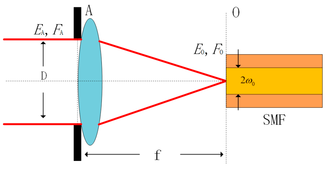
The scheme of spatial light coupling into a SMF is shown in Figure 1. The laser beam in the FSOC link generally travels a long distance, so we consider the beam entering the receiving terminal as a plane wave. E_A is the light field at the pupil plane A, while E_O is the light field on the focal plane O after the plane wave passes through the lens (usually an Airy spot). The mode-field radius of the SMF is small and only the fundamental mode transmission is allowed in the SMF, so the process of the plane wave coupling into the SMF through the focusing lens can be considered the filtering effect of the spatial filter with a radius of ω₀ placed at the focus on the optical field E_O. In line with many other researchers [22,23,24], we use the fiber mode field to be coupled Gaussian, not J/K Bessel functions, for convenience. The transfer function of the spatial filter is:

$$F_O(r,\theta )=\sqrt{\frac{2}{\pi {\omega }_0^2}}\exp (-\frac{r^2}{{\omega }_0^2})$$

(1)

where ω₀ is the mode-field radius of SMF and (r,θ) are the polar coordinates of a certain point in the focal plane O. Polar coordinates are adopted in this paper to analyze wavefront aberrations.

We calculated the influence of different wavefront aberrations on the CE in plane A for convenience, because this can avoid Fourier transform of Zernike polynomial, simplify the mathematical process and achieve fast calculation. The backpropagated mode-field of the SMF can be expressed as follows [31]:

$$F_A(r,\theta )=F^{-1}[F_O(r,\theta )]=\sqrt{\frac{2}{\pi {\omega }_a^2}}\exp (-\frac{r^2}{{\omega }_a{}^2})$$

(2)

$${\omega }_a^{}=\frac{\lambda f}{\pi {\omega }_0^{}}$$

(3)

where ω_a is the radius of backpropagated SMF mode-field radius, f is the focal length of the coupling lens, and λ is the wavelength of laser.

Here, we consider the intensity of the incident beam to be uniform and only the phase of the wavefront to change as we observe the influence of spatial frequency characteristics of aberrations on the CE. The laser wave field can be expressed as:

$$E_A(r)=E_s\exp [-j\varphi (r,\theta )]$$

(4)

where E_s is the amplitude of incident light transmission and φ(r,θ) is the phase of incident light wave field. The CE can be expressed as [23,24]:

$$\eta =\frac{{\left|{\displaystyle \int E_A{}^{*}(r)F_A(r)ds}\right|}^2}{{\displaystyle \int {\left|E_A(r)\right|}^{2}ds}{\displaystyle \int {\left|F_A(r)\right|}^{2}ds}}$$

(5)

The integral range S is the effective full aperture of the entrance pupil plane. Substituting Equations (1)–(4) into Formula (5) yields the following CE expression:

$$\begin{array}{ll}\eta & =\frac{{\left|{\displaystyle \iint E_A{}^{*}(r,\theta )F_A(r,\theta )}rdrd\theta \right|}^2}{{\displaystyle \iint {\left|E_A(r,\theta )\right|}^{2}rdrd\theta }\cdot {\displaystyle \iint {\left|F_A(r,\theta )\right|}^{2}rdrd\theta }}\\ & ={\left|{\displaystyle \iint \exp [-j\varphi (r,\theta )]\cdot \sqrt{\frac{2}{\pi {\omega }_{\alpha }{}^2}}\exp (-\frac{r^2}{{\omega }_{\alpha }{}^2})rdrd\theta }\right|}^2\\ & =\frac{2}{\pi {\omega }_{\alpha }{}^2}({\alpha }_r{}^2+{\alpha }_j{}^2)\end{array}$$

(6)

where

$${\alpha }_r={\displaystyle \iint \exp (-\frac{r^2}{{\omega }_{\alpha }{}^2})\cos [\varphi (r,\theta )]rdrd\theta }$$

(7)

$${\alpha }_j={\displaystyle \iint \exp (-\frac{r^2}{{\omega }_{\alpha }{}^2})\sin [\varphi (r,\theta )]rdrd\theta }$$

(8)

The Zernike polynomial is generally adopted to decompose the wavefront phase with distortion to a sum of weighted orthogonal polynomials, which represent various types of aberrations. Wavefront phase φ(r,θ) can be expressed as follows:

$$\varphi (r,\theta )={\alpha }_0+{\displaystyle \sum _{i=1}^{\infty }{\alpha }_i{Z}_i(r,\theta )}$$

(9)

where Z_i(r,θ) indicates the ith Zernike polynomial and a_i is the coefficient of polynomials. There are at least six different schemes available for Zernike polynomials. In order to facilitate the classification of the aberration spatial pattern, in this paper we use Noll–Zernike polynomials [32]:

$$\begin{array}{r}\begin{array}{l}{Z}_{even\begin{array}{c}\end{array}j}=\sqrt{n+1}{R}_n^m\left(r\right)\sqrt{2}\cos m\theta \\ Z_{odd\begin{array}{c}\end{array}j}=\sqrt{n+1}{R}_n^m\left(r\right)\sqrt{2}\sin m\theta \end{array}\}\begin{array}{cc}& \end{array}m\ne 0\\ Z_j=\sqrt{n+1}{R}_n^0\left(r\right) m=0\end{array}$$

(10)

where

$$R_n^m(r)={\displaystyle \sum _{s=0}^{(n-m)/2}\frac{{\left(-1\right)}^s(n-s)!}{s!\left[(n+m)/2-s\right]!\left[(n-m)/2-s\right]!}}{r}^{n-2s}$$

(11)

The relationships between n, m, and j are as follows:

$$n={[{(2j-1)}^{1/2}+0.5]}_{\mathrm{integer}}-1$$

(12)

$$m=\{\begin{array}{l}2{\left\{\left[2j+1-n(n+1)\right]/4\right\}}_{\mathrm{integer}}\mathrm{when}n\mathrm{is}\mathrm{even}\\ 2{\left\{\left[2(j+1)-n(n+1)\right]/4\right\}}_{\mathrm{integer}}-1\mathrm{when}n\mathrm{is}\mathrm{odd}\end{array}$$

(13)

Each Z_i(r,θ) can be represented by a pair (n,m) where n is the radial degree and m is the azimuthal degree. The relationship between Z_i(r,θ) and (n,m) is shown in

Table 1. Noll–Zernike Polynomial Sequence.

	m	0	1	2	3	4	5	6	7	8
n
0		Z1									circularly symmetric
1			Z2Z3
2		Z4		Z5Z6							tilt-coma
3			Z7Z8		Z9Z10						astigmatic
4		Z11		Z12Z13		Z14Z15
5			Z16Z17		Z18Z19		Z20Z21
6		Z22		Z23Z24		Z25Z26		Z27Z28
7			Z29Z30		Z31Z32		Z33Z34		Z35Z36
8		Z37		Z38Z39		Z40Z41		Z42Z43		Z44Z45

. The spatial frequency of the aberration increases as n increases. Asides from the features similar to other Zernike polynomials, the Noll–Zernike polynomial has some unique characteristics: When m = 0, only circularly symmetric aberrations exist; when m = 1, only tilt-coma items exist; and with a particular n(n ≥ 2), when m reaches its maximum, astigmatic items exist. On this basis, we analogize the effects of different single aberrations on CE.

3. Numerical Results and Analysis

3.1. Effects of Spatial Frequency Characteristics

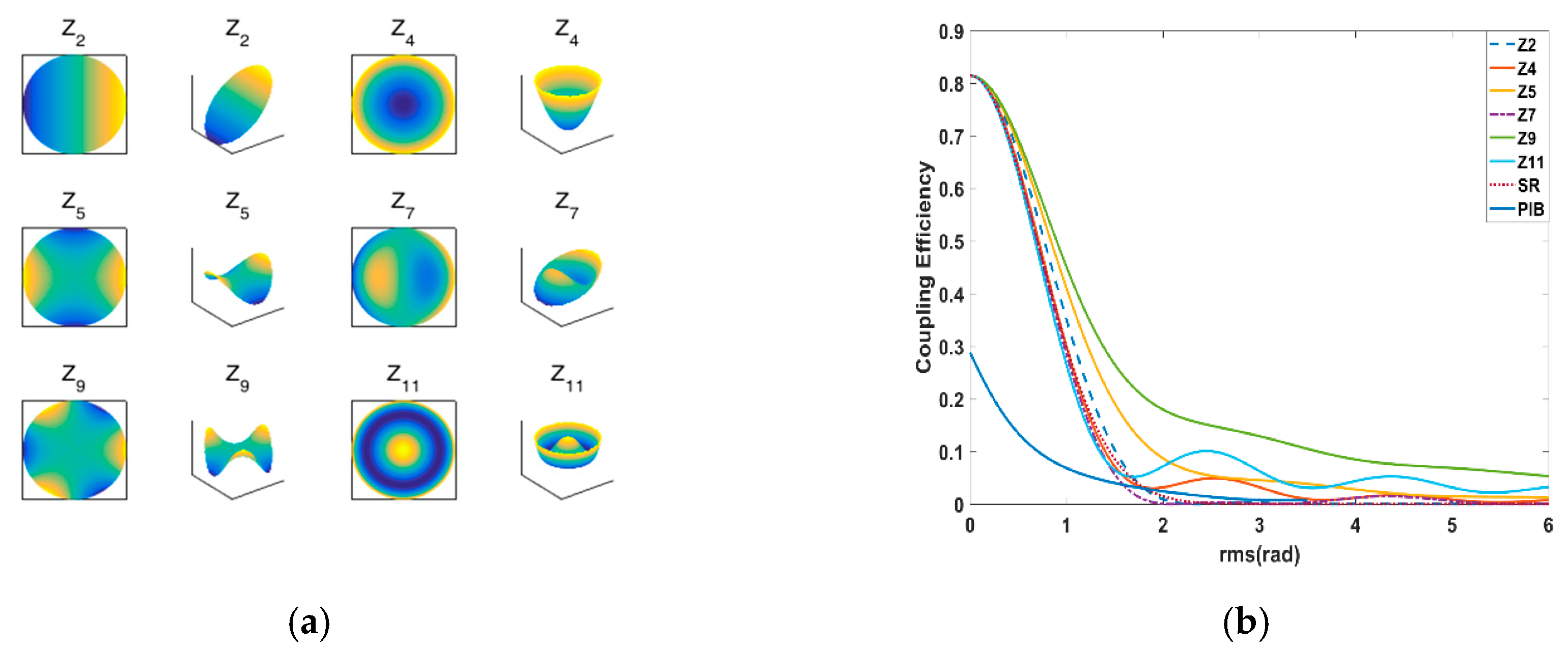
Equations (6)–(8) show that the CE of SMF depends on the matching between the incident beam wavefront and the SMF mode-field. Equation (9) is used to represent the incident beam wavefront. Figure 2a shows the pattern of first three-order Zernike aberrations and Figure 2b shows the relationship between these aberrations and the CE as analyzed by the proposed method, the SR approximation method, and the PIB method. The approximate formula for SR is [23]:

$${\mathrm{CE}}_{\mathrm{SRmethod}}\approx \exp (-{\varphi }^2)\times {\mathrm{CE}}_{\max }$$

(14)

where CE_max is the max CE without wavefront aberration, which for the SMF is 81.45% usually; and the PIB method formula is [27]:

$$\begin{array}{cc}\hfill {\mathrm{CE}}_{\mathrm{PIBmethod}}& =\pi {\left(\frac{\mathrm{D}}{2\lambda f^2}\right)}^2\times {\displaystyle {\int }_0^2\left(0.15l^4-0.275l^3-l^2+2l\right)}\times \hfill \\ & \left[{\displaystyle {\int }_{-\infty }^{\infty }\cos \left({\Phi }_r\right)\frac{1}{\sqrt{\pi \cdot 2{\varphi }_{}^2}}\exp \left(-\frac{{\Phi }_r{}^2}{2{\varphi }_{}^2}\right)d{\Phi }_r}\right]\times \frac{2{\omega }_0{J}_1\left(\pi {\omega }_{0}l\right)}{l}dl.\hfill \end{array}$$

(15)

φ is the root-mean-square (RMS) of wavefront phase, D is the beam diameter, f is the focal length, Φ is the phase structure function of incident wavefront, and l is the distance between any two points.

Based on the theory discussed above, we next analyzed the influence of aberrations of different spatial frequencies on the CE under the condition that λ = 1550 nm, w₀ = 5.2 μm, beam diameter D = 1.2 m and relative aperture D/f = 0.211.

Both SR and PIB methods can only calculate the relationship between the RMS value of the whole wavefront phase and the CE, so they do not reflect the influence of different aberration spatial frequencies on CE. By contrast, the proposed method reflects differences in different wavefront on CE even though the RMS of wavefront is the same; the differences are particularly obvious when the aberration amplitude is larger than 2 rad. The SR method has a high similarity with Z4 terms in the small aberration part. However, large errors occurred under the PIB method as it is mainly based on the calculation of geometrical optical information and generally used for the coupling calculation of few-mode and multi-mode optical fibers.

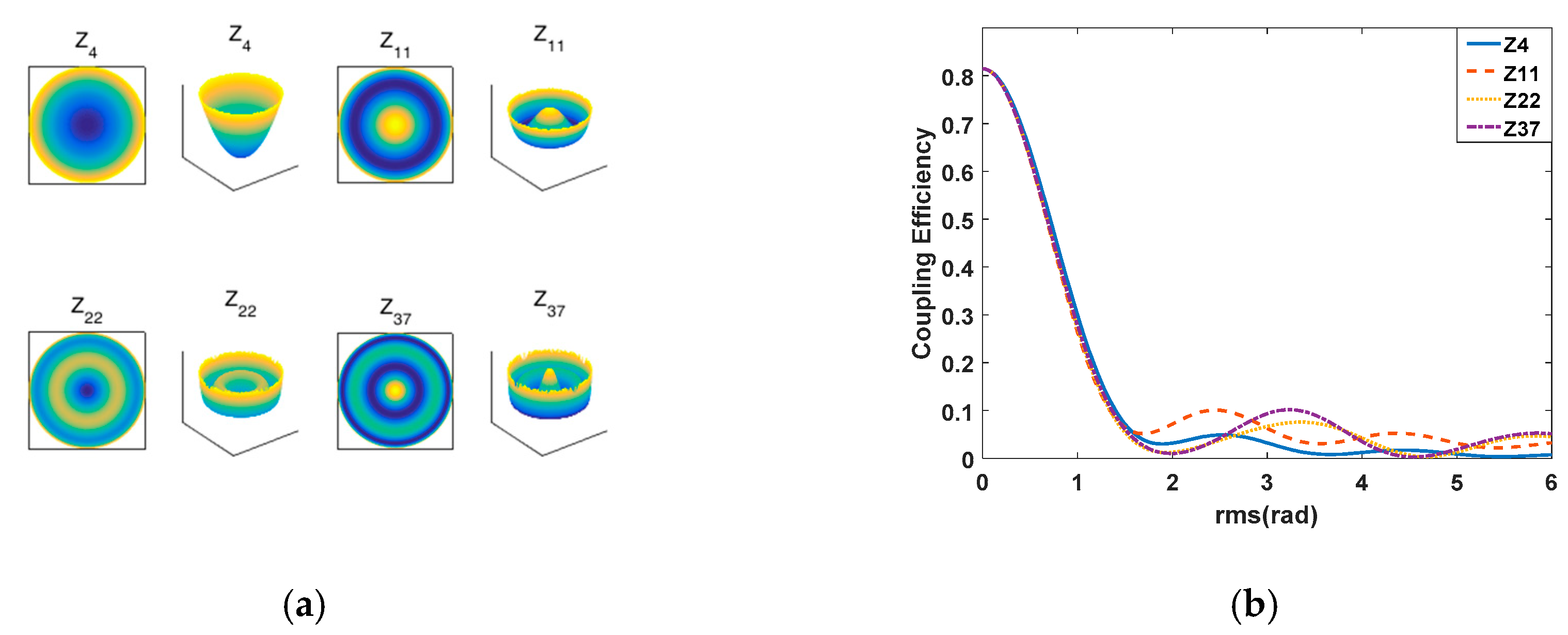
We next further classified the aberrations, beginning with the circularly symmetric aberration (m = 0) as shown in Figure 3. The overall trend of the curve for this item’s aberration on CE is consistent. Before 1.5 rad, the values are almost identical; above 1.5 rad, various oscillations emerged.

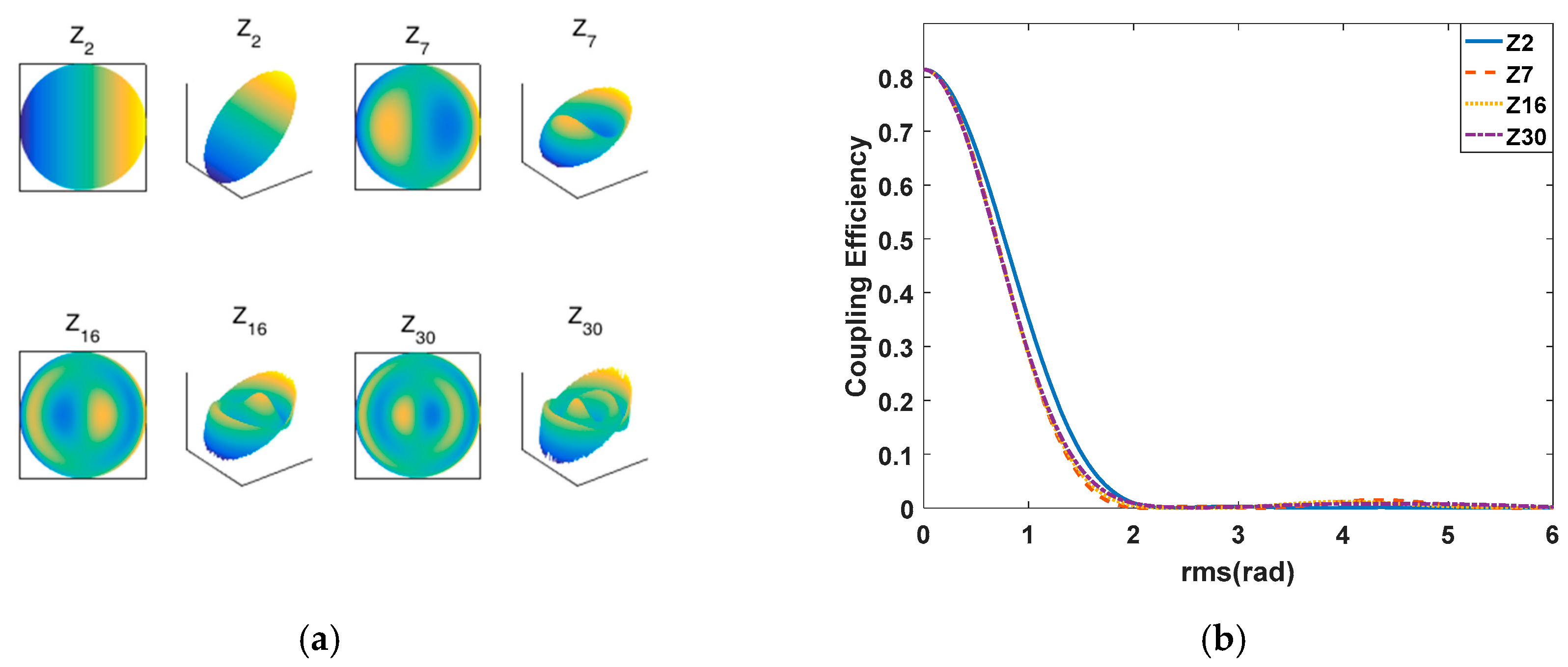
Figure 4 shows the patterns and the relationship between the tilt-coma item (m = 1) and CE. These aberrations have a similar effect on CE in that they all decay rapidly within 2 rad. When the aberration is greater than 2 rad, the CE is almost 0.

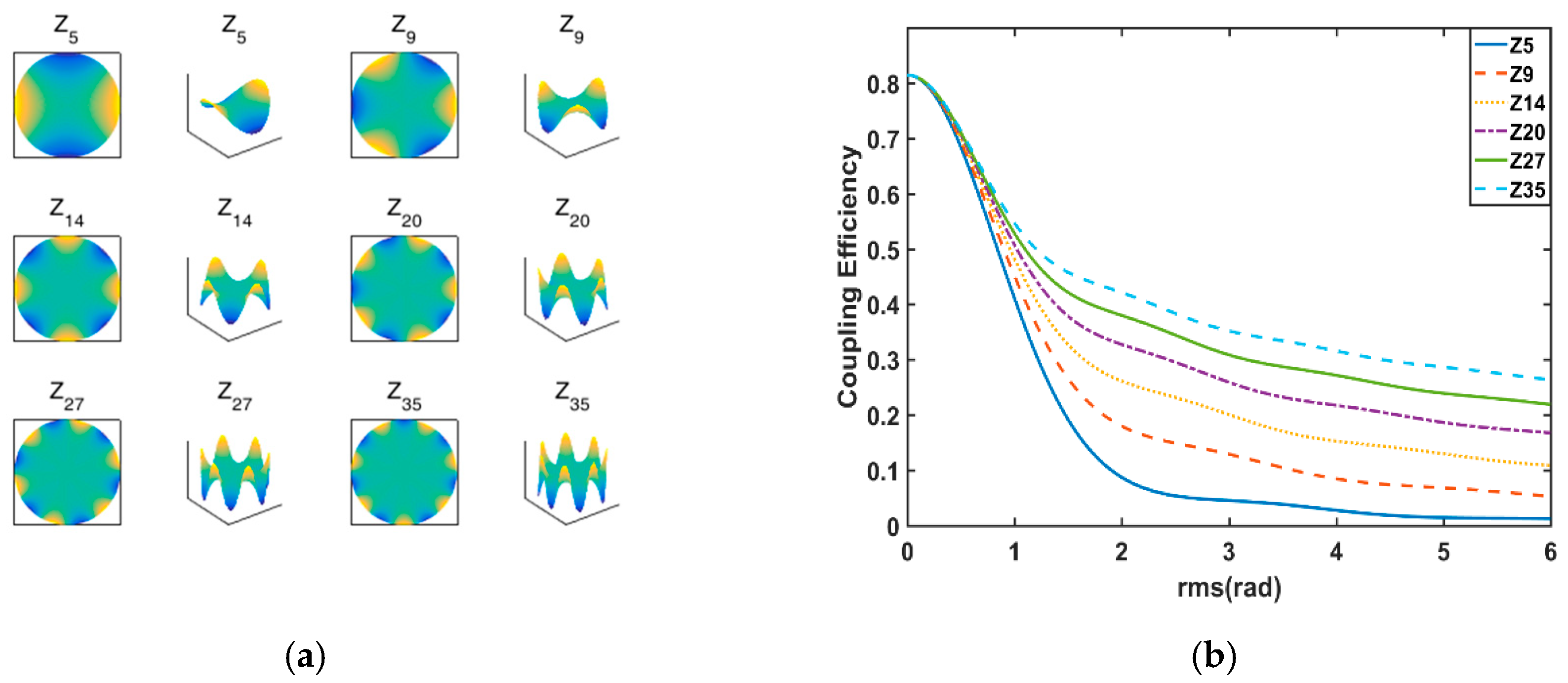
The effects of m = max, the astigmatic aberration item, on CE are shown in Figure 5b. There is rapid CE attenuation in the early stage (within 0.5 rad) and gentle attenuation with continued increase in the RMS of aberration. In addition, for this kind of aberration, when the RMS value of aberration is the same, the higher the spatial frequency of aberration, the larger the corresponding CE. The reason is, as shown in Figure 5a, for this item’s aberration, when the RMS of aberrations are the same, the higher the spatial frequency, the closer the wavefront center region of the beam is to the wavefront of the plane wave. The flatter wavefront makes the central area of the Airy spot formed on the focal plane more regular, and the matching degree with the optical fiber mode-field is higher, thus higher CE is achieved.

3.2. Influence of AO System Residuals

We used the Zernike polynomial fitting method to generate wavefront simulation data according to the statistical characteristics of atmospheric turbulence and explore the effects of AO system residual aberrations on CE. Γa is the covariance matrix of Zernike coefficient vector a for simulating the atmospheric wavefront [32,33]:

$$\Gamma a=\overline{a_i{a}_j}={\left(\frac{\mathrm{D}}{r_0}\right)}^{5/3}\times \frac{2.2698{(-1)}^{(n_i+n_j-2m_i)/2}{[(n_i+1)(n_j+1)]}^{1/2}\Gamma ((n_i+n_j-5/3)/2)}{\Gamma ((n_i-n_j+17/3)/2)\Gamma ((n_j-n_i-17/3)/2)\Gamma ((n_i+n_j+23/3)/2)}$$

(16)

We generated atmospheric turbulence simulation wavefront data with normalized atmospheric turbulence strength D/r₀ ranging from 0.5 to 15, where r₀ is the Fried parameter. We also analyzed the CE of different correction residuals of a FSOC AO system and the correction residuals margin of the AO system. The parameters in the simulation were D = 1.2 m, λ = 1550 nm, ω₀ = 5.2 μm, D/f = 0.204 and ε = 0.2 (center occlusion ratio for the Kassai Green telescope).

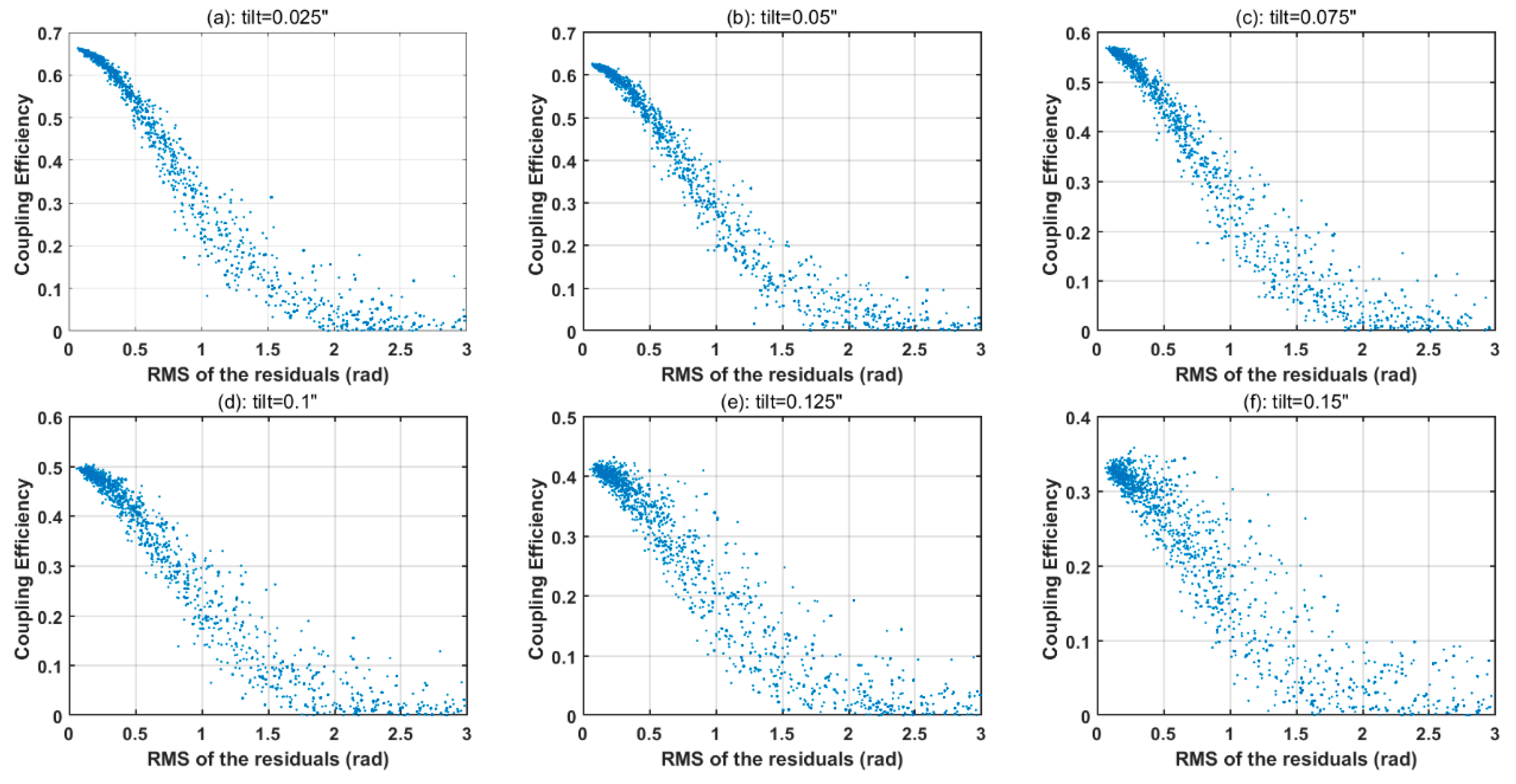
The typical AO system uses a fast steering mirror (FSM) to correct the tilt aberration and a deformable mirror (DM) to correct the aberrations expect tilt separately, so we analyzed the relationship between CE and residual aberrations (tip/tilt removed) under different tilt bias conditions. For convenience, the tilt amplitude is given here in arc-seconds while the remaining aberrations are given in the form of the overall RMS. The results are shown in Figure 6.

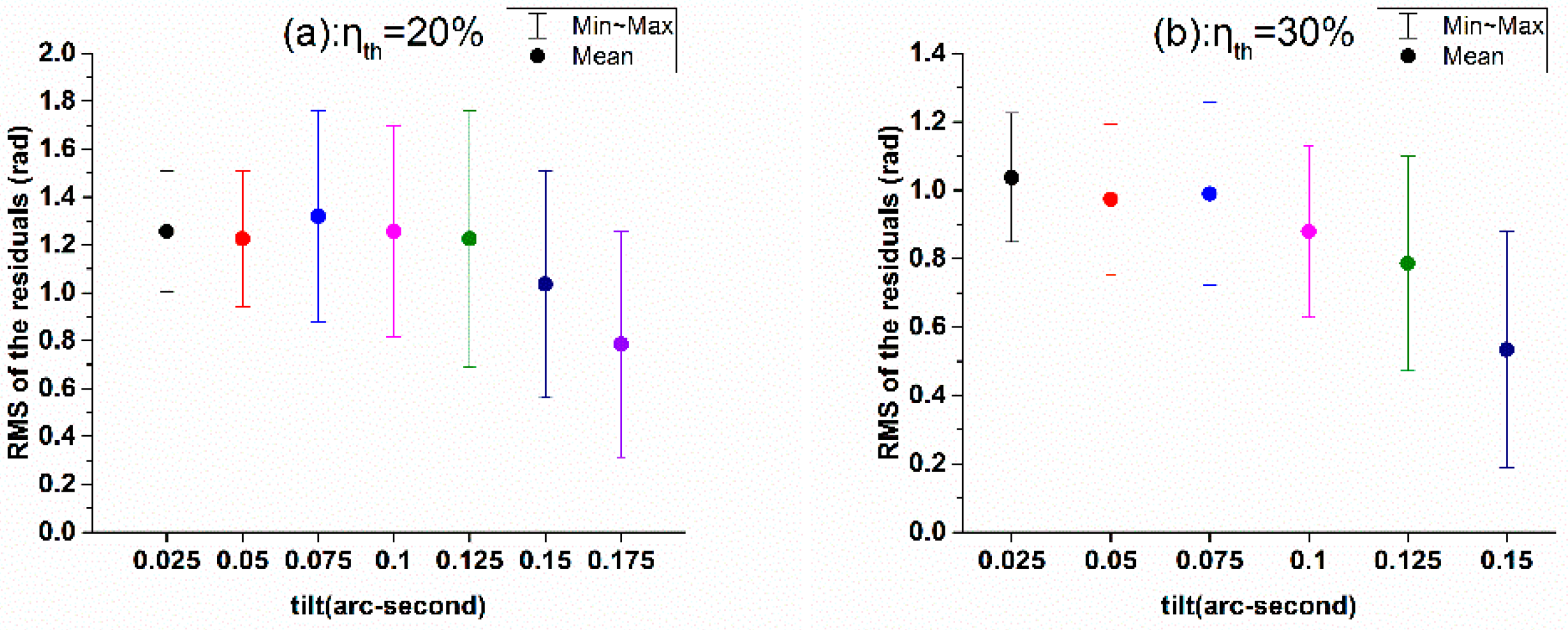
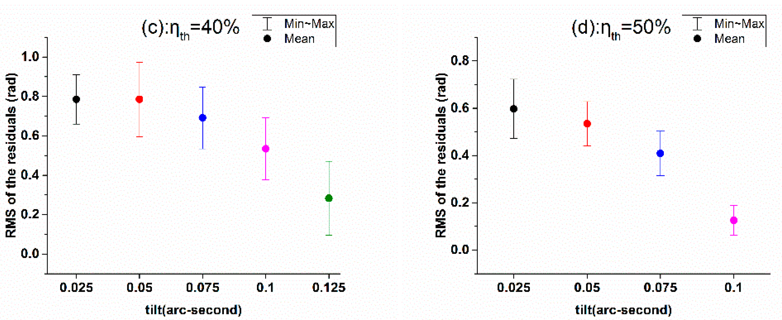
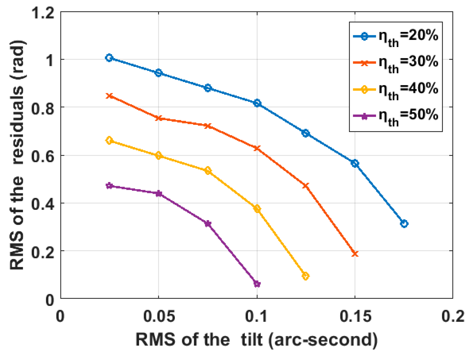
Figure 7 shows the processed results of all simulation data under different coupling thresholds (η_th), encompassing the range of aberrations that reach the CE threshold under certain tilt bias conditions. The margin of the AO system residuals differ across these conditions. As the tilt residual increases, the margin of residuals except the tilt decreases; that is, the residual of the FSM increases, which reduces the tolerance of the system for the DM correction residual.

Figure 8 shows the residual control range of the AO system under different coupling thresholds. The abscissa is the tilt magnitude, which is the FSM residual. The ordinate is the RMS of residual wavefront without tilt, i.e., the DM residual. If the coupling threshold is 30%, then the FSM and DM residuals should fall within the range enclosed by the orange curve and the coordinate axis. Our results suggest that when designing the AO system for FSOC, the correction residuals of FSM and DM should be reasonably allocated under the coupling threshold according to the system requirements.

4. Experimental Verification

4.1. Experimental Setup

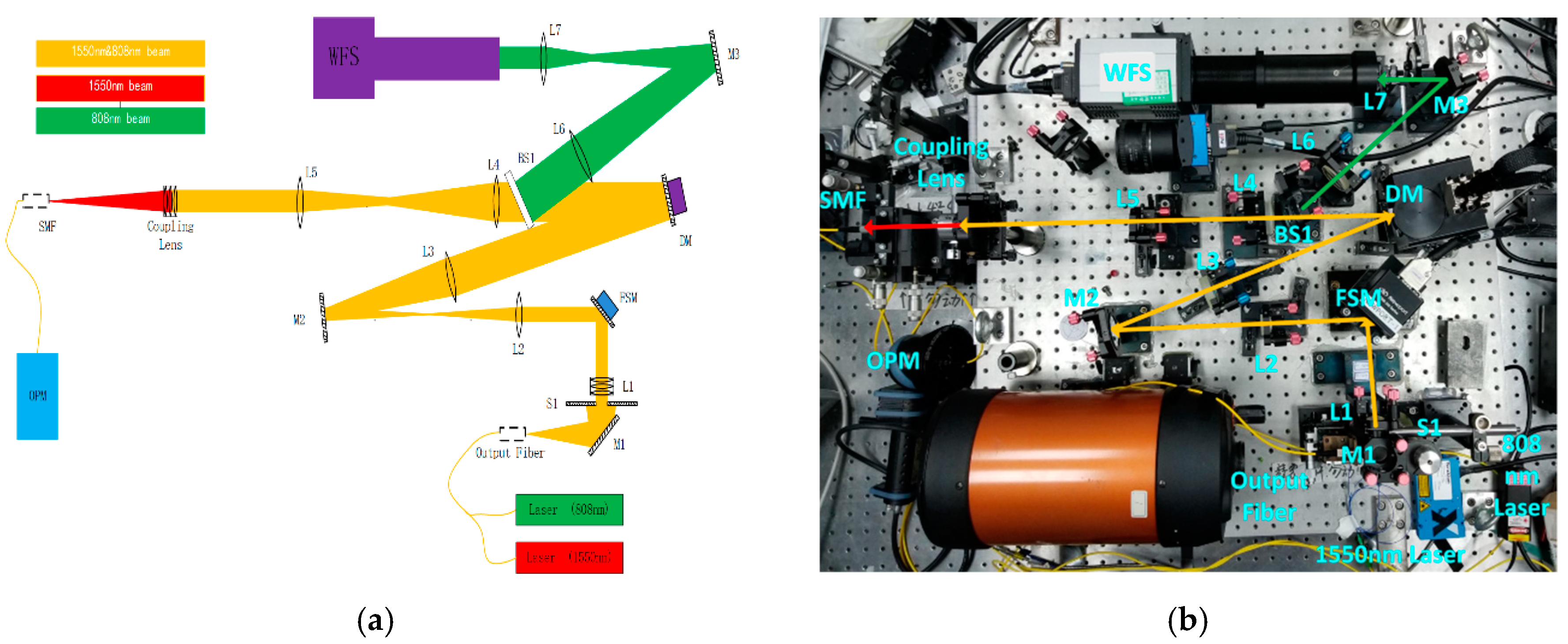
We established the experimental system shown in Figure 9 to validate our CE calculation model and theoretical analysis. Figure 9a shows a schematic diagram of the system and Figure 9b shows a photograph of the system. We established the calculation model in the case of parallel light incidence, in order to obtain ideal experimental results, we kept the optical power emitted by the light source as stable as possible throughout the experiment. We expanded the beam and used an aperture stop to intercept the center part of the beam with a relatively uniform power to weaken any variations caused by changes in the laser beam direction, which also made the power distribution of the beam more uniform. The DM is used to generate different single aberrations. In order to reduce the experimental error and improve the accuracy of the aberration fitting, we calibrated the DM fitting aberration by interferometer before the experiment. In the experiment, we use a Hartmann wavefront sensor (WFS) to measure the DM to generate aberrations in real time, and based on the measured values of WFS, estimate the wavefront aberration at the entrance of the coupling lens.

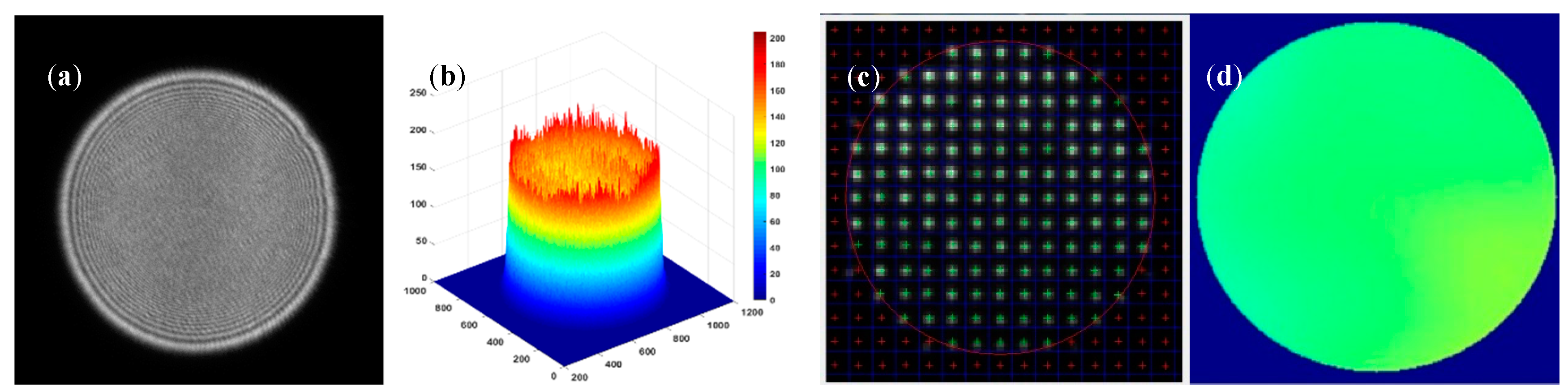
The working principle of the experimental optical system is as follows: 808 nm and 1550 nm lasers are emitted from single-mode optical fibers by a combination of optical fiber combiners. After passing through mirrors, M1 and aperture stop S1, they are expanded by the beam expander group L1 and output as the light source of the system. After being reflected by the FSM, the collimated beam is further expanded by L2 and L3; after being reflected by DM, it enters the beam splitter BS1. Next, 80% of the 808 nm light is reflected by BS1 and enters the WFS after being compressed by L6 L7. The remaining 20% of the 808 nm light and all the 1550 nm light pass through BS1 and are compressed by L4 L5 into a beam of 10 mm diameter before reaching the coupling lens. The 1550 nm light is coupled into the SMF after being focused by the coupling lens, while the 808 nm light is filtered out. We used image sensor and WFS to measure the intensity and wavefront phase of the initial 808 nm beam after being expanded and corrected, and used it as the basis for evaluating the quality of the 1550 nm coupled beam. The results are shown in Figure 10, the standard deviation of the power fluctuation of the beam is 15.78 gray value, and the RMS value of the wavefront phase is 0.0239λ (λ = 808 nm).

The model and parameters of the equipment used in the experiment are as follows: The 1550 nm laser is PS-NLL210816 from TeraXion, the 808 nm laser is 808-030-SM01 from SFOLT, the FSM is a FSM-300 from Newport, the DM is a DM145-25 from ALPAO with 145 actuators in its 30 mm aperture. The Hartmann WFS has a lens array consisting of a 2.3 mm diameter 15 * 15 microlens array. The coupling lens has an effective aperture of 20 mm and a focal length of 50 mm. The SMF placed at the receiving end is a SMF-28e which has a mode-field diameter of 10.4 um at 1550 nm.

4.2. Experimental Results and Analysis

The DM was controlled to generate single aberrations of different amplitudes as we measured the influence curve of each single aberration on the CE. We used the normalized CE to express our experimental results to reflect the similarity between the measured data and theoretical calculated value, which is aimed to reduce the influence of errors in components and optical path. The theoretical calculated value in the figures below takes into account the Fresnel reflection and transmission loss, which was calculated as the energy loss by 4%, and the theoretical calculated curve of the SR approximation method is also added for comparison.

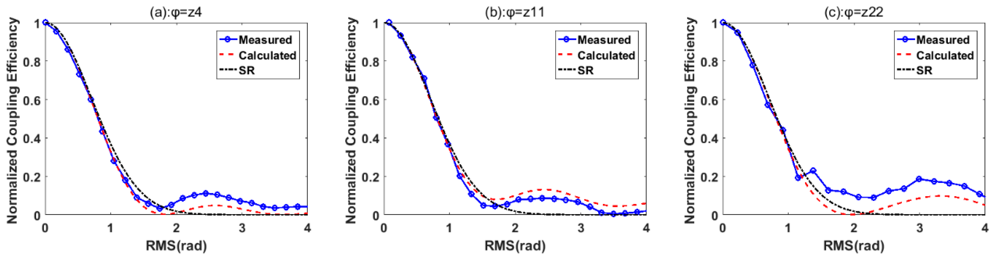
As shown in Figure 11, the measured CE curves of the three aberrations Z4, Z11, and Z22 are almost the same as the theoretical values in the small aberration range. Although the values in the large aberration range show some deviation, the maximum error is less than 0.12, and the measured data are consistent with the curve trends of the theoretical values.

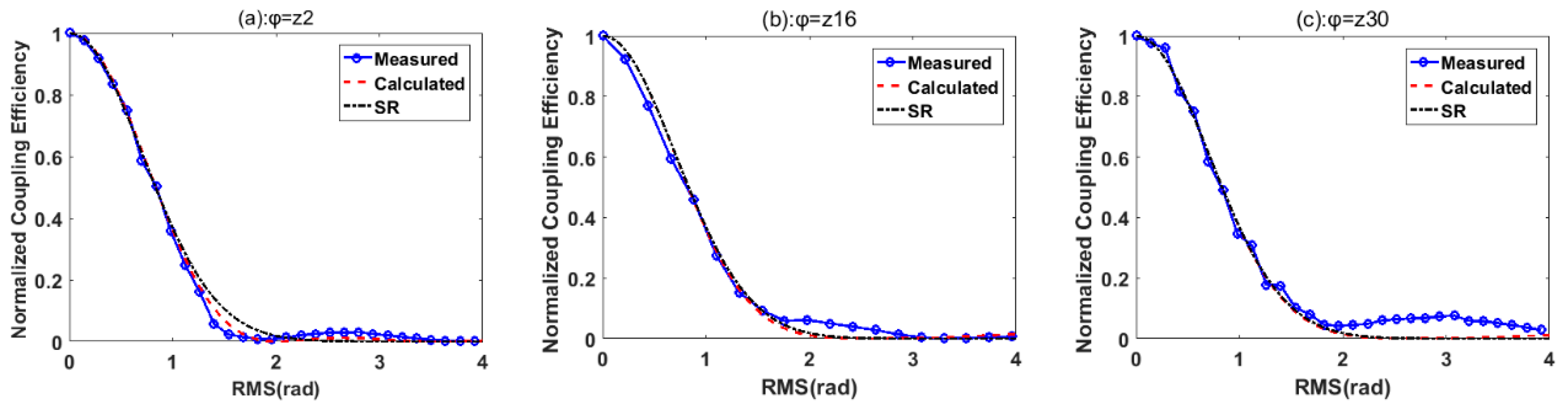
The relation between tilt-coma items and CE is shown in Figure 12. Figure 12a shows the influence of tilt (Z2) on CE, where the measured CE has a local maximum value (between 2–3 rad) formed by the secondary diffraction ring of the Airy disk. As shown in Figure 12b,c, the measured CE curves of Z16 and Z30 deviated from theoretical calculations, which can be possibly attributed to the crosstalk of the same terms and the error of aberration generation. The maximum error between measured and calculated values is no more than 0.076.

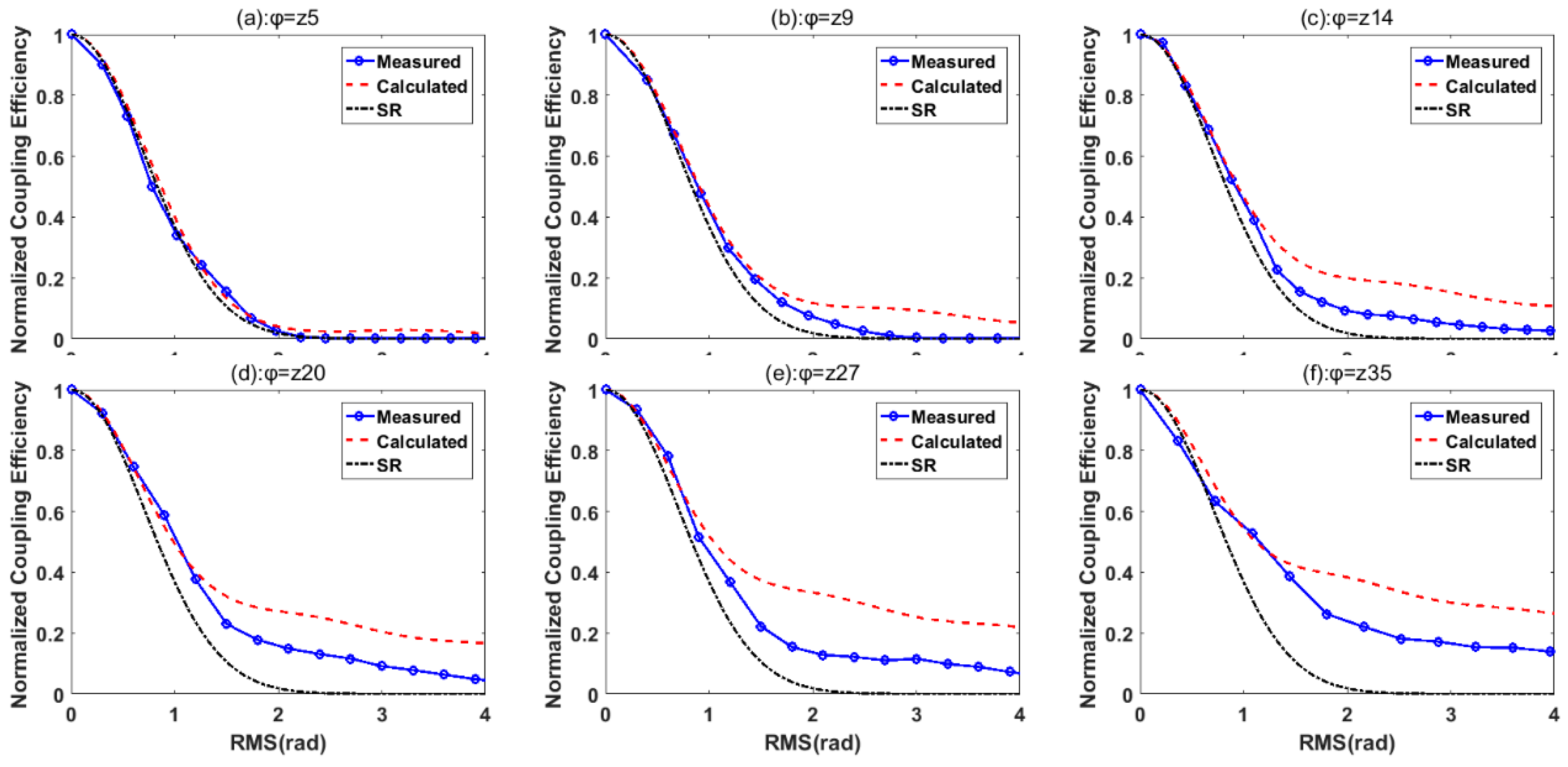
Figure 13 shows the influence curve of astigmatic aberrations on CE. Although the experimentally measured CE is lower than the theoretically calculated value with the maximum error less than 0.2, the trend of measured data curve is the same as the theoretical curve. More importantly, as the spatial frequency of the aberration increases, the CE in the large aberration regime also increases, which is fully consistent with the theoretical analysis results.

Under small aberration (RMS < 1.5 rad) conditions, the experimental data is almost completely consistent with the theoretical curve. However, when RMS > 1.5 rad, the influence of DM fitting ability and Hartmann WFS detection accuracy introduced other aberrations in addition to the desired single aberration; this caused deviation between the measured and theoretical CE values. The experimental results validate the proposed CE calculation method as well as our analysis of the influence of spatial frequency and other factors on CE.

5. Conclusions

We analyzed the effects of aberrations on the CE of spatial light coupled into SMF based on single-aberration spatial characteristics in this study. We found that the effects of the same type of aberrations on the CE are similar, but the CE values are different as the spatial frequency changes. We also assessed the influence of the AO system residual on CE and determined the corrected residual margins of FSM and DM for a FSOC system under different coupling threshold conditions. Finally, we validated our analysis results with a series of experiments.

Based on the analysis results of the influence of different aberrations on CE in this paper, researchers can focus on controlling the aberrations which have great influence on CE in the design and alignment of optical systems, so as to minimize the impact of the optical system on CE. For ALTD applications such as FSOC and GSL, researchers can make better residual margin allocation for AO systems in these applications based on the results of this study. Through selectivity, devices such as FSM, DM and WFS can better meet the system requirements, so as to improve the correction effect of AO system, and ultimately achieve the improvement of CE. In addition, the results presented in this paper also have reference significance for the application of wavefront sensing technology based on single aberration mode detection, such as holographic wavefront sensor designs.

We plan to conduct further research, using WFS to directly detect the aberration generation of the 1550 nm coupled beam and make the DM operate in closed loop mode, so as to strengthen the validation of the research results of this study. What’s more, we are interested in studying how to apply Extended Nijboer–Zernike polynomials to our model in the follow-up work, so as to establish a new method which can simultaneously analyze the impact of beam intensity and phase changes on coupling efficiency. In addition, considering that we use the Gaussian function approximation to represent the fundamental mode field in this paper, which may cause some errors in the calculation results, it is also worth studying how to use Bessel function to discuss the content of this paper.

References

- Ding, J.C.; Li, M.; Tang, M.H.; Li, Y.; Song, Y.J. BER performance of MSK in ground-to-satellite uplink optical communication under the influence of atmospheric turbulence and detector noise. Opt. Lett. 2013, 38, 3488–3491. [Google Scholar] [CrossRef] [PubMed]
- Hemmati, H. Interplanetary laser communications and precision ranging. Laser Photon. Rev. 2011, 5, 697–710. [Google Scholar] [CrossRef]
- Hemmati, H.; Biswas, A.; Djordjevic, I.B. Deep-space optical communications: Future perspectives and applications. Proc. IEEE 2011, 99, 2020–2039. [Google Scholar] [CrossRef]
- Takenaka, H.; Toyoshima, M.; Takayama, Y. Experimental verification of fiber-coupling efficiency for satellite-to-ground atmospheric laser downlinks. Opt. Express 2012, 20, 15301–15308. [Google Scholar] [CrossRef] [PubMed]
- Fletcher, A.S.; Hamilton, S.A.; Moores, J.D. Undersea laser communication with narrow beams. IEEE Commun. Mag. 2015, 53, 49–55. [Google Scholar] [CrossRef]
- Yang, J.X.; Zhang, H.; Zhang, X.G.; Li, H.; Xi, L.X. Transmission characteristics of adaptive compensation for joint atmospheric turbulence effects on the OAM-based wireless communication system. Appl. Sci. 2019, 9, 901. [Google Scholar] [CrossRef]
- Qu, Z.; Djordjevic, I.B. Orbital Angular momentum multiplexed free-space optical communication systems based on coded modulation. Appl. Sci. 2018, 8, 2179. [Google Scholar] [CrossRef]
- Abadi, M.M.; Ghassemlooy, Z.; Bhatnagar, M.R.; Zvanovec, S.; Khalighi, M.A.; Lavery, M.P.J. Differential signalling in free-space optical communication systems. Appl. Sci. 2018, 8, 872. [Google Scholar] [CrossRef]
- Chen, Z.Y.; Yan, L.S.; Pan, Y.; Jiang, L.; Yi, A.L.; Pan, W.; Luo, B. Use of polarization freedom beyond polarizationdivision multiplexing to support high-speed and spectral-efficient data transmission. Light Sci. Appl. 2017, 6, e16207. [Google Scholar] [CrossRef]
- Hill, C. Coherent focused lidars for doppler sensing of aerosols and wind. Remote Sens. 2018, 10, 466. [Google Scholar] [CrossRef]
- Ke, X.Z.; Lei, S.C. Spatial light coupled into a single-mode fiber by a Maksutov-Cassegrain antenna through atmospheric turbulence. Appl. Opt. 2016, 55, 3897–3902. [Google Scholar] [CrossRef]
- Ozdur, I.; Toliver, P.; Woodward, T.K. Photonic-lantern-based coherent LIDAR system. Opt. Express 2015, 23, 5312–5316. [Google Scholar] [CrossRef]
- Li, G.; Li, J.Q. A pulse shaping based optical transmission system of 128QAM for DWDM with N x 904 Gbps. Appl. Sci. 2019, 9, 988. [Google Scholar] [CrossRef]
- Lundberg, L.; Karlsson, M.; Lorences-Riesgo, A.; Mazur, M.; Torres-Company, V.; Schroder, J.; Andrekson, P.A. Frequency comb-based WDM transmission systems enabling joint signal processing. Appl. Sci. 2018, 8, 718. [Google Scholar] [CrossRef]
- Chen, J.H.; Zheng, B.C.; Shao, G.H.; Ge, S.J.; Xu, F.; Lu, Y.Q. An all-optical modulator based on a stereo graphene-microfiber structure. Light Sci. Appl. 2015, 4, e360. [Google Scholar] [CrossRef]
- Xiong, W.; Hsu, C.W.; Bromberg, Y.; Antonio-Lopez, J.E.; Correa, R.A.; Cao, H. Complete polarization control in multimode fibers with polarization and mode coupling. Light Sci. Appl. 2018, 7, 54. [Google Scholar] [CrossRef]
- Liu, J.; Li, S.M.; Zhu, L.; Wang, D.; Chen, S.; Klitis, C.; Du, C.; Mo, Q.; Sorel, M.; Yu, S.Y.; et al. Direct fiber vector eigenmode multiplexing transmission seeded by integrated optical vortex emitters. Light Sci. Appl. 2018, 7, 17148. [Google Scholar] [CrossRef]
- Xie, Z.W.; Lei, T.; Li, F.; Qiu, H.D.; Zhang, Z.C.; Wang, H.; Min, C.J.; Du, L.P.; Li, Z.H.; Yuan, X.C. Ultra-broadband on-chip twisted light emitter for optical communications. Light Sci. Appl. 2018, 7, 18001. [Google Scholar] [CrossRef]
- Dianov, E.M. Bismuth-doped optical fibers: A challenging active medium for near-IR lasers and optical amplifiers. Light Sci. Appl. 2012, 1, e12. [Google Scholar] [CrossRef]
- Hadzievski, L.; Maluckov, A.; Rubenchik, A.M.; Turitsyn, S. Stable optical vortices in nonlinear multicore fibers. Light Sci. Appl. 2015, 4, e314. [Google Scholar] [CrossRef]
- Willner, A.E. Vector-mode multiplexing brings an additional approach for capacity growth in optical fibers. Light Sci. Appl. 2018, 7, 18002. [Google Scholar] [CrossRef]
- Wagner, R.E.; Tomlinson, W.J. Coupling efficiency of optics in single-mode fiber componentS. Appl. Opt. 1982, 21, 2671–2688. [Google Scholar] [CrossRef]
- Ruilier, C. A study of degraded light coupling into single-mode fibers. In Astronomical Interferometry, Pts 1 and 2; Reasenberg, R.D., Ed.; International Society for Optics and Photonics: Bellingham, WA, USA, 1998; Volume 3350, pp. 319–329. [Google Scholar]
- Ma, J.; Zhao, F.; Tan, L.; Yu, S.; Han, Q. Plane wave coupling into single-mode fiber in the presence of random angular jitter. Appl. Opt. 2009, 48, 5184–5189. [Google Scholar] [CrossRef]
- Ma, J.; Zhao, F.; Tan, L.Y.; Yu, S.Y.; Yang, Y.Q. Degradation of single-mode fiber coupling efficiency due to localized wavefront aberrations in free-space laser communications. Opt. Eng. 2010, 49, 6. [Google Scholar] [CrossRef]
- Yin, X.H.; Wang, R.; Wang, S.X.; Wang, Y.K.; Jin, C.B.; Cao, Z.L.; Xuan, L. Evaluation of the communication quality of free-space laser communication based on the power-in-the-bucket method. Appl. Opt. 2018, 57, 573–581. [Google Scholar] [CrossRef]
- Wang, R.; Wang, Y.K.; Jin, C.B.; Yin, X.H.; Wang, S.X.; Yang, C.L.; Cao, Z.L.; Mu, Q.Q.; Gao, S.J.; Xuan, L. Demonstration of horizontal free-space laser communication with the effect of the bandwidth of adaptive optics system. Opt. Commun. 2019, 431, 167–173. [Google Scholar] [CrossRef]
- Zhu, X.L.; Wang, K.L.; Wang, F.; Zhao, C.L.; Cai, Y.J. Coupling Efficiency of a Partially Coherent Radially Polarized Vortex Beam into a Single-Mode Fiber. Appl. Sci. 2018, 8, 1313. [Google Scholar] [CrossRef]
- Chen, M.; Liu, C.; Rui, D.; Xian, H. Performance verification of adaptive optics for satellite-to-ground coherent optical communications at large zenith angle. Opt. Express 2018, 26, 4230–4242. [Google Scholar] [CrossRef]
- Chen, M.; Liu, C.; Xian, H. Experimental demonstration of single-mode fiber coupling over relatively strong turbulence with adaptive optics. Appl. Opt. 2015, 54, 8722–8726. [Google Scholar] [CrossRef]
- Wallner, O.; Winzer, P.J.; Leeb, W.R. Alignment tolerances for plane-wave to single-mode fiber coupling and their mitigation by use of pigtailed collimators. Appl. Opt. 2002, 41, 637–643. [Google Scholar] [CrossRef]
- Noll, R.J. Zernike polynomials and atmospheric-turbulence. J. Opt. Soc. Am. 1976, 66, 207–211. [Google Scholar] [CrossRef]
- Roddier, N. Atmospheric wave-front simulation using zernike polynomials. Opt. Eng. 1990, 29, 1174–1180. [Google Scholar] [CrossRef]
© 2019 by the authors. Licensee MDPI, Basel, Switzerland. This article is an open access article distributed under the terms and conditions of the Creative Commons Attribution (CC BY) license (http://creativecommons.org/licenses/by/4.0/).