Active Fault-Tolerant Control of a Quadcopter against Time-Varying Actuator Faults and Saturations Using Sliding Mode Backstepping Approach

Featured Application

This work addresses issues related to fault-tolerant control of quadcopter UAVs.

Abstract

Fault-tolerant control is becoming an interesting topic because of its reliability and safety. This paper reports an active fault-tolerant control method for a quadcopter unmanned aerial vehicle (UAV) to handle actuator faults, disturbances, and input constraints. A robust fault diagnosis based on the $H_{\infty }$ scheme was designed to estimate the magnitude of a time-varying fault in the presence of disturbances with unknown upper bounds. Once the fault estimation was complete, a fault-tolerant control scheme was proposed for the attitude system, using adaptive sliding mode backstepping control to accommodate the actuator faults, despite actuator saturation limitation and disturbances. The Lyapunov theory was applied to prove the robustness and stability of the closed-loop system under faulty operation. Simulation results show the effectiveness of the fault diagnosis scheme and proposed controller for handling actuator faults.

1. Introduction

The quadcopter unmanned aerial vehicles (UAVs) have drawn attention for their potential use in a wide range of technologies and applications due to their reliability, agility, mechanical simplicity, and ability to operate in narrow and dangerous spaces both in outdoor and indoor environments. This adaptability and reliability promote its universality over other UAV systems. Therefore, quadcopter UAVs have been investigated and applied in different technologies, including precision landing [1,2], formation flight [3,4], fault-tolerant control [5,6] and trajectory tracking [7,8].

Currently, the vertical and horizontal movements of a quadcopter are controlled by a pilot with a remote-control system, whereas angular movement is automatically controlled by an onboard flight controller. The attitude controller is more crucial for maintaining the quadcopter at an appropriate coordinate, because it not only allows the quadcopter to achieve the desired attitude, but also avoids crashing when the pilot operates the desired vertical and horizontal movements [9]. During operation, one critical issue with the attitude controller is the uncertainties of the model and the disturbances that the quadcopter encounters. Previous studies have proposed various control schemes, such as backstepping control [10,11], fuzzy control [12,13], sliding mode control [14,15], and neural network technique [16,17], to handle this problem. When faults occur, solving the control problem to guarantee the stability of the quadcopter becomes a greater challenge [18], because this control problem could lead to a flight failure. Therefore, fault-tolerant control (FTC) is an important factor that should be examined intensively while designing the attitude controller.

Recently, the study of FTC has enabled researchers to reinforce the safety and reliability of systems. Generally, the types of faults examined in FTC systems are process, actuator, and sensor faults. The actuator is a crucial element in obtaining a specific rotation for translation, because it can connect to the control signals. Therefore, the actuator faults were investigated in this work. There are two methods to handle this kind of faults: Passive FTC (PFTC) and active FTC (AFTC). Previous studies have focused on PFTC approaches to accommodate the actuator faults using a robust controller that does not depend on robust fault detection and the fault estimation scheme. Different methods have been proposed based on adaptive control, feedback linearization, and $H_{\infty }$ adaptive control [19,20,21]. These methods are good for fault compensation, but they are not sufficiently robust for disturbances and uncertainties if the system matrices are not accurate. To overcome this problem, several nonlinear techniques have been proposed based on sliding mode control, adaptive sliding mode control, neural network control, fuzzy control, and backstepping control [22,23,24,25,26,27,28,29,30,31]. These studies present robust controllers for fault accommodation. The above-mentioned PFTC methods can address faults in fault-free and faulty operations. However, in PFTC schemes, the magnitude of faults is designed in a given boundary.

To handle the large magnitude of faults, AFTC using a fault detection and identification unit, has been proposed [32]. Various approaches based on sliding mode control for the quadcopter have been investigated. For instance, several authors have proposed a sliding mode control based on active and passive FTC [33]. In this work, the PFTC mode in fault-free operation was switched over to AFTC when a fault was detected. The experimental results on Qball-X4 showed that the AFTC method can compensate better than PFTC during tracking. When faults occur in an actuator, both methods can successfully drive the quadrotor. This work also compared the merits and demerits of each approach. An on-line FTC method is also proposed based on the control allocation technique and sliding mode control [34]. When faults occur in an actuator, the control allocation scheme uses the effectiveness level of the actuator to redistribute the control signals to the remaining fault-free actuators. In another famous study using a sliding mode fault-tolerant controller, a fault detection unit was generated from a linear observer [18]. When a fault was detected, a reconfiguration technique was used by scarifying the yaw control. The simulation results showed that the reconfiguration scheme could conduct a good tracking operation in the presence of partial loss in nominal thrust. The advantage of this method is that it was able to reject disturbances and uncertainties in fault-free operation. Another study proposed the sliding mode observer and sliding mode control for the AFTC scheme [35]. In this work, the fault estimation from the sliding mode observer was injected into the sliding mode controller for reconfiguration. The results show the effectiveness of this method in the presence of disturbances and uncertainties. Recently, there was a study on tracking control for a quadrotor using sliding mode and backstepping control [15]. The results showed that the proposed method could handle the chattering phenomenon and uncertainties, but this approach was complicated because it used the fuzzy method, which is a trial and error method. Moreover, that work did not focus on an actuator fault in a quadcopter model, which is what motivates us to conduct this study. An active FTC method for actuator fault control in the presence of disturbances and uncertainties is proposed in this paper. This method offers robust control for time-varying actuator faults and saturation, which was limited in previous studies. The main contributions of this study, over the previous ones, can be summarized as follows:

• The fault diagnosis based on $H_{\infty }$ technique [36] is introduced to estimate the time-varying faults.
• The AFTC based adaptive sliding mode backstepping [15] was improved here to ensure that the tracking performance converges to zero in spite of time-varying, actuator faults and disturbances.
• A modified AFTC is proposed to handle the input saturation.
• Stability analysis in presented to verify the robustness of the proposed controller.

The remaining article is organized as follows. Section 2 introduces the quadcopter dynamics. The active fault-tolerant control based on adaptive sliding mode backstepping control and $H_{\infty }$ technique for attitude system is discussed in Section 3. Section 4 presents the simulation results. The conclusions and recommendations for future work are provided in Section 5.

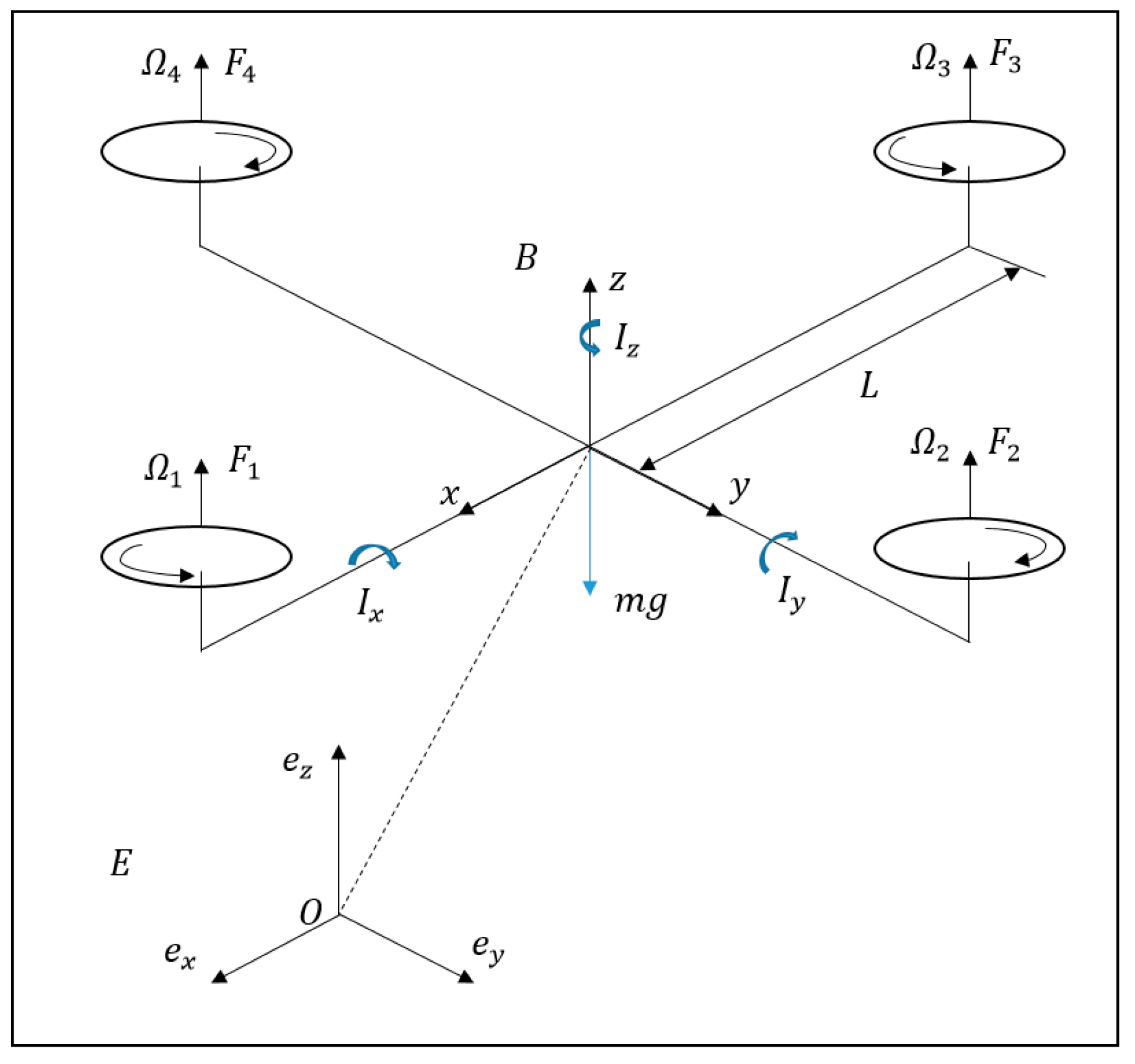
2. Quadcopter Modeling

A quadcopter is subjected to torques and forces (Figure 1). Quadcopter dynamics are examined in an inertial frame, B and an earth frame, E. The quadcopter model consisted of two counterclockwise and two clockwise rotating motors. The arm length is denoted by $L$. The dynamics of the quadcopter can be described as follows [37,38,39,40,41,42,43,44]:

$$\{\begin{array}{l}\ddot{\varphi }=\left(U_{\varphi }+(I_y-I_z)\dot{\theta }\dot{\psi }-{\overline{J}}_m\dot{\theta }\Omega -K_1\dot{\varphi }\right)/I_x\\ \ddot{\theta }=\left(U_{\theta }+(I_z-I_x)\dot{\varphi }\dot{\psi }-{\overline{J}}_m\dot{\varphi }\Omega -K_2\dot{\theta }\right)/I_y\\ \ddot{\psi }=\left(U_{\psi }+(I_x-I_y)\dot{\varphi }\dot{\theta }-K_3\dot{\psi }\right)/I_z\\ \ddot{x}=\left\{U_T(\cos \varphi \sin \theta \cos \psi +\sin \varphi \sin \psi )-K_4\dot{x}\right\}/m\\ \ddot{y}=\left\{U_T(\cos \varphi \sin \theta \sin \psi -\sin \varphi \sin \psi )-K_5\dot{y}\right\}/m\\ \ddot{z}=-g+\left\{U_T(\cos \varphi \cos \theta )-K_6\dot{z}\right\}/m\end{array}$$

(1)

where $I_x,I_y,I_z$ are the moments of inertia along the $x,y,z$ directions, respectively; $K_1,K_2,K_3,K_4,K_5$ and $K_6$ are drag terms; ${\overline{J}}_m$ is the moment of inertia of an individual motor, and with ${\omega }_i$ being the rotational speed produced by the $i\mathrm{th}$ motor; $m$ is the total mass; $\varphi ,\theta ,$ and $\psi$ are the Euler angles including roll, pitch, and yaw, respectively; $x,y,$ and $z$ denote the position of the quadcopter; and the four control inputs can be presented as:

$$\{\begin{array}{l}{U}_T=F_1+F_2+F_3+F_4\\ U_{\varphi }=(F_4-F_2)L\\ U_{\theta }=(F_3-F_1)L\\ U_{\psi }={\tau }_1-{\tau }_2+{\tau }_3-{\tau }_4\end{array}$$

(2)

where ${\tau }_i=d{\omega }_i^2$ and $F_i=b{\omega }_i^2$ represent the torques and thrust forces, respectively, induced by the $i\mathrm{th}$ motor; $b$ and $d$ are positive constants, and $U_T$ is the total thrust; $U_{\varphi },U_{\theta }$ and $U_{\psi }$ are the torques in the roll, pitch, and yaw directions.

The relationship between thrust force and control inputs (Equation (2)) can be rewritten as:

$$\left[\begin{array}{l}{U}_T\\ U_{\varphi }\\ U_{\theta }\\ U_{\psi }\end{array}\right]=\left[\begin{array}{cccc}1& 1& 1& 1\\ 0& -L& 0& L\\ -L& 0& L& 0\\ d/b& -d/b& d/b& -d/b\end{array}\right]\left[\begin{array}{l}{F}_1\\ F_2\\ F_3\\ F_4\end{array}\right]$$

(3)

The bound of control inputs can be calculated as:

$$\{\begin{array}{l}0\le U_T\le 4b{\omega }_{\max }^2\\ -bL{\omega }_{\max }^2\le U_{\varphi }\le bL{\omega }_{\max }^2\\ -bL{\omega }_{\max }^2\le U_{\theta }\le bL{\omega }_{\max }^2\\ -d{\omega }_{\max }^2\le U_{\psi }\le d{\omega }_{\max }^2\end{array}$$

(4)

where ${\omega }_{\max }$ is the maximum velocity of each actuator.

3. Active Fault-Tolerant Control System Design

The active fault-tolerant control scheme is presented in this section. The control structure is shown in Figure 2. First, a fault diagnosis unit is proposed to estimate the magnitude of actuator faults. Then, a modified adaptive sliding mode backstepping (MASMBC) control is designed to tolerate actuator faults by combining the fault estimation and adaptive sliding mode back stepping control (ASMBC).

3.1. Fault Diagnosis Scheme

In this section, the designing of a fault estimation scheme through an adaptive observer in the presence of actuator faults and external disturbances is presented. This information is used for controller design, which is presented in Section 3.2.

By defining $x^T=\left[\begin{array}{cccccccc}\varphi & \theta & \psi & z& \dot{\varphi }& \dot{\theta }& \dot{\psi }& \dot{z}\end{array}\right]$ as the state vector, $u^T=\left[\begin{array}{cccc}{F}_1& F_2& F_3& F_4\end{array}\right]=\left[\begin{array}{cccc}{u}_1& u_2& u_3& u_4\end{array}\right]$ as the control force vector, and $y=\left[\begin{array}{cccccccc}\varphi & \theta & \psi & z& \dot{\varphi }& \dot{\theta }& \dot{\psi }& \dot{z}\end{array}\right]$ as the output vector, and using linearization technique for z-direction and attitude system at hovering point [37], Equation (1) can be rewritten in a state-space form as:

$$\{\begin{array}{l}\dot{x}(t)=Ax(t)+Bu(t)+H+E_{d}d(t)\\ y=Cx(t)\end{array}$$

(5)

where $E_d$ is the disturbance matrix, $d(t)$ is the disturbance vector, $E_d=I_{8\times 8},$ $A=\left[\begin{array}{cc}{0}_{4\times 4}& I_{4\times 4}\\ 0_{4\times 4}& 0_{4\times 4}\end{array}\right],$$B=\left[\begin{array}{cccc}0& 0& 0& 0\\ 0& 0& 0& 0\\ 0& 0& 0& 0\\ 0& 0& 0& 0\\ 0& -L/I_x& 0& L/I_x\\ -L/I_y& 0& L/I_y& 0\\ d/(b{I}_z)& -d/(b{I}_z)& d/(b{I}_z)& -d/(b{I}_z)\\ 1/m& 1/m& 1/m& 1/m\end{array}\right],$$C=I_{8\times 8}$, and $H={\left[\begin{array}{cccccccc}0& 0& 0& 0& 0& 0& 0& -g\end{array}\right]}^T$.

When a fault occurs in the actuator, Equation (5) becomes [37]:

$$\{\begin{array}{l}\dot{x}(t)=Ax(t)+Bu(t)-BU(t)\Delta (t)+H+E_{d}d(t)\\ y=Cx(t)\end{array}$$

(6)

where $U(t)=\left[\begin{array}{cccc}{u}_1(t)& 0& 0& 0\\ 0& u_2(t)& 0& 0\\ 0& 0& u_3(t)& 0\\ 0& 0& 0& u_4(t)\end{array}\right]$; $\Delta (t)=\left[\begin{array}{l}{\vartheta }_1(t)\\ {\vartheta }_2(t)\\ {\vartheta }_3(t)\\ {\vartheta }_4(t)\end{array}\right]$ is the loss of control effectiveness matrix, $0\le {\vartheta }_i(t)\le 1;i=1,\dots ,4$; ${\vartheta }_i(t)=0$ and ${\vartheta }_i(t)=1$ means that the ith actuator is completely healthy or fully damaged, respectively.

The state space model (Equation (6)) can be rewritten as:

$$\{\begin{array}{l}\dot{x}(t)=Ax(t)+Bu(t)+Bf(t)+H+E_{d}d(t)\\ y=Cx(t)\end{array}$$

(7)

where $f(t)=-U(t)\Delta (t)$.

Before designing the adaptive observer, the following assumptions and lemmas are proposed.

Assumption 1.

$\dot{f}(t)$ is norm-bounded, i.e., $\Vert \dot{f}(t)\Vert \le f_1$, with $f_1>0$.

Lemma 1.

For a given matrix$P=P^T\ge 0$and scalar$\rho >0$, the following inequality must be satisfied:

$$2x^{T}y\le {\rho }^{-1}{x}^{T}Px+\rho y^T{P}^{-1}y$$

(8)

If all the above-mentioned assumptions and lemmas hold, then the adaptive observer can be constructed as:

$$\{\begin{array}{l}\dot{\widehat{x}}(t)=A\widehat{x}(t)+Bu(t)+B\widehat{f}(t)+H+L(y(t)-\widehat{y}(t))\\ \widehat{y}=C\widehat{x}(t)\end{array}$$

(9)

Theorem 1.

For a given observer gain,$L$, constant$\epsilon >0$, if there exist the matrices$P=P^T>0,G=G^T>0,\Lambda ={\Lambda }^T>0,R_1$and$R_2$such that:

$$\left[\begin{array}{ccc}{M}_{11}& M_{12}& M_{13}\\ \ast & M_{22}& M_{23}\\ \ast & \ast & M_{33}\end{array}\right]<0$$

(10)

$$B^{T}P=R_{1}C$$

(11)

where $M_{11}={(A-LC)}^{T}P+P(A-LC)+C^{T}C$, $M_{12}={(A-LC)}^T{C}^T{R}_2^T$, $M_{13}=P{E}_d$, $M_{22}={\rho }^{-1}G-2R_{2}CB$, $M_{23}=-R_{2}C{E}_d$, $M_{33}=-{\epsilon }^2{I}_p$, $\eta ={\rho }^{-1}{f}_1^2{\lambda }_{\max }({\Lambda }^{-1}{G}^{-1}{\Lambda }^{-1})$, and $I_p$ is the unitary matrix with appropriate dimension, then, the fault estimation law can be presented as:

$$\dot{\widehat{f}}(t)=\rho \Lambda R_1{e}_y(t)+\rho \Lambda R_2{\dot{e}}_y(t)$$

(12)

Stability

Let

$$\begin{array}{l}{e}_x(t)=x(t)-\widehat{x}(t)\\ e_f(t)=f(t)-\widehat{f}(t)\end{array}$$

(13)

then the error dynamics can be obtained from Equations (7) and (9) as:

$${\dot{e}}_x(t)=\left(A-LC\right)e_x(t)+B{e}_f(t)+E_{d}d(t)$$

(14)

Let us consider the following Lyapunov candidate:

$$V(t)=e_x^T(t)P{e}_x(t)+{\rho }^{-1}{e}_f^T(t){\Lambda }^{-1}{e}_f(t)$$

(15)

Its time derivative $\dot{V}(t)$ is:

$$\begin{array}{lll}\dot{V}(t)& =& {\dot{e}}_x^T(t)P{e}_x(t)+e_x^T(t)P{\dot{e}}_x(t)\\ & & +2{\rho }^{-1}{e}_f^T(t){\Lambda }^{-1}{\dot{e}}_f(t)\\ & =& e_x^T(t)\left[{(A-LC)}^{T}P+P(A-LC)\right]e_x(t)\\ & & +2e_x^T(t)PB{e}_f(t)+2e_x^T(t)P{E}_{d}d(t)\\ & & +2{\rho }^{-1}{e}_f^T(t){\Lambda }^{-1}(\dot{f}(t)-\dot{\widehat{f}}(t))\end{array}$$

(16)

Substituting Equations (11), (12), and (14) into Equation (16) we obtain:

$$\begin{array}{ll}\dot{V}(t)=& e_x^T(t)\left[{(A-LC)}^{T}P+P(A-LC)\right]e_x(t)\\ & +2e_x^{T}P{E}_{d}d(t)+2{\rho }^{-1}{e}_f^T(t){\Lambda }^{-1}\dot{f}(t)\\ & -2e_f^T{R}_{2}C(A-LC)e_x-2e_f^T{R}_{2}CB{e}_f\\ & -2e_f^T{R}_{2}C{E}_{d}d(t)\end{array}$$

(17)

From Lemma 1, Assumption 1, and Theorem 1, we obtain:

$$\begin{array}{l}2{\rho }^{-1}{e}_f^T(t){\Lambda }^{-1}\dot{f}(t)\\ \le {\rho }^{-1}(e_f^T(t)G{e}_f^T(t)+{\dot{f}}^T(t){\Lambda }^{-1}{G}^{-1}{\Lambda }^{-1}\dot{f}(t))\\ \le {\rho }^{-1}(e_f^T(t)G{e}_f^T(t)+f_1^2{\lambda }_{\max }({\Lambda }^{-1}{G}^{-1}{\Lambda }^{-1}))\end{array}$$

(18)

where ${\lambda }_{\max }$ is the maximum eigenvalue of the associated matrix.

The $H_{\infty }$ tracking index function is chosen to ensure that the adaptive observer is robust against the external disturbance as:

$$J={\displaystyle \underset{0}{\overset{\infty }{\int }}\left[e_y^T(t)e_y(t)-{\epsilon }^2{d}^T(t)d(t)\right]\mathrm{d}t}$$

(19)

With the initial conditions $(V(0)=0,V(\infty )>0)$, we obtain:

$$\begin{array}{ll}J& ={\displaystyle \underset{0}{\overset{\infty }{\int }}\left[e_y^T(t)e_y(t)-{\epsilon }^2{d}^T(t)d(t)+\dot{V}(t)\right]\mathrm{d}t}+V(0)-V(\infty )\\ & \le {\displaystyle \underset{0}{\overset{\infty }{\int }}\left[e_x^T(t)C^{T}C{e}_x(t)-{\epsilon }^2{d}^T(t)d(t)+\dot{V}(t)\right]\mathrm{d}t}\end{array}$$

(20)

From Equation (19), the integral term can be described as:

$$\begin{array}{lll}N& =& e_x^T\left({(A-LC)}^{T}P+P(A-LC)+C^{T}C\right)e_x\\ & & +2e_x^{T}P{E}_{d}d(t)+{\rho }^{-1}{e}_f^T(t)G{e}_f(t)\\ & & +{\rho }^{-1}{f}_1^2{\lambda }_{\max }({\Lambda }^{-1}{G}^{-1}{\Lambda }^{-1})-2e_f^T{R}_{2}C(A-LC)e_x\\ & & -2e_f^T{R}_{2}CB{e}_f-2e_f^T{R}_{2}C{E}_{d}d(t)-{\epsilon }^2{d}^T(t)d(t)\\ & =& {\left[\begin{array}{l}{e}_x(t)\\ e_f(t)\\ d(t)\end{array}\right]}^T\left[\begin{array}{ccc}{M}_{11}& M_{12}& M_{13}\\ \ast & M_{22}& M_{23}\\ \ast & \ast & M_{33}\end{array}\right]\left[\begin{array}{l}{e}_x(t)\\ e_f(t)\\ d(t)\end{array}\right]\end{array}$$

(21)

where

$$\begin{array}{l}{M}_{11}={(A-LC)}^{T}P+P(A-LC)+C^{T}C\\ M_{12}={(A-LC)}^T{C}^T{R}_2^T\\ M_{13}=P{E}_d\\ M_{22}={\rho }^{-1}G-2R_{2}CB\\ M_{23}=-R_{2}C{E}_d\\ M_{33}=-{\epsilon }^2{I}_p\\ \eta ={\rho }^{-1}{f}_1^2{\lambda }_{\max }({\Lambda }^{-1}{G}^{-1}{\Lambda }^{-1})\end{array}$$

If the following inequality holds:

$$\left[\begin{array}{ccc}{M}_{11}& M_{12}& M_{13}\\ \ast & M_{22}& M_{23}\\ \ast & \ast & M_{33}\end{array}\right]<0$$

(22)

when we have $N<n{I}_n$ and thus can obtain $J<\eta$.

Remark 1.

To solve Equations (10) and (11) simultaneously, the linear matrix inequalities (LMI) technique was applied to relax these conditions. Equation (11) was modified according to previous study [5].

$$\left[\begin{array}{cc}{\eta }_{1}I& B^{T}P-R_{1}C\\ {(B^{T}P-R_{1}C)}^T& {\eta }_{1}I\end{array}\right]>0$$

(23)

3.2. Adaptive Sliding Mode Fault-Tolerant Controller Design

In this part, the ASMBC is proposed in Section 3.2.1 to handle fault disturbances and time-varying actuator faults in attitude systems through adaptive law and fault estimation as seen in Section 3.1. Then, a modified ASMBC is designed to address the input constraints, which is presented in Section 3.2.2.

3.2.1. Adaptive Sliding Mode Controller Design without Input Saturations

Under faulty operation, Equation (1) can be rewritten as:

$$\{\begin{array}{l}\ddot{\varphi }=\left({\overline{U}}_{\varphi }+(I_y-I_z)\dot{\theta }\dot{\psi }-{\overline{J}}_m\dot{\theta }\Omega -K_1\dot{\varphi }\right)/I_x\\ \ddot{\theta }=\left({\overline{U}}_{\theta }+(I_z-I_x)\dot{\varphi }\dot{\psi }-{\overline{J}}_m\dot{\varphi }\Omega -K_2\dot{\theta }\right)/I_y\\ \ddot{\psi }=\left({\overline{U}}_{\psi }+(I_x-I_y)\dot{\varphi }\dot{\theta }-K_3\dot{\psi }\right)/I_z\\ \ddot{x}=\left\{{\overline{U}}_T(\cos \varphi \sin \theta \cos \psi +\sin \varphi \sin \psi )-K_4\dot{x}\right\}/m\\ \ddot{y}=\left\{{\overline{U}}_T(\cos \varphi \sin \theta \sin \psi -\sin \varphi \sin \psi )-K_5\dot{y}\right\}/m\\ \ddot{z}=-g+\left\{{\overline{U}}_T(\cos \varphi \cos \theta )-K_6\dot{z}\right\}/m\end{array}$$

(24)

where ${\overline{U}}_{\varphi },{\overline{U}}_{\theta },{\overline{U}}_{\psi },{\overline{U}}_T$ are the control inputs for faulty operation denoted by:

$$\{\begin{array}{l}{\overline{U}}_T={\overline{F}}_1+{\overline{F}}_2+{\overline{F}}_3+{\overline{F}}_4\\ {\overline{U}}_{\varphi }=L\left({\overline{F}}_4-{\overline{F}}_2\right)\\ {\overline{U}}_{\theta }=L\left({\overline{F}}_3-{\overline{F}}_1\right)\\ {\overline{U}}_{\psi }=d\left({\overline{F}}_1-{\overline{F}}_2+{\overline{F}}_3-{\overline{F}}_4\right)/b\end{array}$$

(25)

Let $\Delta {\vartheta }_i={\vartheta }_i-{\widehat{\vartheta }}_i$ be the estimation error, the actuator fault model can be written as:

$${\overline{F}}_i=(1-{\vartheta }_i)F_i=(1-{\widehat{\vartheta }}_i)F_i-\Delta {\vartheta }_i{F}_i$$

(26)

From Equations (24)–(26), we obtain:

$$\{\begin{array}{l}\ddot{\varphi }=\left(U_{\varphi }+(I_y-I_z)\dot{\theta }\dot{\psi }-{\overline{J}}_m\dot{\theta }\Omega -K_1\dot{\varphi }\right)/I_x+{\xi }_1+{\zeta }_1\\ \ddot{\theta }=\left(U_{\theta }+(I_z-I_x)\dot{\varphi }\dot{\psi }-{\overline{J}}_m\dot{\varphi }\Omega -K_2\dot{\theta }\right)/I_y+{\xi }_2+{\zeta }_2\\ \ddot{\psi }=\left(U_{\psi }+(I_x-I_y)\dot{\varphi }\dot{\theta }-K_3\dot{\psi }\right)/I_z+{\xi }_3+{\zeta }_3\\ \ddot{x}=\frac{\left\{U_T(\cos \varphi \sin \theta \cos \psi +\sin \varphi \sin \psi )-K_4\dot{x}\right\}}{m}+{\xi }_4+{\zeta }_4\\ \ddot{y}=\frac{\left\{U_T(\cos \varphi \sin \theta \sin \psi -\sin \varphi \sin \psi )-K_5\dot{y}\right\}}{m}+{\xi }_5+{\zeta }_5\\ \ddot{z}=-g+\frac{\left\{U_T(\cos \varphi \cos \theta )-K_6\dot{z}\right\}}{m}+{\xi }_6+{\zeta }_6\end{array}$$

(27)

where

$$\{\begin{array}{l}{\xi }_1=-L\left({\widehat{\vartheta }}_4{F}_4-{\widehat{\vartheta }}_2{F}_2\right)/I_x\\ {\xi }_2=-L\left({\widehat{\vartheta }}_3{F}_3-{\widehat{\vartheta }}_1{F}_1\right)/I_y\\ {\xi }_3=-d\left({\widehat{\vartheta }}_1{F}_1-{\widehat{\vartheta }}_2{F}_2+{\widehat{\vartheta }}_3{F}_3-{\widehat{\vartheta }}_4{F}_4\right)/b{I}_z\\ {\xi }_4=-\frac{(\cos \varphi \sin \theta \cos \psi +\sin \varphi \sin \psi )}{m}\left({\widehat{\vartheta }}_1{F}_1+{\widehat{\vartheta }}_2{F}_2+{\widehat{\vartheta }}_3{F}_3+{\widehat{\vartheta }}_4{F}_4\right)\\ {\xi }_5=-\frac{(\cos \varphi \sin \theta \sin \psi -\sin \varphi \sin \psi )}{m}\left({\widehat{\vartheta }}_1{F}_1+{\widehat{\vartheta }}_2{F}_2+{\widehat{\vartheta }}_3{F}_3+{\widehat{\vartheta }}_4{F}_4\right)\\ {\xi }_6=-\frac{\cos \varphi \cos \theta }{m}\left({\widehat{\vartheta }}_1{F}_1+{\widehat{\vartheta }}_2{F}_2+{\widehat{\vartheta }}_3{F}_3+{\widehat{\vartheta }}_4{F}_4\right)\end{array}$$

(28)

and the uncertainties from estimation errors:

$$\{\begin{array}{l}{\zeta }_1=-L\left(\Delta {\vartheta }_4{F}_4-\Delta {\vartheta }_2{F}_2\right)/I_x\\ {\zeta }_2=-L\left(\Delta {\vartheta }_3{F}_3-\Delta {\vartheta }_1{F}_1\right)/I_y\\ {\zeta }_3=-d\left(\Delta {\vartheta }_1{F}_1-\Delta {\vartheta }_2{F}_2+\Delta {\vartheta }_3{F}_3-\Delta {\vartheta }_4{F}_4\right)/b{I}_z\\ {\zeta }_4=-\frac{(\cos \varphi \sin \theta \cos \psi +\sin \varphi \sin \psi )}{m}\left(\Delta {\vartheta }_1{F}_1+\Delta {\vartheta }_4{F}_2+\Delta {\vartheta }_3{F}_3+\Delta {\vartheta }_4{F}_4\right)\\ {\zeta }_5=-\frac{(\cos \varphi \sin \theta \sin \psi -\sin \varphi \sin \psi )}{m}\left(\Delta {\vartheta }_1{F}_1+\Delta {\vartheta }_4{F}_2+\Delta {\vartheta }_3{F}_3+\Delta {\vartheta }_4{F}_4\right)\\ {\zeta }_6=-\frac{\cos \varphi \cos \theta }{m}\left(\Delta {\vartheta }_1{F}_1+\Delta {\vartheta }_4{F}_2+\Delta {\vartheta }_3{F}_3+\Delta {\vartheta }_4{F}_4\right)\end{array}$$

(29)

By defining the state vector as $\overline{x}={\left[\begin{array}{cccccc}\varphi & \dot{\varphi }& \theta & \dot{\theta }& \psi & \dot{\psi }\end{array}\right]}^T={\left[\begin{array}{cccccc}{\overline{x}}_1& {\overline{x}}_2& {\overline{x}}_3& {\overline{x}}_4& {\overline{x}}_5& {\overline{x}}_6\end{array}\right]}^T$ and the control inputs vector as $U=\left[\begin{array}{ccc}{U}_{\varphi }& U_{\theta }& U_{\psi }\end{array}\right]=\left[\begin{array}{ccc}{v}_1& v_2& v_3\end{array}\right]$, the rotational movement equations of the quadcopter become:

$$\{\begin{array}{l}{\dot{\overline{x}}}_{2i-1}={\overline{x}}_{2i}\\ {\dot{\overline{x}}}_{2i}=f_i(\overline{x},t)+g_i{v}_i(t)+{\xi }_i(\overline{x},t)+{\zeta }_i\end{array}$$

(30)

Let us define the desired attitude as ${\overline{x}}_i^d$. The control goal is to find a control law, $u_i$, such that ${\overline{x}}_{2i-1}(t)\to {\overline{x}}_i^d$ as $t\to \infty$, with $i=1,2,3$. If we define the control error as:

$$e_i={\overline{x}}_{2i-1}-{\overline{x}}_i^d$$

(31)

Then the first sliding surface can be described as:

$$s_{1i}=e_i+k_i{\displaystyle \int e_i}dt$$

(32)

where $k_i$ is the positive constant.

Let us now choose the Lyapunov function:

$$V_{1i}=\frac{1}{2}{s}_{1i}^2$$

(33)

The time derivative is given by:

$${\dot{V}}_{1i}=s_{1i}{\dot{s}}_{1i}=s_{1i}({\dot{\overline{x}}}_{2i-1}-{\dot{\overline{x}}}_i^d+k_i{e}_i)$$

(34)

The virtual control input can be defined as:

$${\alpha }_i={\dot{\overline{x}}}_i^d-k_i{e}_i-A_i{s}_{1i}$$

(35)

Substituting the virtual control value of ${\overline{x}}_{2i}$, Equation (34) becomes:

$${\dot{V}}_{1i}=-A_i{e}_i^2<0$$

(36)

then, $e_i=0$ is globally asymptotically stable.

The second sliding surface has a form as:

$$\begin{array}{ll}{s}_{2i}& ={\dot{\overline{x}}}_{2i-1}-{\alpha }_i\\ & ={\dot{\overline{x}}}_{2i-1}+k_i{e}_i+A_i{s}_{1i}-{\dot{\overline{x}}}_i^d\\ & ={\dot{e}}_i+k_i{e}_i+A_i{s}_{1i}\\ & ={\dot{s}}_{1i}+A_i{s}_{1i}\end{array}$$

(37)

From Equations (30), (31), and (37), ${\dot{s}}_{2i}$ can be written as:

$$\begin{array}{ll}{\dot{s}}_{2i}& ={\dot{\overline{x}}}_{2i}+k_i{\dot{e}}_i+A_i{\dot{s}}_{1i}-{\ddot{\overline{x}}}_i^d\\ & =f_i(\overline{x})+g_i{v}_i(t)+{\xi }_i(\overline{x},t)+{\zeta }_i\\ & +k_i{\dot{e}}_i+A_i{\dot{s}}_{1i}-{\ddot{\overline{x}}}_i^d\end{array}$$

(38)

With the sliding surface in Equations (31) and (37), the fault-tolerant control law can be expressed as:

$$v_i=\frac{1}{g_i}\left(\begin{array}{l}-f_i(x)-{\xi }_i(\overline{x},t)+{\ddot{\overline{x}}}_i^d-k_i{\dot{e}}_i\\ -A_i{\dot{s}}_{1i}-s_{1i}-{\widehat{\Gamma }}_i\mathrm{sign}(s_{2i})\end{array}\right)$$

(39)

and updated by [44]:

$${\dot{\widehat{\Gamma }}}_i={\beta }_i\left|s_{2i}\right|$$

(40)

where ${\beta }_i$ is a positive constant, and $\mathrm{sign}(.)$ denotes the sign function.

By considering the Lyapunov candidate as:

$$V_{2i}=\frac{1}{2}\frac{{\tilde{\Gamma }}_i^2}{{\beta }_i}+\frac{1}{2}(s_{1i}^2+s_{2i}^2)$$

(41)

where ${\tilde{\Gamma }}_i={\Gamma }_i-{\widehat{\Gamma }}_i$, ${\widehat{\Gamma }}_i$ is the estimate of ${\Gamma }_i$.

Its derivative is:

$$\begin{array}{ll}{\dot{V}}_{2i}& =\frac{{\tilde{\Gamma }}_i{\dot{\widehat{\Gamma }}}_i}{{\beta }_i}+s_{1i}{\dot{s}}_{1i}+s_{2i}{\dot{s}}_{2i}\\ & =-({\Gamma }_i-{\widehat{\Gamma }}_i)\left|s_{2i}\right|+s_{1i}(s_{2i}-A_i{s}_{1i})+s_{2i}{\dot{s}}_{2i}\\ & =-A_i{s}_{1i}^2-{\Gamma }_i\left|s_{2i}\right|+{\zeta }_i{s}_{2i}\\ & \le -A_i{s}_{1i}^2-({\Gamma }_i-{\zeta }_i)\left|s_{2i}\right|\end{array}$$

(42)

Assumption 2.

There exits an unknown parameter,${\Gamma }_i>0$, such that the uncertainties are assumed to be bounded$\left|{\zeta }_i\right|\le {\Gamma }_i$.

From Assumption 2, it is clear that ${\dot{V}}_{2i}\le 0$. Therefore, the adaptive sliding mode backstepping control law in Equation (39) will asymptotically stabilize the system.

Remark 2.

To avoid the chattering phenomenon, a saturation function is introduced to replace the$sign$function as:

$$\mathrm{sat}(s_{2i})=\{\begin{array}{ll}{s}_{2i}& \mathrm{if}\left|s_{2i}\right|\le 1\\ \mathrm{sign}(s_{2i})& \mathrm{if}\left|s_{2i}\right|>1\end{array},i=1,2,3$$

(43)

3.2.2. Adaptive Sliding Mode Controller Design with Input Saturations

In real applications, the controller presented in Equation (39) might not be implementable because of the saturation limit. Let us denote $v_{\max }>0,v_{\min }>0$ as the maximum and minimum control inputs. Then, the rotation movement in Equation (30) can be rewritten in presence of actuator saturation as:

$$\{\begin{array}{l}{\dot{\overline{x}}}_{2i-1}={\overline{x}}_{2i}\\ {\dot{\overline{x}}}_{2i}=f_i(\overline{x})+g_i\mathrm{sat}(v_i(t))+{\xi }_i(\overline{x},t)+{\zeta }_i\end{array}$$

(44)

Theorem 2.

Let us consider the faulty operation with actuator saturation presented in Equation (44), if modified adaptive sliding mode backstepping control (MASMBC) is designed as:

$$v_i=v_{if}-{\delta }_i{s}_{2i}$$

(45)

where$v_{if}$is designed as the same as Equation (39), and${\delta }_i>0$, then the close loop system can global asymptotically track the desired trajectory in presence of saturation limit, disturbances, and actuator faults.

Proof. 

With the proposed control law in Equation (45), we obtain

$$g_i\mathrm{sat}(v_i)=g_i{v}_{if}-g_i\left[\mathrm{sat}({\delta }_i{s}_{2i}-v_{if})+v_{if}\right]$$

(46)

Considering the Lyapunov function in Equations (41) and (45), we obtain:

$$\begin{array}{ll}{\dot{V}}_{2i}\le & -A_i{s}_{1i}^2-({\Gamma }_i-{\zeta }_i)\left|s_{2i}\right|\\ & -g_i{s}_{2i}\left[\mathrm{sat}({\delta }_i{s}_{2i}-v_{if})+v_{if}\right]\end{array}$$

(47)

The function $\mathrm{sat}({\delta }_i{s}_{2i}-v_{if})+v_{if}$ can be evaluated as:

$$\begin{array}{l}\mathrm{sat}({\delta }_i{s}_{2i}-v_{if})+v_{if}\\ =\{\begin{array}{ll}{\delta }_i{s}_{2i},& \mathrm{if}\left|{\delta }_i{s}_{2i}-v_{if}\right|<v_{\max }\\ v_{\max }+v_{if},& \mathrm{if}\left({\delta }_i{s}_{2i}-v_{if}\right)>v_{\max }\\ v_{\min }+v_{if},& \mathrm{if}\left({\delta }_i{s}_{2i}-v_{if}\right)<v_{\min }\end{array}\end{array}$$

(48)

Substituting Equation (48) into Equation (47), we have:

$$\begin{array}{lll}{\dot{V}}_{2i}& \le & -A_i{s}_{1i}^2-({\Gamma }_i-{\zeta }_i)\left|s_{2i}\right|\\ & & -g_i{s}_{2i}\left[\mathrm{sat}({\delta }_i{s}_{2i}-v_{if})+v_{if}\right]\\ & \le & -A_i{s}_{1i}^2-({\Gamma }_i-{\zeta }_i)\left|s_{2i}\right|\\ & & -\{\begin{array}{ll}{g}_i{\delta }_i{s}_{2i}^2& \mathrm{if}\left|{\delta }_i{s}_{2i}-v_{if}\right|\le v_{\max }\\ g_i{s}_{2i}(v_{\max }+v_{if})& \mathrm{if}\left({\delta }_i{s}_{2i}-v_{if}\right)>v_{\max }\\ g_i{s}_{2i}(v_{\min }+v_{if})& \mathrm{if}\left({\delta }_i{s}_{2i}-v_{if}\right)<v_{\min }\end{array}\\ & \le & -A_i{s}_{1i}^2-({\Gamma }_i-{\zeta }_i)\left|s_{2i}\right|\end{array}$$

(49)

According to Assumption 2, it can be shown that ${\dot{V}}_{2i}\le 0$. Therefore, MASMBC in Equation (45) will asymptotically stabilize the system. □

Remark 3.

The actuator faults are compensated adaptively with the help of the proposed control law in Equation (45). To be more specific, with the fault estimation information in Equation (12), the adaptive sliding mode backstepping control is designed to address actuator faults, disturbances, and chattering problem through Equations (39), (40), and (43). Finally, with the control law in Equation (45), the saturation problem can be eliminated by tuning the parameter${\delta }_i$.

4. Simulation Results

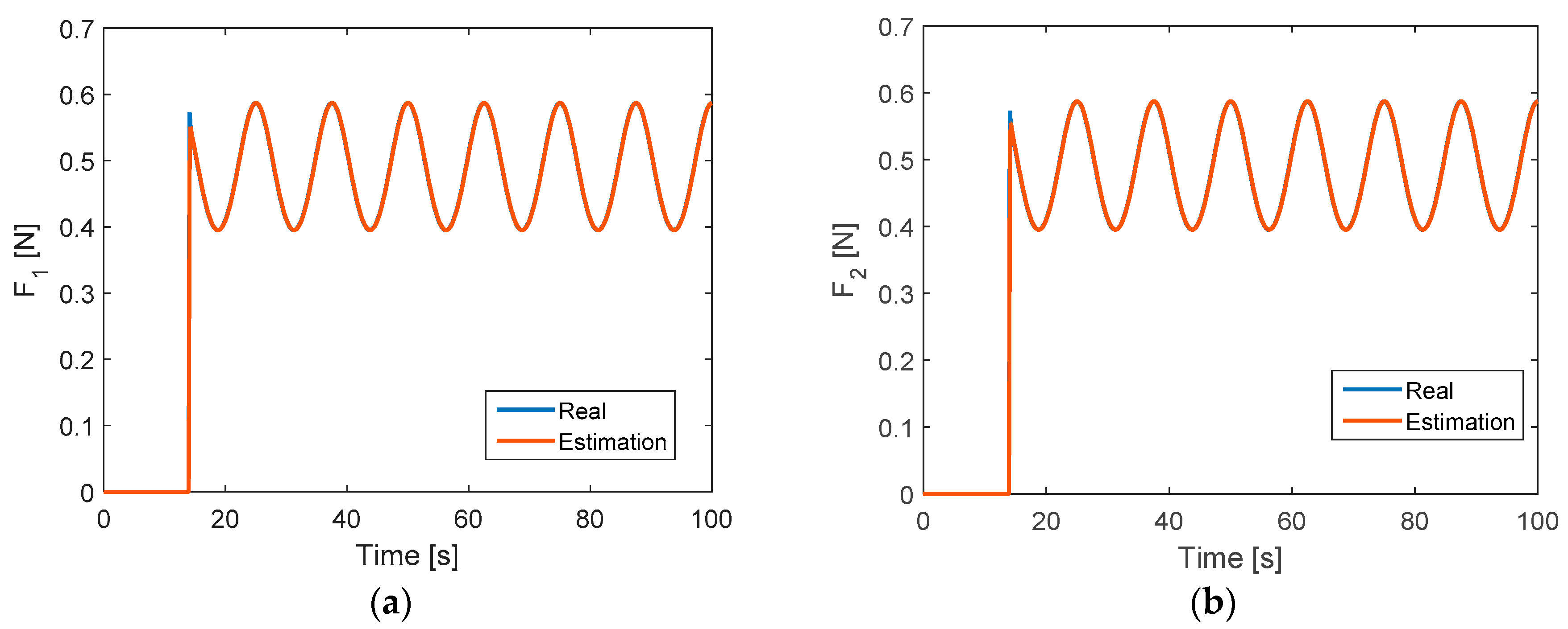
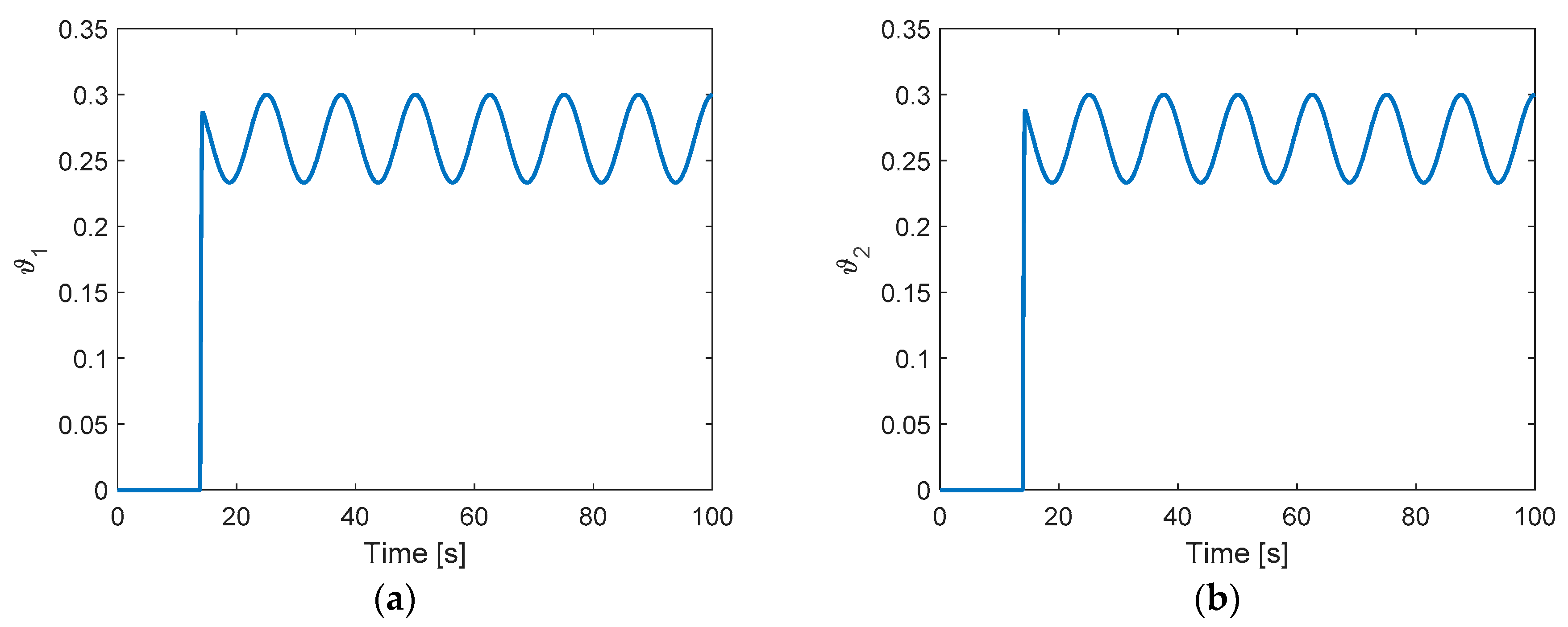
4.1. Fault Diagnosis Results

The parameter of the quadcopter was chosen as shown in

Table 1. Quadcopter parameters.

Parameter	Description	Value
$L$	Arm length	$0.23$ m
$b$	Thrust coefficient	$3.13\times {10}^{-5}$ N/m2
$d$	Drag coefficient	$7.5\times {10}^{-7}$
$m$	Mass	$2$ kg
$I_x;I_y;I_z$	Moments of inertia	$0.0075;0.0075;0.013$ kg·m2
$J_T$	Rotor inertia	$6\times {10}^{-5}$ kg·m2
$K_1,K_2,K_3,K_4,K_5,K_6$	Aerodynamic term	0.01

. The matrices and parameters were chosen for fault diagnosis scheme as follows:

• $P=\left[\begin{array}{cccccccc}1.1035& 0.9849& 0.9853& 0.9848& 0.9859& 0.9853& 0.9851& 0.9852\\ 0.9849& 1.1037& 0.9852& 0.9848& 0.9853& 0.9858& 0.9851& 0.9852\\ 0.9853& 0.9852& 1.1040& 0.9847& 0.9851& 0.9851& 0.9855& 0.9850\\ 0.9848& 0.9848& 0.9847& 1.1038& 0.9854& 0.9854& 0.9852& 0.9859\\ 0.9859& 0.9853& 0.9851& 0.9854& 1.1030& 0.9852& 0.9850& 0.9851\\ 0.9853& 0.9858& 0.9851& 0.9854& 0.9852& 1.1030& 0.9851& 0.9851\\ 0.9851& 0.9851& 0.9855& 0.9852& 0.9850& 0.9851& 1.1033& 0.9856\\ 0.9852& 0.9852& 0.9850& 0.9859& 0.9851& 0.9851& 0.9856& 1.1029\end{array}\right]$;
• $G=\left[\begin{array}{cccc}\mathrm{8,391,000}& -\mathrm{698,000}& -\mathrm{7,032,000}& -\mathrm{4,403,000}\\ -\mathrm{6,980,000}& \mathrm{7,886,000}& -\mathrm{5,560,000}& -\mathrm{6,734,000}\\ -\mathrm{7,032,000}& -\mathrm{5,560,000}& \mathrm{25,348,000}& \mathrm{5,105,000}\\ -\mathrm{4,403,000}& -\mathrm{6,734,000}& \mathrm{5,105,000}& \mathrm{21,777,000}\end{array}\right]$;
• $R_1=\left[\begin{array}{cccccccc}-125.2738& -125.3436& -125.2517& -125.2827& -125.2616& -140.9655& -125.021& -124.74\\ -128.9810& -128.9008& -128.8857& -128.9157& -144.5963& -128.8929& -129.087& -128.37\\ 137.4725& 137.5417& 137.4504& 137.4873& 137.4591& 153.1631& 137.6594& 137.961\\ 133.9164& 133.8360& 133.8182& 133.8564& 149.5312& 133.8278& 133.5907& 134.327\end{array}\right]$;
• $R_2=\left[\begin{array}{cccccccc}\mathrm{431,100}& \mathrm{422,700}& \mathrm{449,600}& \mathrm{451,300}& \mathrm{49,500}& \mathrm{35,000}& \mathrm{477,700}& \mathrm{2,318,200}\\ \mathrm{418,000}& \mathrm{434,400}& \mathrm{448,900}& \mathrm{451,000}& \mathrm{30,400}& \mathrm{59,700}& \mathrm{402,300}& \mathrm{2,422,600}\\ \mathrm{436,100}& \mathrm{440,700}& \mathrm{452,400}& \mathrm{454,000}& \mathrm{55,700}& \mathrm{74,200}& \mathrm{467,900}& \mathrm{1,973,600}\\ \mathrm{438,700}& \mathrm{437,900}& \mathrm{452,000}& \mathrm{454,000}& \mathrm{65,600}& \mathrm{62,100}& \mathrm{420,500}& \mathrm{2,033,700}\end{array}\right]$;
• $\Lambda =0.009I_{4\times 4}$;
• $\rho =1,\epsilon =1$.

The system matrices $A,B,C,H,E_d$ were presented in Section 3.1, and the observer gain matrix was chosen as $L=200I_{8\times 8}$. The parameters were chosen for adaptive sliding mode controller as follows: $k_1=k_2=k_3=0.9$; $A_1=A_2=A_3=10$; ${\beta }_1={\beta }_2={\beta }_3=100$; ${\delta }_1={\delta }_2={\delta }_3=50$.

The sampling time $T=0.001\mathrm{s}$ was chosen for the simulation. The system disturbance was chosen as white noise with the power of 0.005. The trajectory performance of attitude control and altitude control in fault-free operation are shown in Figure 3, where the initial values are ${\varphi }_0=0.1\mathrm{rad}(\approx {5.7}^{°}),{\theta }_0=0.1\mathrm{rad}(\approx {5.7}^{°}),{\psi }_0=0.1\mathrm{rad}(\approx {5.7}^{°}),$ and $z=1\mathrm{m}$. It can be shown that the attitude angles and altitude can converge quickly to the original position.

To test the performance of fault estimation in Equation (12), the initial values were chosen as ${\varphi }_0=0\mathrm{rad},{\theta }_0=0\mathrm{rad},{\psi }_0=0\mathrm{rad},$ and $z=0.5\mathrm{m}$. The time-varying fault offsets were created for motors 1 and 2 as follows:

$${\omega }_{1\_fault}=\{\begin{array}{ll}{\omega }_1,& t<14\left(\mathrm{fault-free}\right)\\ 0.7(1+0.2\sin (2\pi t/25){\omega }_1,& t\ge 14(\left(\mathrm{faulty}\right)\end{array}$$

(50)

$${\omega }_{2\_fault}=\{\begin{array}{ll}{\omega }_2,& t<14\left(\mathrm{fault-free}\right)\\ 0.7(1+0.2\sin (2\pi t/25){\omega }_2,& t\ge 14\left(\mathrm{faulty}\right)\end{array}$$

(51)

The results show that the estimation value converges quickly to time-varying fault offset values with high precision (Figure 4). Figure 5 shows the loss of control effectiveness (LoCE) in each actuator, while Figure 6 and Figure 7 show system states and control inputs. It can be shown that the attitude angles maintain their states in the presence of faults. It is clear that when fault occurs, the roll and pitch motion has more influence than the yaw motion. Therefore, after fault occurs, the altitude is increased to the desired value, although there is a decrease in altitude at the beginning time of fault occurrence.

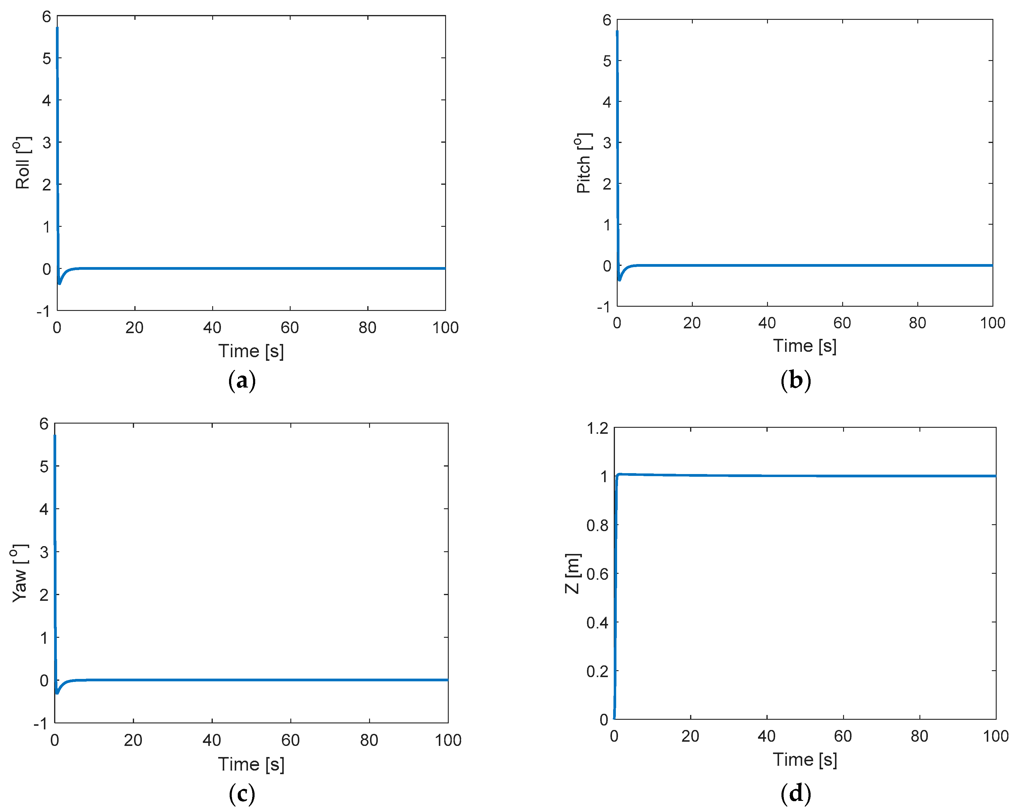
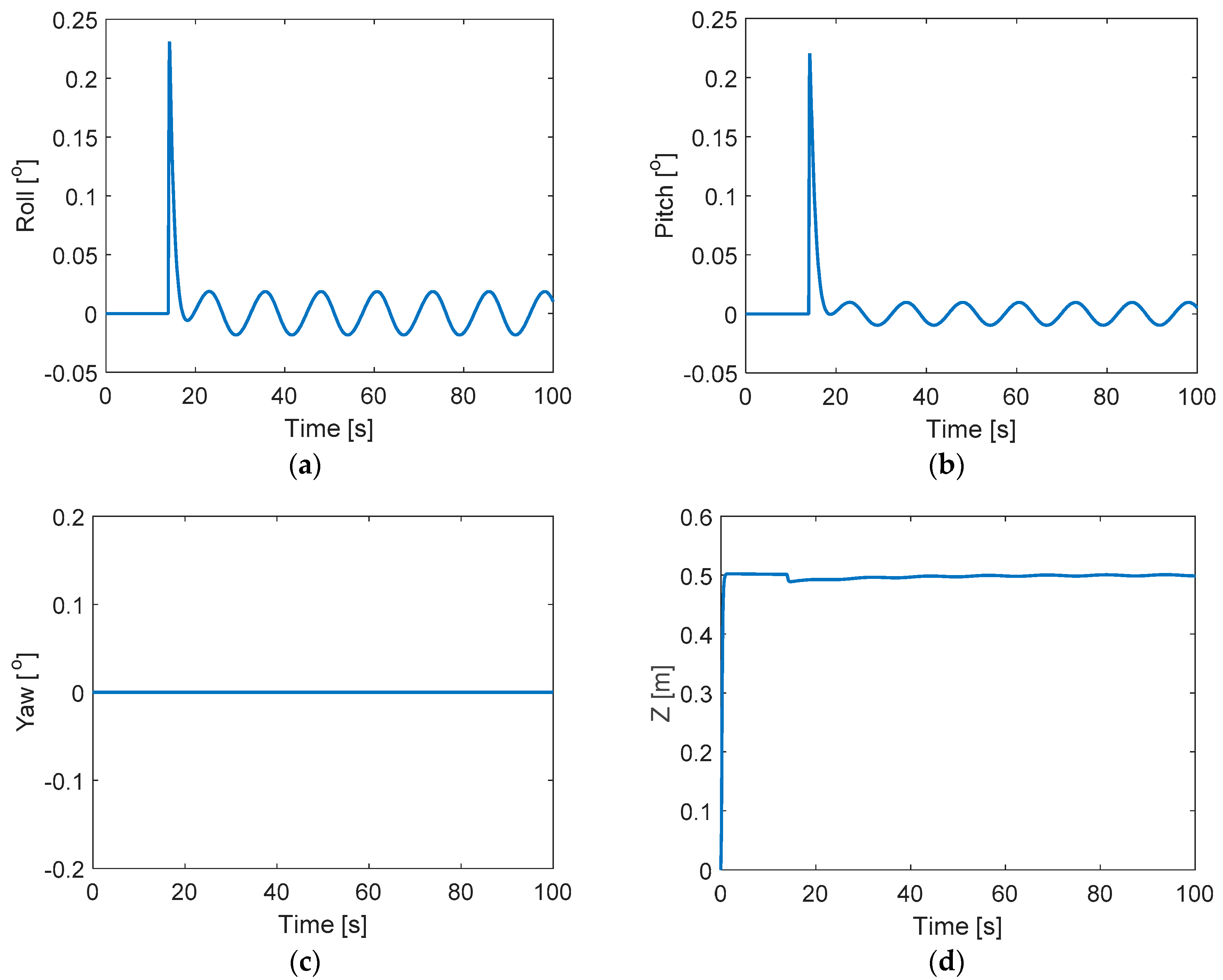
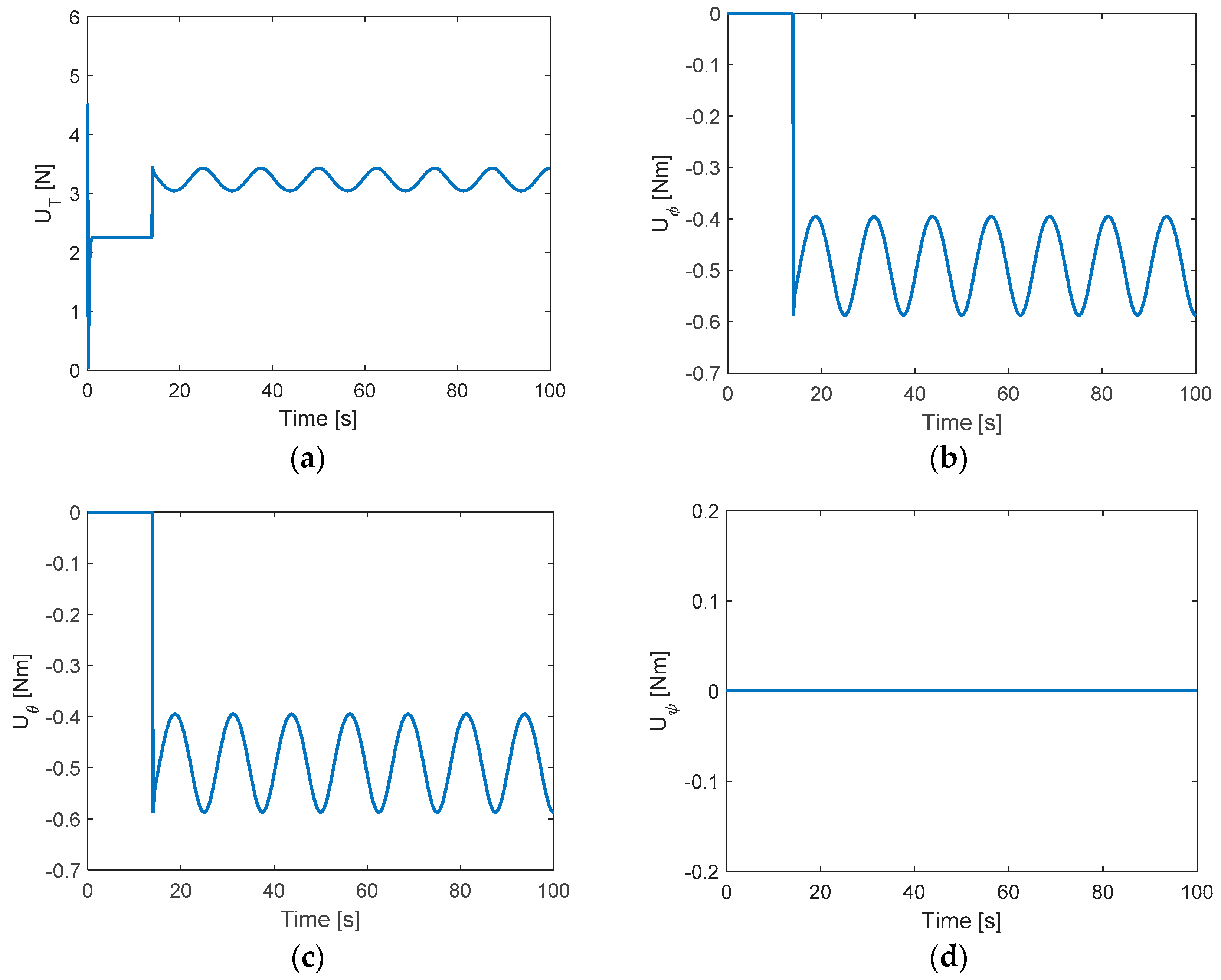
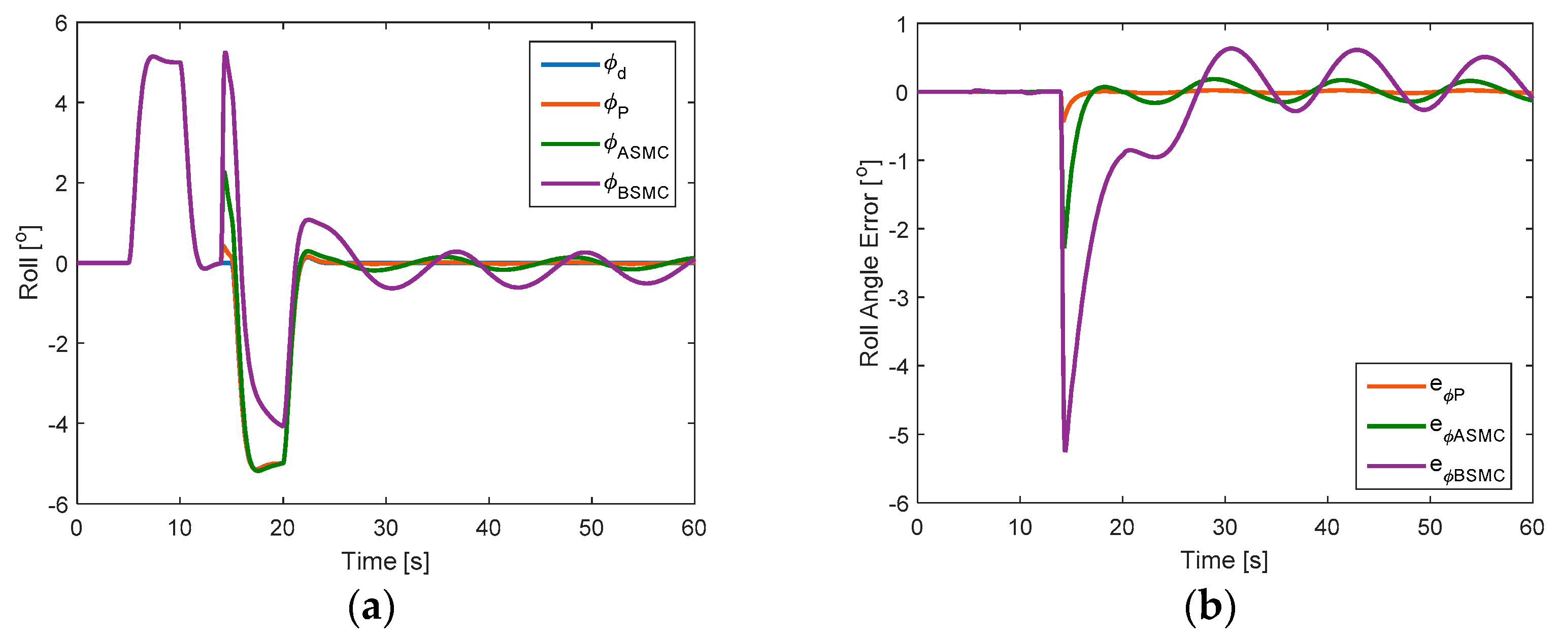
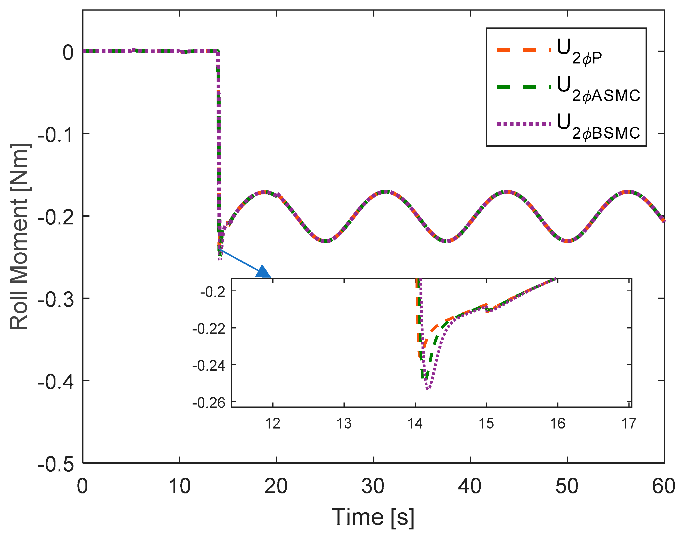
4.2. Active Fault-Tolerant Control Results

The proposed method was compared with the previously proposed robust backstepping sliding mode control (BSMC) [15] and adaptive sliding mode control [44]. In this case, the motion of the quadcopter was designed to converge to the desired roll angle ${\varphi }_d$ in the presence of an actuator fault. The desired roll angle was generated through a filter following Wang et al. [24].

$${\ddot{\varphi }}_d+3{\dot{\varphi }}_d+4{\varphi }_d=4\varphi$$

(52)

where $\varphi$ starts from $0^{°}$, reaches $5^{°}$ at $5$ s, reduces to $0^{°}$ at $10$ s, decreases to $-5^{°}$ at $15$ s, and goes back to $0^{°}$ at $20$ s, and finally, remains at $0^{°}$ for the remaining time.

To demonstrate the effectiveness of MASMBC, a large time-varying fault was injected into actuator 2 with almost 40% LoCE at 14 s as follows:

$${\omega }_{2\_fault}=\{\begin{array}{ll}{\omega }_2,& t<14\\ 0.6(1+0.2\sin (2\pi t/25){\omega }_2,& t\ge 14\end{array}$$

(53)

From the initial time to 14 s, Figure 8 and Figure 9 indicate that all control methods can use the same control torque value and make a good tracking in roll angle and error. In all figures, ${\varphi }_d,{\varphi }_P,{\varphi }_{ASMC},$ and ${\varphi }_{BSMC}$ represent the desired roll angle, actual roll angle using MASMBC, actual roll angle using ASMC, and actual roll angle using BSMC, respectively. When time-varying fault is injected to almost 40% LoCE at 14 s (Equation (53)), the BSMC presents an oscillating performance at the beginning and a low compensation to converge to the desired roll angle. In contrast, MASMBC shows a very good tracking response after a small overshoot at the beginning. The ASMC has a smaller oscillating performance than BSMC, but this method still cannot converge to the desired value.

The MASMBC uses less control effort than ASMC and BSMC when a fault occurs, and there is a similar trend for all controllers after 15 s. Figure 8a indicates that MASMBC offers a quicker compensation in tracking performance than ASMC and BSMC.

It should be noted that by using MASMBC scheme, the tracking error in roll angle can converge quickly to zero after fault occurs (Figure 8b). MASMBC can accommodate faults automatically through fault estimation unit.

The corresponding fault estimation in each actuator is shown in Figure 10. As can be seen, when a fault occurs in actuator 2, the paring actuator 4 is also affected. Moreover, there are some small estimation errors in actuator 1 and 3 when faults occur at 14 s. After 16 s, the fault estimation values converge to zero in actuators 1, 3, and 4.

5. Conclusions

The present study explores the dynamic model of a quadcopter with disturbances and actuator faults. A fault diagnosis scheme is proposed to estimate the magnitude of actuator fault under disturbances. From the fault estimation information, an ASMBC was designed to accommodate the faults and the chattering phenomenon. Then, MASMBC was improved from ASMBC to overcome the input saturations. The results show that MASMBC can offer better tracking performance and quicker compensation than BSMC and ASMC. However, the drawback of this study is that the proposed MASMBC was not verified experimentally. Future work should implement the proposed method on real flight control.

References

1. Yang, S.; Ying, J.; Lu, Y.; Li, Z. Precise quadrotor autonomous landing with SRUKF vision perception. In Proceedings of the IEEE International Conference on Robotics and Automation (ICRA), Seattle, WA, USA, 26–30 May 2015. [Google Scholar]
2. Shakernia, O.; Ma, Y.; Koo, T.J.; Sastry, S. Landing an unmanned air vehicle: Vision based motion estimation and nonlinear control. Asian J. Control 1999, 1, 128–145. [Google Scholar]
3. Zhao, W.; Go, T.H. Quadcopter formation flight control combining MPC and robust feedback linearization. J. Frankl. Inst. 2014, 351, 1335–1355. [Google Scholar]
4. Mahmood, A.; Kim, Y. Decentralized formation flight control of quadcopters using robust feedback linearization. J. Frankl. Inst. 2017, 354, 852–871. [Google Scholar]
5. Nguyen, N.P.; Hong, S.K. Sliding mode Thau observer for actuator fault diagnosis of quadcopter UAVs. Appl. Sci. 2018, 8, 1893. [Google Scholar]
6. Nguyen, N.P.; Hong, S.K. Fault-tolerant control of quadcopter UAVs using robust adaptive sliding mode approach. Energies 2019, 12, 95. [Google Scholar]
7. Ren, W.; Beard, R.W. Trajectory tracking for unmanned air vehicles with velocity and heading rate constraints. IEEE Trans. Control Syst. Technol. 2004, 12, 706–716. [Google Scholar]
8. Bonna, R.; Camino, J.F. Trajectory Tracking Control of a Quadcopter Using Feedback Linearization. In Proceedings of the XVII International Symposium on Dynamic Problems of Mechanics, Natal-Rio Grande Do Norte, Brazil, 22–27 February 2015. [Google Scholar]
9. Tayebi, A.; McGilvray, S. Attitude stabilization of VTOL quadrotor aircraft. IEEE Trans. Control Syst. Technol. 2006, 14, 562–571. [Google Scholar]
10. Madani, T.; Benallegue, A. Backstepping control for a quadrotor helicopter. In Proceedings of the IEEE/RSJ International Conference on Intelligent Robots and Systems, Beijing, China, 9–15 October 2006. [Google Scholar]
11. Raffo, G.V.; Ortega, M.G.; Rubio, F.R. Backstepping/nonlinear control for path tracking of a quadrotor unmanned aerial vehicle. In Proceedings of the American Control Conference, Seattle, WA, USA, 11–13 June 2008. [Google Scholar]
12. Santos, M.; Lopez, V.; Morata, F. Intelligent fuzzy controller of a quadrotor. In Proceedings of the IEEE International Conference on Intelligent Systems and Knowledge Engineering (ISKE), Hangzhou, China, 15–16 November 2010. [Google Scholar]
13. Mardan, M.; Esfandiari, M.; Sepehri, N. Attitude and position controller design and implementation for a quadrotor. Int. J. Adv. Robot. Syst. 2017, 14, 1–11. [Google Scholar] [CrossRef]
14. Xu, R.; Ozguner, U. Sliding mode control of a quadrotor helicopter. In Proceedings of the IEEE Conference on Decision and Control, San Diego, CA, USA, 13–15 December 2006. [Google Scholar]
15. Basri, M.A.M.; Husain, A.R.; Danapalasingam, K.A. Robust chattering free backstepping sliding mode control strategy for autonomous quadrotor helicopter. Int. J. Mech. Mechatron. Eng. 2014, 14, 37–44. [Google Scholar]
16. Yoon, G.Y.; Yamamoto, A.; Lim, H.O. Mechanism and neural network based on PID control of quadcopter. In Proceedings of the 16th International Conference on Control, Automation and Systems, Gyeongju, Korea, 16–19 October 2016. [Google Scholar]
17. Nguyen, T.N.; Lee, S.; Nguyen-Xuan, H.; Lee, J. A novel analysis-prediction approach for geometrically nonlinear problems using group method of data handling. Comput. Methods Appl. Mech. Eng. 2019, 354, 506–526. [Google Scholar]
18. Sharifi, F.; Mirzaei, M.; Gordon, B.W.; Zhang, Y.M. Fault tolerant control of a quadrotor UAV using sliding mode control. In Proceedings of the Conference on Control and Fault Tolerant Systems, Nice, France, 6–7 October 2010; pp. 239–244. [Google Scholar]
19. Xu, D.; Whidborne, J.F.; Cooke, A. Fault tolerant control of a quadrotor using L1 adaptive control. Int. J. Intell. Unmanned Syst. 2016, 4, 1–20. [Google Scholar]
20. Ghandour, J.; Aberkane, S.; Ponsart, J.C. Feedback linearization approach for standard and fault tolerant control: Application to a quadrotor UAV testbed. J. Phys. Conf. Ser. 2014, 570, 082003. [Google Scholar]
21. Chen, F.; Lei, W.; Tao, G.; Jiang, B. Actuator fault estimation and reconfiguration control for the quadrotor helicopter. Int. J. Adv. Robot. Syst. 2016, 13, 1–12. [Google Scholar]
22. Merheb, A.; Noura, H.; Bateman, F. Design of passive fault-tolerant controllers of a quadrotor based on sliding mode theory. Int. J. Appl. Math. Comput. Sci. 2015, 25, 561–576. [Google Scholar] [Green Version]
23. Li, T.; Zhang, Y.; Gordon, B.W. Nonlinear fault-tolerant control of a quadrotor UAV based on sliding mode control technique. In Proceedings of the 8th IFAC Symsosium on Fault Detection, Supervision and Safety of Technical Processes, Mexico City, Mexico, 29–31 August 2012. [Google Scholar]
24. Wang, B.; Zhang, Y.M. Adaptive sliding mode fault-tolerant control for an unmanned aerial vehicle. Unmanned Syst. 2017, 5, 209–221. [Google Scholar] [CrossRef]
25. Fei, J.; Ding, H. Adaptive sliding mode control of dynamic system using RBF neural network. Nonlinear Dyn. 2012, 70, 1563–1573. [Google Scholar]
26. Nicol, C.; Macnab, C.J.B.; Ramirez-Serrano, A. Robust neural network control of a quadrotor helicopter. In Proceedings of the Canadian Conference on Electrical and Computer Engineering, Niagara Falls, ON, Canada, 4–7 May 2008. [Google Scholar]
27. Dierks, T.; Jagannathan, S. Output feedback control of a quadrotor UAV using neural networks. IEEE Trans. Neural Netw. 2010, 21, 50–66. [Google Scholar] [CrossRef] [PubMed]
28. Barghandan, S.; Badamchizadeh, M.A.M.; Jahed-Motlagh, R. Improved adaptive fuzzy sliding mode controller for robust fault tolerant of a quadrotor. Int. J. Control Autom. Syst. 2017, 15, 427–441. [Google Scholar]
29. Modirrousta, A.; Khodabandeh, M. A novel nonlinear hybrid controller design for an uncertain quadrotor with disturbances. Aerosp. Sci. Technol. 2015, 45, 294–308. [Google Scholar] [CrossRef]
30. Nguyen, T.B.; Nguyen, M.H.; Nguyen, A.T.; Dao, P.N.; Nguyen, T.L. Robust H-infinity backstepping control design of a wheeled inverted pendulum system. In Proceedings of the International Conference on System Science and Engineering, Ho Chi Minh City, Vietnam, 21–23 July 2017. [Google Scholar]
31. Kacimi, A.; Mokhtari, A.; Kouadri, B. Sliding mode control based on adaptive backstepping approach for a quadrotor unmanned aerial vehicle. Prz. Elektrotek. 2012, 88, 188–193. [Google Scholar]
32. Cen, Z.; Noura, H.; Younes, Y.A. Systematic fault tolerant control based on adaptive Thau observer estimation for quadrotor UAVs. Int. J. Appl. Math. Comput. Sci. 2015, 25, 159–174. [Google Scholar] [CrossRef]
33. Li, T.; Zhang, Y.; Gordon, B.W. Passive and active nonlinear fault-tolerant control of a quadrotor unmanned aerial vehicle based on the sliding mode control technique. Proc. Inst. Mech. Eng. Part I J. Syst. Control Eng. 2013, 227, 12–23. [Google Scholar] [CrossRef]
34. Alwi, H.; Edwards, C. Fault tolerant control using sliding modes with on-line control allocation. Automatica 2008, 44, 1859–1866. [Google Scholar] [Green Version]
35. Merheb, A.R.; Noura, H.; Bateman, F. Active fault tolerant control of quadrotor UAV using sliding mode control. In Proceedings of the International Conference on Unmanned Aircraft Systems, Orlando, FL, USA, 27–30 May 2014. [Google Scholar]
36. Fortuna, L.; Frasca, M. Optimal and Robust Control—Advanced Topics with Matlab; CRC Press: Boca Raton, FL, USA, 2012. [Google Scholar]
37. Amoozgar, M.H.; Chamseddine, A.; Zhang, Y. Experimental test of a two-stage Kalman filter for actuator fault detection and diagnosis of an unmanned quadrotor helicopter. J. Intell. Robot. Syst. 2013, 70, 107–117. [Google Scholar]
38. Xuan-Mung, N.; Hong, S.-K. Improved Altitude Control Algorithm for Quadcopter Unmanned Aerial Vehicles. Appl. Sci. 2019, 9, 2122. [Google Scholar] [Green Version]
39. Nguyen, A.T.; Xuan-Mung, N.; Hong, S.-K. Quadcopter Adaptive Trajectory Tracking Control: A New Approach via Backstepping Technique. Appl. Sci. 2019, 9, 3873. [Google Scholar] [CrossRef]
40. Xuan-Mung, N.; Hong, S.K. Robust adaptive formation control of quadcopters based on a leader–follower approach. Int. J. Adv. Robot. Syst. 2019, 16, 1–11. [Google Scholar]
41. Nguyen, N.P.; Hong, S.K. Fault Diagnosis and Fault-Tolerant Control Scheme for Quadcopter UAVs with a Total Loss of Actuator. Energies 2019, 12, 1139. [Google Scholar] [CrossRef]
42. Nguyen, N.P.; Hong, S.K. Robust Fault Diagnosis for a Quadrotor with Actuator Fault. I. J. Engineer. Technol. 2018, 7, 74–77. [Google Scholar]
43. Nguyen, N.P.; Hong, S.K. Position control of a hummingbird quadcopter augmented by gain scheduling. Int. J. Eng. Res. Technol. 2018, 11, 1485–1498. [Google Scholar]
44. Nadda, S.; Swarup, A. On adaptive sliding mode control for improved quadrotor tracking. J. Vib. Control 2017, 24, 3219–3230. [Google Scholar] [CrossRef]
Figure 1. Quadcopter configuration.
Applsci 09 04010 g001
Figure 2. Control structure of a quadcopter.
Applsci 09 04010 g002
Figure 3. Trajectory performance of attitude and altitude control in fault-free operation: (a) Roll angle; (b) Pitch angle; (c) Yaw angle; (d) Altitude.
Applsci 09 04010 g003
Figure 4. Fault estimation in the presence of white noise: (a) F1 fault offset; (b) F2 fault offset.
Applsci 09 04010 g004
Figure 5. Loss of control effectiveness of actuators: (a) actuator 1; (b) actuator 2.
Applsci 09 04010 g005
Figure 6. System states in the presence of faults: (a) Roll angle; (b) Pitch angle; (c) Yaw angle; (d) Altitude.
Applsci 09 04010 g006
Figure 7. Controller inputs: (a) Thrust; (b) Roll moment; (c) Pitch moment; (d) Yaw moment
Applsci 09 04010 g007
Figure 8. Comparison of tracking performance between modified adaptive sliding mode backstepping control (MASMBC), adaptive sliding mode control (ASMC), and backstepping sliding mode control (BSMC): (a) Roll angle; (b) Tracking error.
Applsci 09 04010 g008
Figure 9. Comparison of control torque between MASMBC, ASMC, and BSMC with 40% loss of control effectiveness (LoCE) in actuator 2.
Applsci 09 04010 g009
Figure 10. Fault estimation in the presence of white noise: (a) actuator 1; (b) actuator 2; (c) actuator 3; (d) actuator 4.
Applsci 09 04010 g010