Abstract
To avoid stick-slip vibration, one of the most important forms of self-excited vibrations in deep hole drilling, this paper studies the stability and bifurcation characteristics of a drilling system based on a two-degree-of-freedom discrete model. It is a state-dependent delay model that could describe the non-linear dynamic characteristic of drilling systems more accurately, compared with the traditional constant delay models. In this paper, linear stability analyses of both the state-dependent delay model and the traditional constant delay model are carried out. Hopf bifurcation analyses are then performed by the method of multiple scales. The results show that the state-dependent delay model can provide more precise stability boundaries and more desirable supercritical Hopf bifurcation properties compared to the constant delay model. The control parameters (rotational velocity and feed velocity) will affect these results. It is noted that the method is reliable for deep hole drilling stability prediction and can provide a reference for dynamic optimization design.
1. Introduction
Delay differential equations (DDEs) often appear in various fields of science and engineering, such as control systems [1], lasers [2], neuroscience [3] and cutting process dynamics. For cutting dynamics, the cutting effect of tools can cause vibrations in the cutting system, resulting in accelerated wear of tools and influencing the cutting process in machines (turning, milling and grinding), coal seam mining, geological prospecting and oil drilling.
Tobias [4] proposed the theory of regenerative cutting of the tool. During the cutting process, the cutting thickness of the workpiece is constantly changing due to the relative vibration of the tool and the workpiece. The cutting force of the cutter is a function of cutting thickness and depends on the tool’s current and delay position. This theory has been widely accepted as the basis for cutting theory and experimental research.
This paper mainly studies the non-linear dynamic stability of the deep hole drilling in coal seam gas exploitation (see Figure 1). Mine gas extraction is an important guarantee of safety and efficiency in coal mining. However, the drilling process can lead to strong self-excited vibration, which will affect the drilling stability. The self-excited vibration in drilling is similar to the chatter vibration in the cutting; both are caused by the regenerative cutting of the tool or drill bit.
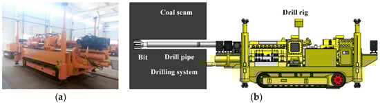
Figure 1.
Deep hole drilling in coal seam gas exploitation: (a) Deep drill rig; (b) 3D model.
There are three types of self-excited vibration of drill string, axial vibration, torsional vibration and lateral vibration. They can lead to bit bounce, stick-slip and bit whirl, respectively [5]. These vibrations can affect the stability of machines and the drill string could be broken when the frequency of self-excited vibration is close to the natural frequency of the system. To avoid these vibrations and improve the drilling efficiency, the specific conditions need to be studied. Leine [6,7] contrasted the bifurcation phenomenon of the stick-slip model, the whirl model, and the stick-slip whirl model at the equilibrium point of the drilling system in oil drilling and found that the whirl had a certain influence on the stick-slip, mainly due to the existence of fluid force in drilling. However, the effect of fluid force is not so obvious in directional drilling due to the different drilling’s structures. Liao [8,9,10] analyzed the influence of whirl on the frequency components and the motion law of the axis trajectory of the drilling system by establishing a drilling test bed. However, the research was more biased towards the rubbing of rotor and stator, and could not really reflect the cutting motion of the drill bit.
In fact, the regenerative cutting motion of the bit is the main cause of the system vibration, which is determined by the axial feed and torsional speed of the drilling system. Germay [11] used singular perturbation analysis to decouple axial and torsional dynamics in the model, and then conducted a detailed analysis of the axial limit cycle ensuring drilling outside of an unstable region. Besselink [12] considered the axial damping in Germay’s model and analyzed the effect of axial periodic motion by a semi-analytical method. The results of the literature have confirmed that the influence of axial vibration on stick-slip vibration cannot be ignored. On the other hand, stick-slip was observed at low rotational velocity and high feed velocity of the bit [13,14], while bit whirl occurred at high rotational velocity and low feed velocity [15,16]. So, stick-slip vibration is the main form of self-excited vibrations for deep hole drilling with low rotational velocity and high feed velocity [17].
Kovalyshen [18] and Richard [17] specifically described stick-slip vibration that was characterized by alternate stick and slip phases. In a stick phase, the bit stops and the drill pipe continues to twist. In a slip phase, the rotational velocity of the bit increases instantly because of the energy stored by the drill pipe in the stick phase. This phenomenon would periodically change stress and strain to accelerate the fatigue failure of the drilling system.
The most common stick-slip model used in the present study is non-linear, including material non-linearity [19] as well as structural non-linearity [20]. The effect of cutting force is the largest among all the non-linear factors [21,22]. Hanna and Tobias [23] proposed a non-linear cutting model that included non-linear stiffness and non-linear cutting force. Kovalyshen [17] considered non-linear contact stress in the drilling process. These studies have shown that the non-linear factors have a significant impact on system stability. Shi and Tobias [24] pointed out the non-linearity of a drilling system is mainly caused by the non-linear cutting force. Their study was supported by subsequent experimental research.
The factors of the non-linear cutting force are mainly reflected in the changing delay time. However, the most commonly delay model used in previous studies is the linear constant delay (CD) model, which is equal to the period of the drill bit (workpiece) rotation in drilling (turning, milling). The mathematical model is usually an autonomous delayed differential equation with constant delay (CD-DDE). Models with constant time delay capture the main characteristics of regenerative dynamics, but these models can only be applied in linearized systems. When the system is non-linear, the calculated results cannot be in good agreement with the experiments.
Recently, the concept of non-linear state-dependent delay (SDD) was presented [25,26]. Long [27] and Balachandran [28] pointed out that the regenerative delay was time-dependent due to the feed rate in an accurate model of the milling process. They showed that the traditional constant delay models overestimate stability limits for large feed rates. The regeneration of delay in the turning system is mainly determined by the workpiece’s speed, but also affected by the current and delay position of the tool. This is the state-dependency delay (SDD) model, and the mathematical model is a delayed differential equation with state-dependent delay (SD-DDE).
The SD-DDE is an autonomous non-linear equation and its solution is non-differentiable due to the state-dependent time delay , as shown in Equation (1). CD-DDE can be considered a linear variational system, corresponding to Equation (1) at the equilibrium point , as shown in Equation (2). Therefore, the analysis of a drilling system represented by a SD-DDE is more complicated than the conventional constant DDE (C-DDE). Richard [29,30] investigated drilling with drag bits and found that state-dependent regenerative delay arose due to the torsional vibration of the tool. For deep hole drilling, the effect of state-dependent delay is especially apparent.
In order to study the influence of non-linear state-dependent delay on deep hole drilling systems, this paper studied and compared the stability of CD and SDD models through the lobes diagram. On the other hand, control parameters (rotational velocity and feed velocity) could be chosen to ensure a stable cutting process without stick-slip vibration based on the lobes diagram. The non-enclosed stability lobes diagram is a function of axial cutting depth on spindle speed, which can be drawn using numerical or semi-analytic methods [31,32,33,34,35].
Recently, Liu and Balachandran [36,37] carried out a stability analysis using a semi-discretization and constructed a stability volume in the three-dimensional parameter space of spin speed, cutting depth and a cutting coefficient. They used a two degree-of-freedom model and a multisegment model of drill strings with state-dependent delay. Nandakumar [38] plotted the stability charts in the plane of drilling rates and rotary speeds. In order to understand the root cause of stick-slip vibrations in deep drilling, Kovalyshen [17] analyzed the stability of the following three cases: (i) the case of negligible torsional compliance (pure axial vibrations); and (ii) the case of negligible axial compliance (pure torsional vibrations); (iii) the general case of coupled axial–torsional vibrations. Results showed the axial vibration of drill-string systems play a key role in stabilizing the torsional vibration. However, the studies were based on the state-dependent delay model and did not indicate the differences in stability of the constant delay model and state-dependent delay model.
On the other hand, a stable cutting state can also cause vibrations due to Hopf bifurcation, which accompanies stick-slip vibration. For turning models with constant delay, subcritical Hopf bifurcations occur, i.e., unstable periodic orbits coexist with the stable stationary cutting below the stability lobes. This means that chatter may arise in cases where the system is linearly stable. This phenomenon was clearly shown by Inspergera [16]. Therefore, it is necessary to carry out Hopf bifurcation analysis on the deep hole drilling system.
In this paper, a two-degree-of-freedom model considering axial and torsional vibration was established, and the linear stability and the characteristics of Hopf bifurcation of the drilling system were studied by using the method of multiple scales. The results of the constant model and state-dependent delay model were analyzed to find the most appropriate control parameters and avoid stick-slip vibration.
2. Dynamic Model of Drilling System
2.1. Dynamic Equations of Drilling System
In deep hole drilling, the vibration of the system mainly refers to the vibration of the drill bit and the drill pipe, which could also be called a drilling system (see Figure 1b). The rotational velocity Ωrot and feed velocity decided by the rig are the most important control parameters in deep hole drilling. After establishing the dynamic model, the output characteristic of the drill bit at any time could be analyzed by the geometric structure of the drill, the rock characteristics, and the rock breaking mechanism of the drill bit, i.e., the actual drilling speed V and rotating speed Ω of the drill bit. Also, the control parameters could be changed to achieve the desired output characteristics of the drilling system and avoid stick-slip vibration, which is the purpose of this paper.
The stick-slip vibration frequency is similar to its torsional vibration frequency of the drilling system through test analysis and field observation. On the other hand, the axial drilling speed and torsional rotational speed can directly affect the drilling process of the drill bit. So a discrete model of the drilling system is characterized by two degrees of freedom, Z and Φ, corresponding to the axial and angular position of the bit, respectively. This model has six mechanical elements from Table 1, namely point mass m, moment of inertia I, torsional stiffness KT and axial stiffness KA, torsional damping and axial damping (see Figure 2). The mass m and the moment of inertia I are taken to represent the bit, while the spring K and the damper are assumed to stand for the drill pipe. The drilling system is affected by two boundary conditions, the input of the drill rig (constant input drilling speed and rotational speed ) and the bit-coal interaction (the bit weight W and torsion T of the drill bit).

Table 1.
Parameters in the discrete model.
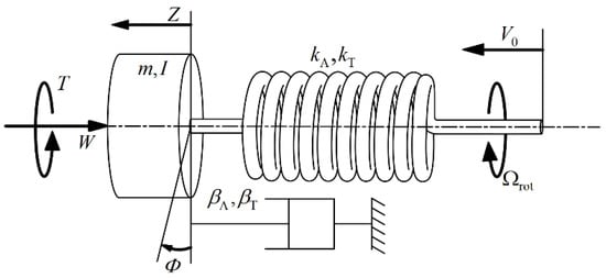
Figure 2.
Dynamic model of the drill string system.
The perturbation dynamic equations of the drilling system can thus be written in the form:
where are the disturbed axial displacement and angular displacement under stable drilling of the drilling system. and are the non-linear disturbance cutting force, which is determined by the nature of the coal, the structure of the drill and the depth of the cutting depth, i.e., the difference between the instantaneous cutting force and steady-state cutting force at any time of the drilling system.
The PDC (Polycrystalline Diamond Compact) bit is widely used in deep hole drilling in coal seam with good impact toughness and the ability to handle minor accidents. According to the single blade cutting experiment of PDC bit [18], the action of such a bit consists of two independent processes, i.e., a cutting process taking place on the cutting face and a frictional contact process taking place on the wearflat. So, we can synthesize the bit-rock interaction into bit weight W and torsion T, see Figure 3 and the disturbance cutting force could be written as follows:
where ζ and s are the parameters that characterize the angle of cutter and the coal properties, a is the radius of the bit, N is the identical blades number of bit, d and are the instantaneous and stable cutting depth per revolution of the drill bit, respectively. The axial displacement of bit from time to time t is d(t) in Figure 4. and are the axial and torsional position of the bit at time t.
where . is a state-dependent delay time required for the bit to rotate an angle 2π/N to its current position at time t and determined by the following equation:
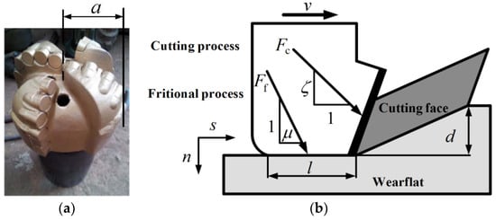
Figure 3.
PDC bit in deep hole drilling: (a) The PDC bit; (b) single blade cutting model.
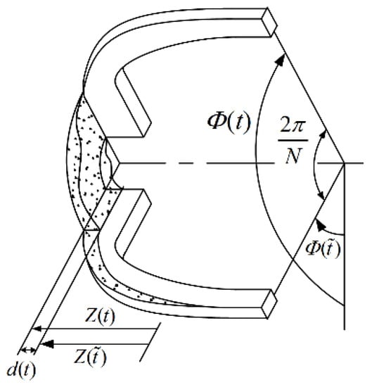
Figure 4.
The profile located between two successive blades of a PDC bit.
The spatial location at any time of the drill bit can be expressed as:
The cutting depth can be obtained by Equations (7)–(9), which is calculated by the delay time and disturbed value:
On the other hand, the delay time of the drilling system can be sorted into Equation (12), which is a function determined by time and torsional state, called state-dependent delay (SDD). It is also possible to see the importance of torsional vibration of the drilling system through the form of SDD. At the same time, we can simplify the SDD into a constant delay (CD), as follows:
Then the SDD model Equations (14) and (15) and CD model Equations (16) and (17) can be obtained by the substitution of Equations (5), (6) and (10)–(13) into the perturbation dynamic equations, respectively.
where .
It is worth noting that the drilling system will have a bit bounce and the drill bit will be separated from the coal when d < 0. So the analysis is based on d > 0 in this paper.
2.2. Scaling
The stick-slip vibration is essentially for the development of the torsional vibrations. So the torsional natural frequency of the drill string is used to simplify the time scale and the torsional rigidity is used to simplify the axial cutting depth. In order to describe the influence of control parameters on the drilling system, a control parameter ρ was defined. For deep hole drilling, these control parameters are from Table 2.
Table 2.
Control parameters of the deep hole drilling.
Using Equation (18) to simplify the SDD, CD model:
where
Parameter is the dimensionless delay time, ωA is the natural frequency of the axial vibrations, and are the axial and torsional amplification factors, respectively. The parameter kr characterizes the torsional stiffness and bit structure. The parameters used in the numerical studies are . The dimensionless rotational speed Ω is usually less than 5 () and the parameter is less than 1 ().
2.3. Taylor Series Expansion of the Nonlinear Cutting Force
Stability analysis of system with state-dependent delay is more complicated than the system with constant time delay, because the solution of the system is non-differentiable. At the same time, the traditional numerical method cannot be used directly due to the implicit form of the state-dependent delay. The SDD model cannot be completely linearized. So a linear differential equation needs to be sought that has a common dynamic characteristic with SDD. Hartung and Turi [39] linearized the regular SD-DDEs, Hartung [40] linearized the SD-DDEs of the time period. In this paper, the Taylor series was used to linearize the implicit SDD.
To analyze the Hopf bifurcation characters in the SDD and CD model of the drilling system, the implicit SDD was successfully converted into an explicit form through a series of expansion procedures. Assuming that small displacement disturbances ξ and η occur in the z and directions of the drilling system, respectively, and the displacements in the dynamic equations can be expressed as:
The series expansion for the SDD at the equilibrium point () can be expressed as [41]:
where is a small, positive parameter, .
Substitution of Equations (25) and (26) into Equations (20) and (21) yields:
Defining a state vector and rewriting the equations in vector form:
The state vector equation of the CD model is:
where the coefficient matrices and the non-linear forcing vector are given in Appendix A.
3. Linear Stability Analysis
The dynamic equations of the drilling system (Equations (14)–(17)) have a stable solution, i.e., (drilling without vibration), which is the equilibrium point of the system. The stability of the equilibrium point is analyzed in this section. The linearized homogeneous state vector equation can be obtained from Equations (30) and (31) as:
This is a delayed differential equation, and its characteristic equation is:
where λ denotes an eigenvalue of the linearized system and the exponential term appears due to the time delay.
There are an infinite number of eigenvalues in Equation (33). The drill string system is stable only when all the eigenvalues have negative real part , otherwise the system is unstable. Pure imaginary eigenvalues corresponding to a specific condition determine the stability boundaries that divide the stable and unstable regions. In this case, the responses of the drilling system exhibit periodic oscillations with frequency .
Assuming that the eigenvalue λ is equal to , the characteristic Equation (33) could be converted into a frequency equation, and the following four equations can be obtained by separating the real part and imaginary part. Using as the parameter, the stability diagrams of the SDD model and CD model, respectively, could be drawn (see Figure 5). The abscissa is the non-dimensional rotational speed Ω and the ordinate is the non-dimensional axial cutting depth ψ.
where k = 1, 2, 3, …, and represents the number of lobes.
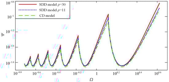
Figure 5.
Stability charts of SDD and CD model.
There are seven lobes in the Figure 5; the upper part of the lobe is the instability of the drilling system, the lower part of the lobe is the stable interval, and the lobe represents the critical cutting depth. In the case of drilling, the appropriate control parameters Ω and ρ can be chosen through the stability lobes to realize a working condition without stick-slip vibration and improve drilling efficiency. From the figure, it can be seen that the system stability interval increases with non-dimensional rotational speed. On the other hand, the stability boundaries are higher for the state-dependent delay model than for the constant delay model. For the SDD model, the system stability interval increases with the control parameters ρ.
In order to make a more intuitive analysis of the change law of the critical cutting depth with the rotation speed of the SDD and CD model, 3D waterfalls (Figure 6) were drawn. These figures are the change law of the critical non-dimensional cutting depth ratio of the first lobe and the seventh lobe, respectively. The Z-axis is the critical non-dimensional cutting depth ratio between the SDD and CD model (), the X-axis is the control parameter ρ, and the Y-axis is the vibrational frequency . From the figure, it can be seen that the critical non-dimensional cutting depth ratio increases with the increase of control parameter ρ and vibrational frequency , the maximum can reach 1.1. Comparing the two figures, the change law of the critical non-dimensional cutting depth ratio is consistent in each lobe and there is no significant difference. On the other hand, the ratio is small (closer to 1) in the case of small control parameters, but the value of critical non-dimensional depth ratio increases significantly with the variation of vibrational frequency .
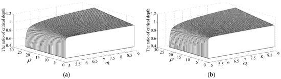
Figure 6.
The change law of the critical dimensionless cutting depth ratio of SDD and CD model: (a) the first lobe; (b) the seventh lobe.
In order to verify the accuracy of the stability lobes diagram, three points A, B and C at the Ω = 2 on the lobe graph are chosen. The coordinates are A (2, 0.01), B (2, 0.03) and C (2, 0.0234), respectively. A is located in the stable cutting region, with B in the unstable cutting region. For SDD model, point C is located at the stability boundary when ρ = 11. The perturbation axial velocity and perturbation torsional velocity at A, B and C of the two models were solved by the Runge-Kutta numerical algorithm, as shown in Figure 7, Figure 8 and Figure 9, where the parameter value is v = 0.1, kr = 10, QA = QT = 5, N = 4.
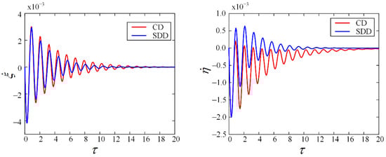
Figure 7.
Evolution with time of responses for the CD model and SDD model at point A.
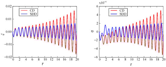
Figure 8.
Evolution with time of responses for the CD model and SDD model at point B.
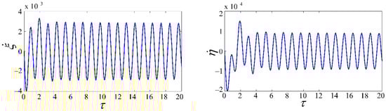
Figure 9.
Evolution with time of responses for the SDD model at point C.
At point A, the responses of the two models are significantly attenuated. There is no significant difference in axial velocity between the two models. However, the SDD model has greater torsional speed amplitude because the state-dependent delay depends not only on the time but also on the system’s torsional state. At point B, the torsional speed of the two models increases dramatically with time and the system is extremely unstable. When the disturbance torsional speed is equal to the amplitude of the system input rotational speed, the system enters the stick-slip state. At point C, the SDD model developed into periodic motion after 4 s, and the axial and torsional phase diagrams show a strict limit cycle state, as seen in Figure 10.
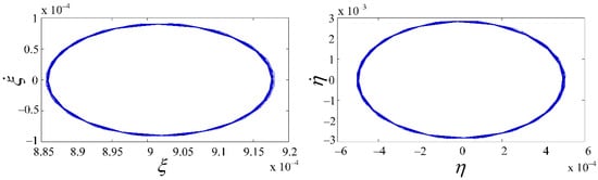
Figure 10.
The axial and torsional phase diagram of the SDD model.
The above numerical results show that the stability lobes diagram can accurately predict the stable and unstable cutting area of the drilling system at Ω = 2. However, at a certain speed, this prediction is less accurate due to the existence of Hopf bifurcation. Therefore, the Hopf bifurcation area of the drilling system is solved in this paper.
4. Resolving Process of Method of Multiple Scales
The method of multiple scales (MMS) is the most representative for solving the stable periodic responses of non-linear delay differential equations (DDEs). The non-linearity of such systems is very small. Therefore, it is possible to take non-linear factors as perturbations of a linear system, and then find the approximate solution of a non-linear system on the basis of a linear system. The Taylor approximation and small parameterization of non-linear delay time have been performed in this paper.
Different time scales for SDD model and the time-variable functions of different scales are treated as independent variables. The derivative of the response with respect to time can be expanded by the power of .
with , which is a partial differential operator.
Non-linear process can be expressed as the function of different scales of time, this article only consider time variables to simplify calculation. The periodic solution and delay solution of the state vector Equation (30) in the Hopf bifurcation point is expand to the second order of :
where is the nth order periodic function of the time scales .
To satisfy the continuity requirement of Equation (44), the axial depth of cut is set to be a sum of the linear critical depth of cut and the perturbed depth of cut as:
By substituting Equations (42)–(46) into Equation (30) and equating the coefficients of like powers of ε, the differential equations with the zeroth, first and second orders of ε can be obtained:
where , are the coefficient matrices of the current and delayed state vectors with the linear critical depth of cut, respectively. are the coefficient matrices of the current and delayed state vectors with the perturbed depth of cut, respectively. and are the first- and second-order functions of the non-linear forcing vector shown in Equation (31) (see Appendix B.1).
Equation (48) did not contain a secular term, so, . Researching the system responses near the Hopf bifurcation point, the solution of the zero order approximation equation is written as the plural form:
where is the linear vibrational frequency at the Hopf bifurcation point, and are the eigenvectors associated with the eigenvalues , and are a pair of undetermined conjugated complex functions.
The substitution of Equations (50) and (51) into Equation (48) yields the particular solution of the non-homogeneous differential equation in the form:
where are described in detail in Appendix B.2.
Substitution of Equations (50)–(52) into Equation (49) yields:
where and are the coefficient vectors for the complex harmonic terms originating from (see Appendix B.3). c.c. is the conjugate term of its previous term.
To avoid secular term, we get an equation for A1, where and are real constants given in Appendix B.4:
We introduce the polar form amplitudes:
where and are the amplitude and phase of the drilling system.
Substituting (55) into (54) and separating the real and imaginary parts of the resulting equation, the first order bifurcation equation of the amplitude and in real form can be obtained as:
For periodic motion, , the bifurcation solution of drilling system amplitude and phase can be obtained by:
The stable periodic motion near the Hopf bifurcation point is subcritical when the sign of both and are the same; otherwise it becomes supercritical.
The second equation of (Equation (46)) is reduced to:
Substitution of Equations (50)–(52) into Equation (55) yields:
where is given in Appendix B.5.
Finally, the quadratic approximation of the drilling system in the Hopf bifurcation point is:
5. Hopf Bifurcation Analysis
In actual drilling, self-excited vibration system will be associated with the Hopf bifurcation dynamic phenomenon. So the stable cutting zone is not well judged by the system linear stability analysis. Hopf bifurcation refers to the phenomenon whereby the equilibrium point is changed from stable to unstable and form limit cycles when the system parameter changes pass a critical value. It is closely related to the production of self-excited vibration in engineering. The self-excited vibration with Hopf bifurcation will cause instability in the drilling system. The limit cycle exists when the value of bifurcation parameter is less than the threshold and it is the subcritical Hopf bifurcation. Otherwise it is supercritical Hopf bifurcation.
The Hopf bifurcation feature is shown in Figure 11; the amplitude of the drilling system is a function of axial dimensionless cutting depth . The linear stability boundary of the drilling system is ; the cutting of system is stable when , otherwise it is unstable. In a subcritical case, when an unstable limit cycle (periodic orbit) coexists with the stable equilibrium (stationary cutting), the system may produce stick-slip vibration. In a supercritical case, a stable limit cycle coexists with the unstable equilibrium, so the system is stable.
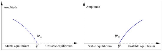
Figure 11.
Sketch of subcritical and supercritical Hopf bifurcations.
5.1. Hopf Bifurcation for the Constant Delay Model
Figure 12 shows the change of the Hopf bifurcation to the stability lobes of the constant delay model; the blue line represents the sub-critical Hopf bifurcation area. It can be seen that the system only has the subcritical Hopf bifurcation in the case of the constant delay model because it is mainly related to the dependence of the non-linear cutting force on the cutting thickness.
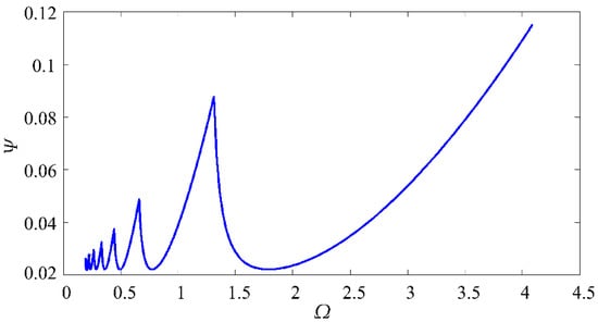
Figure 12.
The change of Hopf bifurcation to stability lobes of the CD model.
To verify the Hopf bifurcation feature of the constant delay model, the variation of amplitude a and axial dimensionless cutting depth were plotted at Ω = 1.2, 2, 4; ρ = 11 (see Figure 13, Figure 14 and Figure 15). It can be seen that the amplitude of the drilling system will continue to increase until it loses stability (sharp point) in the stable cutting area. Therefore, the linear stability region of the drilling system is unstable and may be self-excited.
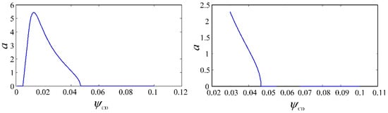
Figure 13.
The variation of the amplitude a with the dimensionless cutting depth (Ω = 1.2, ρ = 11).
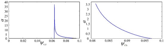
Figure 14.
The variation of the amplitude a with the dimensionless cutting depth (Ω = 2, ρ = 11).
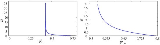
Figure 15.
The variation of the amplitude a with the dimensionless cutting depth (Ω = 4, ρ = 11).
5.2. Hopf Bifurcation for State-Dependent Delay Model
Figure 16 shows the change of the Hopf bifurcation to the stability lobes of the state-dependent delay model with different values of control parameter . The blue line represents the subcritical Hopf bifurcation area and the red line represents the supercritical Hopf bifurcation area. In Figure 16, Hopf bifurcation does not change the entire stability lobes. It can be seen that the right side of the lobes becomes supercritical with the increase of , while the left side does not change. The drilling system has only supercritical Hopf bifurcation in the low rotational speed region (Ω < 0.5).
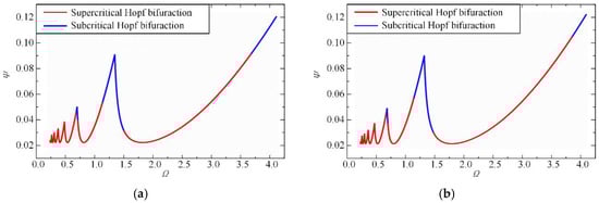
Figure 16.
The change of Hopf bifurcation to stability lobes of the SDD model: (a) ρ = 11; (b) ρ = 30.
In the subcritical Hopf bifurcation section, there is a stable periodic motion when drilling in a linear unstable region and the system’s linear stability region does not have unstable periodic motion. This means that stick-slip vibration will not occur in the system when the stability parameter axis cutting depth is over a certain threshold. The periodic vibration occurs in the drilling system only when it loses stability, and the amplitude of stick-slip vibration increases with . Therefore, in the supercritical Hopf bifurcation section, the system will not become unstable. Under practical conditions, the supercritical Hopf bifurcation is more advantageous than the subcritical Hopf bifurcation.
Figure 17 shows the change of the control parameters ρ to the Hopf bifurcation properties (a) and the critical control parameters ρ of the Hopf bifurcation at different rotational speeds Ω (b) in the first stability lobe (1 < Ω < 4.5). In order to study the limit of deep hole drilling, we extend the range of ρ to twice the rated working condition (ρ ≤ 70). It can be seen from the figure that no matter how ρ changes, the bifurcation properties of the drilling system will not change in the non-dimensional rotational speed range 1–3.5. Only when the non-dimensional rotational speed is greater than 3.5 will the subcritical Hopf bifurcation be converted into the supercritical Hopf with the increase in ρ. In actual drilling, the corresponding control parameters can be selected according to Figure 17, and the system is in the zone of supercritical Hopf bifurcation, which can ensure the stability of the drilling system.
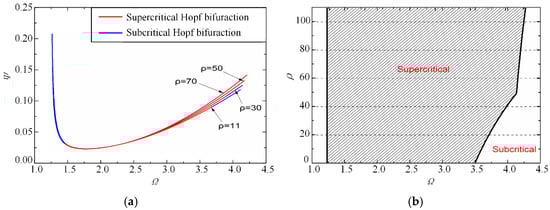
Figure 17.
Change of criticality along the first stability lobe of SDD model (1 < Ω < 4.5): (a) Change of the control parameters ρ to the Hopf bifurcation properties; (b) change of the critical control parameters ρ of the Hopf bifurcation at different rotational speeds Ω.
To verify the Hopf bifurcation feature of the state-dependent delay model, the variation of amplitude a and axial dimensionless cutting depth were plotted at Ω = 1.2, 2, 4; ρ = 11 (see Figure 18, Figure 19 and Figure 20). It can be seen from Figure 19 that the amplitude a is increasing in the stable region when the passes the threshold. So the system is in the subcritical Hopf bifurcation section. In Figure 18 and Figure 20, the amplitude a is increasing in the unstable region when is above the threshold and the system is in the supercritical Hopf bifurcation section.
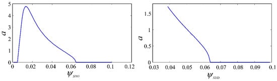
Figure 18.
The variation of the amplitude a with the dimensionless cutting depth (Ω = 1.2, , ρ = 11).
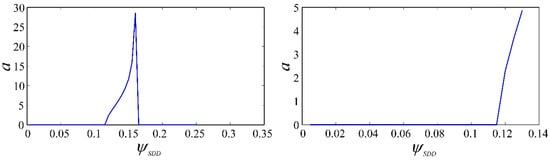
Figure 19.
The variation of the amplitude a with the dimensionless cutting depth (Ω = 2, , ρ = 11).
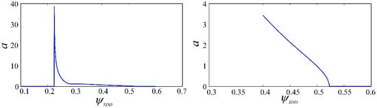
Figure 20.
The variation of the amplitude a with the dimensionless cutting depth (Ω = 4, , ρ = 11).
The results of the Hopf bifurcation of the CD model and the SDD model are compared. When Ω = 1.2 and 4, the Hopf bifurcation characteristic of SDD model is different from the subcritical Hopf bifurcation of the CD model; it is a kind of supercritical Hopf bifurcation. However, when Ω = 2, CD and SDD model are all subcritical Hopf bifurcation. The results show that the SDD model has some regions in supercritical Hopf bifurcation compared with the CD model.
On the other hand, the control parameter ρ increases from 11 to 30 when Ω = 4; the resulting amplitude curve is shown in Figure 21. In a supercritical Hopf state, the model is transformed from subcritical Hopf bifurcation at ρ = 11 to supercritical Hopf bifurcation at ρ = 30; the results of Figure 19b have thereby been proved. So we can change the Hopf bifurcation property of the drilling system by controlling the parameter ρ.
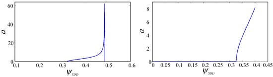
Figure 21.
The variation of the amplitude a with the dimensionless cutting depth (Ω = 4, , ρ = 30).
6. Conclusions
In order to control and avoid the stick-slip vibration in deep hole drilling, this paper simplified the drilling system to a two-degree-of-freedom discrete model and studied the non-linear dynamic stability without considering the bit bounce. There are two kinds of delay models (CD model and SDD model) in stick-slip vibration that are caused by regenerative cutting. The linear stability solved by the characteristic equations and Hopf bifurcation characteristics solved by the MMS are compared with the two delay models; our conclusions are as follows:
- The stability interval of the drilling system increases with rotational speed. In the linear stability analysis, the stability difference between CD model and SDD model is very small when the control parameter ρ is small. However, when the control parameter ρ become large, the stable intervals of the SDD model are bigger than those of the CD model, which means the SDD model can be applied to a wider operational range.
- It is found that there are only subcritical Hopf bifurcation regions in the CD model through the study of Hopf bifurcation properties. The Hopf bifurcation properties of the SDD model depend on the control parameter ρ. The subcritical Hopf bifurcation point on the right of the stability lobe is transformed into the supercritical Hopf bifurcation point with the increase of ρ.
- In the subcritical Hopf bifurcation point, the stable cutting points that co-exist with the limit cycle (stable periodic motion) in the system stability interval may also generate the stick-slip vibration. In the supercritical Hopf bifurcation point, the stable periodic motion co-exists with the cutting points of the linear unstable region, while the linear stable region does not have stable periodic motion. Therefore, the system will not produce stick-slip vibration in the stability interval.
In conclusion, the SDD model can be applied to a wider operational range than the CD model, and can better reflect the non-linear nature of the drilling system. On the one hand, the stability bounds of the SDD model are higher than for the CD model. On the other hand, the supercritical Hopf bifurcation point of the SDD model is more conductive to the stability of the drilling system. The method and results can be adopted for deep hole drilling stability prediction and provide a reference for the dynamic optimization design.
Author Contributions
J.H. and A.Z. conceived and designed the study; H.S. and S.S. performed the simulation; A.Z. and H.L. wrote the manuscript. H.L. and B.W. reviewed and edited the manuscript. All authors read and approved the manuscript.
Acknowledgments
This work was supported by the National Natural Science Foundation of China (Grant No. 51675091), the Joint Funds of the National Natural Science Foundation of China (Grant No. U1708257), and the Collaborative Innovation Center of Major Machine Manufacturing in Liaoning.
Conflicts of Interest
The authors declare no conflict of interest.
Appendix A
Appendix B
Appendix B.1. , , , and First- and Second-Order Forcing Functions and
Appendix B.2.
Substitution of Equations (50) and (51) into Equation (48) yields:
where
The particular solution of Equation (A18) can be obtained in the form:
where
Appendix B.3. Coefficient Vector , , , in Equation (53)
Appendix B.4. in Equation (54)
Taking the forcing vector associated with the secular components including (Equation (53)) gives:
Introducing a possible unstable solution vector of the form
into Equation (A35) and making the solution vector indeterminate, one obtains the solvability condition:
Rewriting Equation (A37) gives the modulation equation in complex form:
where
By comparing Equation (A39) with Equation (54), can be obtained as follows:
Appendix B.5. ,
References
- Richard, J.P. Time-delay Systems: An Overview of Some Recent Advances and Open Problems. Automatica 2013, 39, 1667–1694. [Google Scholar] [CrossRef]
- Kane, D.M.; Shore, K.A. Unlocking Dynamical Diversity: Optical Feedback Effects on Semiconductor Lasers; John Wiley & Sons: Hoboken, NJ, USA, 2005. [Google Scholar]
- Breakspear, M.; Roberts, J.A.; Terry, J.R. A Unifying Explanation of Primary Generalized Seizures through Nonlinear Brain Modeling and Bifurcation Analysis. Cereb. Cortex 2006, 16, 1296–1313. [Google Scholar] [CrossRef] [PubMed]
- Tobias, S.A. Machine-Tool Vibration; John Wiley & Sons: Hoboken, NJ, USA, 1965. [Google Scholar]
- Zamudio, C.A.; Tlusty, J.L.; Dareing, D.W. Self-Excited vibrations in Drillstrings. In Proceedings of the SPE Annual Technical Conference and Exhibition, Dallas, TX, USA, 27–30 September 1987; Society of Petroleum Engineers: Richardson, TX, USA, 1987. [Google Scholar]
- Leine, R.I.; Campen, D.H.; Kraker, A. Stick-Slip Vibrations Induced by Alternate Friction Models. Nonlinear Dyn. 1998, 16, 41–54. [Google Scholar] [CrossRef]
- Campen, D.H.; Keultjes, W.J.G. Stick-Slip Whirl Interaction in Drill String Dynamics. J. Vib. Acoust. 2002, 124, 209–220. [Google Scholar]
- Liao, C.M.; Balachandran, B.; Karkoub, M. Drill-String Dynamics: Reduced-Order Models and Experimental Studies. J. Vib. Acoust. 2011, 133, 041008. [Google Scholar] [CrossRef]
- Liao, C.M.; Vlajic, N.; Karki, H. Parametric Studies on Drill-String Motions. Int. J. Mech. Sci. 2012, 54, 260–268. [Google Scholar] [CrossRef]
- Vlajic, N.; Liao, C.M.; Karki, H. Draft: Stick-Slip Motions of a Rotor-Stator System. J. Vib. Acoust. 2014, 136, 021005. [Google Scholar] [CrossRef]
- Germay, C.; Sepulchre, R. Axial Stick-Slip Limit Cycling in Drill-String Dynamics with Delay. In Proceedings of the Fifth EUROMECH Nonlinear Dynamics Conference (ENOC), Indhoven, The Netherlands, 7–12 August 2005; pp. 1136–1143. [Google Scholar]
- Besselink, B.; Nijmeijer, H. A Semi-Analytical Study of Stick-Slip Oscillations in Drilling Systems. J. Comput. Nonlinear Dyn. 2011, 6, 021006. [Google Scholar] [CrossRef]
- Brett, J.F. The Genesis of Bit-Induced Torsional Drill String Vibrations. SPE Drill. Eng. 1992, 7, 168–174. [Google Scholar] [CrossRef]
- Fear, M.J.; Abbassian, F.; Parfitt, S.H.L. The Destruction of PDC Bits by Severe Slip-Stick Vibration. In Proceedings of the SPE/IADC Drilling Conference, Amsterdam, The Netherlands, 4–6 March 1997; Society of Petroleum Engineers: Richardson, TX, USA, 1997. [Google Scholar]
- Brett, J.F.; Warren, T.M.; Behr, S.M. Bit Whirl: A New Theory of PDC Bit Failure. In Proceedings of the SPE Annual Technical Conference and Exhibition, San Antonio, TX, USA, 8–11 October 1989; Society of Petroleum Engineers: Richardson, TX, USA, 1989. [Google Scholar]
- Warren, T.M.; Brett, J.F.; Sinor, L.A. Development of a Whirl-Resistant Bit. SPE Drill. Eng. 1990, 5, 267–275. [Google Scholar] [CrossRef]
- Richard, T.; Germay, C.; Detournay, E. A Simplified Model to Explore the Root Cause of Stick–Slip Vibrations in Drilling Systems with Drag Bits. J. Sound Vib. 2007, 305, 432–456. [Google Scholar] [CrossRef]
- Kovalyshen, Y. Understanding Root Cause of Stick–Slip Vibrations in Deep Drilling With Drag Bits. Int. J. Non-Linear Mech. 2014, 67, 331–341. [Google Scholar] [CrossRef]
- Stépán, G.; Kalmár, T. Nonlinear Regenerative Machine Tool Vibrations. In Proceedings of the 1997 ASME Design Engineering Technical Conferences, Sacramento, CA, USA, 14–17 September 1997. [Google Scholar]
- Wahi, P.; Chatterjee, A. Regenerative Tool Chatter Near a Codimension 2 Hopf Point Using Multiple Scales. Nonlinear Dyn. 2005, 40, 323–338. [Google Scholar] [CrossRef]
- Deshpande, N.; Fofana, M.S. Nonlinear Regenerative Chatter in Turning. Robot. Comput. Integr. Manuf. 2001, 17, 107–112. [Google Scholar] [CrossRef]
- Stépán, G.; Insperger, T.; Szalai, R. Delay, Parametric Excitation, and the Nonlinear Dynamics of Cutting Processes. Int. J. Bifurc. Chaos 2005, 15, 2783–2798. [Google Scholar] [CrossRef]
- Hanna, N.H.; Tobias, S.A. A Theory of Nonlinear Regenerative Chatter. ASME J. Eng. Ind. 1974, 96, 247–255. [Google Scholar] [CrossRef]
- Shi, H.M.; Tobias, S.A. Theory of Finite Amplitude Machine Tool Instability. Int. J. Mach. Tool Des. Res. 1984, 24, 45–69. [Google Scholar] [CrossRef]
- Insperger, T.; Stépán, G.; Turi, J. State-Dependent Delay in Regenerative Turning Processes. Nonlinear Dyn. 2007, 47, 275–283. [Google Scholar] [CrossRef]
- Insperger, T.; Barton, D.A.W.; Stépán, G. Criticality of Hopf Bifurcation in State-Dependent Delay Model of Turning Processes. Int. J. Non-Linear Mech. 2008, 43, 140–149. [Google Scholar] [CrossRef]
- Long, X.H.; Balachandran, B. Milling Model with Variable Time Delay. In Proceedings of the ASME 2004 International Mechanical Engineering Congress and Exposition, Anaheim, CA, USA, 13–19 November 2004; pp. 933–940. [Google Scholar]
- Long, X.H.; Balachandran, B.; Mann, B.P. Dynamics of Milling Processes with Variable Time Delays. Nonlinear Dyn. 2007, 47, 49–63. [Google Scholar] [CrossRef]
- Richard, T.; Germay, C.; Detournay, E. Self-Excited Stick–Slip Oscillations of Drill Bits. C. R. Mec. 2004, 332, 619–626. [Google Scholar] [CrossRef]
- Richard, T.; Detournay, E.; Fear, M. Influence of Bit-Rock Interaction on Stick-Slip Vibrations of PDC Bits. In Proceedings of the SPE Annual Technical Conference and Exhibition, San Antonio, TX, USA, 29 September–2 October 2002. [Google Scholar]
- Stepan, G. Retarded Dynamical Systems; Longman: Harlow, UK, 1989. [Google Scholar]
- Altintaş, Y.; Budak, E. Analytical Prediction of Stability Lobes in Milling. CIRP Ann. Manuf. Technol. 1995, 44, 357–362. [Google Scholar] [CrossRef]
- Balachandran, B.; Zhao, M.X. A Mechanics Based Model for Study of Dynamics of Milling Operations. Meccanica 2000, 35, 89–109. [Google Scholar] [CrossRef]
- Insperger, T.; Mann, B.P.; Stépán, G. Stability of Up-Milling and Down-Milling, Part 1: Alternative Analytical Methods. Int. J. Mach. Tools Manuf. 2003, 43, 25–34. [Google Scholar] [CrossRef]
- Merdol, S.D.; Altintas, Y. Multi Frequency Solution of Chatter Stability for Low Immersion Milling. J. Manuf. Sci. Eng. 2004, 126, 459–466. [Google Scholar] [CrossRef]
- Liu, X.; Vlajic, N.; Long, X. Coupled Axial-Torsional Dynamics in Rotary Drilling With State-Dependent Delay: Stability and Control. Nonlinear Dyn. 2014, 78, 1891–1906. [Google Scholar] [CrossRef]
- Liu, X.; Vlajic, N.; Long, X. State-Dependent Delay Influenced Drill-String Oscillations and Stability Analysis. J. Vib. Acoust. 2014, 136, 051008. [Google Scholar] [CrossRef]
- Nandakumar, K.; Wiercigroch, M. Stability Analysis of a State Dependent Delayed, Coupled Two DOF Model of Drill-String Vibration. J. Sound Vib. 2013, 332, 2575–2592. [Google Scholar] [CrossRef]
- Insperger, T.; Stépán, G.; Hartung, F. State Dependent Regenerative Delay in Milling Processes. In Proceedings of the ASME 2005 International Design Engineering Technical Conferences and Computers and Information in Engineering Conference, Long Beach, CA, USA, 24–28 September 2005; pp. 955–964. [Google Scholar]
- Hartung, F.; Turi, J. On Differentiability of Solutions With Respect to Parameters in State-Dependent Delay Equations. J. Differ. Equ. 1997, 135, 192–237. [Google Scholar] [CrossRef]
- Kim, P.; Seok, J. Bifurcation analyses on the chatter vibrations of a turning process with state-dependent delay. Nonlinear Dyn. 2012, 69, 891–912. [Google Scholar] [CrossRef]
© 2018 by the authors. Licensee MDPI, Basel, Switzerland. This article is an open access article distributed under the terms and conditions of the Creative Commons Attribution (CC BY) license (http://creativecommons.org/licenses/by/4.0/).