A Novel Hybrid Approach to Deal with DVL Malfunctions for Underwater Integrated Navigation Systems

Abstract

As a common device for underwater integrated navigation systems, Doppler velocity log (DVL) has the risk of malfunction. To improve the reliability of navigation systems, a hybrid approach is presented to forecast the measurements of the DVL while it malfunctions. The approach employs partial least squares regression (PLSR) coupled with support vector regression (SVR) to build a hybrid predictor. As the current and past calculating velocities of strapdown inertial navigation system (SINS) are taken as the predictor’s inputs, PLSR is applied to cope with the situation where there exists intense relativity among independent variables. Since PLSR is a linear regression, SVR is used to predict the residual components of the PLSR prediction to improve the accuracy. When the DVL works well, the hybrid predictor is trained online as a backup, whereas during malfunctions, the predictor offers the estimation of the DVL measurements for information fusion. The performance of the proposed approach is verified with simulations based on SINS/DVL/MCP/pressure sensor (PS) integrated navigation system. The comparison results indicate that the PLSR-SVR hybrid predictor can correctly provide the estimated DVL measurements and effectively extend the tolerance time on DVL malfunctions, thereby improving the navigation accuracy and reliability.

1. Introduction

With the increasing development of ocean exploration, underwater vehicles, including remotely operated vehicles (ROVs) and autonomous underwater vehicles (AUVs), are employed to perform underwater tasks, such as bathymetric data collection and marine mining exploration [1,2]. To successfully complete the scheduled tasks, an accurate and reliable navigation system is indispensable for underwater vehicles.

Due to the advantages of high reliability and complete independence, the strapdown inertial navigation system (SINS) is commonly used for underwater navigation. The SINS provides velocity, position and attitude of the vehicle using the information obtained by the inertial measurement unit (IMU). The IMU is composed of gyroscopes and accelerometers to measure the angular rates and the specific forces respectively. The navigation errors of the SINS increase with time due to the inherent bias errors of gyroscopes and accelerometers [3,4,5]. Therefore, in order to improve the navigation performance, it is necessary to introduce auxiliary sensors to limit the error growth of the SINS. Now the integrated navigation system which consists of multiple navigation sensors is widely adopted on underwater vehicles [6,7,8]. As a high-precision velocity measuring instrument, the Doppler velocity log (DVL) has become increasingly popular as the fundamental component of underwater integrated navigation systems [9,10,11,12,13].

The DVL provides the velocities relative to the seafloor or the current based on the Doppler effect [14]. By using a Kalman filter (KF), the highly accurate velocities provided by the DVL can be used to effectively restrain the error accumulation of the SINS [15,16]. However, the dependency of the DVL signal on the acoustic environment may occasionally make the DVL malfunction [4]. Taking into account the work-mode against the seafloor in various seafloor environments, the DVL may malfunction in the following circumstances (shown in Figure 1):

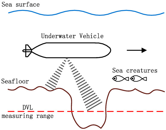
Figure 1. DVL malfunction circumstances.

(1)

When the underwater vehicle sails across sea creatures, the acoustic wave emitted by the DVL cannot reach the seafloor.

(2)

When the strong wave-absorbing material (such as sludge) exists in the seafloor, the acoustic wave emitted by the DVL cannot be reflected back.

(3)

When the underwater vehicle sails over a trench, the distance between the vehicle and the bottom of the trench exceeds the measuring range of the DVL.

(4)

When the underwater vehicle performs large angle maneuvers, the DVL could malfunction under the condition of large roll and pitch.

If the above-mentioned situations occur, it could lead to the loss of the DVL signal or the sudden changes of the velocity obtained from the DVL, and consequently the KF cannot get reliable external velocity information, which will cause the SINS errors to accumulate. As a result, the navigation system of the underwater vehicle cannot provide accurate navigation information anymore. So how to deal with DVL malfunctions for underwater integrated navigation systems is crucial. Over the past few decades, many solutions have been proposed to deal with sensor malfunctions in integrated navigation systems. The existing approaches can be classified into two broad categories: one is masking the faulty sensor or isolating the malfunction, and the other is finding a replacement for the faulty sensor or the KF.

The first category is mostly implemented by two approaches: the use of hardware redundancy [17,18], and the adjustment of navigation sensors utilization [19,20,21]. Mirabadi et al. [17] proposed a navigation system with two INS systems. By designing the hierarchical structure of the filters, each branch includes one of the INS sensors. Once one of INS sensors malfunctions, the system will shift to the other branch with the non-faulty INS sensor. This approach can deal with the malfunction for a long time but requires high hardware cost. To restrain the cost, approaches are developed based on filter technique to tune the utilization of sensor measurements. Ushaq and Fang [19] introduced the weighting factors to adjust the contribution of each local filter in the final data fusion for the SINS/GPS/CNS system. The weighting factor which is computed using fuzzy inference system will be close to zero in a failure. Li and Zhang [20] introduced the degree of confidence which indicates the level at which the local filter information fusion is dependent on its filter information after the measurement update. In the event of malfunction, the degree of confidence will be quite low, and accordingly, the influence of the filter information after measurement update will be very little. This kind of approaches is cost saving, but there is the potential risk of cross contamination. There are also other researchers working to find a replacement for the KF [22,23,24,25], and various models have been built to predict the errors of the reference system. Semeniuk and Noureldin [23] proposed an artificial-intelligence-based segmented forward predictor to overcome situations of GPS satellite signals blockage. By employing radial basis function neural networks, the predictor provides the INS position and velocity errors. Hasan et al. [24] introduced a genetic neuro-fuzzy system to predict the INS errors during the GPS failures. These intelligent algorithms can solve sensor failures without requiring any prior information about the characteristics of the sensors. In addition, this kind of method is attracting more and more attention.

In this paper, a hybrid approach based on partial least squares regression (PLSR) and support vector regression (SVR) is proposed to deal with short-term DVL malfunctions for underwater integrated navigation systems. We aim to build a predictor which can estimate the measurements of the DVL when it malfunctions. The predictor is devoted to establish the relationship between the SINS outputs and the DVL outputs, taking into consideration the changing trend of the velocity, current and past calculating velocities of the SINS as the predictor’s inputs. In order to improve the predictor robustness in the presence of intense relativity among independent variables, PLSR is employed to simulate the velocity measurements of the DVL. Considering that the PLSR model is linear, SVR is used to estimate the residual components of the PLSR prediction to improve the accuracy. When the DVL works well, the PLSR-SVR predictor is trained using the SINS calculating velocities as the inputs and the actual DVL velocity measurements as the outputs. When the DVL malfunctions, the invalid measurements of the DVL will be temporarily substituted by the prediction outputs of PLSR-SVR predictor. To confirm the validity of the proposed approach, comparative simulations and field tests are carried out. The results demonstrate that the PLSR-SVR hybrid predictor can correctly provide the estimated measurements for DVL and effectively extend the tolerance time on DVL malfunctions, which can greatly improve the accuracy and reliability of the underwater integrated navigation system. The contributions of this paper are briefly listed as follows. (1) In existing results, faulty sensors of integrated navigation systems have been popularly addressed. The most popular method which attempts to replace KF is based on connecting the SINS error to the corresponding SINS output. However, this would affect the accuracy of the navigation system. This paper does not aim to find a replacement for the KF, but to develop a measurement predictor for the faulty sensor to aid the KF. (2) The existing methods concentrate mostly on the dependence of the prediction on the SINS output at certain time instants, but the dependence on the past outputs of the SINS has not been taken into account. In this study, both the current and the past outputs of the SINS are taken as the inputs of the predictor to improve the accuracy of prediction.

The rest of the paper is organized into the following sections: Section 2 describes the underwater integrated navigation system of SINS/DVL/MCP/PS; Section 3 presents the PLSR-SVR hybrid predictor and its implementation in the integrated navigation system; Section 4 provides simulations and field tests along with specific analysis; Section 5 is committed to concluding remarks.

2. Underwater Integrated Navigation System

2.1. System Structure

As mentioned in the previous section, auxiliary sensors are necessary to assist the SINS for high accuracy. In an underwater integrated navigation system, commonly used aiding equipment include DVL, magnetic compass (MCP), pressure sensor (PS), global positioning system (GPS), acoustic positioning system (APS) and geophysical navigation system (GNS, such as terrain aided navigation and gravity aided navigation). Unfortunately, the GPS signals are unavailable under water, so the vehicle with GPS needs to surface regularly. APS requires the vehicle to be placed within the coverage area of transponders, which limits the operation range of the vehicle. Similarly, GNS restricts the vehicle to work in the area where certain geography information is known. The DVL, without the need to use external sources, is a popular sensor to assist the SINS in underwater environment. Unfortunately, the observability of heading is low for SINS/DVL integrated navigation system, therefore a MCP is adopted to provide heading information. In addition, a PS is used to provide height (or depth) information due to the divergence of the height from the SINS and the low accuracy of the vertical velocity from the DVL [4,22]. Accordingly, SINS/DVL/MCP/PS integrated navigation system is established to perform independent underwater navigation.

Figure 2 shows the system structure of the SINS/DVL/MCP/PS integrated navigation system. Because of its less computational effort and high fault-tolerance, the federated filter is adopted to fuse the multi-sensor data. The SINS is the reference system providing continuous velocity, attitude and position information. Three local filters implemented with KF are composed of the DVL, the MCP and the PS assisting the SINS, respectively. The measurement deviation between the SINS and the assistant navigation observer is given to the corresponding local filter as input. Since the DVL provides the velocity measurements in the body frame (b frame), the outputs of the DVL need to be transformed to the navigation frame (n frame) by the attitude matrix obtained from the SINS.

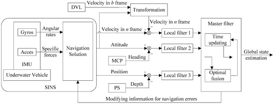
Figure 2. System structure based on the federated filter.

2.2. System Model

Set the Right-Front-Up (RFU) frame as the body frame, and the East-North-Up (ENU) geographic coordinates as the navigation frame. The error state vector of the integrated navigation system is set as

$$X_k={[{\varphi }_e{\varphi }_n{\varphi }_u\delta V_e\delta V_n\delta V_u\delta L\delta \lambda \delta h{\epsilon }_x{\epsilon }_y{\epsilon }_z{\nabla }_x{\nabla }_y{\nabla }_z]}^T$$

(1)

where φ_e φ_n φ_u are attitude errors. δV_e, δV_n, δV_u are velocity errors. δL, δλ, δh are position errors. ε_x, ε_y, ε_z are gyroscope drifts. ${\nabla }_x$, ${\nabla }_y$, ${\nabla }_z$ are accelerometer biases.

The system equation and the measurement equation for the local filters can be expressed as follows.

$$\{\begin{array}{l}{X}_k={\Phi }_{k,k-1}{X}_{k-1}+W_k\hfill \\ Z_k=H_k{X}_k+V_k\hfill \end{array}$$

(2)

where X_k−1 is the error states of the integrated navigation system at time t_k−1, and X_k is the error states at time t_k. Φ_k,k−1 is the state transition matrix from time t_k−1 to t_k. Z_k is the measurement vector. H_k is the measurement matrix. W_k and V_k are assumed to be a zero mean white noise sequence with known covariance Q_k and R_k, respectively.

The integration of the DVL and the SINS is processed in the local filter 1. The measurement model of the local filter 1 can be constructed as

$$\begin{array}{ll}{Z}_k^{(1)}& ={\left(\begin{array}{ccc}{V}_{eSINS}^n-V_{eDVL}^n& V_{nSINS}^n-V_{nDVL}^n& V_{uSINS}^n-V_{uDVL}^n\end{array}\right)}^T\hfill \\ & =H_k^{(1)}{X}_k^{(1)}+V_k^{(1)}\hfill \end{array}$$

(3)

where the superscript n denotes the navigation frame. As mentioned, the DVL provides the velocity measurements in the body frame and hence could not be used as the measurement for alignment directly. $V_{eDVL}^n$, $V_{nDVL}^n$ and $V_{uDVL}^n$ are the projected velocity of the DVL measurements in the navigation frame, which can be calculated according to the following formula.

$$V_{DVL}^n=C_b^n{V}_{DVL}^b$$

(4)

where $V_{DVL}^b$ is the DVL velocity measurements in the body frame. $C_b^n$ is the transformation matrix from the body frame to the navigation frame, which can be expressed with the attitude angles.

According to the relationship between the measurement vector and the error state vector, the measurement matrix of the local filter 1 can be expressed as follows.

$$H_k^{(1)}=\left(\begin{array}{ccc}{0}_{3\times 3}& I_{3\times 3}& 0_{3\times 9}\end{array}\right)$$

(5)

where I_3×3 is a 3 × 3 identity matrix. 0_m×n is a zero matrix with m rows and n columns.

The covariance matrix of the DVL measurements caused by instrumental noise is given in [26], namely.

$$R_k^{(1)}=\left(\begin{array}{ccc}\frac{{\sigma }_{b_1}^2+{\sigma }_{b_2}^2}{4{\sin }^2\beta }& 0& \frac{{\sigma }_{b_1}^2-{\sigma }_{b_2}^2}{8\sin \beta \cos \beta }\\ 0& \frac{{\sigma }_{b_3}^2+{\sigma }_{b_4}^2}{4{\sin }^2\beta }& \frac{{\sigma }_{b_4}^2-{\sigma }_{b_3}^2}{8\sin \beta \cos \beta }\\ \frac{{\sigma }_{b_1}^2-{\sigma }_{b_2}^2}{8\sin \beta \cos \beta }& \frac{{\sigma }_{b_4}^2-{\sigma }_{b_3}^2}{8\sin \beta \cos \beta }& \frac{{\sigma }_{b_1}^2+{\sigma }_{b_2}^2+{\sigma }_{b_3}^2+{\sigma }_{b_4}^2}{16{\cos }^2\beta }\end{array}\right)$$

(6)

where ${\sigma }_{b_i}^2$ is the variance of the radial velocity due to instrumental noise along the beam i (i = 1, 2, 3, 4). Assume that the radial velocity variances are equal, and then the covariance matrix can be simplified as

$$R_k^{(1)}=\left(\begin{array}{ccc}{\sigma }_{v_x}^2& 0& 0\\ 0& {\sigma }_{v_y}^2& 0\\ 0& 0& {\sigma }_{v_z}^2\end{array}\right)$$

(7)

where the diagonal elements are the variance of the DVL measurement along the body frame.

The local filter 2 is responsible for fusing the MCP and the SINS. In parallel, the local filter 3 is in charge of the fusion between the PS and the SINS. The measurement models of these two filters can be constructed respectively as

$$Z_k^{(2)}=\left(H_{SINS}-H_{MCP}\right)=H_k^{(2)}{X}_k^{(2)}+V_k^{(2)}$$

(8)

$$Z_k^{(3)}=\left(h_{SINS}-h_{PS}\right)=H_k^{(3)}{X}_k^{(3)}+V_k^{(3)}$$

(9)

where H_SINS and H_MCP denote the heading provided by the SINS and the MCP, respectively. h_SINS and h_PS denote the height offered by the SINS and the PS, respectively. The measurement matrixes can be described as

$$H_k^{(2)}=\left(\begin{array}{ccc}{0}_{1\times 2}& 1& 0_{1\times 12}\end{array}\right)$$

(10)

$$H_k^{(3)}=\left(\begin{array}{ccc}{0}_{1\times 8}& 1& 0_{1\times 6}\end{array}\right)$$

(11)

The measurement noise variances of the MCP and the PS are defined respectively by

$$R_k^{(2)}={\sigma }_H^2$$

(12)

$$R_k^{(3)}={\sigma }_h^2$$

(13)

where ${\sigma }_H^2$ and ${\sigma }_h^2$ are the variance of the MCP measurement and the PS measurement, respectively.

The master filter is in charge of fusing the local state estimates. If all subsystems are independent, the fusion algorithm can be presented as follows.

$$P_k^g={[{(P_k^{(1)})}^{-1}+{(P_k^{(2)})}^{-1}+{(P_k^{(3)})}^{-1}]}^{-1}$$

(14)

$${\widehat{X}}_k^g=P_k^g\cdot [{(P_k^{(1)})}^{-1}\cdot {\widehat{X}}_k^{(1)}+{(P_k^{(2)})}^{-1}\cdot {\widehat{X}}_k^{(2)}+{(P_k^{(3)})}^{-1}\cdot {\widehat{X}}_k^{(3)}]$$

(15)

where ${\widehat{X}}_k^g$ denotes the global state estimation. ${\widehat{X}}_k^{(1)}$, ${\widehat{X}}_k^{(2)}$ and ${\widehat{X}}_k^{(3)}$ are the estimates of the error states obtained from the local filters. $P_k^{(1)}$, $P_k^{(2)}$ and $P_k^{(3)}$ are the covariance matrixes of ${\widehat{X}}_k^{(1)}$, ${\widehat{X}}_k^{(2)}$ and ${\widehat{X}}_k^{(3)}$, respectively. $P_k^g$ is the covariance matrix of ${\widehat{X}}_k^g$. The DVL, MCP and PS are run independent, which satisfies the requirement of the formulas.

3. Proposed PLSR-SVR Hybrid Predictor

It is obvious that there is a connection between the SINS outputs and the DVL outputs. Moreover, the SINS is more reliable, so we aim to establish the relationship between the SINS calculating results and the DVL measurements. Thus, the measurements of the DVL can be predicted when it malfunctions. It is worth mentioning that the employed SINS calculating results are revised by the closed-loop KF. In order to improve the prediction accuracy and reliability, both the current and the past calculating velocities of the SINS are taken as the inputs of the predictor. In this case, strong relevance exists between the independent variables, which could possibly compromise the robustness of the predictor. To solve the problem, partial least squares regression (PLSR) which is good at dealing with multi-collinearity, is employed to build the predictor. Since PLSR is a kind of linear regression, a nonlinear regression model is necessary to further improve the prediction precision. Here, support vector regression (SVR) is chosen to overcome the shortcomings of PLSR. The hybrid approach of linear and nonlinear regression models has proven to be effective [27,28]. The proposed hybrid approach combines the advantages of both PLSR and SVR, thus effectively handling the complex data relationship (including linear and nonlinear relationships). The specific implementation of the hybrid predictor is presented below.

3.1. PLSR for the Prediction of the DVL Measurements

PLSR was first proposed by Wold et al. in 1983 [29]. As a multivariate statistical analysis method, PLSR is mainly used for modeling between multi-independent variables and multi-dependent variables. By decomposing and selecting the data information, PLSR identifies useful information and noise to overcome the problems caused by the intense relativity between independent variables. The algorithm of PLSR is introduced below.

There are p independent variables (x₁, …, x_p) and q dependent variables (y₁, …, y_q). By observing l sample points, a data matrix of independent variable X = [x₁, …, x_p]_l×p and a data matrix of dependent variable Y = [y₁, …, y_q]_l×q are obtained. The aim of PLSR is to form the structure between X and Y, and to predict Y via X [30]. The first latent vector t₁ and u₁ are extracted from X and Y respectively, and the principles of the extraction are shown as follows.

(1)

t₁ and u₁ should carry as much the diversity information of the corresponding data matrix as possible.

(2)

The degree of correlation between t₁ and u₁ should reach its maximum.

Once the above principles are satisfied, X and Y will be well represented by t₁ and u₁ respectively. Besides, t₁ would have the strongest interpretation for u₁. Then X and Y can be expressed with t₁. If the regression achieves satisfactory precision, the algorithm ends. Otherwise, the second latent vector needs to be extracted from the residual matrix. Repeat the process until an acceptable accuracy is obtained. Suppose m latent vectors (that is, t₁, …, t_m) have been extracted, the dependent variables y_k (k = 1, 2, …, q) can be expressed with t₁, …, t_m. By the transition, y_k (k = 1, 2, …, q) can be expressed with x₁, …, x_p in the end.

The above algorithm is formalized as follows.

Step 1: The data matrices X and Y are standardized (mean-centered and scaled to unite variances) as

$$E_0={\left(E_{01},\dots ,E_{0p}\right)}_{l\times p},F_0={\left(F_{01},\dots ,F_{0q}\right)}_{l\times q}$$

(16)

Step 2: Calculate the weight vector w₁ which is the eigenvector corresponding to the greatest eigenvalue of the matrix $E_0{}^T{F}_0{F}_0{}^T{E}_0$.

Step 3: Calculate the latent vector t₁.

$$t_1=E_0{w}_1$$

(17)

Step 4: Calculate the loading vectors p₁ and r₁.

$$p_1=\frac{E_0{}^T{t}_1}{{\Vert t_1\Vert }^2},r_1=\frac{F_0{}^T{t}_1}{{\Vert t_1\Vert }^2}$$

(18)

Step 5: Calculate the residual matrices E₁ and F₁.

$$E_1=E_0-t_1{p}_1{}^T,F_1=F_0-t_1{r}_1{}^T$$

(19)

Step 6: If the stopping criterion is met, end the iteration. Otherwise, replace E₀ and F₀ with E₁ and F₁, and go to Step 2.

Suppose the iteration stops at the hth iteration, and h latent vectors (that is, t₁, …, t_h) are obtained. F₀ can then be expressed with the latent vectors as

$$F_0=t_1{r}_1{}^T+\cdots +t_h{r}_h{}^T+F_h$$

(20)

where F_h is the residual matrix of F₀ when the h latent vectors are included in the PLSR method.

By using Equations (17) and (20), an expression for F₀ in terms of E₀ can be derived by means of the mathematical induction.

$$F_0=E_0\left\{w_1{r}_1{}^T+{\displaystyle \sum _{i=2}^h\left({\displaystyle \prod _{j=1}^{i-1}\left(I-w_j{p}_j{}^T\right)}\right)w_i{r}_i{}^T}\right\}+F_h$$

(21)

Finally, the regression equation of Y about X with regard to the PLSR model can be obtained according to Equation (21).

When the DVL is working properly, the training samples for PLSR contain the SINS calculating results (specifically, velocities along the navigation frame) as inputs and the DVL measurements as desired outputs. To improve the prediction accuracy and reliability, both the current and the past calculating velocities of the SINS are used as the inputs for PLSR. Assume the DVL works well during time T−s to time T, the data matrix of independent variable X and the data matrix of dependent variable Y are represented respectively as

$$X={\left[V_{eSINS(T-s)}^n,V_{nSINS(T-s)}^n,V_{uSINS(T-s)}^n,\dots ,V_{eSINS(T)}^n,V_{nSINS(T)}^n,V_{uSINS(T)}^n\right]}_{l\times (3s+3)}$$

(22)

$$Y={\left[V_{eDVL(T)}^n,V_{nDVL(T)}^n,V_{uDVL(T)}^n\right]}_{l\times 3}$$

(23)

where l is the training sample size for PLSR. The PLSR predictor is trained with the above data matrices. As previously stated, the aim of training is to get the linear regression model of X and Y by extracting the latent vectors (t₁, …, t_h). Steps 1–6 describes the training process in detail. Then the PLSR prediction model can be obtained according to Equation (21). When the DVL fails, the PLSR predictor is working to predict the DVL measurements. Assume the DVL malfunctions at time T₀, the input for the PLSR predictor is correspondingly described as $\left(V_{eSINS(T_0-s)}^n,V_{nSINS(T_0-s)}^n,V_{uSINS(T_0-s)}^n,\dots ,V_{eSINS(T_0)}^n,V_{nSINS(T_0)}^n,V_{uSINS(T_0)}^n\right)$. Then the PLSR predictor outputs the prediction of the DVL measurements, symbolized by ${\widehat{V}}_{DVL\_P(T_0)}^n$. Figure 3 shows the flow chart of the above algorithm. The dashed box in Figure 3 indicates the training process of PLSR.

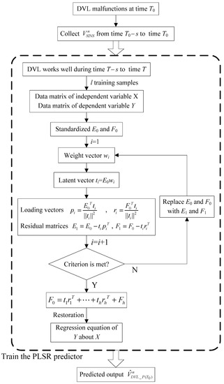
Figure 3. The prediction based on PLSR.

3.2. SVR for the Prediction of the Residual Components

Since PLSR is linear, the predictor can only handle the linear relationship between the independent variables and the dependent variables. In order to improve the prediction accuracy, SVR is introduced to predict the residual components of PLSR. SVR is based on extension of the support vector concept proposed by Vapnik et al. [31]. The aim of SVR is to provide a nonlinear mapping function to map the training data to a high dimension feature space [32]. The algorithm of SVR is introduced below.

There is a sample set S = {(x_i, y_i)}, where x_i and y_i are the input vector and the target output respectively. In the high dimension feature space, there theoretically exists a linear function f to formulate the nonlinear relationship between x_i and y_i [33]. The function is called the SVR function, which is defined as

$$f(x)=v^T\varphi (x)+b$$

(24)

where v is the weight vector. φ(x) is the mapping function to map x to a high dimension feature space. b is the bias term.

The training error of SVR is determined by the ε-insensitivity loss function which is defined as follows.

$${\left|y-f(x)\right|}_{\epsilon }=\{\begin{array}{c}0\\ \left|y-f(x)\right|-\epsilon \end{array}\begin{array}{c}\left|y-f(x)\right|\le \epsilon \\ \mathrm{otherwise}\end{array}$$

(25)

where ε is the insensitivity loss zone. The ε-insensitivity loss function can improve the robustness of the regression.

Different from the traditional regression models that estimate the coefficients through minimizing the loss square, SVR aims to minimize the empirical and structural risk. Then the regression problem is equivalent to the problem of minimizing the cost function which is described as

$$\min \frac{1}{2}{v}^{T}v+C{\displaystyle \sum _{i=1}^m({\xi }_i+{\xi }_i^{*})}$$

(26)

$$s.t.\{\begin{array}{l}{y}_i-v^T\varphi (x_i)-b\le \epsilon +{\xi }_i\hfill \\ v^T\varphi (x_i)+b-y_i\le \epsilon +{\xi }_i^{*}\hfill \\ {\xi }_i\ge 0,{\xi }_i^{*}\ge 0\hfill \end{array}$$

(27)

where m is the number of the training sample. $\frac{1}{2}{v}^{T}v$ is the structural risk to prevent overtraining error. ${\xi }_i$ and ${\xi }_i^{*}$ are the positive slack variables which are used to measure the deviation of insensitive boundaries. (${\xi }_i$ + ${\xi }_i^{*}$) is the empirical risk. C is a constant to balance between the empirical and structural risk.

By using the method of Lagrange multiplier and the Karush-Kuhn-Tucker condition, the dual problem of the Formula (27) can be described as

$$\max L(\alpha ,\alpha *)=-\frac{1}{2}{\displaystyle \sum _{i,j=1}^m({\alpha }_i-{\alpha }_i^{*})({\alpha }_j-{\alpha }_j^{*})}K(x_i,x_j)-\epsilon {\displaystyle \sum _{i=1}^m({\alpha }_i+{\alpha }_i^{*})}+{\displaystyle \sum _{i=1}^m{y}_i({\alpha }_i-{\alpha }_i^{*})}$$

(28)

$$s.t.{\displaystyle \sum _{i=1}^m({\alpha }_i-{\alpha }_i^{*})}=0(0\le {\alpha }_i,{\alpha }_i^{*}\le Ci=1,\dots ,m)$$

(29)

where α_i and ${\alpha }_i^{*}$ are the Lagrange multipliers. By solving the above equations, we can get the values of α_i and ${\alpha }_i^{*}$. Then v can be calculated by

$$v={\displaystyle \sum _{i=1}^m({\alpha }_i-{\alpha }_i^{*})\varphi (x_i)}$$

(30)

Finally, the SVR function can be obtained as

$$f(x)={\displaystyle \sum _{i=1}^m({\alpha }_i-{\alpha }_i^{*})K(x,x_i)}+b$$

(31)

where K(x, x_i) is the kernel function with the value of the inner product <φ(x), φ(x_i)>. Kernel functions, including polynomial kernel function, radial basic function and Sigmoid kernel function are often used. In this paper, the radial basic function is chosen to be the kernel function, which is expressed as

$$K(x,x_i)=\exp (-{\left|x-x_i\right|}^2/{\sigma }^2)$$

(32)

where σ is the width of the radial basis function.

When the DVL is working properly, the SINS calculating results are taken as the input for the PLSR predictor. The predictor outputs the prediction of the DVL measurements ${\widehat{V}}_{DVL\_P}^n$. The residual components of the PLSR prediction can be calculated by

$$\delta V_{DVL}^n=V_{DVL}^n-{\widehat{V}}_{DVL\_P}^n$$

(33)

where $V_{DVL}^n$ is the velocity measurements of the DVL. Assume the DVL works well at time T, the sample set for SVR contains the SINS calculating velocities (i.e., $\left(V_{eSINS(T)}^n,V_{nSINS(T)}^n,V_{uSINS(T)}^n\right)$) as inputs and the residual components of the PLSR prediction (i.e., $\delta V_{eDVL(T)}^n$, $\delta V_{nDVL(T)}^n$ and $\delta V_{uDVL(T)}^n$) as desired outputs. The SVR predictor is trained with the sample set. As stated above, there are two parameters to be determined in the training process, i.e., the Lagrange multipliers α_i and α*. The two parameters can be obtained by solving the problem listed in Equations (28) and (29). After obtaining the Lagrange multipliers, the SVR prediction model can be formed by Equation (31). When the DVL fails, the SVR predictor is employed to predict the residual of PLSR. Assume the DVL malfunctions at time T₀, the input for the SVR predictor is described as $\left(V_{eSINS(T_0)}^n,V_{nSINS(T_0)}^n,V_{uSINS(T_0)}^n\right)$. Then the SVR predictor outputs the prediction of the residual components, symbolized by $\delta {\widehat{V}}_{eDVL\_S(T_0)}^n$, $\delta {\widehat{V}}_{nDVL\_S(T_0)}^n$ and $\delta {\widehat{V}}_{uDVL\_S(T_0)}^n$.

3.3. PLSR-SVR Hybrid Predictor

When the DVL works well, its outputs can be used to provide the inputs for the KF by subtracting the SINS with DVL velocity measurements. At this time, the PLSR-SVR hybrid predictor works in the modeling mode. To train the PLSR predictor, the current and past calculating velocities of the SINS are used as the predictor inputs, and the DVL velocity measurements are treated as the training target. Besides, the prediction ${\widehat{V}}_{DVL\_P}^n$ by the PLSR predictor subtracted from the DVL measurement $V_{DVL}^n$ gives the residual component $\delta V_{DVL}^n$. The predictor of $\delta V_{DVL}^n$ is developed based on SVR. The training processes of PLSR and SVR are described in detail in Section 3.1 and Section 3.2 respectively. During this modeling process, the proposed PLSR-SVR hybrid model is adjusted online with the update of the SINS and DVL measurements. Figure 4 shows the block diagram of modeling mode when the DVL works well.

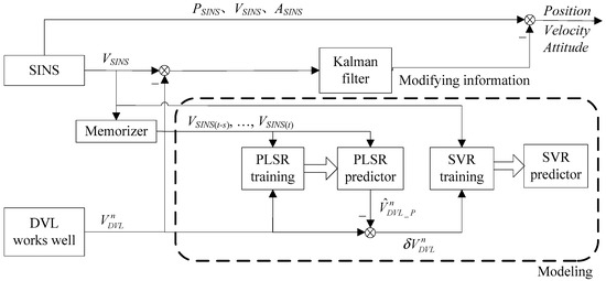
Figure 4. The block diagram of modeling mode.

When the DVL malfunctions, it can not provide valid measurements. At this time, the PLSR-SVR hybrid predictor switches to the prediction mode. The PLSR predictor uses the current and past calculating velocities of the SINS as inputs to generate the prediction ${\widehat{V}}_{DVL\_P}^n$. At the same time, the SVR predictor outputs the prediction $\delta {\widehat{V}}_{DVL\_S}^n$ by taking the SINS calculating velocities as inputs. The results of the two predictors are added to form an optimal prediction of the DVL measurement ${\widehat{V}}_{DVL}^n$. Finally, ${\widehat{V}}_{DVL}^n$ is used to substitute for the invalid measurements of the DVL during its malfunction. Figure 5 shows the block diagram of prediction mode when the DVL fails.

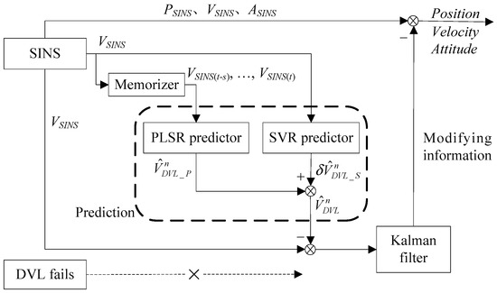
Figure 5. The block diagram of prediction mode.

4. Performance Evaluation

4.1. Simulations and Results

Simulations are carried out to validate the proposed approach. The PLSR-SVR hybrid predictor is employed to deal with DVL malfunctions for the SINS/DVL/MCP/PS integrated navigation system. The specifications of the instruments used are listed in Table 1. The time of simulation is 1500 s. Figure 6 shows the trajectory of the underwater vehicle. The initial latitude, longitude and height of the underwater vehicle are set as 32° N, 118° E and −20 m. The vehicle travels from point A to point B. The vehicle movements include acceleration, deceleration, turning, diving and surfacing. The detailed motion states of the vehicle are listed in Table 2. The proposed hybrid model is trained during the DVL normal operations and the trained model is further utilized for the predictions during the DVL malfunctions. Sample size for the training is 60, and the sample set updates online. When the DVL works well, the SINS calculating results and the DVL measurements are collected as the training samples. Then the PLSR-SVR hybrid model is updated online with constantly updated sample set when the DVL works well. If a DVL malfunction occurs, the trained PLSR-SVR hybrid model will be applied to predict the DVL measurements.

Table 1. Instrument specifications.

Instruments	Parameters	Accuracy
IMU	Gyroscope in run bias stability	1°/hr (1σ)
	Gyroscope angular random walk	0.0667°/√hr (1σ)
	Accelerometer in run bias variation	0.25 mg (1σ)
	Accelerometer output noise	55 μg/√Hz (1σ)
DVL	Velocity	±1% ± 2 mm/s
MCP	Heading	±0.5°
PS	Depth	±0.01%

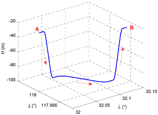
Figure 6. The sailing trajectory of the underwater vehicle.

Table 2. Motion states of the underwater vehicle.

Motions States	Time (s)
Accelerated motion	0~10
Uniform motion	10~110, 170~270, 330~430, 630~870, 1070~1170, 1230~1330, 1390~1490
Diving motion	110~170, 1330~1390
Surfacing motion	270~330, 1170~1230
Left turning motion	430~630
Right turning motion	870~1070
Decelerated motion	1490~1500

According to Section 3.1, the principle of the PLSR predictor is using s + 1 SINS calculating velocities to predict the current DVL measurement. The predictor with s + 1 SINS calculating velocities is called PLSR predictor of s + 1 steps. In order to evaluate the impact of the step number on the prediction performance, comparative simulations on PLSR predictors of different steps are carried out. It is worth mentioning that the simulations are based on the PLSR-SVR hybrid predictor, and the only difference is the step number of PLSR. Specifically, the step number is assigned the value of 2, 3, 4 and 5 respectively. To simulate the DVL malfunction, the output of the DVL is frozen from 690 s to 750 s when the underwater vehicle is in uniform motion. Here the residual chi-squared test is applied to detect the fault. Figure 7 shows the velocity errors of the system with the PLSR predictors of different steps during the fault period. Table 3 shows the evaluation of PLSR predictor of different steps.

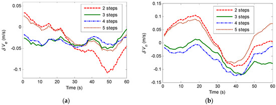
Figure 7. Velocity errors: (a) East velocity error; (b) North velocity error.

Table 3. Evaluation on PLSR predictors of different steps.

Step Number	East Velocity Error (m/s)		North Velocity Error (m/s)		Computation Consumption (s)
	Maximum	RMS	Maximum	RMS
2 steps	0.1081	0.0545	0.1249	0.0663	0.005945
3 steps	0.0514	0.0364	0.1055	0.0647	0.006277
4 steps	0.0479	0.0346	0.1196	0.0639	0.006755
5 steps	0.0561	0.0326	0.0911	0.0630	0.007651

According to Figure 7 and the maximum values of the velocity errors in Table 3, we can see that the velocity errors of the system with PLSR predictors of different steps are all within acceptable small range. Further from Table 3, the PLSR predictor of higher step performs better with smaller RMS in velocity error. However, PLSR predictor of high step means the dimension of the independent variable data matrix will be large, which will increase the computation effort. The computation consumptions of PLSR predictors of different steps are listed in the last column of Table 3. Apparently the computation consumption increases with higher step number. Considering both the prediction performance and the computation consumption, we choose PLSR predictor of 4 steps to constitute the hybrid predictor in the following simulations.

In order to further validate the performance of the proposed hybrid approach, comparative simulations with different approaches are implemented. During DVL malfunctions, the SINS/DVL/MCP/PS integrated navigation system is processed by four different solutions: (1) insulate the faulted DVL measurements without predictor (i.e., the local filter 1 introduced in Section 2.1 only executes the time update process); (2) use only PLSR predictor; (3) use radial basis function (RBF) neural network predictor [34]; (4) use PLSR-SVR hybrid predictor. It is worth noting that the DVL malfunctions listed in the introduction are all short-term, lasting for a few seconds or minutes. To simulate the sudden malfunction of the DVL, the velocity outputs of the DVL are added by 3 m/s along three directions during the period of 400~460 s when the underwater vehicle is in uniform motion and left turning motion according to Table 2. Figure 8 shows the navigation errors of the four solutions when there is a DVL malfunction for a length of 60 s.

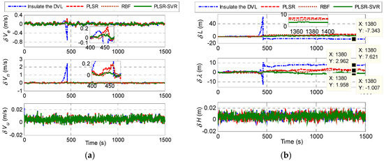
Figure 8. Navigation errors when there is a DVL malfunction for a length of 60 s: (a) Velocity errors; (b) Position errors.

Figure 8a shows that, the east and north velocity errors of the system with the first solution increase significantly during the malfunction period, which is due to the lack of external velocity information. By comparison, the systems with the other three predictors work better. Since the predictors provide the predictions of the DVL measurements, the accumulated SINS velocity errors are corrected by the prediction information. The partial enlargement drawings in Figure 8a indicate that the horizontal velocity errors of the system with the hybrid predictor are smaller than that with the PLSR predictors. This is because that the PLSR solution only establishes the linear model between the SINS calculating results and the DVL measurements. However there also exists nonlinear relationship between them (especially, for the maneuver situations). The PLSR-SVR hybrid predictor shows better accuracy by using SVR to predict the residual components of PLSR. Besides, the hybrid predictor is proved to be more effective than the RBF predictor. When the DVL failure is eliminated, the horizontal velocity errors are reduced gradually because of the available DVL velocity information. However, the latitude and longitude errors of the system have nonzero stable values as shown in Figure 8b because the horizontal position errors accumulate with the horizontal velocity errors, and the calculation for the horizontal position is an open loop. The data and the partial enlargement drawing in Figure 8b shows that the latitude errors of the systems with four different solutions stabilize at around 7.3 m, 6.9 m, 5.8 m and 3.5 m respectively, and the longitude errors stabilize around 7.6 m, 2.9 m, 2.0 m and 1 m respectively. Thus, by applying the hybrid predictor, the latitude and longitude precisions are increased by 49.3% and 65.5% respectively, in comparison with the PLSR predictor. Compared with the RBF predictor, the latitude and longitude precisions of the hybrid predictor are increased by 39.7% and 50% respectively. The advantages of the proposed hybrid predictor are apparent. As shown in Figure 8, the up velocity error and the height error of the system almost have no significant change during the malfunction period, which benefits from the external height information offered by the PS.

As we know, the performance of the predictor degrades with increasing length of malfunction. To simulate longer DVL malfunctions (more than 100 s), the outputs of the DVL along three directions are set to be zero during the period 900~1020 s when the underwater vehicle is in right turning motion. Figure 9 shows the navigation errors of the four solutions when there is a DVL malfunction for a length of 120 s. Table 4 shows the error statistics of different solutions for various DVL malfunctions.

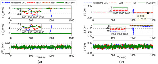
Figure 9. Navigation errors when there is a DVL malfunction for a length of 120s: (a) Velocity errors; (b) Position errors.

Table 4. Error statistics of velocity and position during DVL malfunctions.

Malfunctions Length	Solution	Absolute Maximum Velocity Error (m/s)		Absolute Maximum Position Error (m)
		East	North	Latitude	Longitude
60 s	Insulate DVL PLSR RBF PLSR-SVR	0.6869	2.438	61.03	12.92
		0.2366	0.1744	2.792	1.705
		0.1907	0.2032	4.045	1.693
		0.0793	0.0544	0.8216	1.224
120 s	Insulate DVL PLSR RBF PLSR-SVR	3.63	6.679	251.6	280.2
		0.4306	0.2311	18.69	25.49
		0.1672	0.189	12.04	20.08
		0.1261	0.1059	6.1113	8.783

According to the partial enlargement drawings in Figure 9a, the system with the hybrid predictor performs better than others during 120 s DVL malfunction. The data and the partial enlargement drawing in Figure 9b shows that the latitude errors of the systems with four different solutions stabilize at around 77.5 m, 18.7 m, 11.03 m and 5.3 m respectively, and the longitude errors stabilize at around 42.1 m, 26.6 m, 18.84 m and 7.8 m respectively. By using the hybrid predictor, the latitude and longitude precisions are increased by 71.7% and 70.7% respectively in comparison with the PLSR predictor. Compared with the RBF predictor, the latitude and longitude precisions of the hybrid predictor are increased by 51.9% and 58.6% respectively. The advantages of using the proposed hybrid predictor are more obvious in the situation of 120 s DVL malfunction than that of 60 s. It is because that the prediction precision of the other two predictors will decrease when the length of malfunction increases, but the SVR that predicts the residual components of PLSR can suppress the estimation errors to a certain extent. Consequently, the system with PLSR predictor or RBF predictor has larger horizontal position errors than the system with PLSR-SVR hybrid predictor. For both situations the hybrid predictor behaves better than the other two predictors. Based on Table 4, we can further confirm that the navigation results of the system with the PLSR-SVR predictor are superior to the other three solutions in both situations. It is worth mentioning that the position errors of the system with the proposed predictor remain less than 10 m during 120 s DVL malfunction, which is an excellent performance. Thus, it can be concluded that the hybrid predictor can effectively extend the tolerance time of the system on DVL malfunctions, which enhances the reliability and correctness of the underwater integrated navigation system.

4.2. Field Tests and Results

To further evaluate the proposed approach, the experimental data provided by the vehicle in Figure 10 is treated as the navigation data of a vehicle on the surface of the water. The experimental vehicle system includes IMU, GPS receiver and navigation computer. The reference system is an integrated navigation system consisting of a navigation-grade IMU and a GPS receiver. The reference system provides precise navigation results as reference values. The test navigation system for evaluating the proposed hybrid predictor is composed of a GPS receiver and a low-cost IMU. The specifications of the instruments in the system are listed in Table 5. The total time of the test is 500 s. Figure 11 shows the trajectory of the experimental vehicle. The vehicle travels from point A to point B.

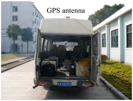
Figure 10. The experimental vehicle.

Table 5. Instrument specifications.

Instruments	Parameters	Accuracy
IMU	Gyroscope in run bias stability	0.03°/hr (1σ)
	Gyroscope angular random walk	0.005°/√hr (1σ)
	Accelerometer in run bias variation	0.2 mg (1σ)
	Accelerometer output noise	50 μg/√Hz (1σ)
GPS	Velocity	0.1 m/s
	Position	10 m

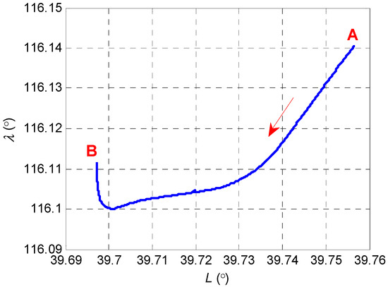
Figure 11. The trajectory of the experimental vehicle.

GPS that provides velocity information can pretend to be a DVL. To simulate a DVL malfunction for a length of 120 s, the velocity outputs of GPS are set to be zero during the period 150~270 s. Since GPS provides both velocity and position information, the position information is also employed to revise the SINS calculating results when GPS is available. In the case of malfunction, the integrated navigation system is processed by two different solutions: (1) only SINS; (2) use PLSR-SVR hybrid predictor. Figure 12 shows the navigation errors of the two solutions when there is a malfunction for a length of 120 s.

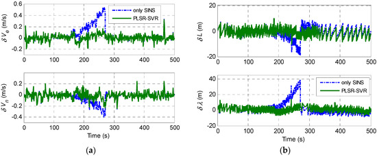
Figure 12. Navigation errors when there is a malfunction for a length of 120s: (a) Velocity errors; (b) Position errors.

Figure 12 shows that, the velocity and position errors of the system with the first solution increase during the malfunction period. Specifically, the maximum errors of east and north velocity reach to 0.546 m/s and 0.399 m/s respectively. In addition, the maximum errors of latitude and longitude reach to 18.78 m and 39.23 m respectively. By contrast, the system with the PLSR-SVR hybrid predictor acquires better accuracy on both velocity and position. Since the predictor provides the predictions of the velocity measurements, the accumulated SINS velocity errors are corrected by the prediction information. When the malfunction is removed, the position errors are corrected quickly due to the auxiliary position infromation offered by GPS. Above all, the field test results are consistent with the simulative results.

The proposed approach is validated by both simulation and field test results. Whenever a short-term DVL malfunction occurs, the hybrid predictor can immediately provide velocity information to restrain the increase of navigation errors. Therefore, the accuracy and reliability of the underwater integrated navigation system can be substantially improved.

5. Conclusions

The DVL which can be easily affected by the environment may not be able to continuously output valid measurements in complex underwater environment, so it is crucial for underwater integrated navigation systems to properly handle the DVL outages. In this paper, a hybrid predictor dealing with short-term DVL malfunctions is proposed. The hybrid approach employs PLSR and SVR to accurately predict the DVL measurements and assist the SINS to obtain accurate velocity and position information during the DVL malfunctions. More specifically, PLSR models the DVL measurements, and SVR models the residual components of the PLSR prediction. PLSR is good at dealing with the situation that strong relevance exists between the independent variables, thus it can enhance the robustness of the predictor. SVR overcomes the shortcomings of PLSR and improves the precision of the predictor. The performance of the proposed hybrid predictor is verified by comparative simulations based on SINS/DVL/MCP/PS integrated navigation system. The results show that the velocity and position errors of the navigation system can be greatly reduced by employing the PLSR-SVR hybrid predictor, compared with the other three solutions (i.e., insulating the DVL without any predictor, using only PLSR predictor and using RBF predictor). Remarkably, the position errors using the proposed hybrid prediction approach is less than 10 m for up to 120 s DVL malfunction. The field test results further validate the applicability of the proposed approach. Therefore, it is indicated that the underwater integrated navigation system with the proposed hybrid predictor can effectively deal with short-term DVL malfunctions, thereby improving the reliability and safety of underwater vehicles in complex underwater environments. Besides, the proposed hybrid prediction approach can be extended to other navigation devices, such as GPS.

References

- Negahdaripour, S.; Firoozfam, P. An ROV stereovision system for ship-hull inspection. IEEE J. Ocean. Eng. 2006, 31, 551–564. [Google Scholar] [CrossRef]
- Paull, L.; Saeedi, S.; Seto, M.; Li, H. AUV navigation and localization: A review. IEEE J. Ocean. Eng. 2014, 39, 131–149. [Google Scholar] [CrossRef]
- Ning, X.L.; Gui, M.Z.; Xu, Y.Z. INS/VNS/CNS integrated navigation method for planetary rovers. Aerosp. Sci. Technol. 2016, 48, 102–114. [Google Scholar] [CrossRef]
- Shabani, M.; Gholami, A. Improved underwater integrated navigation system using unscented filtering approach. J. Navig. 2016, 69, 561–581. [Google Scholar] [CrossRef]
- Wu, D.M.; Wang, Z.Z. Strapdown INS/GPS integrated navigation using geometric algebra. Adv. Appl. Clifford Algebras 2013, 23, 767–785. [Google Scholar] [CrossRef]
- Shabani, M.; Gholami, A.; Davari, N. Asynchronous direct Kalman filtering approach for underwater integrated navigation system. Nonlinear Dyn. 2015, 80, 71–85. [Google Scholar] [CrossRef]
- Li, D.D.; Ji, D.X.; Liu, J. A multi-model EKF integrated navigation algorithm for deep water AUV. Int. J. Adv. Robot. Syst. 2016, 13. [Google Scholar] [CrossRef]
- Hegrenaes, O.; Hallingstad, O.; Gade, K. Towards model-aided navigation of underwater vehicles. Model. Identif. Control 2007, 28, 113–123. [Google Scholar] [CrossRef]
- Tang, K.H.; Wang, J.L.; Li, W.L.; Wu, W.Q. A novel INS and Doppler sensors calibration method for long range underwater vehicle navigation. Sensors 2013, 13, 14583–14600. [Google Scholar] [CrossRef] [PubMed]
- Jalving, B.; Gade, K.; Svartveit, K. DVL velocity aiding in the HUGIN 1000 integrated inertial navigation system. Model. Identif. Control 2004, 25, 223–235. [Google Scholar] [CrossRef]
- Liu, X.X.; Xu, X.S.; Liu, Y.T.; Wang, L.H. Kalman filter for cross-noise in the integration of SINS and DVL. Math. Probl. Eng. 2014, 2014. [Google Scholar] [CrossRef]
- Li, W.L.; Zhang, L.D.; Sun, F.P.; Yang, L.; Chen, M.J.; Li, Y. Alignment calibration of IMU and Doppler sensors for precision INS/DVL integrated navigation. Optik Int. J. Electron Opt. 2015, 126, 3872–3876. [Google Scholar] [CrossRef]
- Lee, C.M.; Lee, P.M.; Hong, S.W.; Kim, S.M. Underwater navigation system based on inertial sensor and Doppler velocity log using indirect feedback Kalman filer. Int. J. Offshore Polar Eng. 2005, 15, 88–95. [Google Scholar]
- Cao, Z.Y.; Zhang, D.L.; Sun, D.J.; Yong, J. A method for testing phased array acoustic Doppler velocity log on land. Appl. Acoust. 2016, 103, 102–109. [Google Scholar] [CrossRef]
- Allotta, B.; Costanzi, R.; Meli, E. An innovative navigation strategy for autonomous underwater vehicles: An unscented Kalman filter based approach. In Proceedings of the ASME International Design Engineering Technical Conferences and Computers and Information in Engineering Conference, Boston, MA, USA, 2–5 August 2015. [Google Scholar]
- Gao, W.; Zhang, Y.; Wang, J.G. A strapdown inertial navigation system/Beidou/Doppler velocity log integrated navigation algorithm based on a cubature Kalman filter. Sensors 2014, 14, 1511–1527. [Google Scholar] [CrossRef] [PubMed]
- Mirabadi, A.; Mort, N.; Schmid, F. Fault detection and isolation in multisensor train navigation systems. In Proceedings of the UKACC International Conference on Control, Swansea, Wales, UK, 1–4 September 1998; pp. 969–974. [Google Scholar]
- Brumback, B.D.; Srinath, M.D. A fault-tolerant multisensor navigation system-design. IEEE Trans. Aerosp. Electron. Syst. 1987, 23, 738–756. [Google Scholar] [CrossRef]
- Ushaq, M.; Fang, J.C. A fault tolerant integrated navigation scheme realized through online tuning of weighting factors for federated Kalman filter. In Proceedings of the 2nd International Conference on Mechanics and Control Engineering (ICMCE 2013), Beijing, China, 1–2 September 2013; pp. 1078–1085. [Google Scholar]
- Li, X.; Zhang, W.G. An adaptive fault-tolerant multisensor navigation strategy for automated vehicles. IEEE Trans. Veh. Technol. 2010, 59, 2815–2829. [Google Scholar]
- Liang, Y.Q.; Jia, Y.M. A nonlinear quaternion-based fault-tolerant SINS/GNSS integrated navigation method for autonomous UAVs. Aerosp. Sci. Technol. 2015, 40, 191–199. [Google Scholar] [CrossRef]
- Zhao, L.Y.; Liu, X.J.; Wang, L.; Zhu, Y.H.; Liu, X.X. A pretreatment method for the velocity of DVL based on the motion constraint for the integrated SINS/DVL. Appl. Sci. 2016, 6, 79. [Google Scholar] [CrossRef]
- Semeniuk, L.; Noureldin, A. Bridging GPS outages using neural network estimates of INS position and velocity errors. Meas. Sci. Technol. 2006, 17, 2783–2798. [Google Scholar] [CrossRef]
- Hasan, A.M.; Samsudin, K.; Ramli, A.R.; Azmir, R.S. Automatic estimation of inertial navigation system errors for global positioning system outage recovery. J. Aerosp. Eng. 2011, 225, 86–96. [Google Scholar] [CrossRef]
- Belhajem, I.; Ben Maissa, Y.; Tamtaoui, A. A hybrid low cost approach using extended Kalman filter and neural networks for real time positioning. In Proceedings of the International Conference on Information Technology for Organizations Development, Fez, Morocco, 30 March–1 April 2016. [Google Scholar]
- Gilcoto, M.; Jones, E.; Busto, L.F. Robust estimations of current velocities with four-beam broadband ADCPs. J. Atmosp. Ocean. Technol. 2009, 26, 2642–2654. [Google Scholar] [CrossRef]
- Adusumilli, S.; Bhatt, D.; Wang, H.; Devabhaktuni, V.; Bhattacharya, P. A novel hybrid approach utilizing principal component regression and random forest regression to bridge the period of GPS outages. Neurocomputing 2015, 166, 185–192. [Google Scholar] [CrossRef]
- Al-Alawi, S.M.; Abdul-Wahab, S.A.; Bakheit, C.S. Combining principal component regression and artificial neural networks for more accurate predictions of ground-level ozone. Environ. Model. Softw. 2008, 23, 396–403. [Google Scholar] [CrossRef]
- Wold, S.; Albano, C.; Dunn, M.; Esbensen, K.; Hellberg, S.; Johansson, E. Pattern Regression Finding and Using Regularities in Multivariate Data; Analysis Applied Science Publication: London, UK, 1983. [Google Scholar]
- Samkar, H.; Guven, G. Comparison of PLSR and PCR techniques in terms of dimension reduction: An application on internal migration data in Turkey. Int. J. Adv. Appl. Sci. 2016, 3, 7–13. [Google Scholar] [CrossRef]
- Cortes, C.; Vapnik, V. Support-vector networks. Mach. Learn. 1995, 20, 273–297. [Google Scholar] [CrossRef]
- Kavousi-Fard, A.; Samet, H.; Marzbani, F. A new hybrid modified firefly algorithm and support vector regression model for accurate short term load forecasting. Expert Syst. Appl. 2014, 41, 6047–6056. [Google Scholar] [CrossRef]
- Cheng, C.H.; Yang, J.H. A novel rainfall forecast model based on the integrated non-linear attribute selection method and support vector regression. J. Intell. Fuzzy Syst. 2016, 31, 915–925. [Google Scholar] [CrossRef]
- Pang, C.P.; Liu, Z.Z. Bridging GPS outages of tightly coupled GPS/SINS based on the adaptive track fusion using RBF neural network. In Proceedings of the IEEE International Symposium on Industrial Electronics, Seoul, Korea, 5–8 July 2009. [Google Scholar]
© 2017 by the authors. Licensee MDPI, Basel, Switzerland. This article is an open access article distributed under the terms and conditions of the Creative Commons Attribution (CC BY) license (http://creativecommons.org/licenses/by/4.0/).