Development and Application of a “Decomposition–Denoising”-Based Vibration-Signal Denoising System for Radial Steel Gates Under Discharge Excitation

Abstract

To mitigate the pervasive noise interference present in the measured vibration signals of radial steel gates and to address the limitations of conventional wavelet-threshold denoising, this study proposes a coupled “decomposition–denoising” theoretical framework for vibration-signal purification. The key novelty lies in a smooth and tunable thresholding strategy that enables controlled filtering while preserving key structural characteristics within an integrated denoising workflow. In the proposed approach, the measured signal is decomposed into intrinsic mode components using a data-driven decomposition method, noise-dominated components are identified using multiscale permutation entropy, and only these components are selectively denoised before signal reconstruction. Both qualitative and quantitative analyses conducted on synthetic signals demonstrate the effectiveness of the proposed framework and confirm the enhanced smoothness and robustness of the improved thresholding scheme. Performance is evaluated using objective measures such as signal-to-noise ratio and root-mean-square error, together with spectral-consistency checks for field measurements. Furthermore, two field-measured engineering cases involving radial steel gates substantiate the engineering applicability and generalization capability of the proposed method, showing clearer signals and more stable diagnostic-relevant indicators. Finally, the study integrates the decomposition, denoising, and parameter-selection modules into a user-oriented vibration-signal denoising system, establishing an efficient workflow for engineering signal processing and subsequent structural-health monitoring applications.

1. Introduction

As a controllable and renewable energy source, hydropower has been extensively developed worldwide owing to its sustainability and environmental friendliness, playing a vital role in achieving carbon-neutral energy transitions [1,2]. During hydropower station operation, the arch-type steel gate regulates flow discharge by adjusting its opening, ensuring safe and stable water management. However, the gate is subjected to unsteady hydrodynamic excitations during discharge, operating in harsh conditions. A gate malfunction or failure under such circumstances can cause severe downstream property losses and even threaten human safety, while also compromising the economic performance of the hydraulic infrastructure [3]. To monitor its dynamic characteristics, acceleration sensors are typically installed on major load-bearing components such as gate arms and main girders to measure the root-mean-square (RMS) vibration during discharge and to extract vibration features for dynamic assessment [4]. Beyond centralized/offline postprocessing, recent studies have highlighted the trend of implementing signal preprocessing and diagnostic-metric stabilization directly at the measurement-system edge (embedded or smart controllers), which can reduce latency and bandwidth demand and improve the robustness of operational indicators. For example, Landar et al. reported a Smart 4 controller for assessing bottom-part drill-string vibrations and shock loads, demonstrating the value of near-sensor processing for vibration/shock evaluation [5]. Velychkovych et al. further discussed threshold-type vibration metrics derived from field trials to interpret tool wear and penetration-rate degradation, illustrating how preprocessing and metric design directly affect the stability and interpretability of diagnostic indicators [6]. Together, these studies highlight a broader trend in vibration monitoring: preprocessing and metric design near the sensor can directly influence the reliability of condition assessment. These developments support the practical relevance of developing application-oriented denoising workflows and reproducible processing systems for hydraulic gate vibration monitoring.

In gate-operation monitoring, the dynamic response signals acquired by sensors are often affected by multiple sources—such as flow pulsation, structural vibration, ambient disturbances, and measurement errors—exhibiting significant randomness and non-stationarity [7,8]. The presence of noise not only obscures the true dynamic behavior of the structure but also degrades the accuracy of subsequent modal identification, condition evaluation, and fault diagnosis. Therefore, developing efficient and robust noise-suppression methods is of great importance for enhancing the reliability of gate operation monitoring [9,10].

Existing signal-denoising techniques can generally be divided into two categories. The first category, direct denoising methods, includes wavelet thresholding, adaptive filtering, empirical spline smoothing, and variational denoising. These approaches achieve signal smoothing and noise reduction through thresholding, filtering, or regularization, offering advantages such as computational simplicity and real-time capability. However, when dealing with multiscale, nonlinear, and strongly non-stationary signals, their performance is highly sensitive to the selected threshold model or filter parameters, often resulting in over-smoothing, detail loss, and edge distortion [11,12]. The second category consists of decomposition-based noise-suppression methods, which decompose complex signals into multiple scale-distinct components and then reconstruct the signal after identifying noisy and clean modes using statistical indicators such as permutation entropy [13], kurtosis [14], or correlation coefficients [15]. The development of decomposition algorithms has undoubtedly opened new avenues for noise reduction. Since Huang et al. (1998) introduced empirical mode decomposition (EMD) [16], numerous improvements have been proposed to address issues such as mode mixing, end effects, and incomplete reconstruction. Ensemble EMD (EEMD) mitigates mode mixing through a noise-assisted averaging mechanism but remains sensitive to the amplitude and iteration number of the added noise [17]. Complementary EEMD (CEEMD) [18] and CEEMDAN [19] further enhance energy conservation and mode orthogonality, though at the expense of higher computational cost and empirically tuned noise weights. Later, improved CEEMDAN (ICEEMDAN) [20] introduced dynamic noise scaling during iterations, effectively eliminating reconstruction errors and yielding IMFs with stronger physical interpretability. In parallel, variational mode decomposition (VMD) reformulated signal decomposition as a variational optimization problem, enabling strict mathematical control over the bandwidth of each mode and eliminating mode mixing [21]. These methods have been widely validated across domains: Zhao [22] used EMD combined with filtering for gyroscope signal denoising; Zvokelj [23] employed EEMD for vibration–acoustic emission signals in bearing tests; and Zhang [24], Li [25], and Athisayam [26] applied CEEMD with deep learning or hybrid methods for denoising laser Doppler, coal-loading temperature, and turning vibration signals, respectively. Similarly, Peng [27], Zhou [28], Zheng [29], Zhang [30], Yin [31], and Fan [32] combined CEEMDAN with various algorithms for denoising underwater blasting, vibration, UAV magnetic, turbine acoustic, micro-seismic, and lidar echo signals, all with promising results. Lu [33] and Wei [34] adopted VMD-based denoising for hydraulic gate and turbine current signals, while ICEEMDAN-based methods demonstrated superior performance in mechanical vibration [35], acoustic [36,37], and micro-seismic [38] signal denoising. These advances underscore the increasing significance of decomposition-based strategies in signal purification.

Nevertheless, decomposition algorithms also face parameter sensitivity issues. Their performance strongly depends on key parameters: in VMD, the number of modes (K) and penalty factor (α) control modal resolution and bandwidth compactness, where improper selection may lead to component leakage, pseudo-modes, or excessive smoothing [39,40]. Similarly, the effectiveness of EEMD, CEEMD, CEEMDAN, and ICEEMDAN is affected by the noise amplitude weight (Nstd) and number of noise realizations (NE) [41]. In recent years, researchers have introduced intelligent optimization algorithms to achieve adaptive parameter tuning and improve robustness under complex noise conditions. For instance, Cao [42], Wu [43], Fan [44], Cheng [45], and Cao [46] optimized the parameters of VMD using algorithms such as IPSO, WOA, CPO, ISOA, and NRBO for denoising lidar, transformer discharge, underwater acoustic, pump impeller, and ultrasonic echo signals, respectively. Zhang [47] further applied WOA to optimize ICEEMDAN parameters (Nstd and NR) for ultrasonic echo denoising. These studies have established a solid theoretical and practical foundation for the integration of optimization algorithms with decomposition-based denoising.

Regarding IMF component classification, single-scale statistical indices often exhibit poor stability and generalization in non-stationary, cross-scale hydraulic vibration environments, being highly sensitive to window length, local discontinuities, and transient disturbances. To address this, the present study adopts an improved multiscale permutation entropy (MPE) approach. By constructing coarse-grained multiscale time series and computing entropy across scales, MPE captures the intrinsic complexity–scale relationship of IMFs [48,49]. Moreover, since noisy components may still contain useful structural information, the direct elimination of IMFs can lead to information loss and waveform distortion. Thus, noisy IMFs are denoised rather than discarded and then superposed with clean IMFs to ensure signal integrity upon reconstruction. Among denoising techniques, wavelet thresholding remains widely applied due to its adaptability and efficiency. However, traditional hard thresholding introduces discontinuities at the threshold, causing ringing and artifacts, while soft thresholding, though continuous, is non-differentiable at the threshold and introduces bias for large coefficients—resulting in detail attenuation and limited differentiability for subsequent gradient-based optimization [11,12]. To overcome these shortcomings, this study proposes an improved, continuously differentiable shrinkage function that enhances smoothness around zero for stronger noise suppression, approximates identity mapping in large-amplitude regions, and employs a tunable smoothness parameter to balance bias and variance. This modification mitigates ringing and boundary artifacts induced by discontinuity, alleviates the soft-threshold bias and “staircase effect,” and significantly improves the fidelity of transient and modal details without altering the decomposition or thresholding framework.

Finally, in complex monitoring environments, the inherent non-stationarity, multiscale behavior, transient nonlinearities, and time-varying SNR of hydraulic gate signals imply that no single decomposition method can be universally optimal. Different methods embody distinct inductive biases and assumptions (e.g., VMD is well suited for narrowband components, while EMD-based methods better capture nonlinear trends but are sensitive to mode mixing and parameter perturbations). Their performance remains strongly dependent on hyperparameter-noise structure compatibility. Therefore, from both methodological and engineering perspectives, this study develops an integrated multi-algorithm denoising system that unifies VMD, EMD, CEEMDAN, and ICEEMDAN under a modular framework. The system enables adaptive hyperparameter optimization via intelligent algorithms, integrates MPE-based component discrimination, and provides multiple selectable wavelet-thresholding options with improved differentiability. This framework constitutes a comprehensive and efficient denoising platform, supporting researchers and engineers in robust signal preprocessing for subsequent analysis and decision-making. To avoid any ambiguity regarding the relationship between this manuscript and our previous publication in Applied Sciences [33], we clarify that the earlier work primarily focused on optimization-driven VMD parameter selection (e.g., MVO-optimized K and α) and its combination with conventional wavelet-threshold denoising for spillway radial-gate signals. In contrast, the present study is positioned as a more general “decomposition–denoising” workflow and emphasizes a continuously differentiable, smooth and tunable thresholding scheme, together with an application-oriented denoising system that supports multiple decomposition options, component selection, selective denoising, and reproducible field deployment.

2. Data and Method

2.1. Data Acquisition

After validating the proposed method using physical signal tests, further verification was conducted to demonstrate the applicability of the joint denoising theory in practical engineering scenarios. Two representative cases were analyzed: the field observation of a surface-bay radial gate and the flow-induced vibration model test of a deep-bay radial gate.

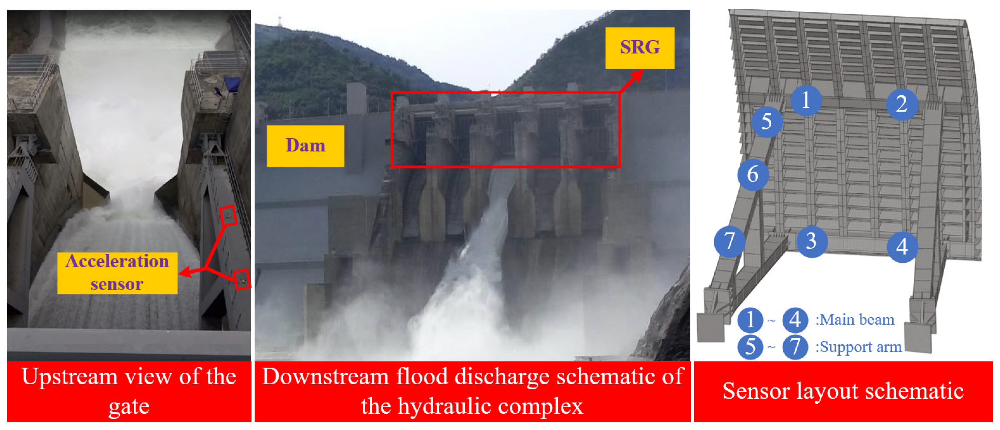
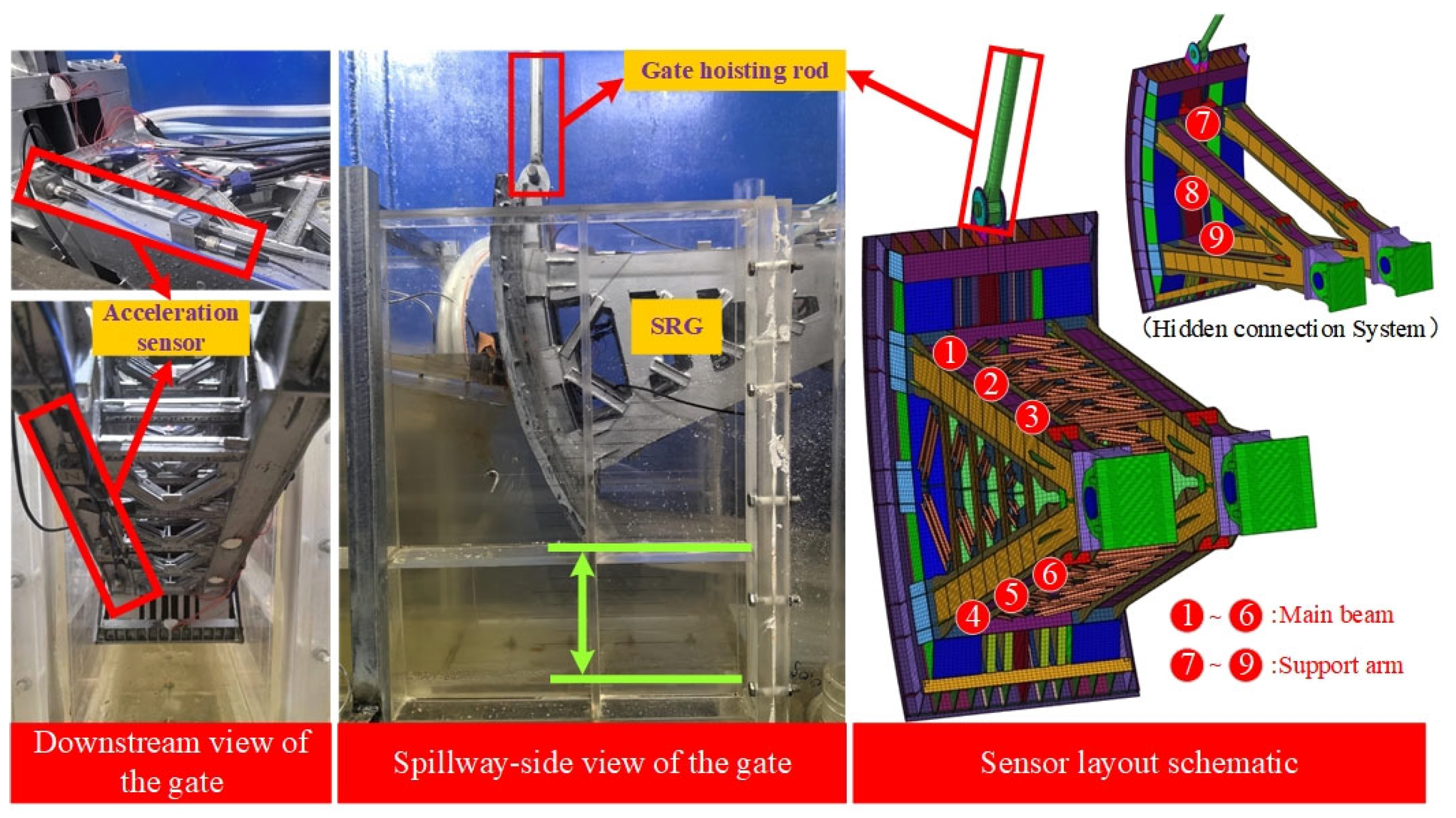
Project A is located in the Yalong River Basin in southwestern China and represents an operational hydraulic hub project whose spillway structure adopts a surface-bay radial-gate configuration. The gate features a “main crossbeam–dual arm” frame arrangement. To capture the dynamic response characteristics of the gate under flood discharge conditions, multiple vibration-acceleration sensors were installed on both the gate leaf and its supporting arms. Two tri-axial accelerometers were mounted on the upper and lower main crossbeams of the gate leaf to measure vibrations in the tangential, radial, and lateral directions. Additionally, three tri-axial accelerometers were placed on the upper-left arm to measure vibrations in the axial, vertical, and lateral directions. This instrumentation layout enabled comprehensive monitoring of the gate’s vibrational behavior at different structural locations and directions during partial opening operations under hydrodynamic loading. The tri-axial accelerometers used in the test were of the LC01 series manufactured by Langsi Testing Technology Co., Ltd. (Qinhuangdao, China). The data acquisition system employed the INV-series intelligent signal-acquisition instrument produced by Beijing Oriental Company (Beijing, China), together with the DASP-V11 data acquisition and analysis software for signal recording and processing.

The gate’s sensor layout and discharge conditions are illustrated in Figure 1.

Project B is a hydraulic engineering project currently under construction in the Lancang River Basin, southwestern China. The project’s spillway gates are deep-hole radial gates designed for flood discharge, featuring a structural frame composed of one main longitudinal beam and two supporting arms. Since the project is still under construction, a flow-induced vibration model test was conducted. The prototype gate is made of Q345B structural steel with an elastic modulus E ≈ 206 GPa. According to the hydro-elastic similarity requirements, an appropriate model material was selected. By using an organic composite material combined with a density-enhancing filler and by adjusting the formulation and manufacturing process, both the density and elastic modulus were tuned to satisfy the elastic similarity criteria. The finally selected material has an elastic modulus of 8.24 GPa and a unit weight of 7.8 kN/m³. Single-axis accelerometers were installed on the upper, middle, and lower crossbeams of the gate to measure the radial vibration of the gate leaf. In addition, three tri-axial accelerometers were mounted on the upper-left and lower-left arms of the gate to record vibrations in the axial, vertical, and lateral directions. The vibration measurements employed Donghua 1A314E accelerometers (Taizhou, China), with data acquisition performed via a cDAQ-9189 modular chassis (National Instruments, Austin, TX, USA). The acceleration acquisition module used was the NI 9230 analog voltage input module (National Instruments, Austin, TX, USA), capable of measuring various IEPE/ICP-type sensor signals.

The sensor arrangement on the gate and the flow-discharge condition are illustrated in Figure 2.

2.2. Decomposition Methods

2.2.1. EMD Family

Empirical mode decomposition (EMD) and its noise-assisted variants provide a data-driven decomposition of nonlinear and non-stationary signals into a finite set of intrinsic mode functions (IMFs) and a residual trend. Because the EMD family is well established, we omit textbook-level derivations here and refer readers to standard references for algorithmic details. Noise-assisted ensemble variants (e.g., EEMD and the complete ensemble forms CEEMDAN/ICEEMDAN) are widely used to improve the stability of IMF extraction and mitigate mode mixing under strong interference [16,17,18,19,20].

In this study, EMD-family decomposition is used as a decomposition front-end within the proposed “decomposition–denoising” workflow. The extracted IMFs are subsequently evaluated by multiscale permutation entropy (MPE) and selectively denoised prior to reconstruction, enabling noise suppression while retaining key structural characteristics.

2.2.2. VMD

Variational mode decomposition (VMD) is a variational, optimization-based decomposition technique that represents a signal as a pre-defined number of band-limited modes. Compared with EMD-type approaches, VMD formulates decomposition as a constrained optimization problem and can provide stable mode extraction in practical applications. Since VMD is a well-established method, we do not repeat the textbook derivations here and refer readers to standard references for algorithmic details [21].

In this study, VMD is integrated as an alternative decomposition module within the proposed “decomposition–denoising” system. After decomposition, the resulting modes are processed by the same subsequent steps (component evaluation/selection and selective denoising) to ensure a unified workflow. The key VMD parameters include the number of modes K and the penalty factor α, which are set consistently with the unified experimental configuration to maintain comparability across different decomposition choices.

2.3. Classification Criteria

Multiscale permutation entropy (MPE) extends the ordinal complexity measure of permutation entropy (PE) by introducing a coarse-graining procedure across multiple temporal scales. It characterizes the ordinal structure and uncertainty of non-stationary time series over different time scales. Unlike amplitude-based measures, MPE focuses on the relative ordering among data points rather than their absolute magnitudes, rendering it invariant to amplitude translation, scaling, and any strictly monotonic transformation. Moreover, it reveals the evolution of dynamical complexity from short-term microscopic to long-term macroscopic behaviors across scales.

For a given scalar sequence $x={\left\{x_t\right\}}_{t=1}^N$ with embedding dimension m and time delay τ, the delayed embedding vectors are constructed as

$${\mathrm{v}}_i=(x_i,x_{i+\tau },\dots ,x_{i+(m-1)\tau })\in {ℝ}^m,i=1,\dots ,N-(m-1)\tau$$

(1)

The components of v_i are arranged in ascending order, and the resulting index sequence is encoded as a pattern label k_i ∈ {1,…, m!}.

The empirical probability of the k-th ordinal pattern is then defined as

$$p_k={\displaystyle \frac{1}{N^{\prime }}}{\displaystyle \sum _{i=1}^{N^{\prime }}I(k_i=k)},k=1,\dots ,m!$$

(2)

where I( ) is the indicator function, which equals 1 if the condition is true and 0 otherwise.

The permutation entropy is then defined as

$$P{E}_{m,\tau }(x)=-{\displaystyle \sum _{k=1}^{m!}{p}_k\ln p_k}$$

(3)

Multiscale permutation entropy (MPE) extends the conventional permutation entropy by introducing a multiscale procedure, enabling the analysis of the dynamical characteristics of time series across different temporal scales. The specific steps are as follows:

(1)

Multiscale process: The coarse-grained time series is constructed from the original sequence.

Given a time series ${\left\{x_i\right\}}_{i=1}^N$ and a scale factor s, the coarse-grained series is defined as

$$y_j^{(s)}={\displaystyle \frac{1}{s}}{\displaystyle \sum _{i=(j-1)s+1}^{js}{x}_i},j=1,2,\dots ,\left[{\displaystyle \frac{N}{s}}\right]$$

(4)

(2)

Computation of permutation entropy at different scales: For each scale (s), the permutation entropy (PE(s)) of the corresponding coarse-grained time series $\left\{y_j^{(s)}\right\}$ is calculated following the standard procedure of permutation entropy.

(3)

Definition of multiscale permutation entropy: The MPE is defined as the collection of permutation entropy values obtained across all scales, i.e.,

$$MPE=\left\{PE(s)\left|s=1,2,\dots ,S\right.\right\}$$

(5)

where S denotes the maximum scale factor.

In practice, the MPE-based discrimination requires a threshold to separate noise-dominated and information-dominated components. Following commonly adopted empirical settings in entropy-based IMF/component classification studies, the threshold is set to 0.6 as the default in this work [33,50,51]. This threshold is user-configurable in the developed denoising system and can be adjusted according to signal characteristics and engineering requirements. It is also noted that, in the proposed workflow, IMFs classified as noise-dominated are selectively denoised rather than discarded and then recombined with the preserved IMFs during reconstruction. This design reduces the risk of inadvertently removing physically meaningful dynamics when operating regime change, while still enabling effective suppression of noise-contaminated components.

2.4. Improved Wavelet-Threshold Denoising Theory

The core of wavelet-threshold denoising lies in the design of the threshold function and the selection of its parameters. Conventional hard- and soft-threshold functions suffer from discontinuity and constant bias, respectively. To address these issues, this study proposes a target-attenuation-controlled smooth threshold function, defined as

$$f(x)=\left\{\begin{array}{l}\mathrm{sign}(x)(\left|x\right|-{\displaystyle \frac{2T}{\exp (\frac{\left|x\right|-T}{\alpha T})+1}}),\left|x\right|>T\\ 0,\left|x\right|\le T\end{array}\right.$$

(6)

This function is continuous and differentiable at |x| = T. This differentiability improves numerical stability and makes the thresholding module compatible with gradient-based optimization frameworks; however, the present study adopts the rule-based parameter configuration described below rather than derivative-based tuning. The parameter α controls the transition bandwidth between strong shrinkage and near-identity mapping: a smaller α yields a steeper transition (hard-threshold-like), whereas a larger α produces a smoother transition (soft-threshold-like).

To eliminate the empirical dependency of α, a target-attenuation criterion is introduced: at a reference amplitude |x| = mT (m > 1), the output is constrained to exhibit only a relative attenuation ρ ∈ (0, 1), i.e.,

$$f(mT)=(1-\rho )mT$$

(7)

Substituting the above into f(x) yields

$$mT-{\displaystyle \frac{2T}{\exp (\frac{m-1}{\alpha })+1}}=(1-\rho )mT$$

(8)

Solving yields the closed-form analytical expression for the smoothing parameter:

$$\alpha ={\displaystyle \frac{m-1}{\ln (\frac{2}{m\rho }-1)}}$$

(9)

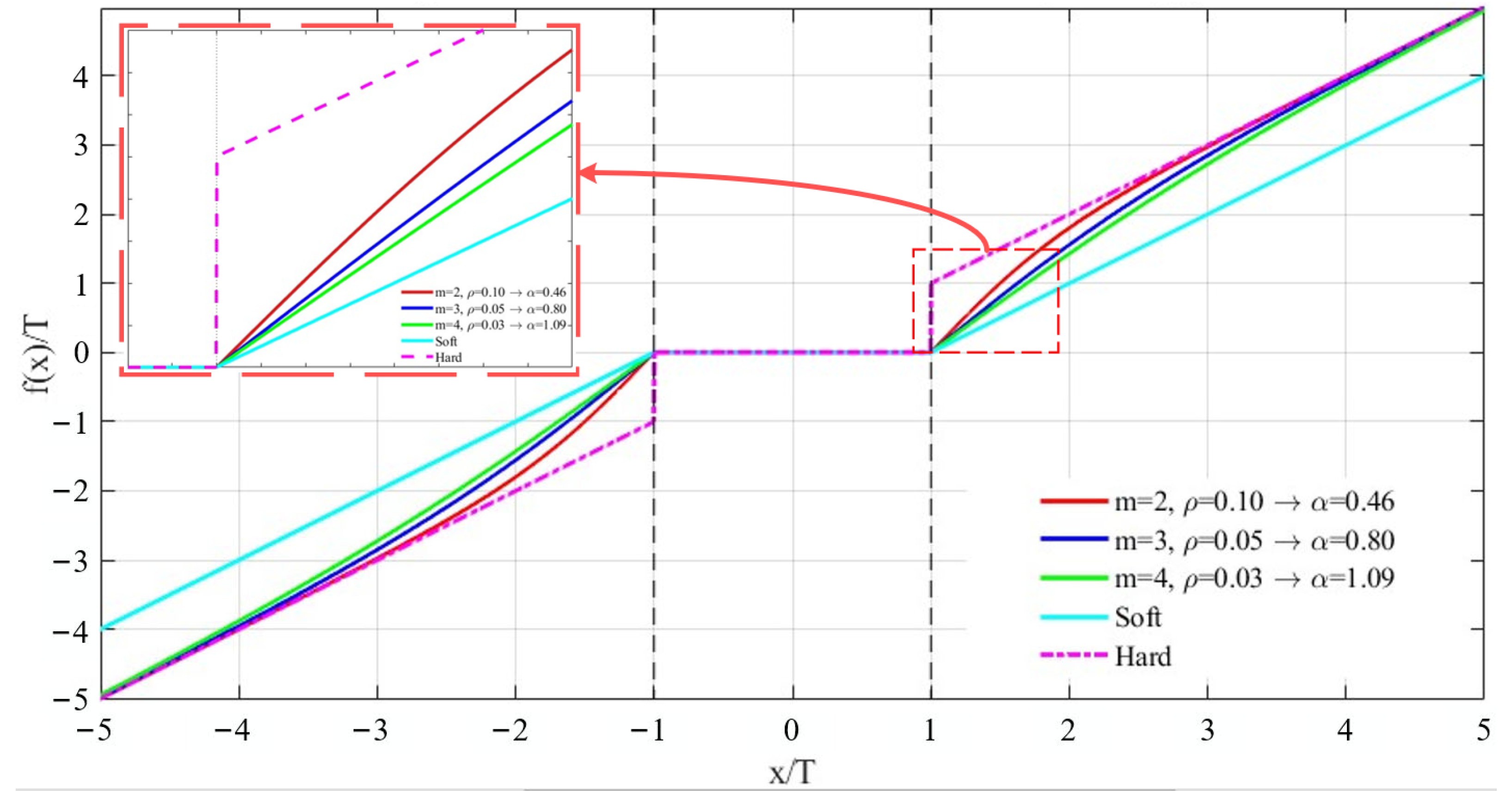
The parameter m defines the reference position to ensure that the signal attenuation does not exceed a specified ratio, while the parameter ρ sets the target-attenuation ratio, determining the degree of amplitude reduction. Together, these parameters determine the smoothing index α, which can be flexibly adjusted in a reproducible manner according to the noise characteristics of the signal. The comparison between the improved threshold function curve and the traditional soft and hard threshold curves is shown in Figure 3.

As illustrated in Figure 3, the improved threshold function proposed in this study establishes a smooth transition mechanism between the conventional soft and hard thresholds. By introducing a shape-control parameter m and a scaling factor ρ, the constant bias of wavelet coefficients is further suppressed. Compared with the soft threshold, the improved function avoids excessive shrinkage in the low-amplitude region; in contrast to the hard threshold, it eliminates discontinuities at the threshold point, thereby achieving low-bias and continuously differentiable characteristics. These properties enhance the smoothness and structural fidelity of the denoised signal. In general, (m, ρ) = (3, 0.05) can be used as the baseline configuration, for which the corresponding α ≈ 0.83, comparable to several smooth-type threshold functions such as FirmShrink, SmoothShrink, and exponential-decay variants. This setting offers a desirable trade-off between denoising performance and signal fidelity. This setting offers a desirable trade-off between denoising performance and signal fidelity. In this study, the baseline configuration and the recommended ranges in

Table 1. Recommended parameter ranges under different noise levels.

Signal Type	Noise Level	Suggested Parameters	α Range	Characteristic Description
High noise	SNR < 10 dB	m = 2.0–2.5, ρ = 0.10	α ≈ 1.0–1.2	Smooth transition; strong denoising but slightly soft response
Medium noise	SNR ≈ 10–20 dB	m = 3.0, ρ = 0.05	α ≈ 0.8	Balanced denoising and fidelity
Low noise	SNR > 20 dB	m = 4.0, ρ = 0.03	α ≈ 0.65	Strong peak preservation; slightly hard profile

are adopted to ensure reproducibility across comparisons. The recommended parameter ranges under various noise levels are summarized in Table 1, where typical signal types, suggested parameter combinations, and their characteristic descriptions are provided as practical guidance for parameter selection. Derivative-based end-to-end tuning will be explored in future work.

2.5. Technical Roadmap

The theoretical framework and software development workflow of the proposed joint denoising approach are as follows.

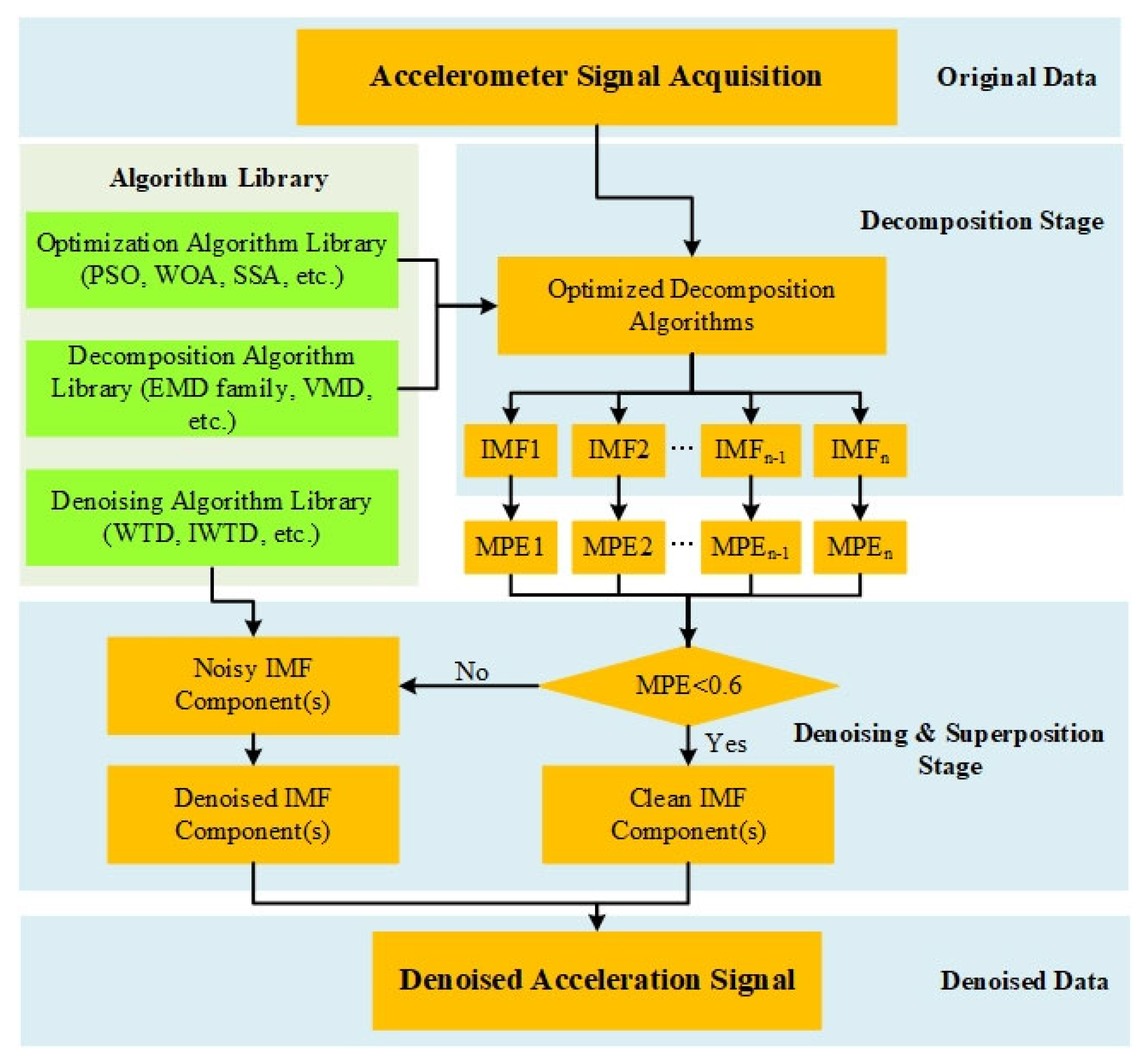
From the overall process perspective, the noisy signal is first decomposed into a series of intrinsic mode function (IMF) components. Then, the multiscale permutation entropy (MPE) of each IMF is computed, based on which the components are classified into clean and noisy groups. The noisy components are subsequently denoised using either the conventional wavelet thresholding or the proposed improved wavelet-thresholding method, yielding the denoised IMFs. Finally, the denoised components are superimposed with the clean ones to reconstruct the overall denoised signal. In terms of system implementation, the denoising module is encapsulated according to the above framework. The decomposition module integrates the EMD family of algorithms (EMD, EEMD, CEEMD, CEEMDAN, ICEEMDAN) as well as the VMD algorithm. For key algorithmic parameters—such as the noise standard deviation (NSTD) and ensemble size (NE) in EEMD/CEEMD, the NSTD, NE, and MaxIter in CEEMDAN/ICEEMDAN, and the decomposition level K and penalty factor α in VMD—the system incorporates multiple intelligent optimization algorithms (WOA, SAO, CWO, SSA, PSO, etc.) to achieve adaptive parameter tuning. The overall technical workflow of the proposed joint denoising framework is illustrated in Figure 4.

3. Synthetic Signal Simulation

3.1. Synthetic Signal

To evaluate the performance of the proposed denoising algorithm, an artificial simulation signal is first employed to verify the effectiveness of the method. The artificial signal is defined as follows:

$$\left\{\begin{array}{l}y=x_1+x_2+x_3+x_{noise}\\ x_1=0.2\cos (2\pi t)\\ x_2=0.5\sin (5\pi t)\\ x_3=0.4\sin (8\pi t)\\ x_{noise}=0.5randn\left(N,1\right)\end{array}\right.$$

(10)

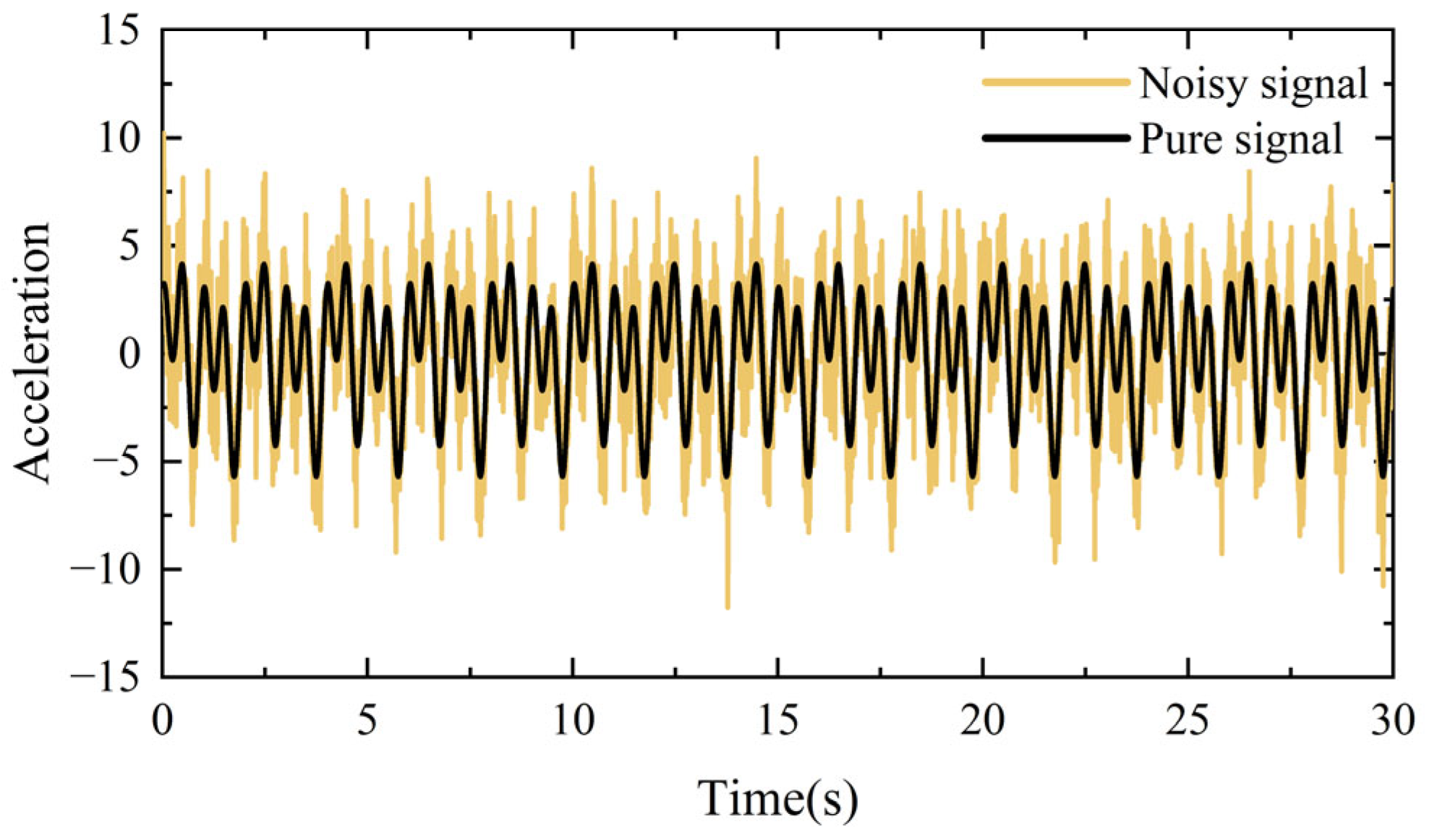
where x_noise represents the random white noise signal, y is the noise-contaminated synthetic signal, and y-x_noise = x₁ + x₂ + x₃ corresponds to the clean signal. The waveforms of the clean and noise-contaminated signals are shown in Figure 5.

From the comparison of the pre- and post-denoising results, it can be observed that after noise is added to the clean signal, the signal trend becomes irregular, and the noise overwhelms the original waveform, making it difficult to distinguish the underlying signal pattern.

3.2. Evaluation of Joint Denoising Performance on Synthetic Signals

Given the limitation of space, the VMD algorithm and the representative EMD algorithm from the EMD family were selected to construct two typical decomposition-based joint denoising schemes—VMD-MPE-IWTD and EMD-MPE-IWTD—for denoising validation using artificially noise-contaminated signals. In addition, to verify the effectiveness of the optimization algorithms, the VMD algorithm was used as an example to demonstrate the optimization performance.

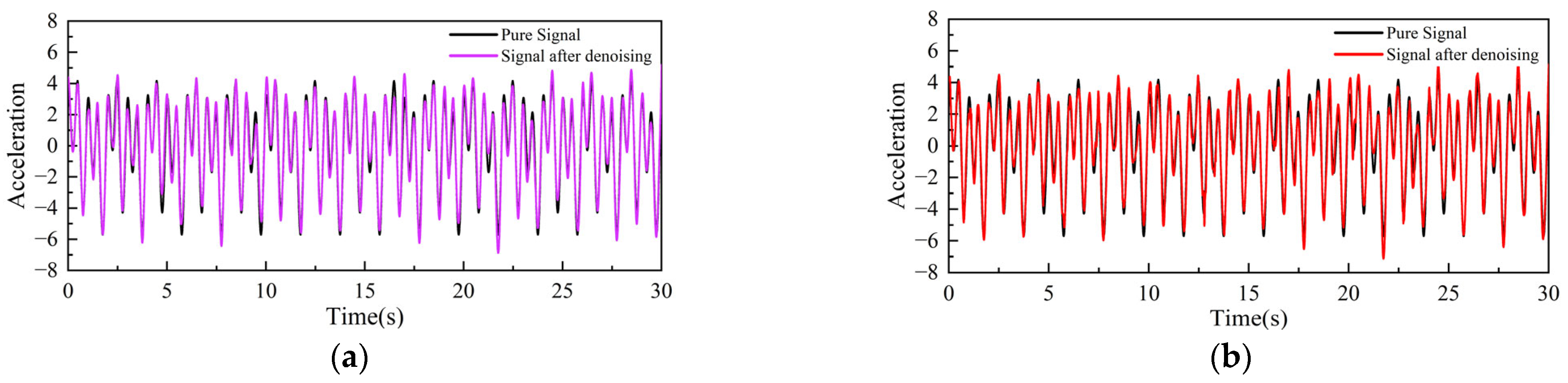
The time–history waveforms before and after denoising are shown in Figure 6. It can be observed that, after applying the proposed joint denoising method, the processed signal exhibits a high degree of waveform consistency and trend agreement with the original signal, indicating that the method effectively suppresses noise while preserving the primary features of the signal.

To quantitatively evaluate the effectiveness of each denoising algorithm further, the signal-to-noise ratio (SNR) and root mean squared error (RMSE) are compared for the discrete-time benchmark signals with a known clean reference. It should be emphasized that SNR and RMSE are used only for benchmark signals with a known clean reference. For field-measured gate responses, a truly noise-free reference is unavailable; therefore, absolute SNR/RMSE is not applicable and not used for field parameter tuning or evaluation. SNR is a key indicator of signal quality, reflecting the relative intensity between signal energy and noise energy; a higher SNR value indicates a more effective noise-suppression performance. RMSE measures the average deviation between the denoised signal and the clean reference signal, providing an intuitive assessment of reconstruction accuracy; a smaller RMSE value corresponds to better denoising performance. Under noise-contaminated conditions, the input SNR of the original signal is approximately 4.4624 dB.

To ensure comparability across methods, all control variables were configured consistently. For noise-assisted decomposition algorithms (EEMD, CEEMD, CEEMDAN, and ICEEMDAN), the noise amplitude Nstd was set to 0.05, and the ensemble size NE was fixed at 100. For CEEMDAN and ICEEMDAN, the maximum number of sifting iterations per IMF (MaxIter) was set to 20. It is worth noting that the standard EMD algorithm does not involve noise addition; thus, the parameter Nstd is not applicable to EMD. For each benchmark case, a single noise realization is generated and kept fixed across all compared methods to ensure fair and reproducible comparisons. Under the above unified configuration, the statistical results of denoising performance for all methods are summarized in

Table 2. Statistical results of denoising performance for EMD-family decomposition algorithms (benchmark signals with a known clean reference; metrics: SNR and RMSE).

	SNR	RMSE		SNR	RMSE
WTD	8.4118	1.2522	IWTD	14.2917	0.63632
EMD-MPE-WTD	10.7832	0.9944	EMD-MPE-IWTD	14.6856	0.596
EEMD-MPE-WTD	10.7089	0.9612	EEMD-MPE-IWTD	14.6614	0.59811
CEEMD-MPE-WTD	10.4618	0.98894	CEEMD-MPE-IWTD	15.3894	0.56078
CEEMDAN-MPE-WTD	10.5744	0.9762	CEEMDAN-MPE-IWTD	14.7859	0.60113
ICEEMDAN-MPE-WTD	10.6956	0.96267	ICEEMDAN-MPE-IWTD	14.8624	0.59586

.

From an overall perspective, the introduction of the decomposition–reconstruction joint strategy results in a significant improvement in SNR and a marked reduction in RMSE, indicating that the proposed joint denoising approach can effectively suppress noise while better preserving the intrinsic features of the signal.

Taking the conventional wavelet-threshold denoising (WTD) method as a baseline, its SNR and RMSE are 8.41 dB and 1.25, respectively. After incorporating modal decomposition and multiscale permutation entropy (MPE)-based component discrimination, the EMD-MPE-WTD method increases the SNR to 10.78 dB—an enhancement of approximately 28.2%—and reduces the RMSE by about 20.6%. A comparison between the traditional and the improved wavelet-thresholding (IWTD) approaches further demonstrates that IWTD consistently outperforms WTD across all decomposition frameworks. This improvement confirms that the modified threshold function effectively overcomes the non-differentiability and over-shrinkage issues inherent in conventional soft and hard thresholds, yielding smoother and more accurate reconstructed signals.

Among the various decomposition algorithms, EEMD, CEEMD, CEEMDAN, and ICEEMDAN achieve slightly superior results compared with the basic EMD method, primarily due to their enhanced capability in alleviating mode mixing and stabilizing the intrinsic mode function (IMF) extraction process. In the case of variational mode decomposition (VMD), the decomposition level K and penalty factor α are the key parameters governing both decomposition quality and denoising performance. Since these parameters must be pre-defined, their values directly influence the frequency-band partitioning and energy distribution of the resulting modes, thereby determining the overall quality of signal reconstruction. If K is too small, signals from different frequency bands may overlap, causing mode mixing; conversely, an excessively large K may lead to mode redundancy and a substantial increase in computational cost. Similarly, a large penalty factor α may result in over-smoothed components that lose signal detail, whereas a small α may cause non-smooth or oscillatory solutions. Hence, the appropriate selection of optimal K and α is a critical issue in practical VMD applications.

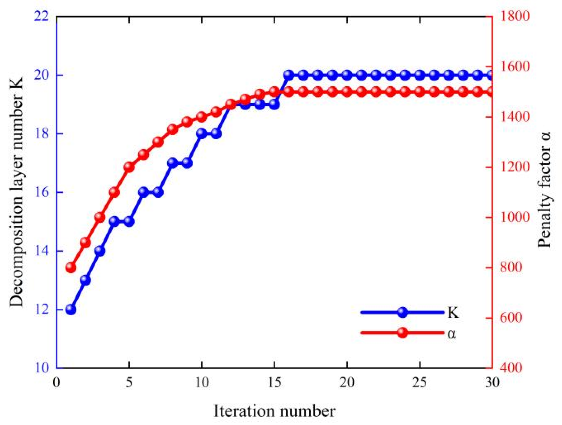
With the advancement of intelligent optimization techniques, population-based global search algorithms have provided new insights into the adaptive determination of VMD parameters. In this study, the whale optimization algorithm (WOA) is introduced for the benchmark signals, using SNR as the objective function to adaptively optimize K and α. For field measurements, the VMD parameters follow the recommended/rule-based configuration, and field performance is assessed using dnSNR (Equations (11)–(13)) and dominant spectral-consistency checks, rather than absolute SNR/RMSE. To verify the reliability and consistency of the optimization results, a manual parameter-tuning approach is also adopted on the same benchmark signals for comparison, where K is gradually adjusted and the denoising performance is evaluated based on the SNR and RMSE values before and after processing. By comparing the results obtained from WOA optimization and manual tuning, the performance differences in the VMD-MPE-IWTD joint denoising procedure under different optimization strategies are systematically revealed. The variation in the fitness value during the WOA-based optimization of the decomposition level and penalty factor is illustrated in Figure 7.

As shown in the figure, the fitness value fluctuates significantly during the initial iterations, then rises rapidly and gradually stabilizes, eventually converging to the optimal solution.

This behavior indicates that the WOA achieves a well-balanced trade-off between global exploration and local exploitation, exhibiting both fast convergence and high stability. To further verify the rationality of the optimized decomposition level, manual parameter tests were conducted within the range K = 16–24, and the denoising performance metrics were computed for each case.

Table 3. Comparison of denoising results under different decomposition levels.

VMD-MPE-WTD			VMD-MPE-IWTD
Decomposition Level (K)	SNR	RMSE	Decomposition Level (K)	SNR	RMSE
16	15.7873	0.53567	16	16.4693	0.49522
17	15.7947	0.53521	17	16.4763	0.49482
18	15.7979	0.53501	18	16.4788	0.49468
19	15.8031	0.5347	19	16.4829	0.49444
20	15.8052	0.53456	20	16.4831	0.49443
21	15.8041	0.53463	21	16.4828	0.49445
22	14.7893	0.60089	22	15.2507	0.5698
23	13.9102	0.66489	23	14.2835	0.63692
24	12.8054	0.75508	24	13.0924	0.73053

presents the corresponding SNR and RMSE results of the two denoising schemes, VMD-MPE-WTD and VMD-MPE-IWTD.

As shown in the results, when the decomposition level K increases and approaches 20, both algorithms exhibit a monotonic rise in SNR accompanied by a gradual reduction in RMSE. This trend indicates that a moderate increase in K enhances the frequency-band separation capability of VMD, allowing noise energy to be more effectively concentrated in the high-frequency modes and thereby improving the overall denoising performance. However, when K > 20, a noticeable decrease in SNR and a sharp increase in RMSE are observed, suggesting the occurrence of mode redundancy and over-decomposition. In this case, part of the useful signal energy is erroneously distributed into noise-related modes, leading to a deterioration in denoising performance. Quantitatively, the VMD-MPE-IWTD method achieves its optimal performance at K = 20, where the SNR reaches 16.4831 dB and the RMSE is 0.49443. Compared with K = 16, this corresponds to an SNR improvement of approximately 0.8 dB and an RMSE reduction of about 7.9%. Similarly, the VMD-MPE-WTD method attains an SNR of 15.8052 dB and an RMSE of 0.53456 at K = 20, outperforming all other configurations. These findings strongly confirm the reliability of the intelligent optimization results—the optimal K = 20 identified by the whale optimization algorithm (WOA) is fully consistent with the global optimum obtained through manual parameter tuning—demonstrating that WOA can efficiently and robustly achieve adaptive optimization of VMD parameters. This verifies the applicability of intelligent optimization theory to decomposition-parameter tuning.

Moreover, extensive tests indicate that for adaptive optimization of the VMD level, other swarm intelligence algorithms—such as SSA, PSO, CDO, and CWO—also exhibit excellent adaptability and convergence stability. In the hyperparameter tuning of CEEMDAN and ICEEMDAN, algorithms such as NRBO and SSA have likewise shown promising results.

Therefore, in the subsequent development of the denoising software platform, multiple parameter optimization modules will be integrated to enable automated tuning and intelligent configuration of decomposition algorithms across different signal scenarios, thereby enhancing the universality and scalability of the proposed framework.

4. Gate Discharge Signal Denoising

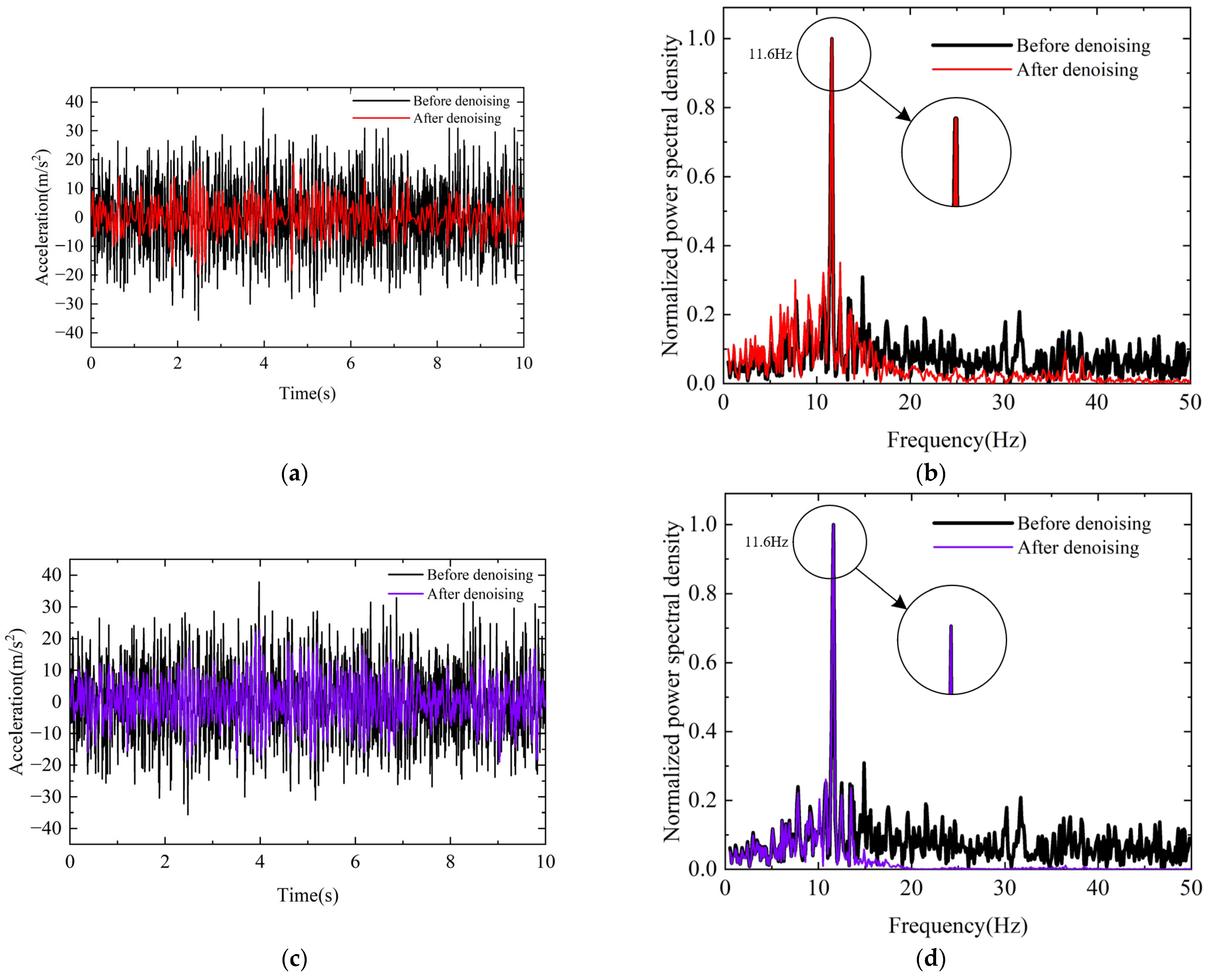
Taking the vertical acceleration at measuring point No. 3 on the main beam of Gate A as an example, the denoising performance of the proposed methods is demonstrated. Figure 8 presents the time–history curves of acceleration before and after denoising, together with the corresponding normalized power spectral density (PSD) comparisons obtained using the EMD-MPE-IWTD and VMD-MPE-IWTD approaches.

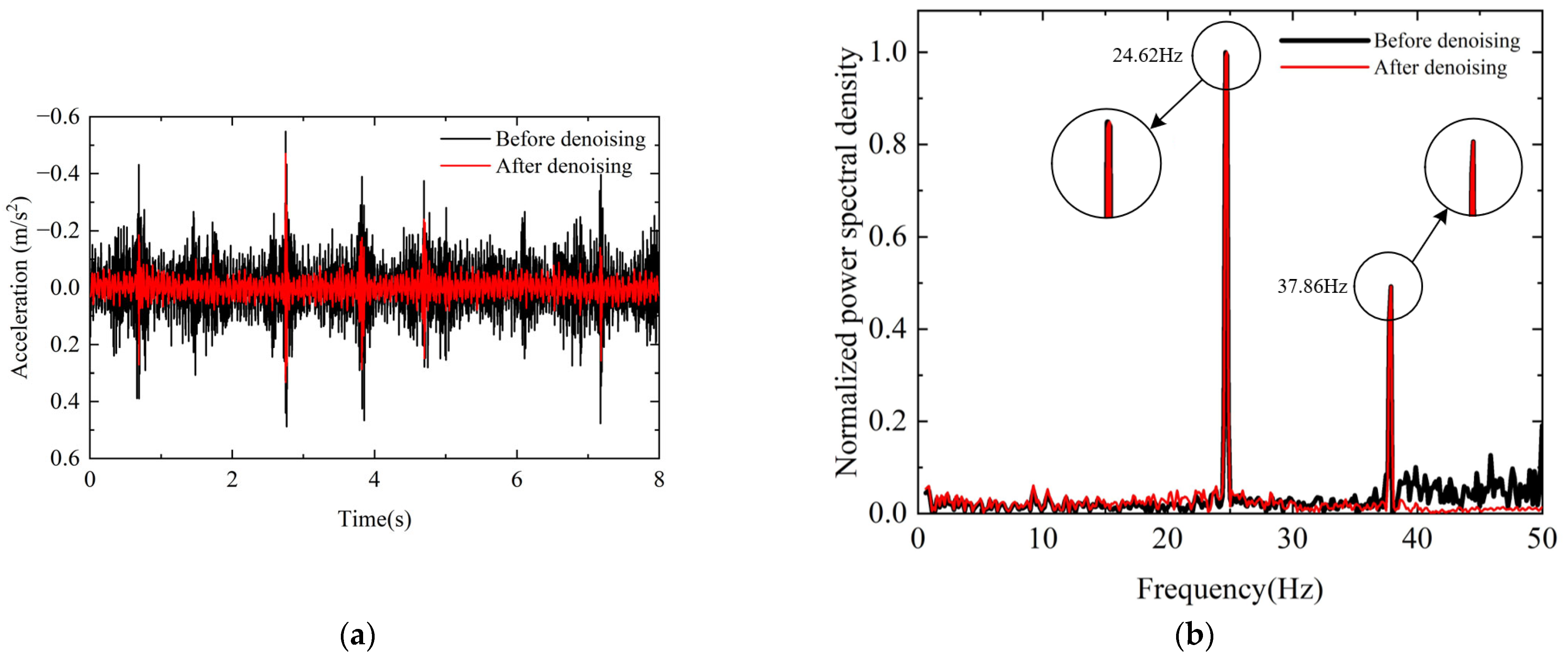
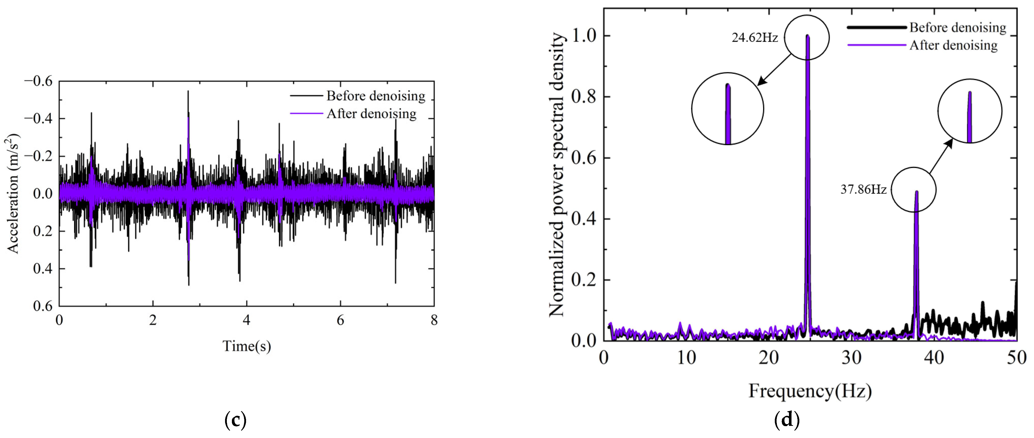
As can be visually observed, both algorithms exhibit evident improvements in time–domain smoothness and high-frequency suppression in the frequency domain. Taking the vertical acceleration at measuring point No. 3 on the supporting arm of Gate B as an example, the denoising performance of the proposed methods is illustrated. Figure 9 presents the acceleration time–history curves before and after denoising, together with the corresponding normalized power spectral density (PSD) comparisons obtained using the EMD-MPE-IWTD and VMD-MPE-IWTD methods.

Based on the comparisons of the pre- and post-denoising time–history curves shown in Figure 8 and Figure 9, it can be observed that the amplitude fluctuations in the signals are significantly reduced after denoising, and the time–domain responses become noticeably smoother.

Further comparison of the normalized power spectral density (PSD) curves before and after denoising reveals that, regardless of the algorithm used, the dominant frequency of the selected signal in Project A remains at 11.6 Hz, while that of Project B remains at 24.62 Hz and 37.86 Hz after denoising. This consistency indicates that the principal energy components are fully preserved without any frequency shift. Meanwhile, the high-frequency components are effectively suppressed, and the spurious spectral energy at high frequencies is substantially attenuated.

To further connect preprocessing with practical monitoring indicators, we quantified the peak-centered band power by integrating the PSD within ±0.5 Hz around the dominant peaks identified from the pre-denoising PSD. As summarized in

Table 4. Peak-centered band-power indicators before and after denoising for field cases (Projects A and B; reference peaks from the pre-denoising PSD; bandwidth: ±0.5 Hz).

Project	Decomposition Method	Fixed Dominant Peak(s) (Hz)	Band (Hz)	Band Power Before	Band Power After	Ratio (After/Before)
A	EMD	11.60	[11.10, 12.10]	0.34033	0.34775	1.0218
	VMD	11.60	[11.10, 12.10]	0.34033	0.34903	1.0256
B	EMD	24.62	[24.12, 25.12]	0.31144	0.31603	1.0147
		37.86	[37.36, 38.36]	0.13973	0.14487	1.0367
	VMD	24.62	[24.12, 25.12]	0.31144	0.31586	1.0142
		37.86	[37.36, 38.36]	0.15503	0.14593	0.94129

, the peak-centered band power remains close to unity for the dominant bands in both Projects A and B under EMD and VMD, indicating that the resonance-related energy used in operational assessment is largely preserved after preprocessing. A modest reduction is observed for the 37.86 Hz band under VMD in Project B, while the dominant peak locations remain unchanged, suggesting that the proposed denoising mainly suppresses broadband interference without shifting the key resonant components.

It should be noted that, in practical engineering tests, the true “clean” signal is typically unavailable, making it impossible to directly evaluate the denoising performance using the conventional signal-to-noise ratio (SNR).

To address this limitation, the denoising noise ratio (dnSNR) is introduced as an evaluation metric to quantify the denoising strength, defined as follows:

$$dnSNR=10\lg (P_s/P_g)$$

(11)

where P_s denotes the average power of the original noise-contaminated signal, which is typically expressed as the mean square value of the signal, i.e.,

$$P_s={\displaystyle \frac{1}{N}}{\displaystyle \sum _{i=1}^N{x}_{raw}^2}(i)$$

(12)

where x_raw(i) represents the original measured signal before denoising, and N is the total number of sampling points. P_g denotes the power of the components removed by the algorithm, which is defined as the mean square power of the difference between the original and denoised signals:

$$P_g={\displaystyle \frac{1}{N}}{\displaystyle \sum _{i=1}^N[x_{raw}}(i)-x_{denoised}(i){]}^2$$

(13)

where x_denoised(i) denotes the signal after denoising.

From a physical perspective, P_g can be interpreted as the energy of the filtered disturbance components—primarily consisting of high-frequency noise, random fluctuations, and other non-structural responses—while P_s represents the total energy of the original measured signal. Accordingly, the dnSNR quantifies the relative magnitude of the removed energy with respect to the original signal energy. A smaller dnSNR indicates that P_g is large relative to P_s, implying that the denoising algorithm has removed a greater portion of the signal energy and achieved stronger noise suppression. Conversely, a larger dnSNR suggests that the removed energy fraction is smaller, indicating a weaker or more conservative noise reduction effect.

The comparison of denoising results for measuring point No. 3 on the surface-bay radial gate of Project A, using the proposed joint denoising method against the conventional WTD and IWTD approaches, is summarized in

Table 5. Comparison of dnSNR results for different algorithms (Project A).

	dnSNR		dnSNR
WTD	20.663	IWTD	2.306
EMD-MPE-WTD	15.239	EMD-MPE-IWTD	1.254
EEMD-MPE-WTD	15.238	EEMD-MPE-IWTD	1.190
CEEMD-MPE-WTD	15.870	CEEMD-MPE-IWTD	1.178
CEEMDAN-MPE-WTD	15.228	CEEMDAN-MPE-IWTD	1.211
ICEEMDAN-MPE-WTD	15.216	ICEEMDAN-MPE-IWTD	1.235
VMD-MPE-WTD	6.427	VMD-MPE-IWTD	1.101

.

The comparison of denoising results for measuring point No. 3 on the deep-bay radial gate of Project B, obtained using the proposed joint denoising method and the conventional WTD and IWTD approaches, is presented in

Table 6. Comparison of dnSNR results for different algorithms (Project B).

	dnSNR		dnSNR
WTD	1.732	IWTD	0.726
EMD-MPE-WTD	1.360	EMD-MPE-IWTD	0.562
EEMD-MPE-WTD	1.449	EEMD-MPE-IWTD	0.651
CEEMD-MPE-WTD	1.469	CEEMD-MPE-IWTD	0.658
CEEMDAN-MPE-WTD	1.285	CEEMDAN-MPE-IWTD	0.551
ICEEMDAN-MPE-WTD	1.355	ICEEMDAN-MPE-IWTD	0.559
VMD-MPE-WTD	1.075	VMD-MPE-IWTD	0.492

.

Based on the dnSNR comparison results from both engineering cases, it can be concluded that, from the perspective of wavelet-threshold denoising, the improved wavelet-threshold denoising method (IWTD) exhibits significantly superior performance compared with the conventional WTD approach. It effectively enhances the signal-to-noise ratio and reduces residual noise components.

From an overall denoising strategy standpoint, decomposition–denoising joint methods (such as EMD-MPE-IWTD and VMD-MPE-IWTD) consistently outperform single-step denoising approaches, thereby validating the effectiveness and rationality of the proposed improved threshold function and the integrated denoising strategy.

5. Joint Denoising Software Development

5.1. Development Framework

To meet the needs of rapid on-site data processing and comparative analysis, an integrated vibration-signal denoising and analysis system was developed on the MATLAB platform (MATLAB R2024a, The MathWorks, Inc., Natick, MA, USA). The system modularizes multiple representative time–frequency analysis and adaptive decomposition algorithms (EMD, EEMD, CEEMD, CEEMDAN, VMD, etc.) and integrates IMF discrimination based on multiscale permutation entropy (MPE), correlation coefficient, kurtosis, and related metrics, together with both classical and improved wavelet-thresholding algorithms.

The system embeds several intelligent optimization algorithms (e.g., particle swarm optimization, PSO; whale optimization algorithm, WOA; sparrow search algorithm, SSA) to automatically tune key hyperparameters in the decomposition and denoising pipeline for superior processing performance. Users may either enable optimization for automatic parameter search or manually specify parameters for finer control. The platform supports a complete workflow—from raw data import, algorithm configuration and execution, parameter optimization, to results review and export—thereby markedly improving the efficiency, stability, and reproducibility of engineering data processing. The architecture adopts a layered design comprising a data layer, an algorithm layer, and a presentation layer.

5.1.1. Data Layer

The data layer handles signal ingestion, preprocessing, and unified management. Field-measured acceleration signals (common formats such as “.mat” and “.txt” are supported) can be imported. The system automatically performs basic preprocessing—DC removal, sampling-rate unification, and analysis-window selection. The preprocessed data are standardized and stored as internal working variables and then passed uniformly to downstream algorithmic modules, enabling normalized data flow and efficient management.

5.1.2. Algorithm Layer

The algorithm layer encapsulates each denoising method at the function level to form interchangeable “processing modules.” Typical modules include the following:

(1)

Decomposition module: Decomposes the input signal to extract a series of intrinsic mode functions (IMFs), characterizing energy distribution and dynamics across frequency bands.

(2)

Discrimination module: Provides customizable criteria (e.g., MPE, kurtosis, correlation coefficient, energy ratio). Users can flexibly choose criteria and thresholds according to signal characteristics. The system adaptively selects components based on indicator values: lower-index components typically correspond to structural principal modes or stable narrowband content, whereas higher-index components are often high-frequency noise or random disturbances.

(3)

Denoising module: Applies targeted suppression, correction, and reconstruction to the selected components. This module supports classical wavelet thresholding and the improved wavelet thresholding proposed herein.

5.1.3. Presentation Layer

The presentation layer serves end users by visualizing and exporting results. The system automatically generates pre-/post-denoising time–history comparisons, normalized power spectral density (PSD) comparisons, and dnSNR-based improvement metrics, thereby intuitively demonstrating time–domain smoothing, dominant-frequency preservation, and high-frequency suppression. All results can be exported with one click for direct inclusion in technical reports or publication figures, greatly enhancing standardization and efficiency of result presentation.

5.2. Results Presentation

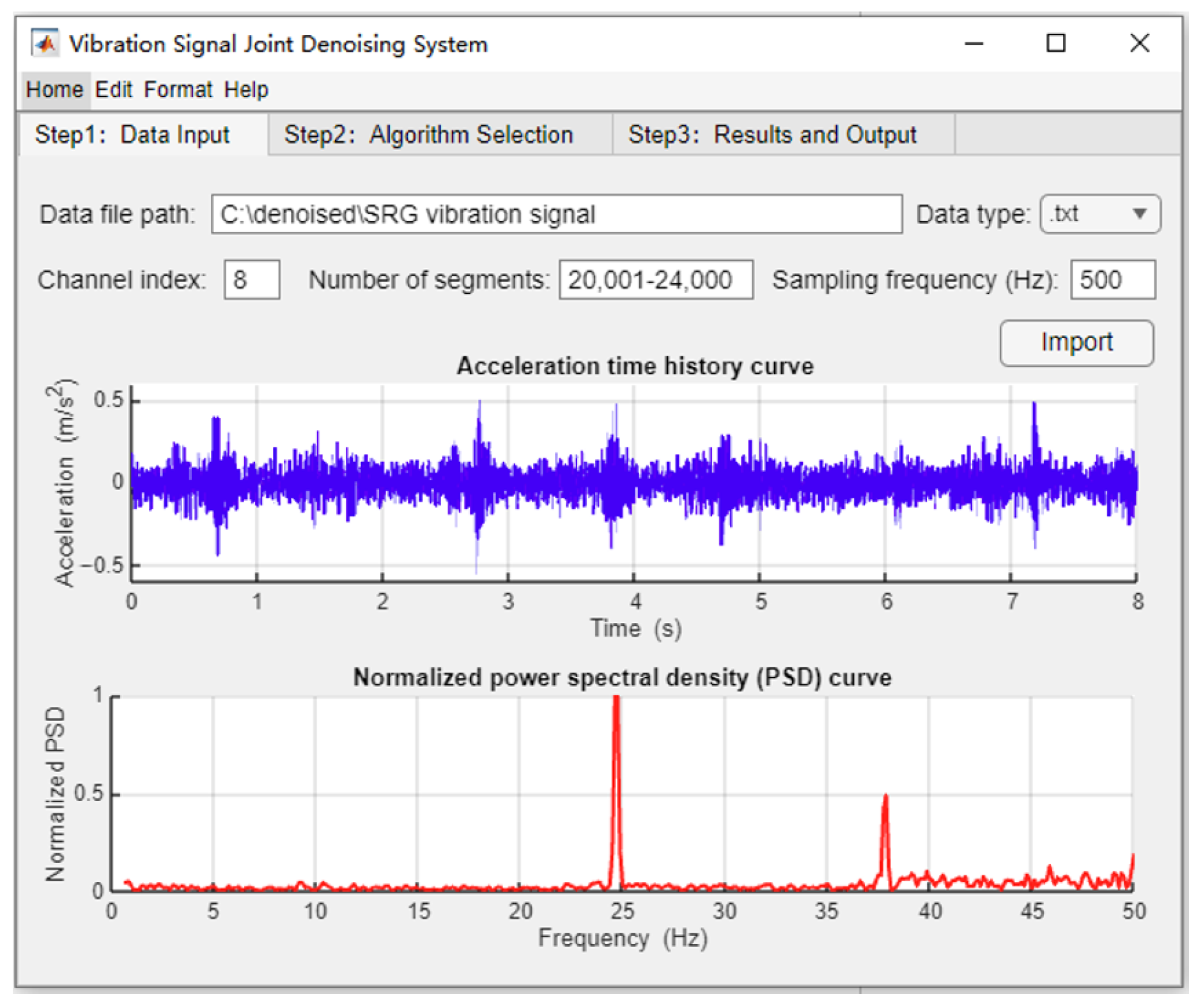
Following the above framework, the system assembles and integrates the algorithm libraries and demonstrates functionality using real engineering data. As an example, the acceleration record at measuring point No. 3 in Project B is used as input, with the data file path set to “C:\denoised\SRG vibration signal”. In the data-input interface, the data type is set to “.txt”, channel index to 8, the row range to 20,001–24,000, and the sampling frequency to 500 Hz. After clicking “Import,” the system automatically reads the file and displays the acceleration time–history and the corresponding normalized PSD for the selected channel. The data input module interface is shown in Figure 10.

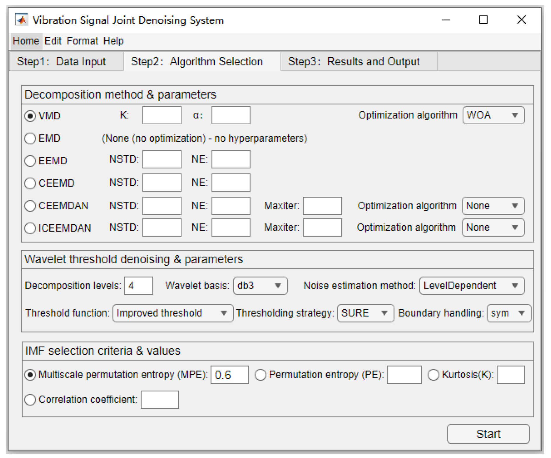
Next, the algorithm selection module is entered, which consists of three functional panels: decomposition algorithms, denoising algorithms, and IMF discrimination algorithms.

In the decomposition panel, the system provides multiple options including VMD, EMD, EEMD, CEEMD, CEEMDAN, and ICEEMDAN, with reserved interfaces for optimization algorithms. When the optimization function is enabled, the system’s built-in intelligent optimization algorithms can automatically search for optimal hyperparameters. When disabled, users may manually specify the relevant parameters through the input fields.

The denoising panel is designed based on the wavelet-thresholding theory, allowing users to customize the decomposition level, wavelet basis, and thresholding function type (soft-, hard-, or improved-threshold function proposed in this study) to accommodate different signal characteristics.

The IMF discrimination panel offers several selectable criteria, including multiscale permutation entropy (MPE), permutation entropy, kurtosis, and correlation coefficient. Users can choose the desired metric and specify the threshold value to achieve adaptive identification and selection of components.

In the functional demonstration, the selected configuration was as follows: the decomposition algorithm was VMD, the optimization algorithm was WOA, the wavelet decomposition level was set to 4, the wavelet basis was db3, and the threshold function adopted the improved wavelet threshold proposed herein. The IMF discrimination criterion was based on MPE, with a threshold value of 0.6. The interface of the algorithm selection module is shown in Figure 11.

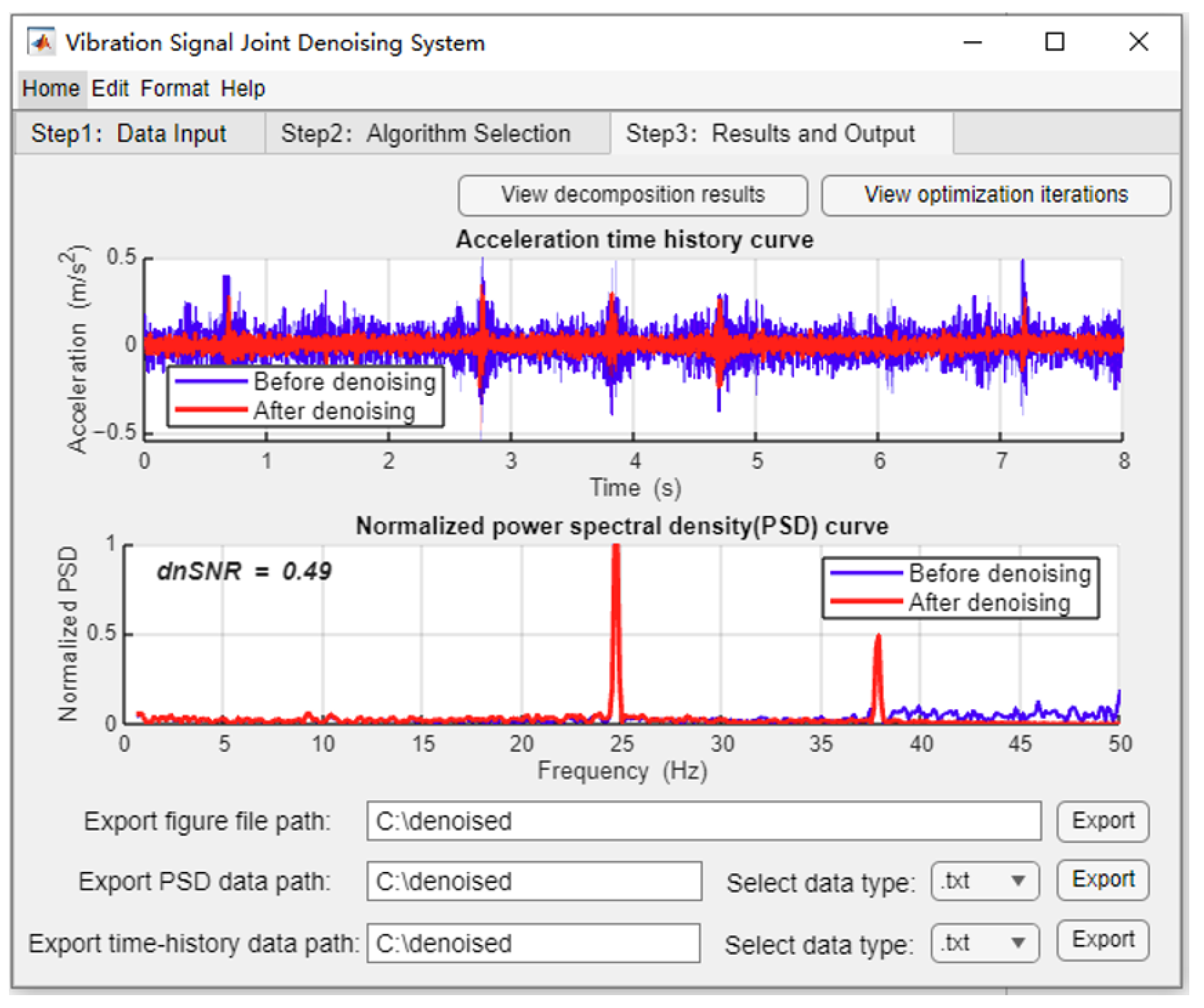
Finally, the results visualization and output module presents the comparative outcomes of the denoising process, including the time–history curves and normalized power spectral density (PSD) curves. It also automatically computes the improvement in signal-to-noise ratio (dnSNR), enabling users to quantitatively assess the denoising performance.

The module provides interactive viewing capabilities: by clicking the “View decomposition results” button in the upper-right corner, users can inspect the detailed decomposition results of the signal; when optimization algorithms are enabled, clicking the “View optimization iterations” button allows users to visualize the iterative convergence process of the optimization procedure.

Finally, users can specify the output directory and file format to export the time–history and normalized PSD data in “.txt”, “.csv”, or “.mat” formats for further analysis and reporting. The interface of the results visualization and output module is shown in Figure 12.

6. Conclusions

This study proposes a decomposition–denoising-based vibration-signal denoising framework and develops an application-oriented denoising system for radial steel gates under discharge excitation.

(1)

A smooth and tunable thresholding strategy is introduced to enable controlled filtering in wavelet-based denoising, reducing threshold-induced artifacts and improving the preservation of diagnostically relevant structural characteristics in non-stationary vibration signals.

(2)

An integrated “decomposition–selection–selective denoising–reconstruction” workflow is established, where multiscale permutation entropy is used to identify noise-dominated components and only these components are denoised prior to reconstruction. This coupled strategy treats noise suppression as a coherent process rather than a single-step operation, enhancing robustness under strong interference conditions.

(3)

The proposed framework is validated using benchmark signals with a known reference and two field-measured engineering cases of radial steel gates. The results show clearer time histories and more stable dominant spectral characteristics after preprocessing. In addition, the developed system encapsulates decomposition, denoising, and parameter-selection modules into a user-oriented workflow, facilitating practical deployment for engineering signal preprocessing and subsequent vibration-based condition assessment.

Future work will extend the evaluation to multiple noise realizations. It will also investigate downstream diagnostic tasks such as modal identification and feature stability assessment.