Article

Modeling Methodology of Paper Craft Aerial Acrobatic Robot Using Multibody Dynamics

by
Kazunori Shinohara
1,* and
Kenji Nishibori
1,2
1
Department of Mechanical Systems Engineering, Daido University, 10-3 Takiharu-cho, Minami-ku, Nagoya 457-8530, Japan
2
Nagoya Industrial Science Research Institute, Nagoya Chamber of Commerce & Industry Building, 2-10-19 Sakae, Naka-ku, Nagoya 460-0008, Japan
*
Author to whom correspondence should be addressed.
Appl. Sci. 2026, 16(2), 921; https://doi.org/10.3390/app16020921
Submission received: 15 December 2025 / Revised: 5 January 2026 / Accepted: 8 January 2026 / Published: 16 January 2026
(This article belongs to the Section Robotics and Automation)

Abstract

The aerial acrobat robot is a mechanical structure that achieves continuous acrobatic motion without electrical power by utilizing gravitational potential energy.The power of this motion is the rotational motion resulting from the imbalance of moments caused by both the masses, called counterbalance, and the weight of the robot. Or, it is the rotational motion resulting from the reciprocal energy conversion between the gravitational potential and kinetic energy of these two masses. Using the quasi-static single-link model mechanism, we derived a formula for the power moment that is important in the design of the mechanical structure to produce the aerial acrobat robot’s motion. This structure is mainly made of resin and is approximately 2 m long. Based on this structure, we developed a paper craft aerial acrobat robot compacted to about 0.27 m so that anyone can easily play with it. In the paper craft aerial acrobat robot based on the quasi-static single-link model, instability in the rotational behavior becomes apparent. To enhance the accuracy of the analysis of rotational moments, which are crucial in design, we develop a modeling method for a paper craft aerial acrobat robot using multibody dynamics. Furthermore, the theoretical solution for a simplified model of the paper craft aerial acrobat robot is constructed based on the double pendulum. The dynamic moments obtained by the modeling method of the paper craft aerial acrobat robot is verified by comparing the theoretical solution.

1. Introduction

The entertainment robot market is rapidly growing and is expected to reach USD 41.0 billion by 2025 and USD 89.4 billion by 2028. However, research on robots has primarily focused on practical applications, leaving entertainment uses largely unexplored. Entertainment plays a crucial role as a foundation for building human–robot relationships. Entertainment robots have the potential to enhance human experiences and strengthen user relationships through emotional engagement [1,2]. From an engineering perspective, entertainment robots often involve distinctive dynamic characteristics, such as lightweight structures, large-amplitude rotational motion, and the effective use of mechanical energy without complex actuation systems. These characteristics are not limited to entertainment purposes but are also closely related to fundamental challenges in the study of space robots and industrial robots, where lightweight design, energy efficiency, and dynamic motion play essential roles [3,4,5]. In particular, the dynamic behavior of swinging and rotational motion under limited energy input shares similarities with motion problems encountered in space robotics, such as tethered systems, deployable structures, and free-floating manipulators [6]. Among such systems, the aerial acrobat robot (also referred to as a trapeze robot) serves as a representative example. This robot operates using only mechanical potential energy without electrical power and continuously climbs along an inclined line through repeated swinging motion. Research on the aerial acrobat robot was initiated in 2008 by Nishibori et al. [7,8].
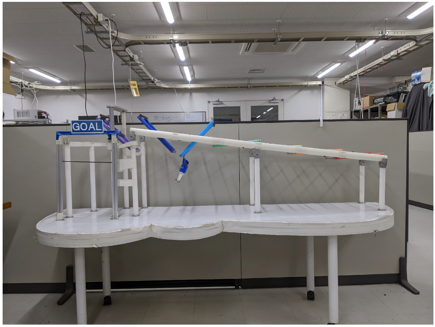
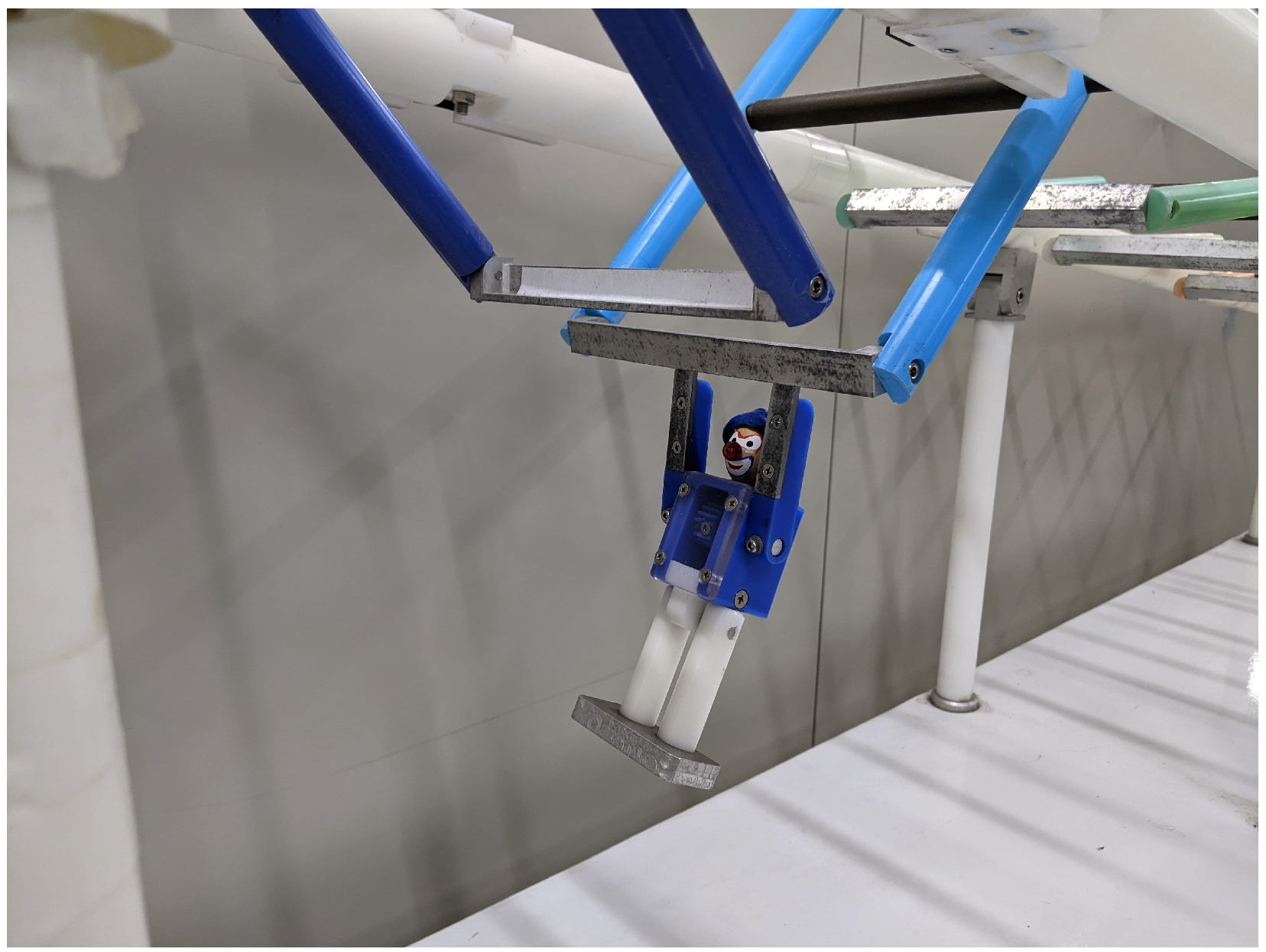
The research behind the aerial acrobat robot is inspired by several previous studies of robots performing various acrobatic acts. There are three prior studies referenced. A method was proposed to control the motion of a horizontal bar robot by utilizing resonance phenomena to excite swinging and employing the entrainment phenomenon of nonlinear oscillators to synchronize and control the first and second links [9]. The dynamic characteristics of a brachiation-type mobile robot are mathematically modeled and analyzed, and optimal control methods for its movement are examined. Brachiation is a mode of locomotion used by monkeys, in which they hang from tree branches and move using their arms. This motion involves gripping a branch with one arm, swinging the body like a pendulum, and reaching for the next branch to progress forward [10,11,12]. An aerial acrobat robot was developed, inspired by the movements of a tightrope-walking automaton, one of the traditional karakuri puppets believed to have been created in the Owari (today, Nagoya) region during the Edo period. This robot utilizes the phenomenon of swing oscillation for aerial mobility, with research conducted on its mechanism and control methods. The tightrope walking karakuri puppet features a “karako” doll (a doll depicting a child with Chinese style hair and clothing engaged in play) suspended from evenly spaced horizontal bars. A puppeteer manipulates strings attached to the doll, causing it to perform front flips and move forward along the bars in a unique and captivating manner [13,14]. Nishibori et al., inspired by Japan’s traditional karakuri [15], noted the lack of research at the time on systems capable of continuously moving along horizontal bars or swings without relying on electrical power [7]. They embarked on the development of an aerial acrobat robot that utilizes mechanical energy to traverse a series of swings successively. This innovative approach aimed to replicate the motion of traditional karakuri, which often relied on clever mechanical designs rather than modern electrical systems. By focusing on mechanical energy, the team sought to create a robot capable of moving through a sequence of swings in a manner reminiscent of historical automata [16,17,18]. As shown in Figure 1 and Figure 2, early research in 2008 led to the development of a structure enabling the robot to traverse a series of upward-sloping swings. Based on the moments calculated through quasi-static analysis for the swing frame [7], a structural design was developed. This structure is fabricated primarily using resin materials. However, the handrails of the swing frame are made of aluminum, and the counterbalance is made of brass. As for the robot, the head and legs are made of wood and resin, while the torso, the arms, and feet are made of aluminum. This design enabled the aerial acrobat robot to achieve stable traversal motion.
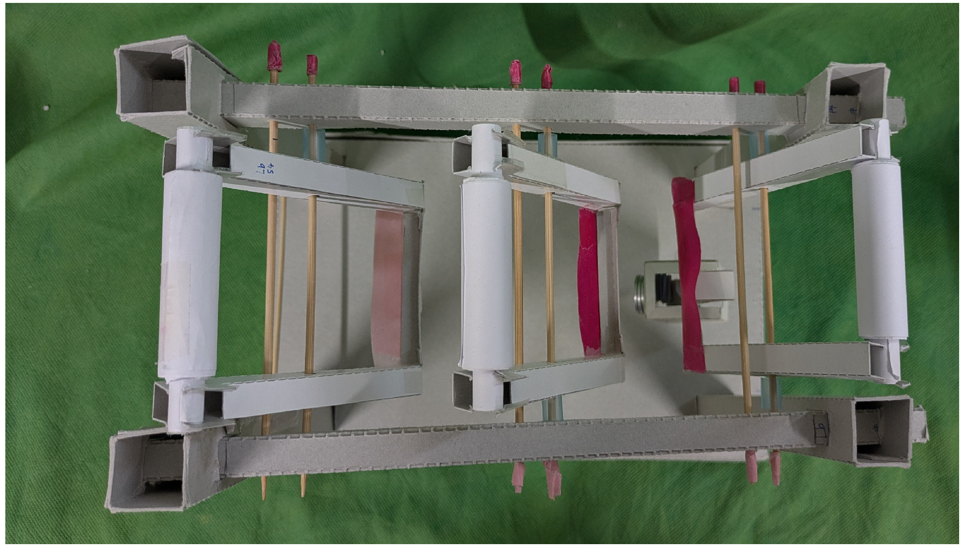
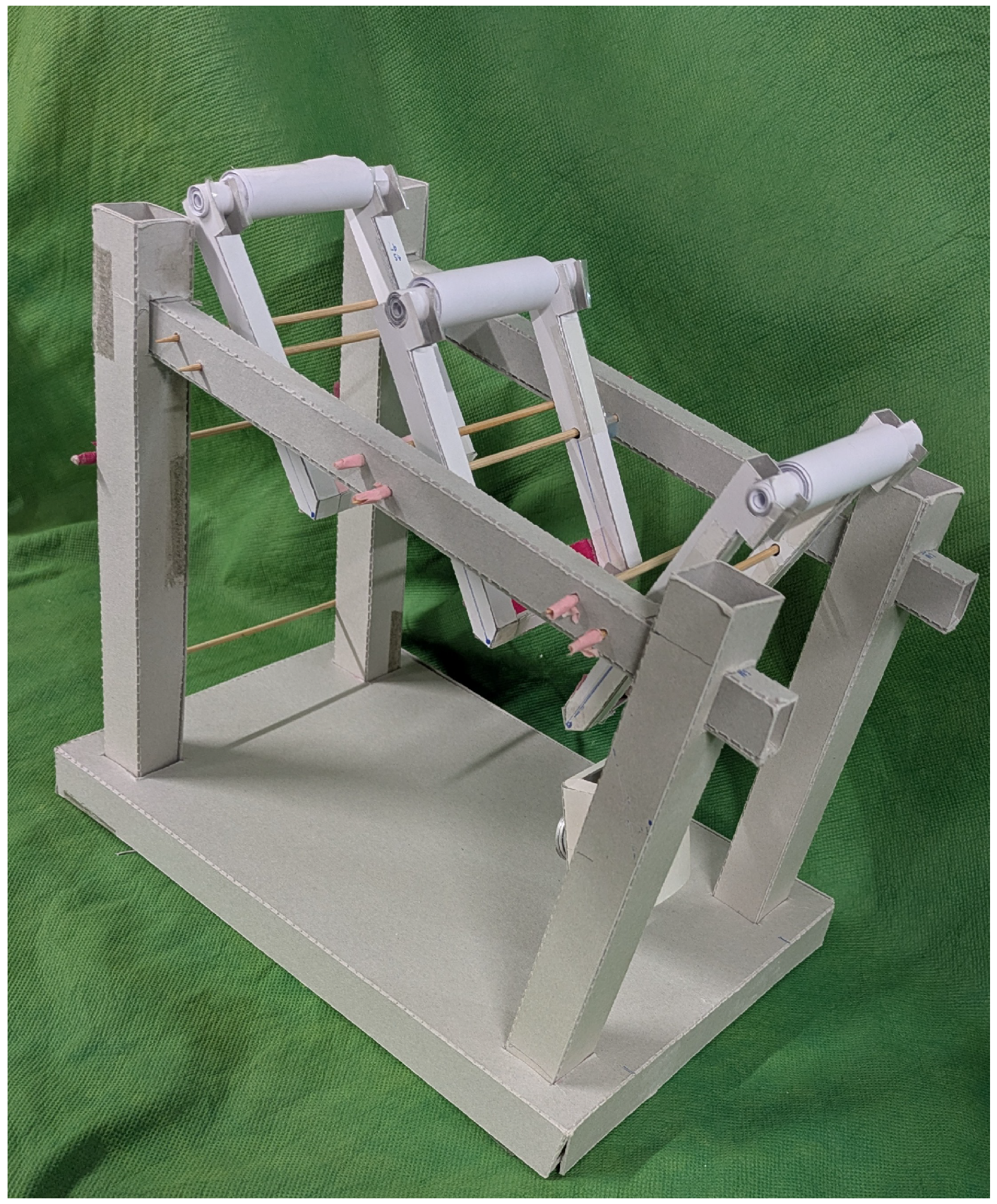
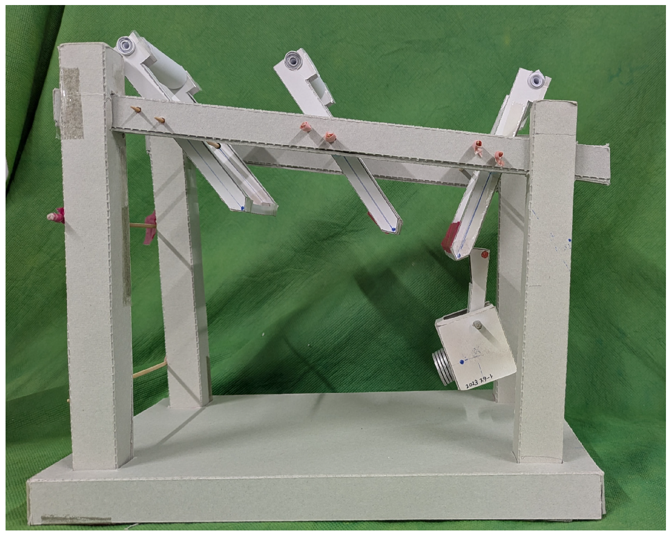
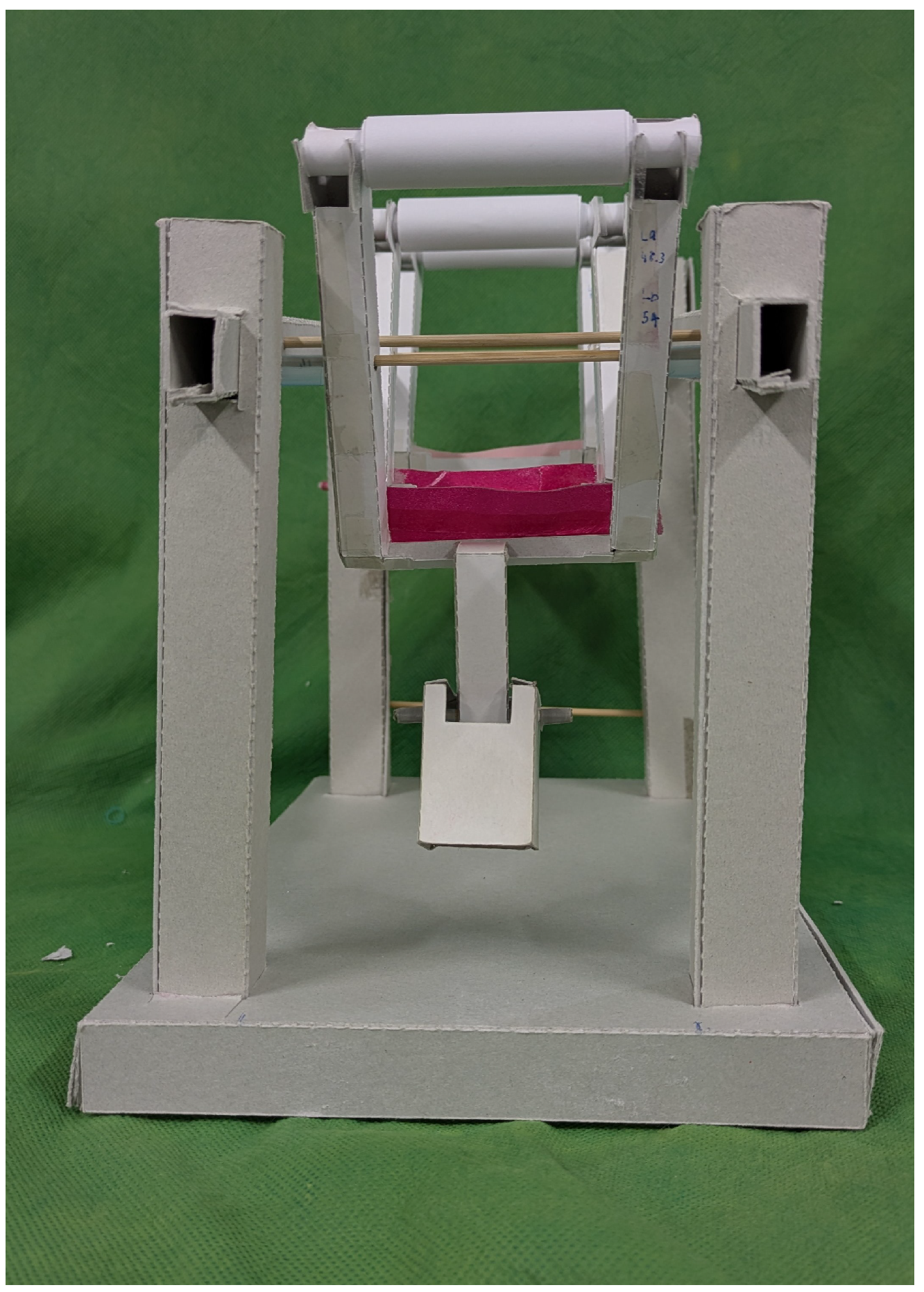
The structure of this large aerial acrobat robot posed challenges, as its high production cost and size made it inaccessible for casual use by everyone. To address these limitations, efforts are directed toward reducing the mass and size of the aerial acrobat robot, leading to the development of a compact, paper-based version as shown in Figure 3, Figure 4, Figure 5 and Figure 6. To make the aerial acrobat robot more accessible and enjoyable, a smaller, paper-craft version is created using paper and bamboo skewers, downsizing the original large design. By utilizing paper, advantages such as easily obtainable materials and reduced production time are achieved. On the other hand, when creating the small paper craft aerial acrobat robot based on the quasi-static theoretical moments of the swing frame, the failure rate of the robot’s tightrope traversal significantly increased. By suspending a counterbalance on one end of the swing frame and the robot on the other end, a slight mass imbalance generates rotational moment in the swing frame. A crucial aspect of the aerial acrobat robot’s design is the conversion of gravitational energy into rotational energy, ensuring that a continuous rotational moment is consistently produced in one direction. Furthermore, the success of the robot’s traversal from one swing frame to the next depends on whether this rotational moment is effectively generated and maintained during the transition. To determine this rotational moment precisely, a theoretical framework based on dynamics incorporating angular velocity and angular acceleration would be necessary. However, since data on the swing frame’s angular velocity and angular acceleration cannot be obtained during the preliminary design stage, such theoretical formulas are impractical for this purpose. Nishibori et al. developed a theoretical formula based on quasi-static approximation that allows for simple inference before the design stage. This formula estimates the threshold using data on the frame dimensions, mass, position, and moment of inertia of the aerial acrobat robot. In such theoretical formulas, the design based on Nishibori’s theory posed no significant issues for a large aerial acrobat robot, even with slight variations. However, in the case of a small paper-based model, there are instances where the swing frame failed to generate rotational momentum in one direction.
The limitations of the conventional design evaluation method proposed by Nishibori, which calculates the rotational moment of the swing frame, have become apparent. Designing based on this evaluation method, such as determining key dimensions or masses, can hinder the robot’s motion. Therefore, the aim of this study is to improve the accuracy of calculating the rotational moment of the swing frame—an essential energy source—through a modeling approach using multibody dynamics analysis. As will be discussed later, it is found that the time variation in the rotational moment differs between Nishibori’s conventional evaluation method and the evaluation method based on multibody dynamics. To evaluate which method better represents the rotational moment of the swing frame, a comparative analysis is conducted using measured the rotational moment data obtained from image-based measurements of actual motion, along with a double-pendulum model governed by the Lagrangian equations of motion and multibody dynamics. Through this comparison, the effectiveness of Nishibori’s conventional evaluation method and that of the multibody dynamics approach in representing the actual rotational moment is examined.

2. Structure of Paper Craft Aerial Acrobat Robot

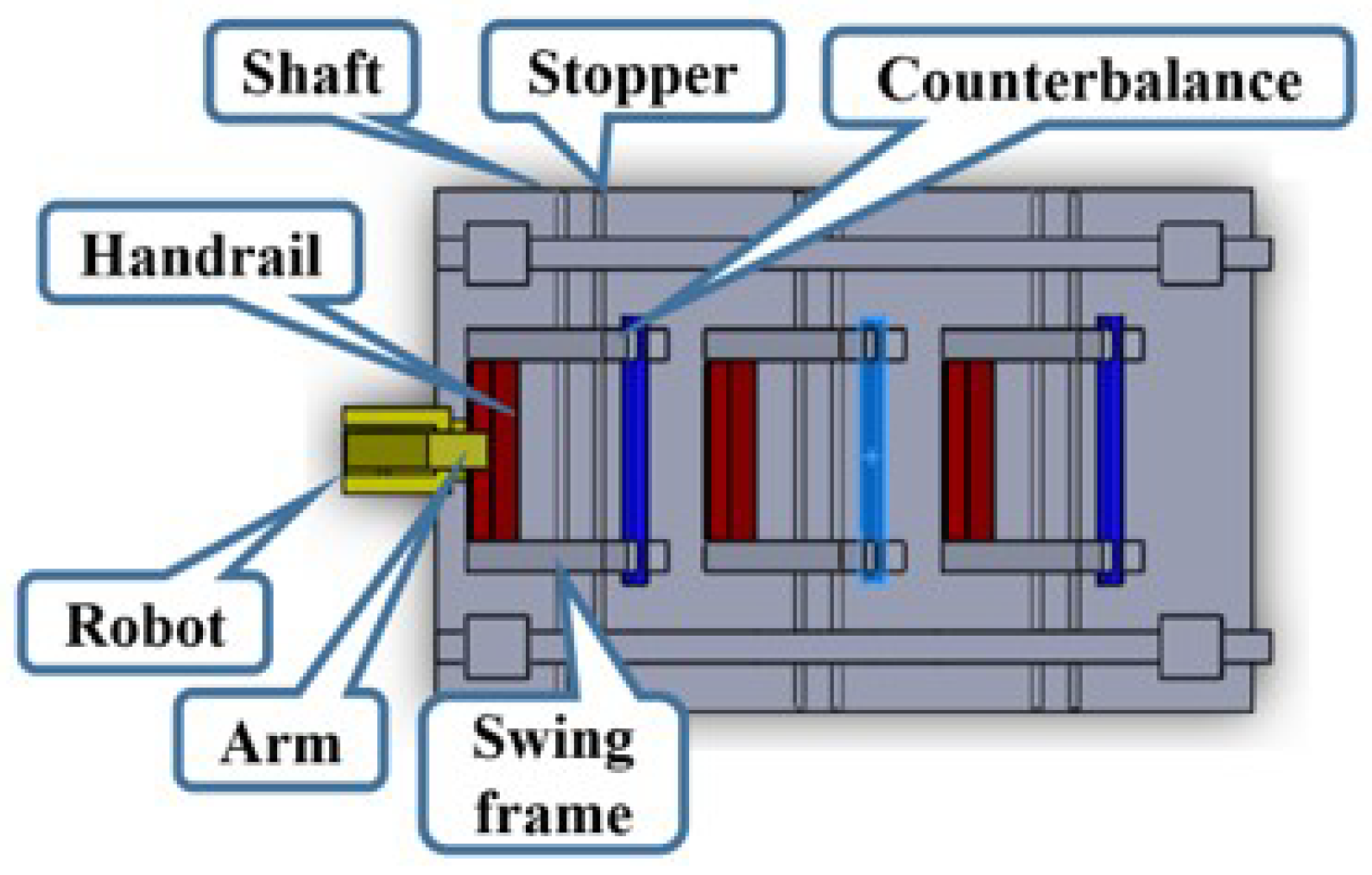
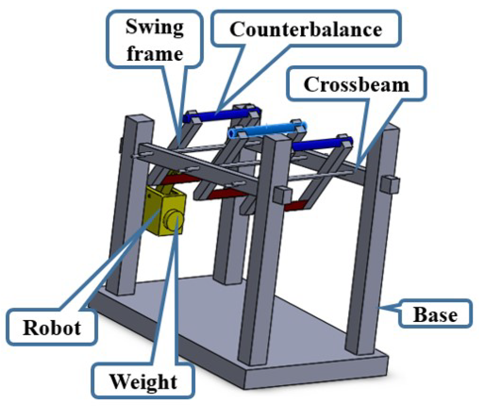
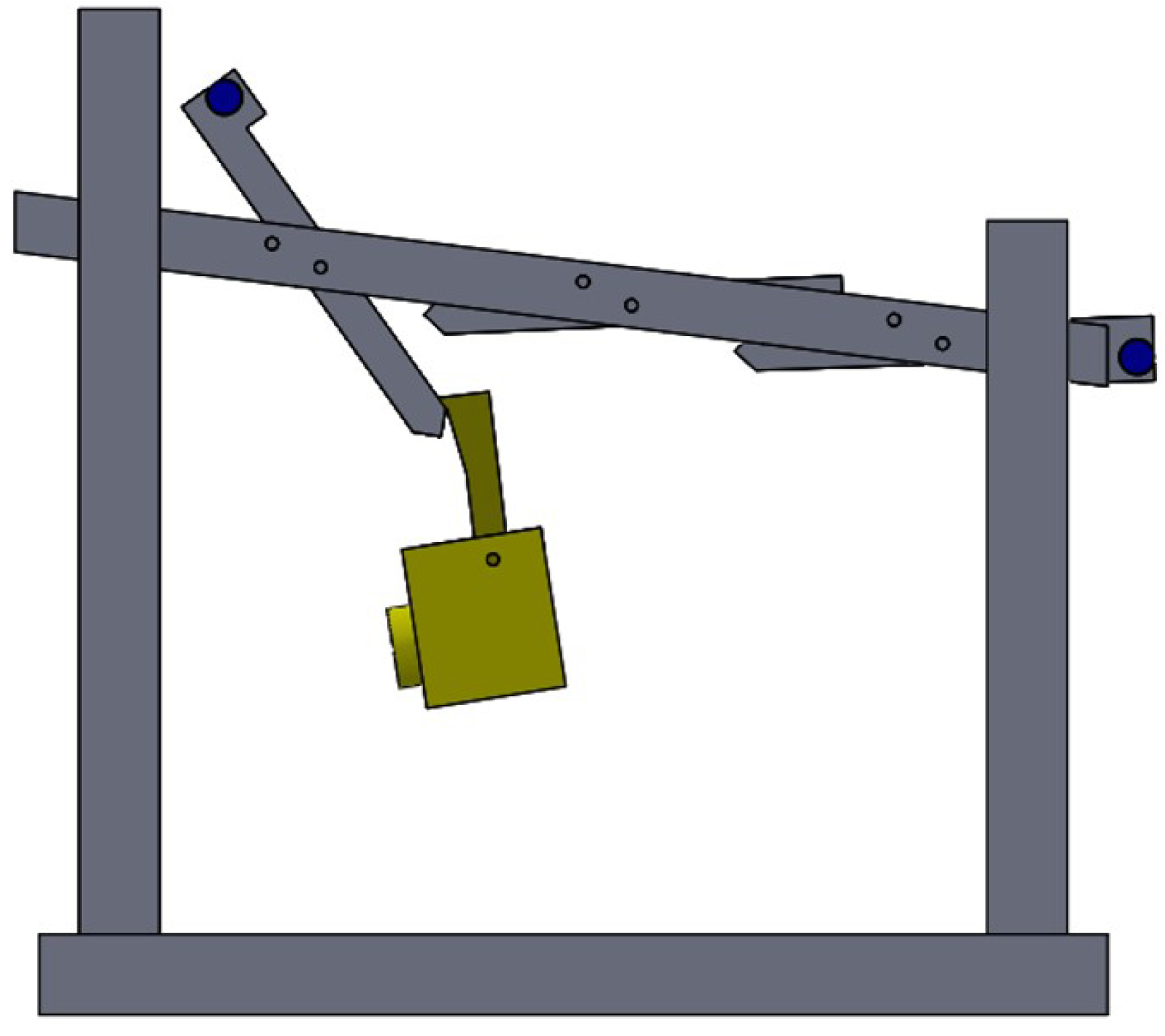
As shown in Figure 7 and Figure 8, the structure of the paper craft aerial acrobat robot can be broadly divided into three components: the base, the swing frame, and the robot. The base consists of multiple beams and crossbeams that are necessary for fixing the swing frames and forming multiple rows of them. The two crossbeams that fix the row of swing frames are angled relative to the plane of reference. This angle represents the incline that allows the robot to gradually ascend against gravity. Two bamboo skewers are placed between two crossbeams: one serves as the rotation axis for the swing frame, and the other functions as a stopper to halt its rotation. These skewers are referred to as the rotation axis and the rotation stopper, respectively. Using these axes, the robot is transported from the left end to the right end, where its movement is stopped. The swing frame has a hollow rectangular shape, with a handrail at one end for suspending the robot and a counterbalance at the other end. The counterbalance consists of a concentrated mass.
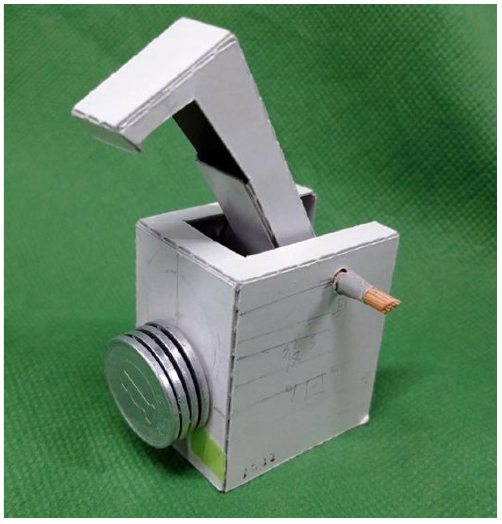
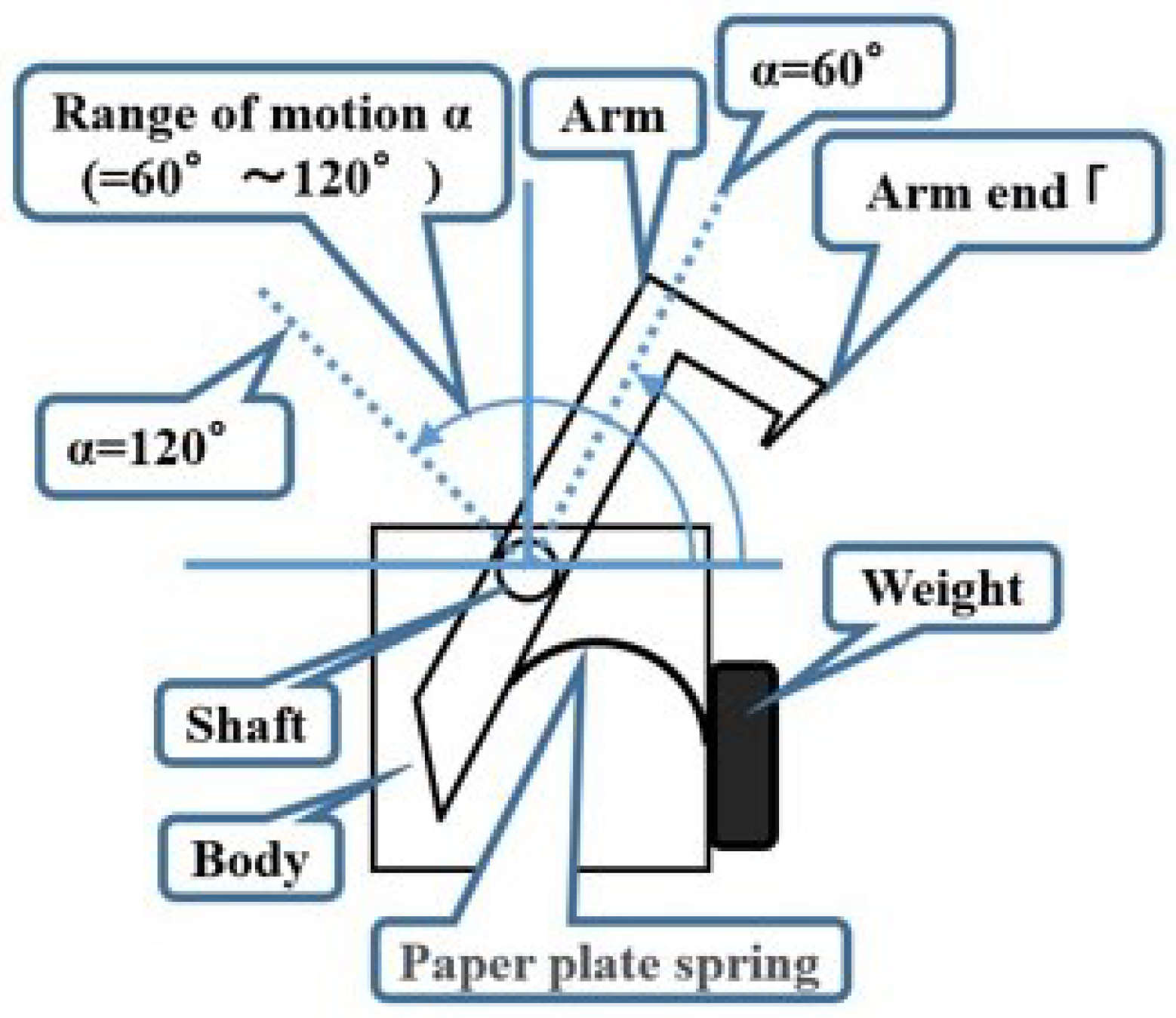
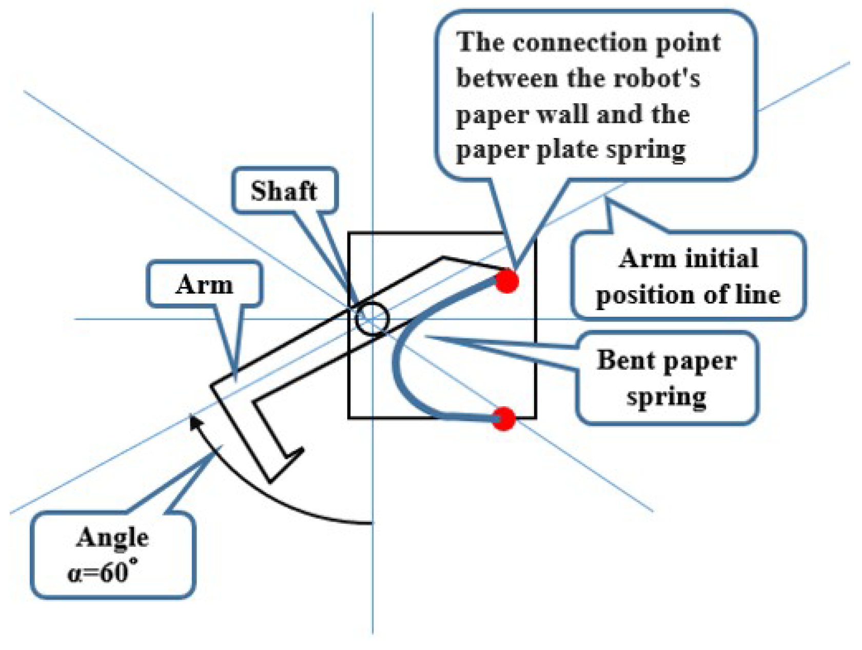
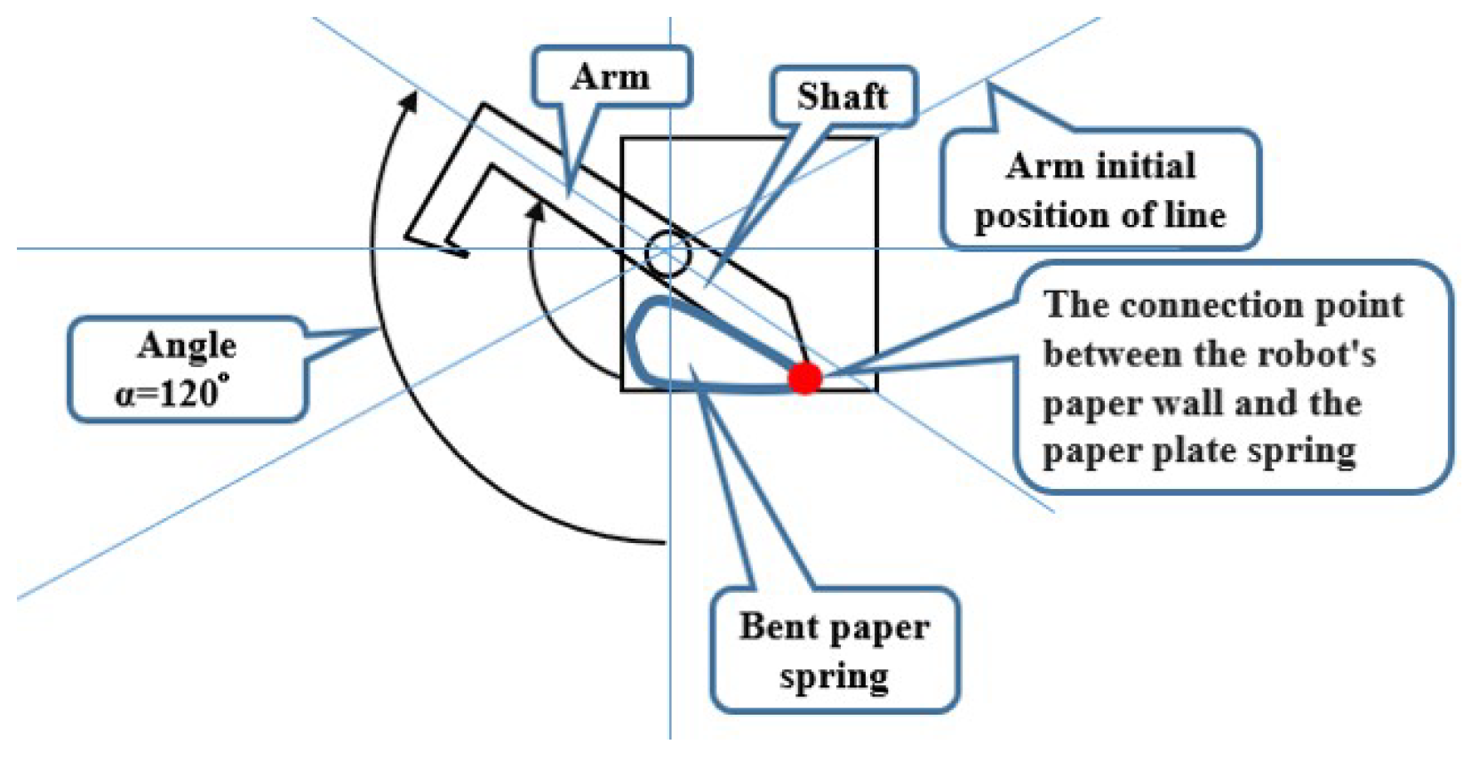
Figure 9 and Figure 10 show the robot. The robot consists of a torso, an arm, a paper leaf spring, and a weight. In the conventional large-scale aerial acrobat robot, the robot had two arms. However, in the paper craft aerial acrobatic robot presented in this study, the number of arms is reduced to one in order to simplify the structure and enable low-cost, easy assembly. A paper leaf spring is attached between the torso and the arm. The torso is equipped with an axle, allowing the arm to rotate around the torso. The angle  α  of the arm has a movable range of approximately  60  to  120 . When the arm and the handrail are fixed, the robot hangs below the handrail, and the paper leaf spring bends due to the influence of the robot’s weight. At this point, the angle  α  of the arm is approximately  120 . When the arm detaches from the handrail, the bent paper spring attempts to return to its straight form. The restoring force of the flexed paper spring causes the robot’s arm to snap forward, protruding ahead of its torso. At this stage, the angle  α  of the arm is approximately  60 .

3. Motion of Paper Craft Aerial Acrobat Robot Model

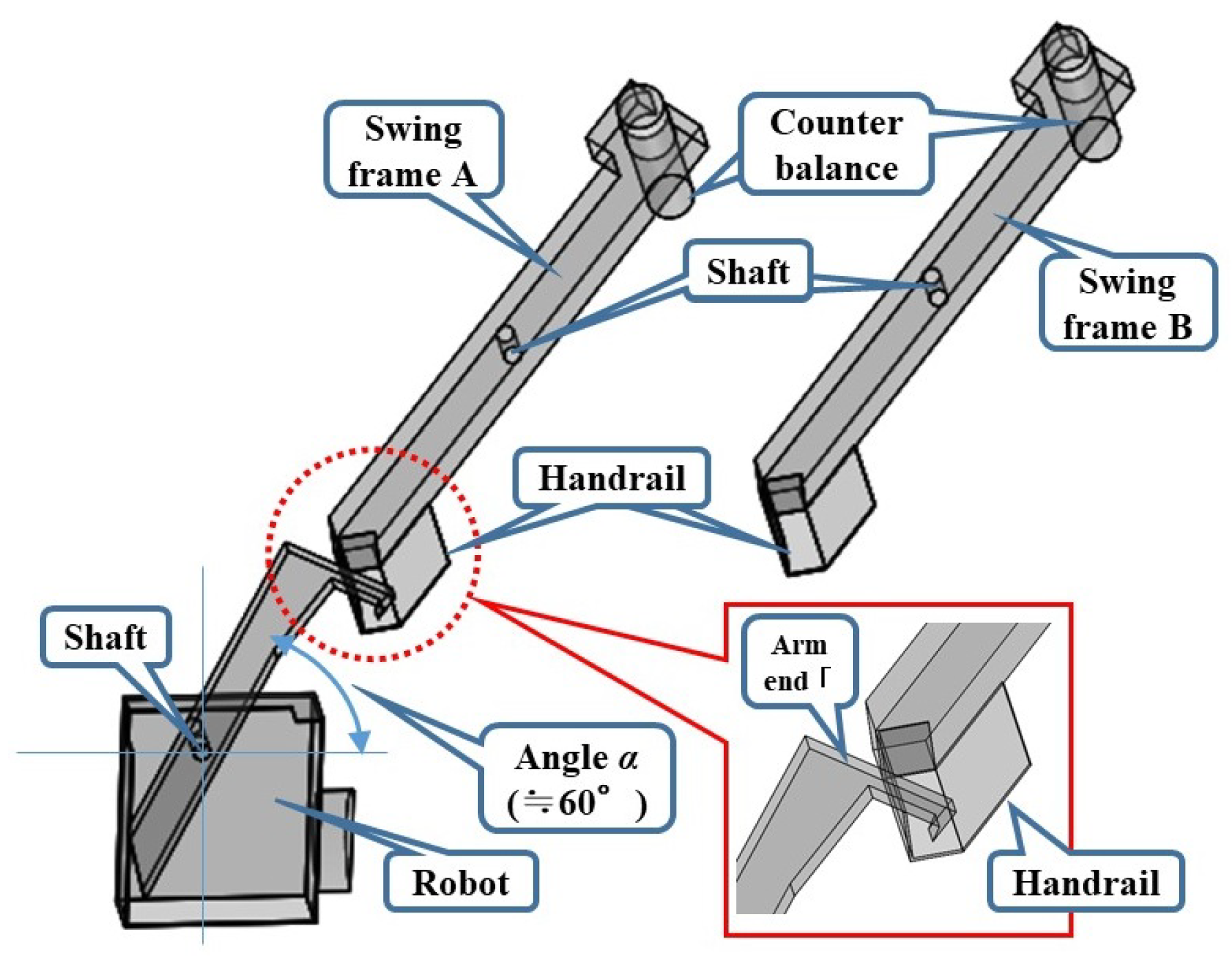
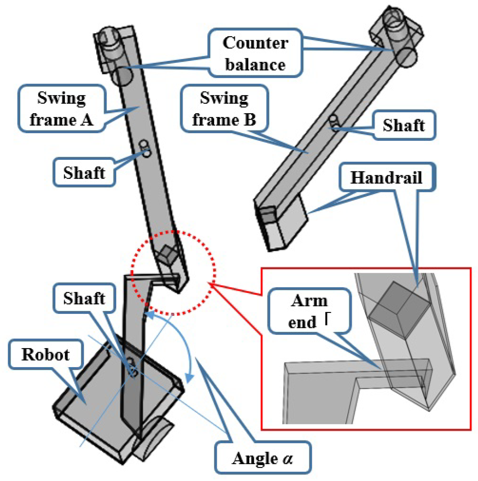
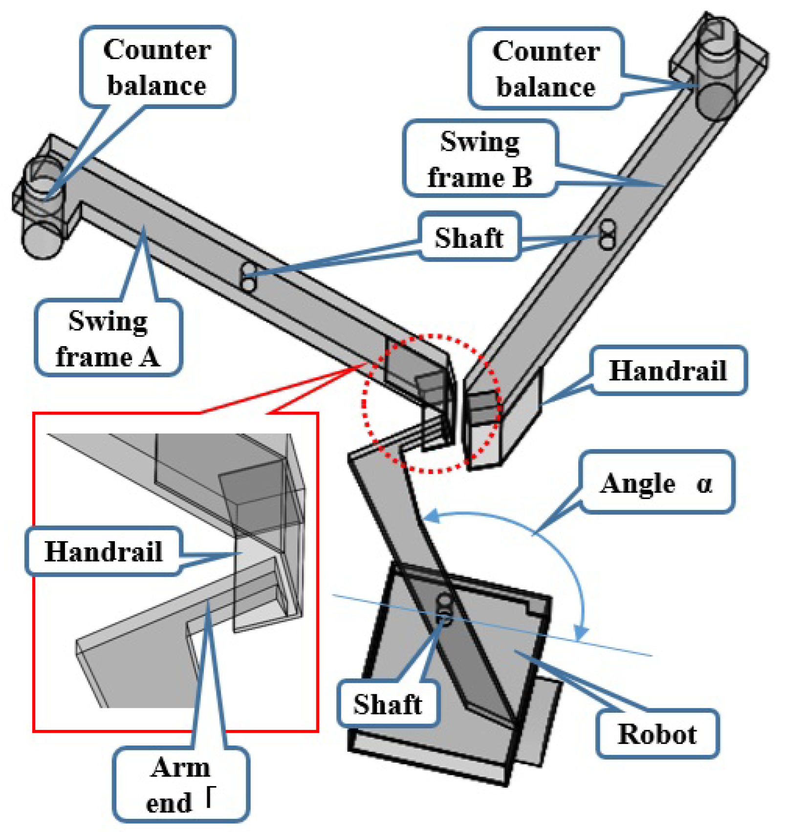
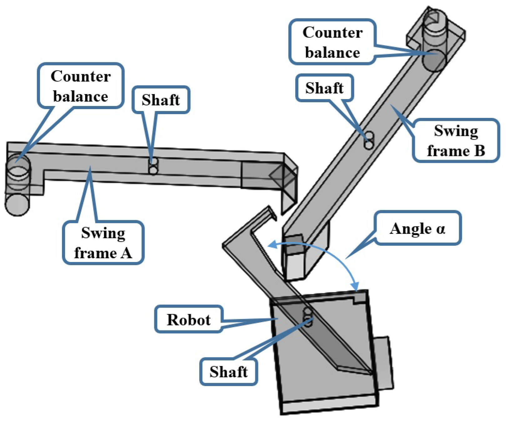
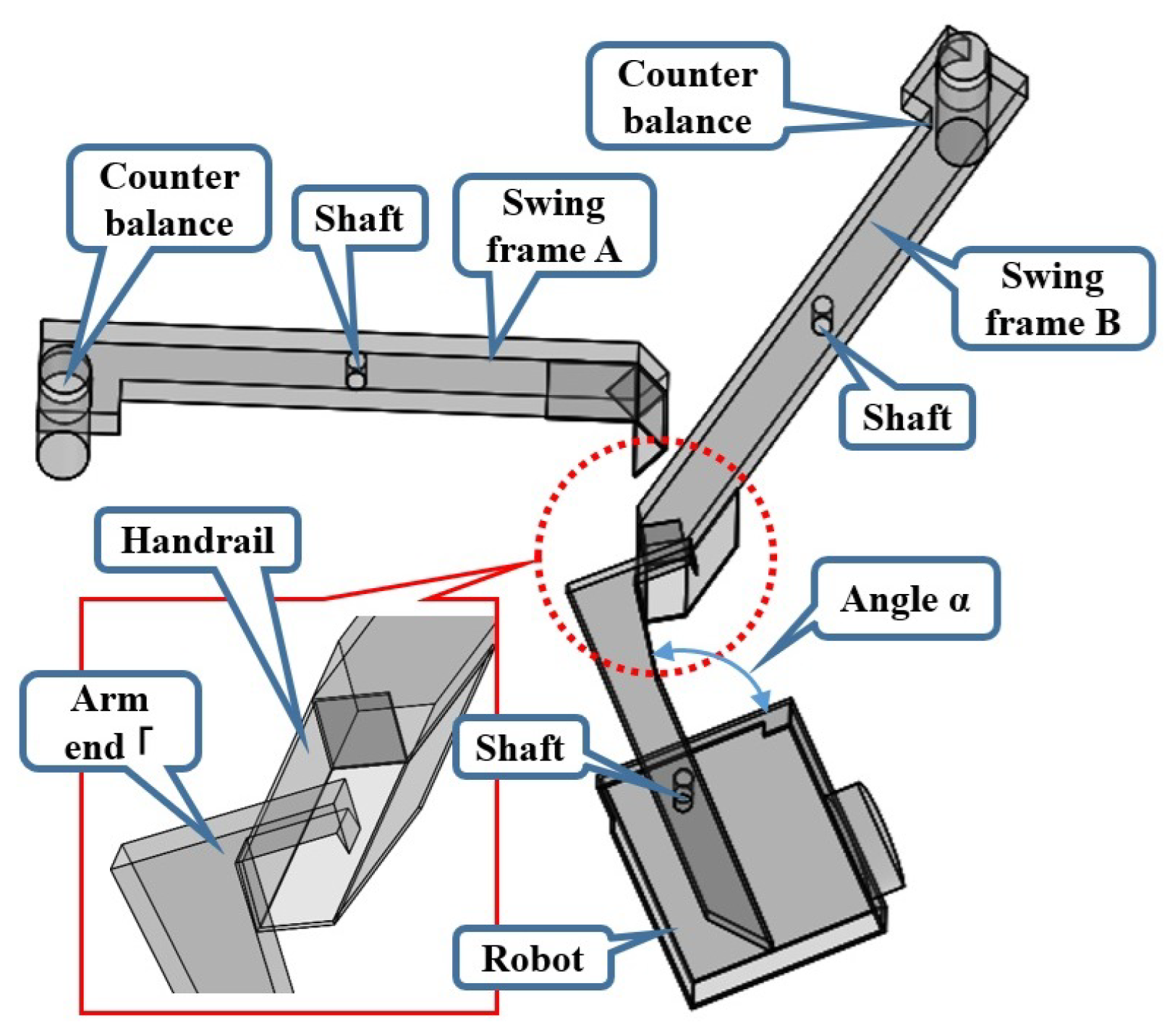
Figure 11, Figure 12, Figure 13, Figure 14 and Figure 15 show an extracted diagram of the entire structure, focusing on the swing frame A and the adjacent swing frame B. The swing frame A represents the state in which the robot is hanging. Both the tip of the arm and the handrail have an L-shaped design, allowing the arm tip (⌜-shaped) and the handrail (⌟-shaped) to come into contact with each other. The contact between the arm and the handrail is maintained by both the friction force and the normal force, which act as reaction forces generated by the robot’s weight. At one end of the swing frame A, the robot’s weight is suspended by the arm on the handrail, while the other end has a counterbalance. Since the mass of the robot is greater than the mass of the counterbalance, the imbalance in their masses generates a rotational moment in swing frame A. As the potential energy of the mass of the robot decreases, it is converted into the robot’s kinetic energy and the rotational energy of the swing frame A. Figure 12 shows the state where the robot is at its lowest position, and the counterbalance is at its highest position. The counterbalance has the maximum potential energy. Additionally, as shown in Figure 21, the paper leaf spring is at its maximum deflection, and the arm angle  α  reaches its maximum value of  120 . As the swing frame rotates, the L-shaped contact surface tilts, reducing the normal force, as shown in Figure 13. This reduction also causes the frictional force to be reduced. As illustrated in Figure 14, during the transition, the robot’s arm slips off the handrail due to gravity. Subsequently, since the robot has detached from the swing frame A, the swing frame A continues to rotate as the potential energy of the counterbalance is converted into rotational kinetic energy until it hits the stopper. Finally, the swing frame A collides with the rotation stopper, halting its rotational motion. At this moment, the robot temporarily floats in midair, becoming completely unconstrained from any support as shown in Figure 14. On the other hand, the swing frame B remains stationary due to the gravitational effect of the counterbalance. After the robot’s arm slips off the handrail of the swing frame A, as the bent paper spring tries to return to its original flat shape, it generates a restoring force that acts on the tip of the arm and pushes it forward beyond the torso. As shown in Figure 15, when the robot’s arm ⌜-shaped tip catches onto the adjacent swing Frame B of the ⌟-shaped handrail, the two shapes come into contact with each other, securing the robot once again on the adjacent swing frame B. The adjacent swing frame B then begins to rotate. This sequence of actions is repeated between the robot and the series of swing frames.

4. Theory of Rotational Forces with Respect to the Swing Frame

4.1. Rotational Force Derived from Quasi-Static Using Potential Energy (Conventional Theory)

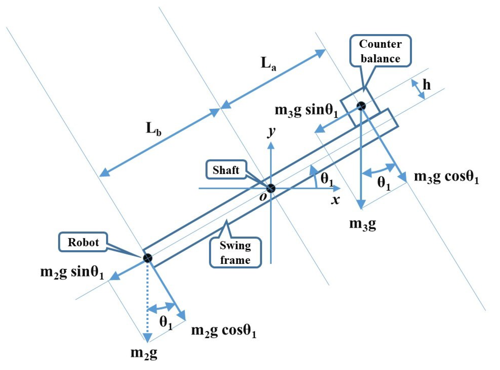
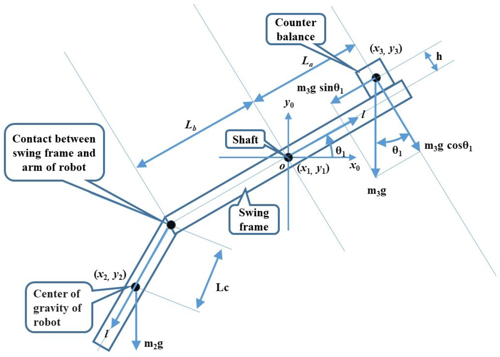
Nishibori et al. developed a formula to calculate the rotational moment of the swing frame based on design dimensions to construct the design of the aerial acrobat robot [7,8]. Figure 16 shows the conceptual diagram of the swing frame based on the one-link model. The axis parallel to the gravity vector is defined as y, and the axis perpendicular to it is defined as x. Figure 16 also illustrates a schematic diagram when the frame is tilted by an angle  θ 1  relative to the x-axis. Nishibori et al. derived the rotational moment formula as follows.
I θ 1 ¨ = m 2 g L b + Δ T cos θ 1 m 3 g L a cos θ 1 + m 3 g h sin θ 1
The variable I represents the total moment of inertia, which is the sum of the swing frame’s moment of inertia  I 1 , the robot’s moment of inertia  I 2 , and the counterbalance’s moment of inertia  I 3 , as shown in the following equation (see the Appendix A for details).
I = I 1 + I 2 + I 3
The variable  θ 1 ¨  represents the angular acceleration of the swing frame, the variable  m 2  denotes the mass of the robot, and the variable  m 3  denotes the mass of the counterbalance. the variable  Δ T  represents the initial moment at  θ 1 = 0  after removing the counterbalance and the robot from the swing frame. The variable  I θ 1 ¨  represents the rotational moment, which serves as the power source for the aerial acrobat robot.
Table 1 summarizes the representative lengths and masses of the robot used in Figure 16 and Figure 17. The mass  m 2  represents the total mass of the following components: the torso mass 0.002 kg, four coins mass 0.004 kg attached to the torso, the arm mass 0.0015 kg, and the handrail of the swing frame mass 0.0021 kg. Due to design constraints on the distance from the swing frame’s axis of rotation to its tip, there is a tendency to use a mass for the robot that is heavier than the counterbalance in order to increase the moment imbalance.

4.2. Rotational Force Derived from Dynamics Using Kinetic and Potential Energy

As will be discussed later, there is a discrepancy between the rotational moment of the swing frame calculated using multibody dynamics and that derived from Equation (1).
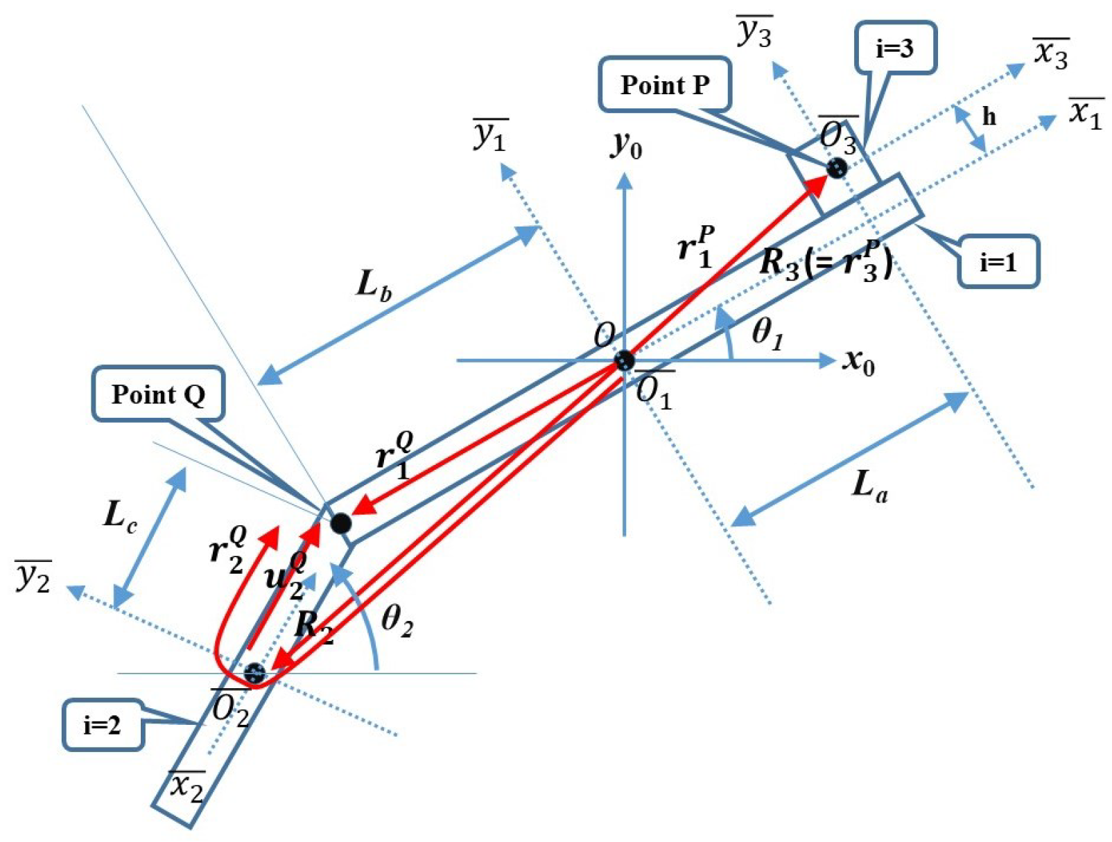
To explain the cause of this discrepancy, the theoretical framework presented in this section is necessary. Figure 17 shows the conceptual diagram of the two-link model used to determine the rotational moment through dynamics based on kinetic and potential energy. The two links shown in Figure 17 represent the swing frame and the robot.  L C  denotes the distance from the contact point between the handrail and the arm, to the center of the robot. By treating the contact point between the robot’s arm and the handrail as a joint between links, the swing frame and the robot are modeled as a double pendulum.
The first link represents the swing frame, which rotates around the fixed support, while the second link represents the robot body, which undergoes rotational motion relative to the frame. This modeling approach is based on the observation that the overall motion is primarily governed by large-amplitude planar rotational dynamics. Degrees of freedom that are not essential to this dominant behavior, such as out-of-plane motion, are excluded from the analytical model. The link structures are assumed to be rigid bodies, and elastic deformation is not considered. Although the aerial acrobat robot is constructed from paper materials, any deformation occurring during motion is sufficiently small relative to the overall rotational displacement. The stiffness of the paper structure is therefore regarded as adequate, allowing the system to be reasonably approximated as a rigid-body mechanism. Although this point is discussed later, the validity of this modeling assumption is also supported by the fact that the time histories of angular acceleration obtained from the numerical analysis and the theoretical model exhibit similar trends.
This model incorporates the influence of the inertial force due to the angular acceleration of the robot’s center of mass, which is neglected in Equation (1), on the rotational moment of the swing frame. The rotational moment of the swing frame shown in Figure 17 is derived. For details on the derivation, the Lagrangian equations of motion and the kinematic analysis method for multibody systems are summarized in Appendix A and Appendix B. Here, conditions are set as follows.
L c = 0
Then,  η 1  to  η 3  are given as follows:
η 1 = I
η 2 = 0
η 3 = m 2 g L b cos θ 1 + m 3 g L a cos θ 1 m 3 g h sin θ 1
Equation (A25), with Equations (3)–(6) substituted, is found to be identical to the equation of motion derived from quasi-static single-link model using potential energy of Equation (1).

5. Measurement of Torsional Spring Constant of Robot

The rotational spring constant of the leaf spring is a critical factor for the robot to successfully perform tightrope walking. The angle  α , which represents the movable range of the arm, is shown in Figure 10. This range approximately spans from  60  to  120 . To successfully perform tightrope walking, it is necessary for the robot’s arm to quickly shift its position from behind the torso ( α = 120 ) to in front of the torso ( α = 60 ) at the moment it slips off the handrail. The component that enables this motion is the paper-based leaf spring. When the arm is in contact with the handrail,  α  is around  120 , and when the arm detaches from the handrail, the influence of the paper spring causes  α  to shift to around  60 . When the arm slips off the handrail, the robot momentarily falls through the air. Below, the handrail of the next row of swing frames is positioned directly underneath, waiting for the robot. If the torsional spring constant of the leaf spring is too low, the arm fails to rotate quickly enough toward the front of the torso to catch the handrail. As a result, the arm misses the handrail, and the robot falls to the ground. On the other hand, if the torsional spring constant of the leaf spring is too high, the arm maintains a posture of  α = 60  even while in contact with the handrail. As a result, when the arm slips off the handrail, it is already at the minimum value of its movable range ( α = 60 ) and does not perform any rotational movement. Consequently, during the robot’s fall, the arm does not move toward the handrail positioned below, and the robot falls to the ground without catching it.
Both the fabrication of the actual robot and the multibody dynamics modeling require an appropriate torsional spring constant to successfully perform tightrope walking. Since the spring is made of paper, the spring constant is extremely small. Commercial spring scales are generally designed to measure forces of 1 N or greater. Because the paper spring exhibits forces on the order of 0.01 N to 0.1 N, measuring the torsional spring constant of the paper leaf spring with a commercial spring scale is not effective.
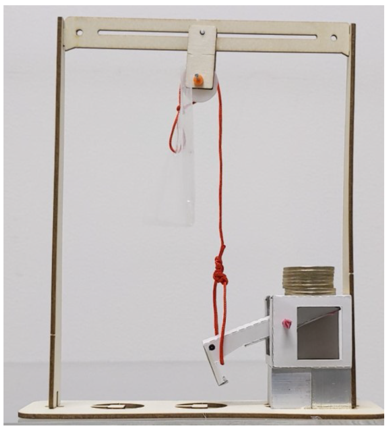
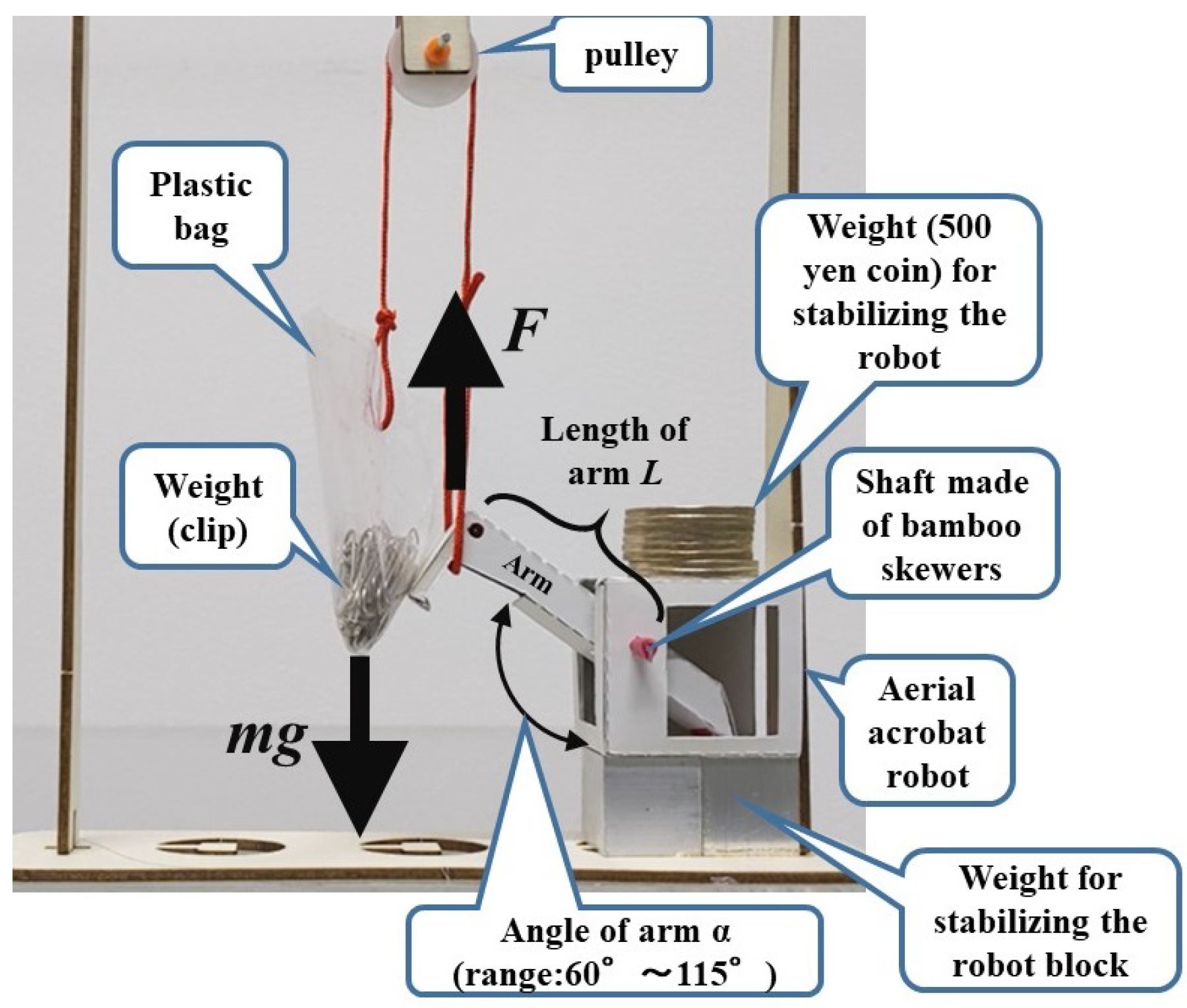
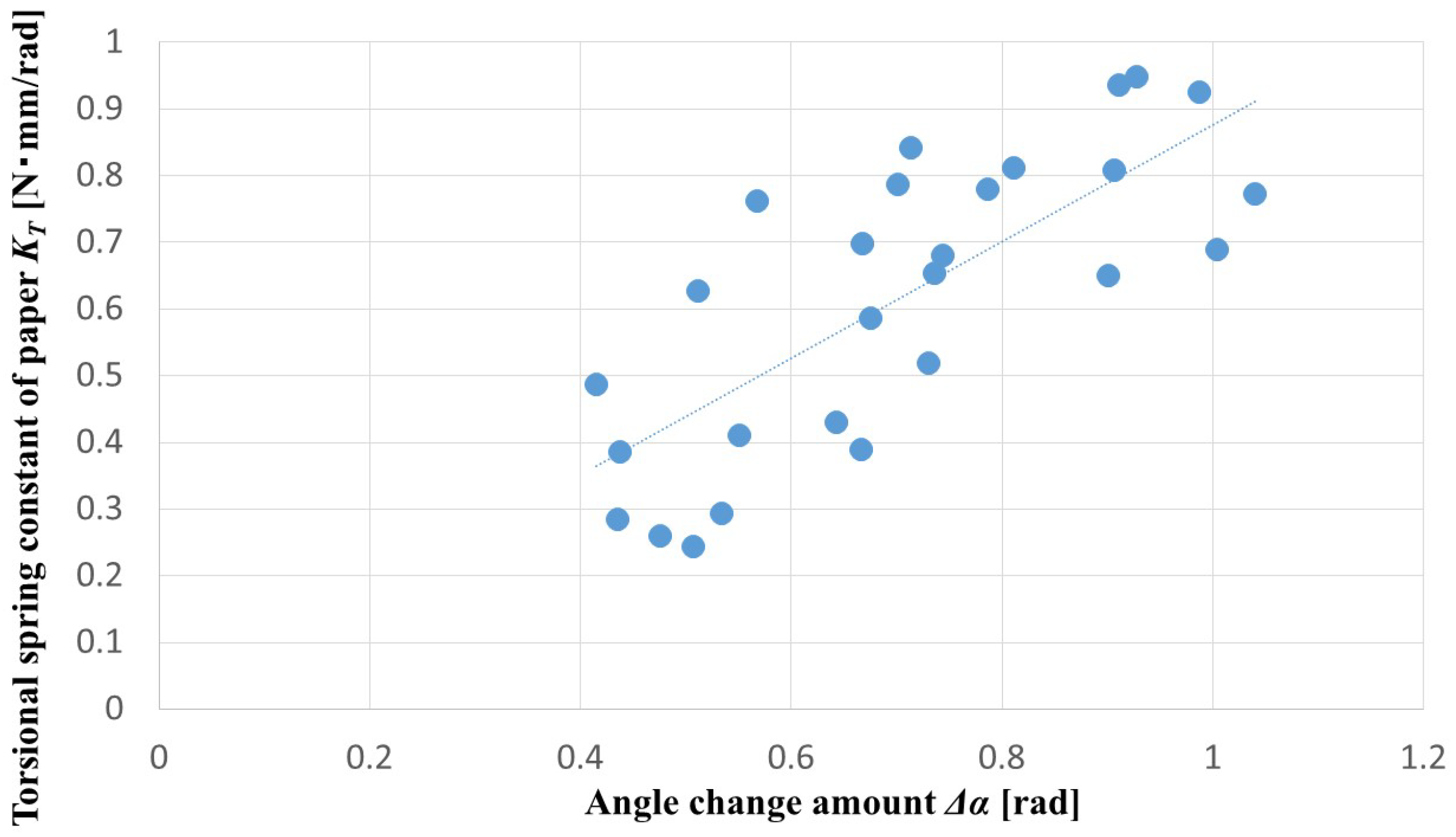
This paper proposes a method for evaluating the leaf spring using a pulley system. Figure 18 shows the setup used to measure the torsional spring constant of the robot’s arm. A pulley is installed at the top, and a rope is passed through it. One end of the rope is attached to the tip of the robot’s arm, while the other end is connected to a plastic bag intended to hold masses. The plastic bag itself has a mass of approximately 0.3 g. The angle change amount  Δ α  of the arm is extracted from the images using Kinovea [20]. In the initial state, the arm angle is  α = 60 . A side view of the robot and the condition of the paper-based leaf spring at that time are shown in Figure 19. From this state, a clip (approximately 0.25 g) is added one by one into the plastic bag. As a result of the increasing mass, the arm moves downward under the influence of the paper-based leaf spring. As shown in Figure 20, the arm angle  α  gradually increases and eventually reaches the maximum value of its movable range  α = 120 . A side view of the robot and the condition of the paper spring at that time are shown in Figure 21. The relationship between the angle change amount  Δ α  and the torsional spring constant  K T  is given by the following equation.
K T = 0.877 Δ α
The above equation represents an approximate straight line obtained from the measured data points as shown in Figure 22 K T  is measured in  N · m m / r a d . The zero point of the horizontal axis, which represents the change in angle  Δ α , corresponds to the initial arm angle  α = 60 . SolidWorks Motion 2019 is used for the multibody dynamics analysis. Since this software requires the torsional spring constant to be defined as a linear function, the approximation curve based on the measured data is also derived as a linear function.

6. Measurement of the Coefficient of Friction at the Contact Surface Between the Swing Frame Handrail and the Robot Arm

As shown in Figure 11, at the moment when the robot’s arm catches on the handrail of the swing frame, the gravitational vector is perpendicular to the vector of the handrail’s inclination. In other words, the arm will not slip off the handrail. However, as the swing frame rotates, as shown in Figure 13, the handrail’s inclination changes, and the gravitational vector gradually becomes more parallel to the inclination vector of the handrail.
As a result, the arm begins to slip along the handrail. If the coefficient of friction is low, slipping occurs before the robot is lifted to a sufficient height by the rotation of the swing frame. Consequently, the arm slips off the current handrail before reaching the handrail of the next swing frame, causing the robot to fall.
On the other hand, if the coefficient of friction is high, the swing frame reaches the stopper, the rotation ends, and the robot moves to a sufficiently high position. However, due to the high friction, sufficient slipping does not occur, and the arm does not detach from the handrail. As a result, the reverse rotation of the swing frame begins under the influence of the robot’s mass, and the resulting translational inertial effect of the robot is reduced. Because the resulting translational inertial effect is small, the robot as a whole does not move in the translational direction. As a result, the robot’s arm fails to catch on the handrail of the adjacent swing frame, leading to the robot’s fall. Therefore, setting an appropriate coefficient of friction is essential for both the development of the paper craft aerial acrobat robot model prototype and the analysis using multibody dynamics.
Although previous studies have measured the coefficient of friction of paper, it has been shown that the value depends on the paper type [21,22]. Therefore, in this study, the coefficient of friction is measured for the specific paper used, following the Japanese Industrial Standards (JIS) [23].
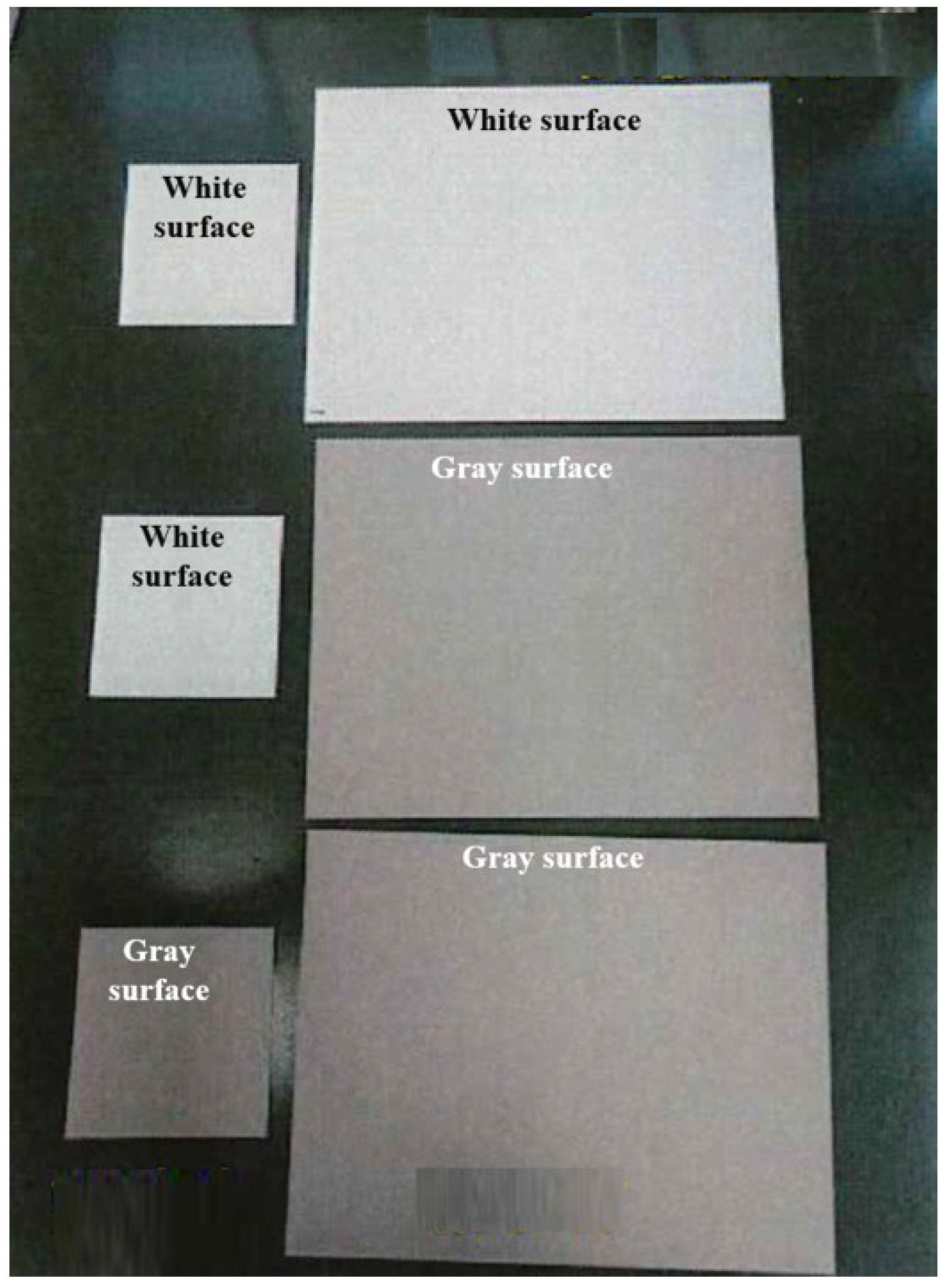
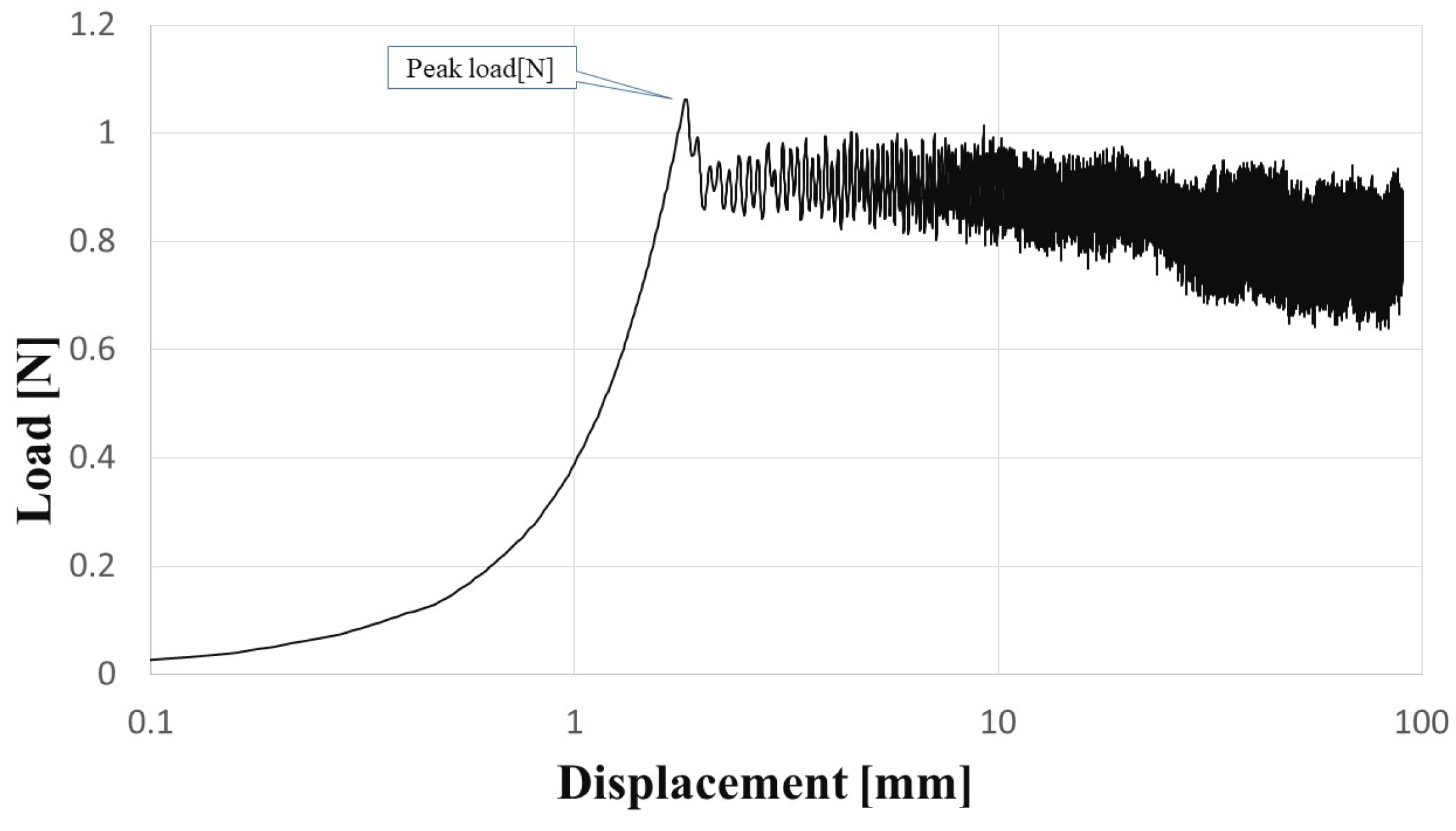
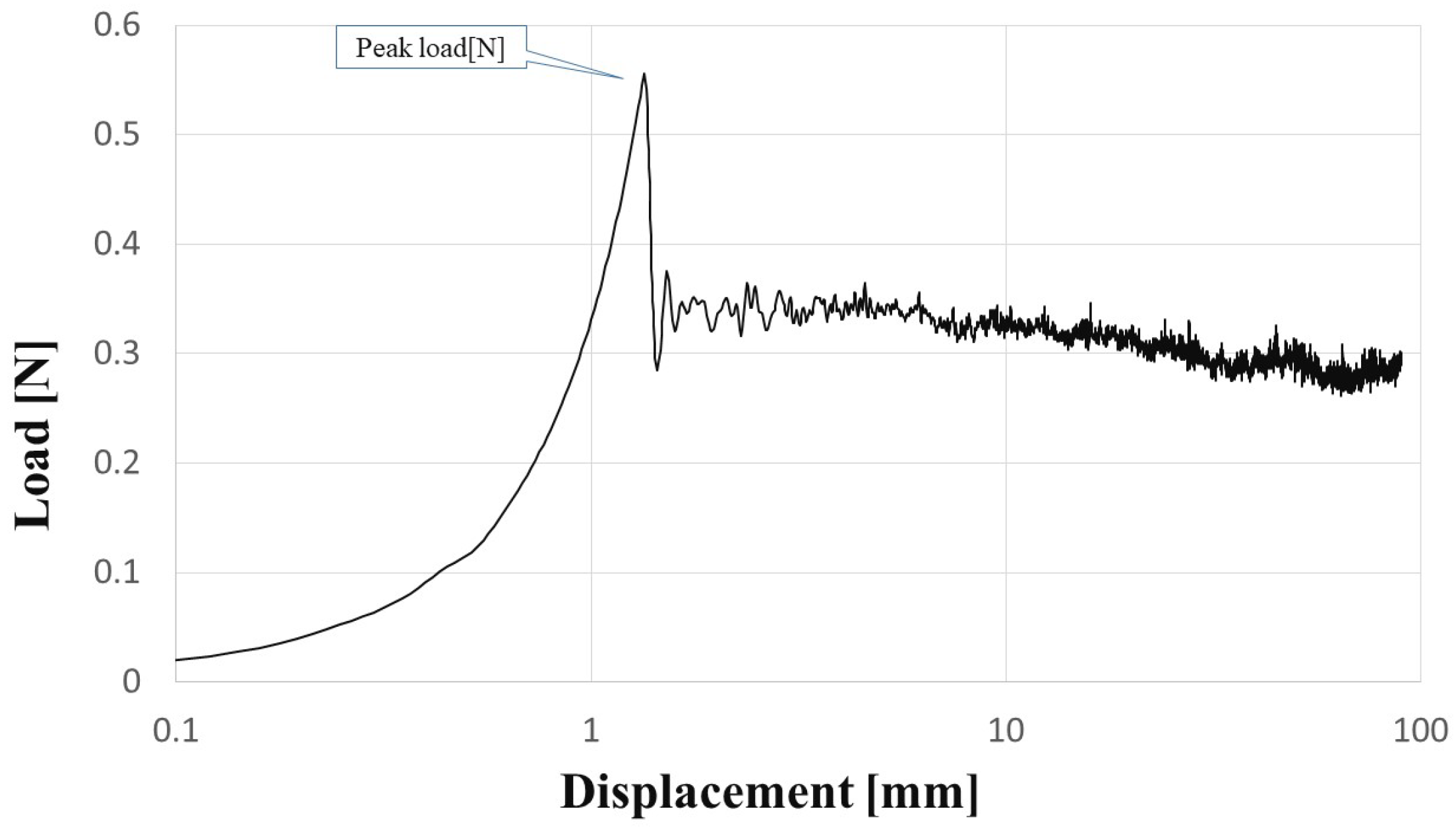
The paper used to fabricate the paper craft aerial acrobat robot in this research is cardboard manufactured by JOHOKU (model number  W B 3 10 g _ T _ A 3 5 0 x ) [24]. This paper has a thickness of approximately 0.4 mm and a density of 310 g/m2. Its surface is coated white, while the back side is uncoated and gray. Therefore, as shown in Figure 23, both the static and kinetic coefficients of friction are measured for three combinations: white surface/white surface, white surface/gray surface, and gray surface/gray surface.
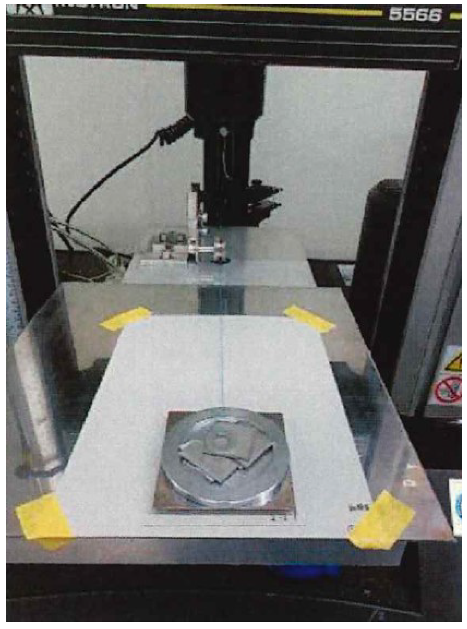
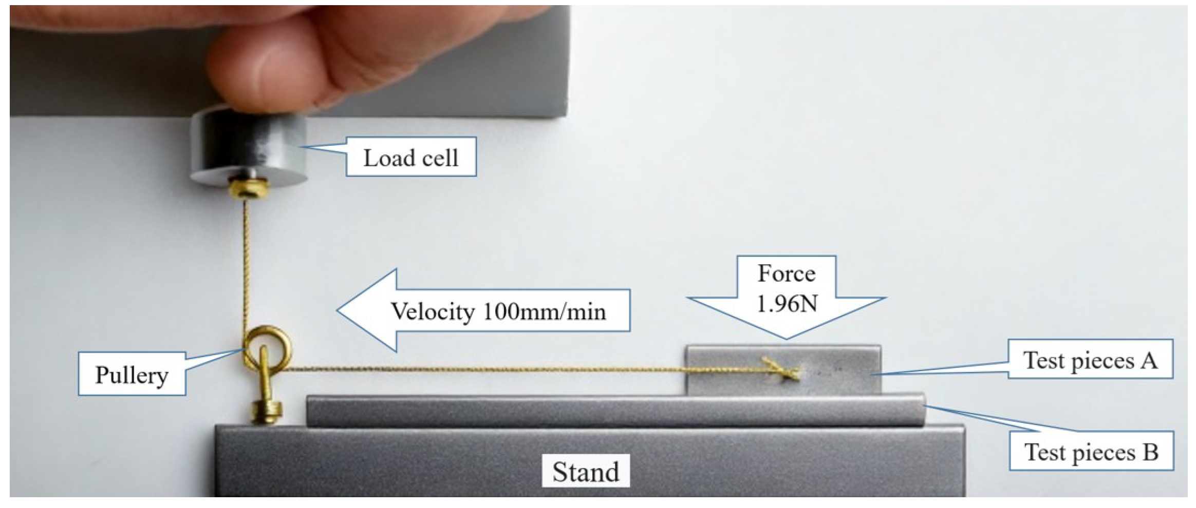
Figure 24 shows the setup of the friction test. The testing machine is the INSTRON 5566 [25]. The friction test conditions are summarized in Table 2. A schematic diagram of the test setup is shown in Figure 25. As illustrated, two paper specimens are placed in contact, and a test mass is applied on top. A spring is connected to a load cell, which is in turn connected to the upper test piece via a pulley system. The upper specimen is pulled by a string, and the resulting resistance force (friction force) is measured by the load cell.
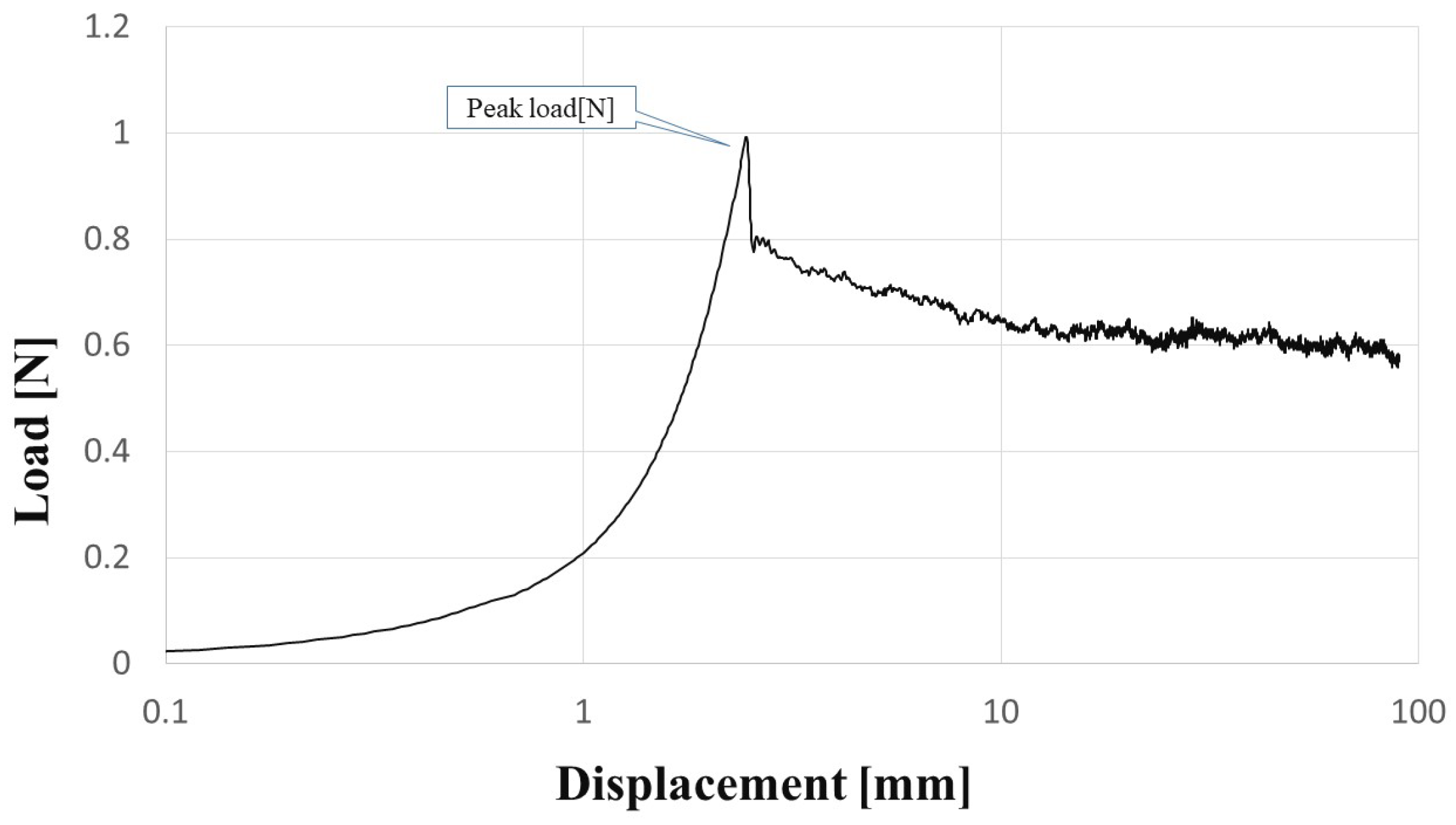
As shown in Figure 26 (white surface/white surface), the horizontal and vertical axes represent displacement [mm] and load [N], respectively. The displacement values on the horizontal axis are presented on a logarithmic scale. The results obtained from the graph are summarized in Table 3. As the load cell moves, the spring force builds up until the static friction limit is reached. Additionally, the force applied by the spring increases as the load cell moves. Eventually, this force exceeds the frictional force, and the test pieces begin to slide relative to each other. The coefficient of static friction (white surface/white surface) is obtained as follows:
μ S = F S F F = 0.993 1.96 = 0.507
The friction force is calculated by the load mean value of the relative displacement motion (stick-slip motion) between the contact surfaces. In the calculation of the kinetic friction force, the peak  F S  of static friction force is ignored.
μ K = F K F F = 0.661 1.96 = 0.337
The example calculation using the above formula gives the kinetic friction coefficient between the white surface and the white surface, as shown in Table 3. Similar results for other surface combinations can be obtained, as shown in Figure 27 and Figure 28. In this study, the arm and handrail are made of paper, with the arm’s white surface coming into contact with the gray surface of the handrail. Therefore, the static and kinetic friction coefficients for the white surface/gray surface combination in Table 3 are applied to the analysis model of the paper craft aerial acrobat robot prototype.

7. Validation of Multibody Dynamics Modeling Through Comparison with Mechanical Theory and Image-Based Measurements

7.1. Comparison of Methods

Table 4 summarizes and compares the modeling approaches used for the aerial acrobatic robot, namely the quasi-static single-link model (Nishibori theory), the dynamic two-link analytical model, and the general multibody dynamics formulation. The comparison clarifies the underlying assumptions, degrees of freedom, treatment of inertia, and applicability domains of each approach. In particular, the quasi-static model is shown to be suitable for simplified torque estimation under negligible inertial effects, whereas the proposed two-link model explicitly accounts for dynamic coupling and angular accelerations. The multibody dynamics approach provides the most comprehensive representation, including contact, friction, and elastic elements, at the cost of increased computational complexity. The modeling approach adopted in the dynamic two-link analytical model is based on the following assumptions.
(1)
The swing frame and robot body are modeled as rigid bodies, and elastic deformation of the paper structures is neglected, as it is sufficiently small compared to the overall rotational motion.
(2)
The system motion is assumed to be planar, and out-of-plane motion is ignored.
(3)
Friction is considered only in the multibody dynamics simulations, while it is neglected in the analytical two-link model to focus on fundamental dynamic behavior.
(4)
Air drag is not included in both the quasi-static single-link model and the MBD; its influence is evaluated by the dynamic two-link model and shown to have a negligible effect on angular acceleration.
(5)
The quasi-static single-link model is applicable only when inertial effects of robot are negligible, whereas the dynamic two-link model is required when the inertial effects of robot become significant.
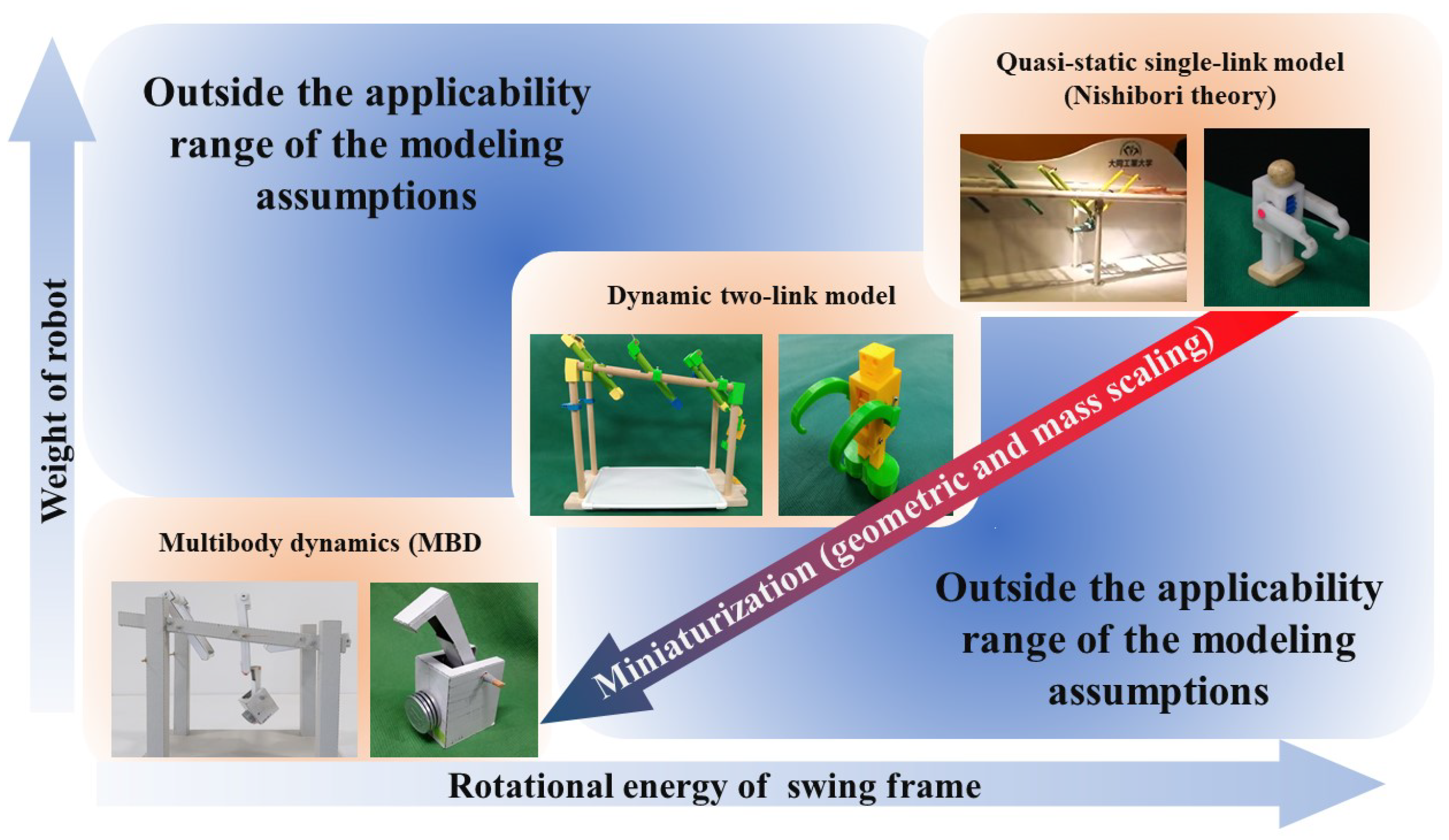
Figure 29 illustrates the applicability domains of different modeling approaches for the aerial acrobatic robot, mapped with respect to the robot weight and the rotational energy of the swing frame. The quasi-static single-link model (Nishibori theory) is applicable in a limited region where the robot is relatively heavy and the rotational energy of the swing frame is sufficiently large. In this regime, inertial effects are small compared to gravitational torque, and the motion can be approximated by a quasi-static balance of moments. As the robot becomes lighter and the available rotational energy decreases, dynamic effects such as link inertia and interaction between multiple links become increasingly significant. In this intermediate region, represented by the dynamic two-link model proposed in this study, angular accelerations of different links may exhibit opposite signs, which cannot be captured by the static torque-based formulation. For lightweight robots operating under low-energy conditions and involving contact, friction, and time-varying constraints, a full multibody dynamics (MBD) approach is required. In this domain, the assumptions underlying the quasi-static model are violated, and numerical time integration of the equations of motion becomes essential. The shaded regions labeled as “Outside applicability range of the models” indicate parameter ranges where simplified models fail to predict stable traversal motion, highlighting the necessity of selecting an appropriate modeling methodology according to the system scale and dynamic characteristics.

7.2. Angles  θ 1  and  θ 2

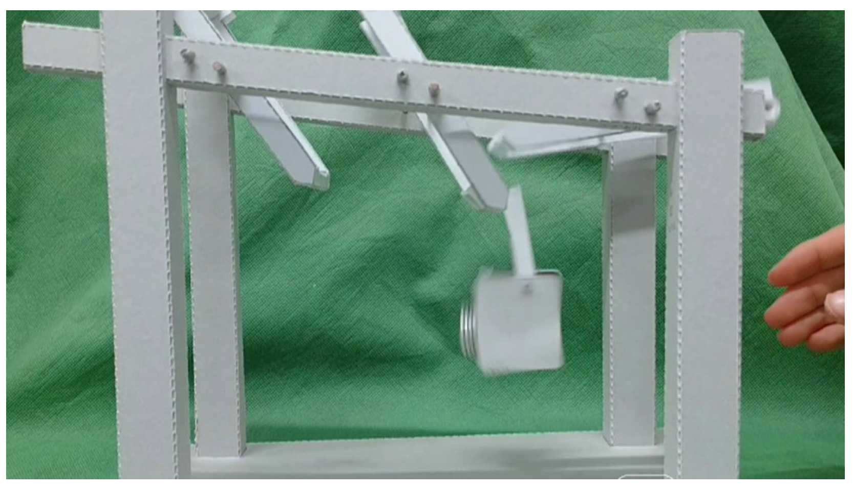
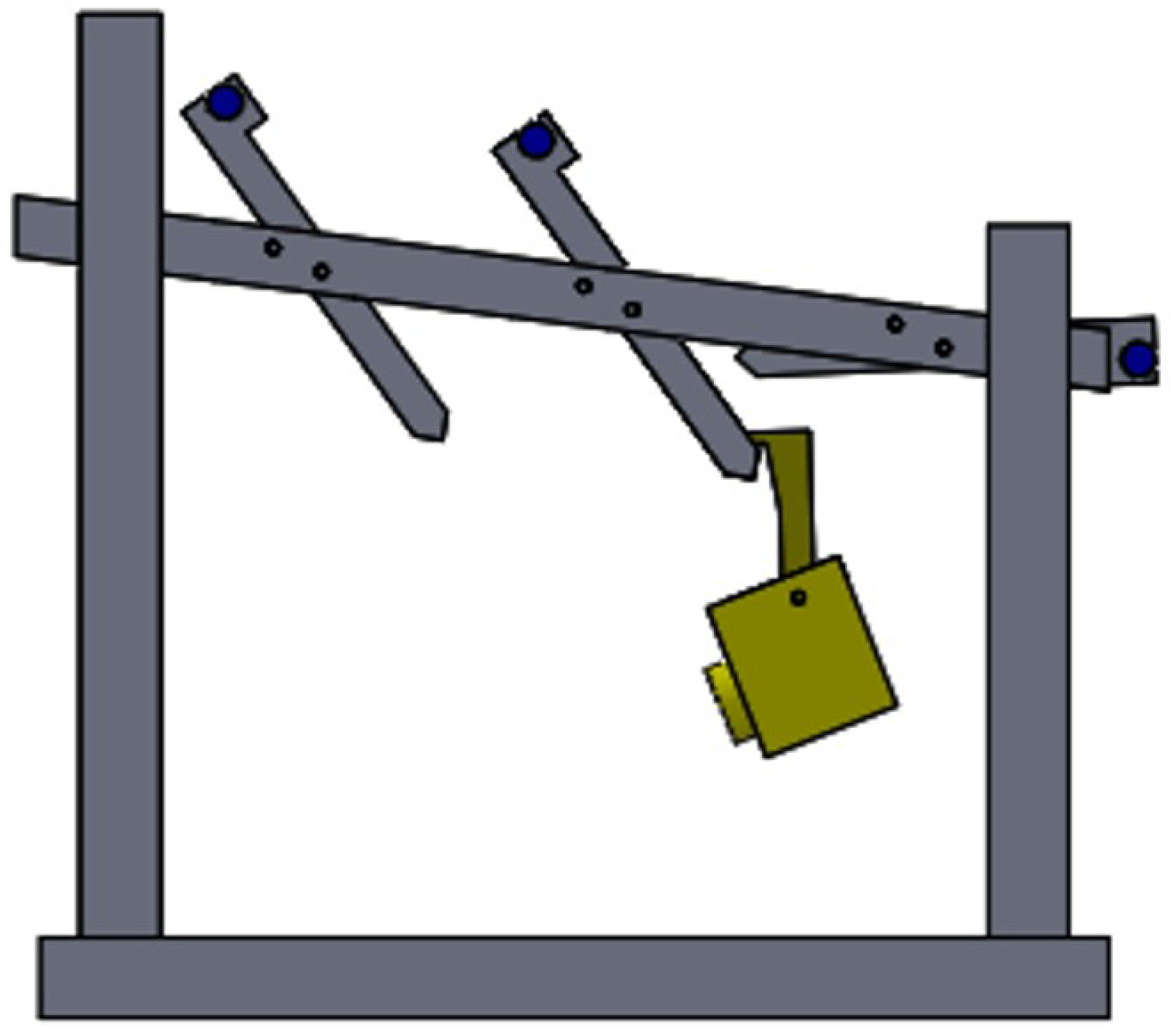
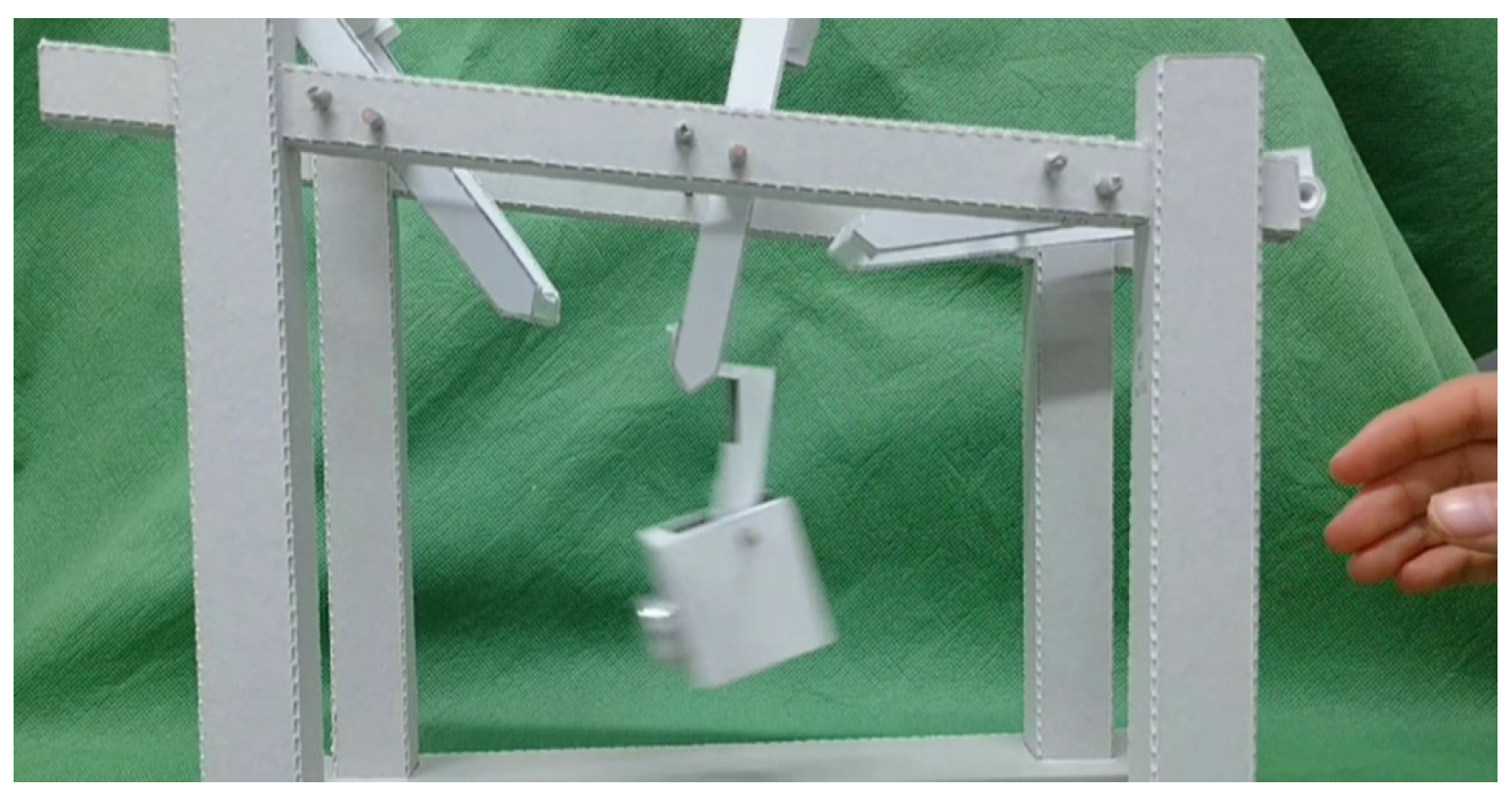
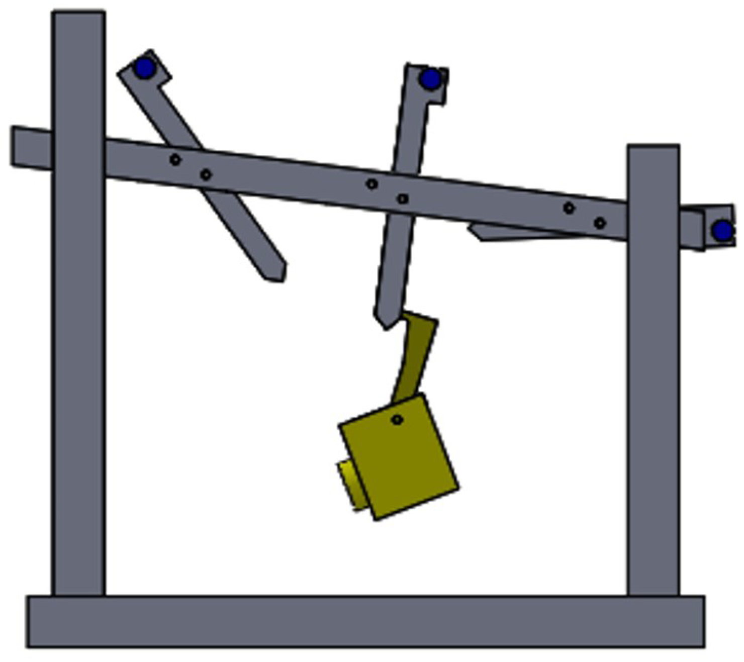
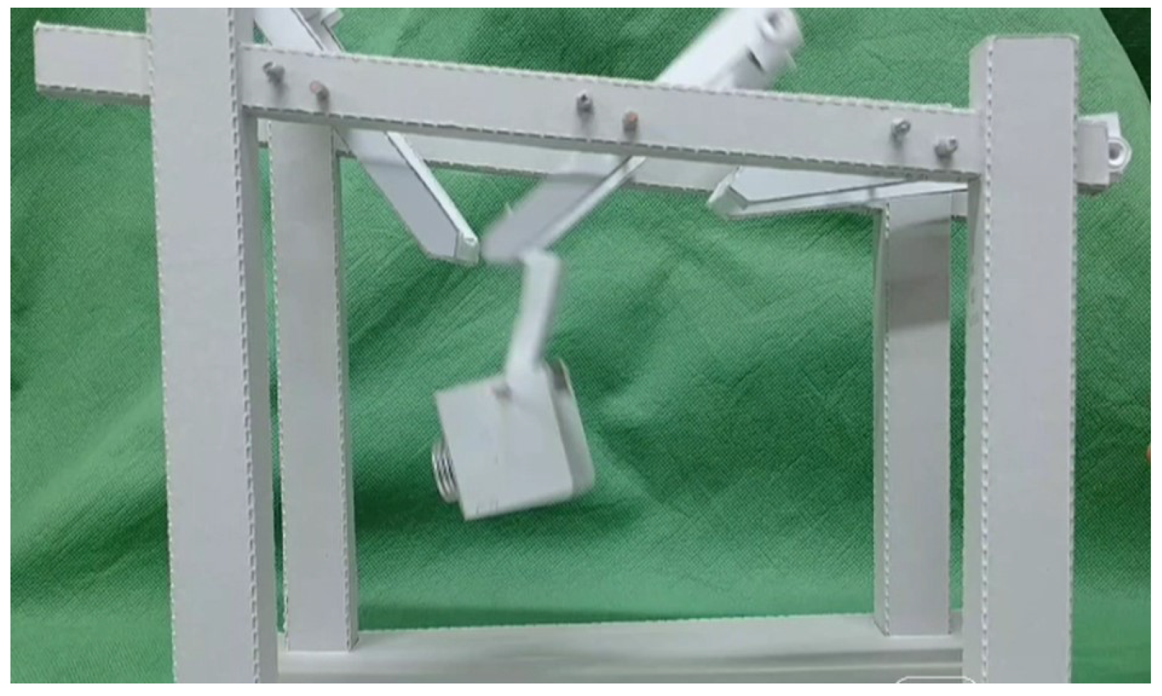
Figure 30, Figure 31, Figure 32, Figure 33, Figure 34, Figure 35, Figure 36, Figure 37 and Figure 38 show the actual movement of the robot from 0 [s] to 0.62 [s]. Similarly, Figure 31, Figure 32, Figure 33, Figure 34, Figure 35, Figure 36, Figure 37, Figure 38 and Figure 39 illustrate the movement based on multibody dynamics. The operation completes in approximately 0.62 s for one swing cycle.
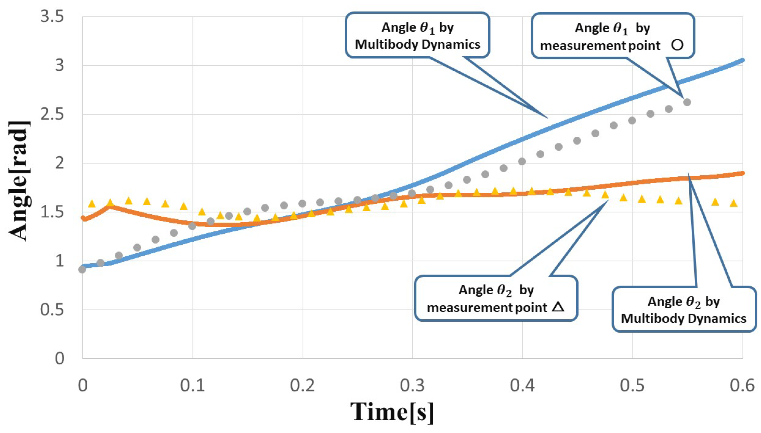
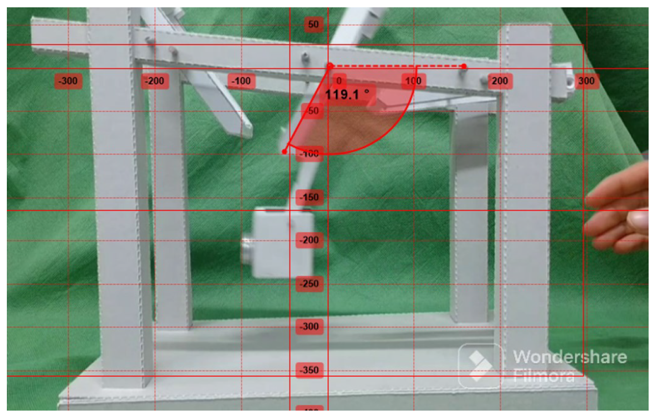
The angle between the horizontal direction and the swing frame is defined as  θ 1 , and the angle between the horizontal direction and the robot’s arm is defined as  θ 2 . As shown in Figure 17, the system is simplified as the two-link model with kinematic constraints. Figure 40 shows the time variation in the angles  θ 1  and  θ 2 . The solid lines in Figure 40 represent the changes in  θ 1  and  θ 2  based on multibody dynamics. The circles ◯ and triangles △ in Figure 40 indicate the measured points of  θ 1  and  θ 2 , respectively, obtained using Kinovia to measure the time variation in the angles [20].
As shown in Figure 41, these values are calculated by extracting the angles at each time point from a video recording using Kinovea.
The angle  θ 1 , both in measurement and analysis, starts from an initial angle of approximately  55  and increases monotonically over time. Subsequently, since the robot’s arm detaches from the handrail of the swing frame, there is no change in  θ 1  after approximately 0.62 s. These angular results show close agreement between the analysis and the actual motion of the swing frame, indicating that the modeling approach based on multibody dynamics accurately represents the actual behavior.
For the angle  θ 2 , both in measurement and analysis, the initial angle starts from approximately  80 . Assuming that the swing frame is stationary, the robot’s arm tends to align with the gravity vector due to gravitational torque, resulting in  θ 2 90 . When the angle  θ 1  of the swing frame changes over time, the angle  θ 2  increases or decreases around  θ 2 90  due to the influence of the robot’s mass, with the connection point between the handrail and the arm acting as the pivot. In other words, it can be observed that the robot swings left and right around the connection point while the swing frame is in motion. This trend is similarly confirmed in the measurements.

7.3. Angular Velocities  θ ˙ 1  and  θ ˙ 2

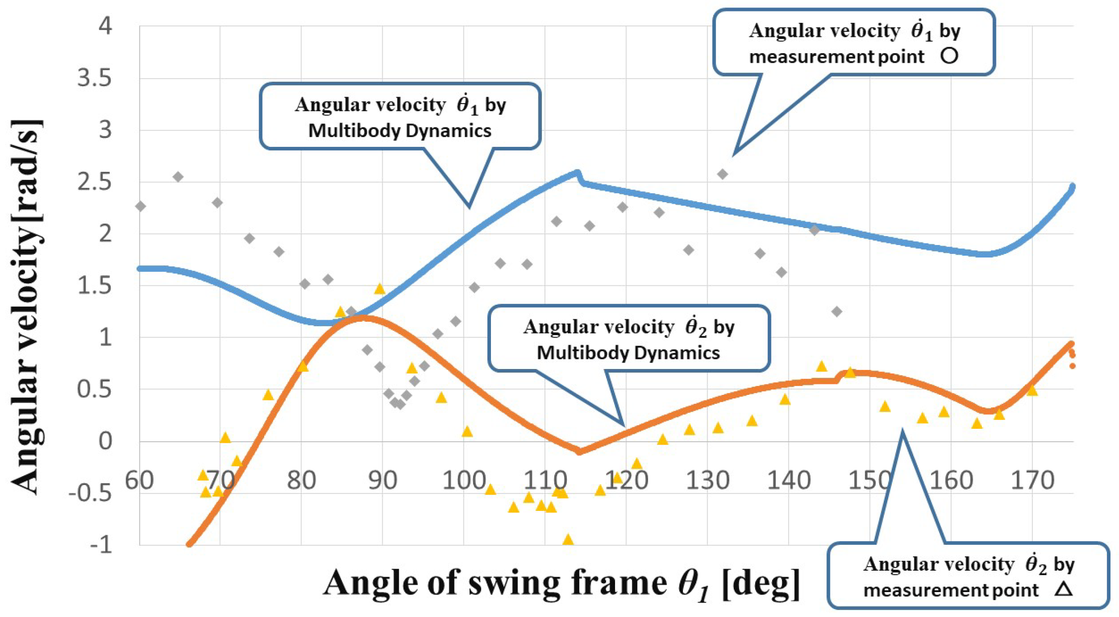
Figure 42 shows a graph with the swing frame angle  θ 1  on the horizontal axis and angular velocity on the vertical axis. The circles (◯) indicate measurement points of the swing frame’s angular velocity  θ ˙ 1  (see Figure 17), while the triangles (△) represent measurement points of the arm’s angular velocity  θ ˙ 2 . The solid lines show the result of multibody dynamics analysis. The initial swing frame angle is approximately  θ 1 55 . At this point, the robot’s arm slips off the handrail of the preceding swing frame, collides with the handrail of the next swing frame, and then catches on it. This moment is defined as the start of the motion, after which the swing frame begins to rotate. From that moment, the swing frame begins to rotate. The angle  θ 1  increases and eventually reaches approximately  180 , at which point the swing frame stops rotating. Before  θ 1  reaches approximately  180 , the robot’s arm slips off the handrail, causing the robot to fall downward. Subsequently, the arm collides with and catches on the handrail of the next swing frame. This sequence of events is repeated across the series of swing frames. According to the simulation data, when  θ 1  reaches approximately  80 , the angular velocity of the swing frame  θ 1 ˙  decreases to around 1.1 [rad/s]. At this point, the angular velocity  θ 2 ˙  of the robot increases in the positive rotational direction. However,  θ 1 ˙  remains positive, indicating that the swing frame continues to rotate forward. In the measured data, a similar trend is observed to that obtained from the multibody dynamics analysis. Specifically, when the angle  θ 1  is less than about  90 θ 1 ˙  decreases while  θ 2 ˙  increases. Conversely, when the angle  θ 1  is greater than about  90 θ 1 ˙  increases while  θ 2 ˙  decreases. The discrepancy between the simulation results and the measurement data is likely due to the limited accuracy inherent in image-based analysis. In addition, the simulation using multibody dynamics does not account for factors such as air resistance, elastic deformation of the swing frame, dimensional inaccuracies, or friction between the bamboo skewer used as the axis and the paper-made shaft hole. These unmodeled effects are considered to contribute to the differences between the calculated and measured data. Nevertheless, the order of magnitude of the angular velocities from both the measurements and the simulation shows good agreement. The average angular velocity  θ ˙ 1  obtained from image-based measurement is 1.5 rad/s, while that from the multibody dynamics simulation is 1.7 rad/s, indicating a close match. Both the simulation and measurement data show that, although some fluctuation exists around the average value, the angular velocity  θ ˙ 1  remains positive and relatively stable throughout the motion.

7.4. Angular Accelerations  θ ¨ 1  and  θ ¨ 2  

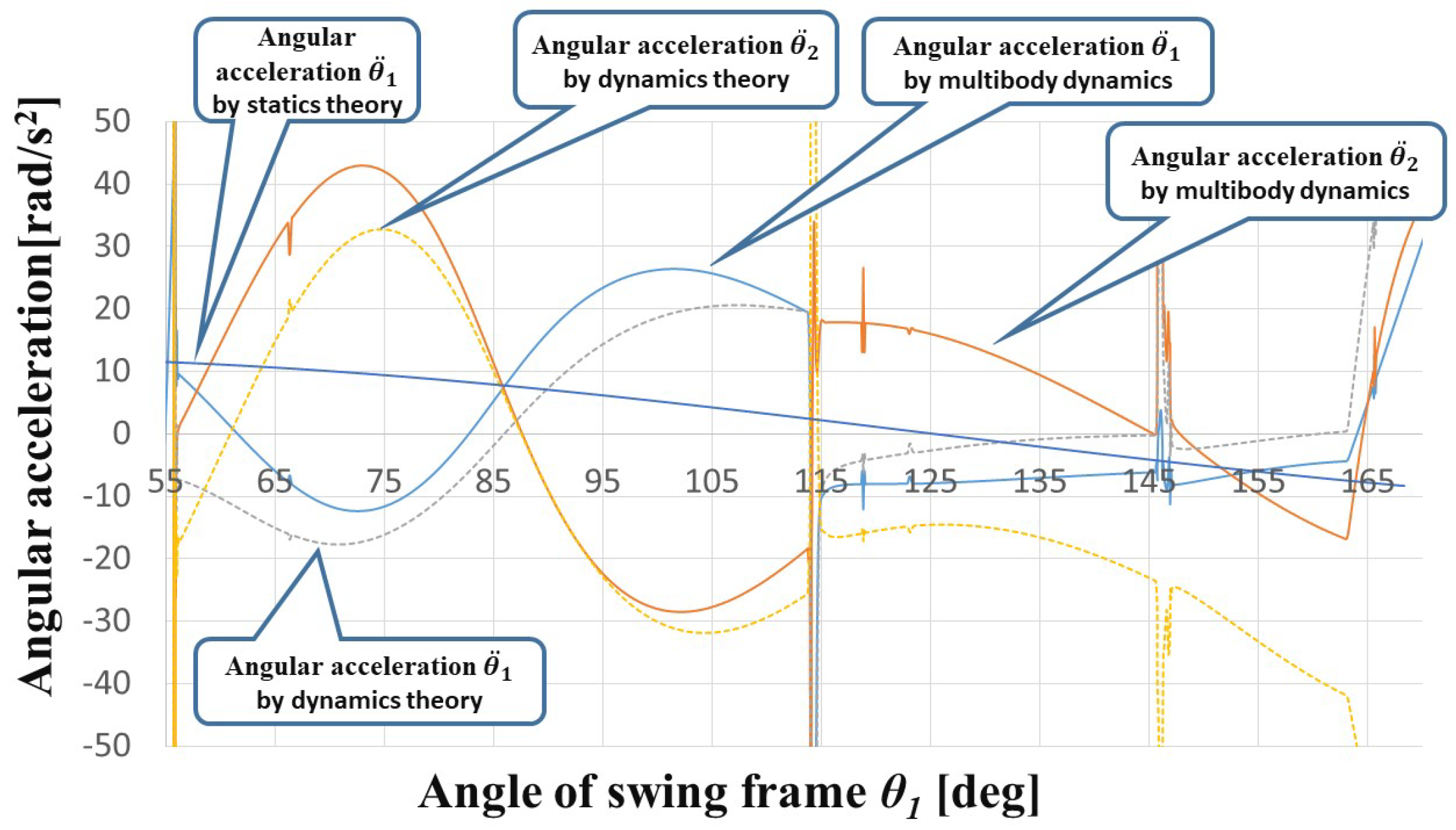
To enable the aerial acrobat robot to operate, it is necessary to maintain a positive angular acceleration  θ ¨ 1  in the forward direction for as long as possible. Figure 43 shows a graph with the swing frame angle  θ 1  [deg] on the horizontal axis and the angular accelerations  θ ¨ 1  and  θ ¨ 2  [rad/ s 2 ] on the vertical axis Detailed data and simulation results are provided in the section of Supplementary Materials. The initial angles are approximately  θ 1 55  and  θ 2 81 , and the corresponding time is defined as  t 0  s. At this moment, the robot’s hand comes into contact with the handrail, initiating the rotation of the swing frame. The arm slips off the handrail at approximately  θ 1 165  and the corresponding time is  t = 0.62  s. Throughout the entire range of  θ 1 , the theoretical angular acceleration values  θ ¨ 1  and  θ ¨ 2  obtained from the double-pendulum model (Equations (A25) and (A30)) closely match the results from the multibody dynamics simulation based on Equation (A72).
In the region where the swing frame angle  θ 1  ranges from approximately  55  to  125 , the conventional evaluation formula (Equation (1)) yields a consistently positive angular acceleration. In contrast, the result from the multibody dynamics analysis (Equation (A72)) shows a transition from positive to negative angular acceleration, and then back to positive. In the region where the swing frame angle  θ 1  ranges from approximately  55  to  90 , the counterbalance is lifted upward. When the counterbalance moves against gravity, the length h effectively becomes shorter between the counterbalance and the rotational axis of the swing frame. This suppresses the negative moment caused by the counterbalance. Around  θ 1 115  in the curve derived from the multibody dynamics analysis, a discontinuity appears in the angular acceleration waveform, and in the multibody dynamics simulation result, the moment suddenly shifts from positive to negative. This discontinuity is caused by a slight shift in the contact position between the robot’s arm and the handrail, which results in a small change in the effective lever arm length used for calculating the moment. At the same time, the raised counterbalance begins to exert a force in the downward direction due to gravity, contributing to a positive rotational moment. When the counterbalance moves in the same direction as the direction of gravity, the length h effectively becomes longer between the axis of rotation of the swing frame and the counterbalance. Due to the effect of the counterbalance, the robot is lifted against the gravity direction. According to the theoretical calculation based on the conventional evaluation formula (Equation (1)), the angular acceleration remains positive up to around  θ 1 125 , and becomes consistently negative thereafter. Since the angular acceleration becomes predominantly negative beyond this angle, the angular velocity of the swing frame tends to decrease. The theoretical analysis incorporating aerodynamic drag moments is conducted to evaluate their influence on the system dynamics. The results show that the inclusion of drag-induced moments does not produce a noticeable difference in the time histories of the angular accelerations of both angles,  θ 1  and  θ 2 , compared with the model without aerodynamic drag. This indicates that, under the operating conditions considered in this study, the effect of aerodynamic drag on the angular acceleration responses is negligible.

8. Conclusions

Based on the design of a conventional large-scale swing toy made of resin, a lightweight and compact paper-based version, referred to as the “Paper Craft Aerial Acrobatic Robot,” was developed to improve accessibility and ease of fabrication. In this robot, locomotion across a series of swing frames is achieved by converting gravitational potential energy into rotational motion of the frames, without the use of electrical actuators. However, the significant reduction in size introduces new challenges, including insufficient rotational motion and increased sensitivity to inertial effects.
To clarify these issues, the traversal motion of the aerial acrobatic robot was analyzed using a multibody dynamics (MBD) framework, and the rotational moment of the swing frame was examined in detail. A clear discrepancy was identified between the conventional quasi-static evaluation method (Nishibori theory), which was effective for large-scale systems, and the results obtained from dynamic analysis, particularly in the time history of angular acceleration. To investigate the origin of this discrepancy, the swing frame and the robot were modeled as a two-link mechanism, and the angular acceleration of the swing frame was derived using the Euler–Lagrange equations of motion. The results were further compared with those obtained from the governing equations of the multibody system, showing consistent trends between the analytical and numerical approaches.
The multibody dynamics results showed good agreement with image-based experimental measurements. A key finding is that the angular accelerations of the swing frame and the robot arm frequently exhibit opposite signs, a dynamic behavior that is fundamentally not captured by the quasi-static evaluation formula. Because the quasi-static approach assumes a unidirectional contribution of angular acceleration to the rotational moment, it can significantly overestimate the effective rotational force, depending on the mass balance between the counterweight and the robot body.
From an engineering design perspective, these results provide several practical guidelines. First, quasi-static torque-based design methods are inadequate for lightweight, low-inertia systems in which dynamic coupling between links is significant. Second, explicit consideration of angular acceleration and inertial effects is essential for accurately predicting motion in miniaturized passive mechanisms. Third, dynamic models with multiple degrees of freedom, such as two-link or multibody formulations, should be employed when designing systems that involve large-amplitude rotational motion and intermittent contact. These guidelines clarify the conditions under which quasi-static design approaches break down and dynamic modeling becomes necessary.
As future work, the proposed modeling framework will be extended to incorporate additional physical effects, such as structural flexibility, contact compliance, and frictional nonlinearity. In addition, systematic parametric studies based on the developed analytical and MBD models will be conducted to derive more generalized and quantitative design guidelines for achieving stable and expressive motion. These extensions are expected to contribute to the systematic design of lightweight, energy-efficient robotic mechanisms not only for entertainment applications, but also for broader engineering domains.

Supplementary Materials

The following supporting information can be downloaded at: https://www.mdpi.com/article/10.3390/app16020921/s1. Calculation data and angular acceleration profiles.

Author Contributions

Conceptualization, K.N. and K.S.; Methodology, K.S.; Software, K.S.; Formal analysis, K.S.; Investigation, K.S.; Data curation, K.S.; Validation, K.S. and K.N.; Visualization, K.S.; Writing—original draft preparation, K.S.; Writing—review and editing, K.N. and K.S.; Supervision, K.N.; Project administration, K.S.; Funding acquisition, K.S. All authors have read and agreed to the published version of the manuscript.

Funding

This research received no external funding.

Institutional Review Board Statement

Not applicable.

Informed Consent Statement

Not applicable.

Data Availability Statement

Data are contained within the article.

Conflicts of Interest

The authors declare no conflicts of interest.

Appendix A. Lagrangian Equations of Motion

The equations of motion for the two-link mechanism shown in Figure 17 are derived using the Lagrangian L. The center of mass position of the swing frame is given by the following equation.
( x 1 , y 1 ) = ( 0 , 0 )
The center of mass position of the robot is given by the following equation.
( x 2 , y 2 ) = ( L b cos θ 1 L c cos θ 2 , L b sin θ 1 L c sin θ 2 )
The center of mass position of the counterbalance is given by the following equation.
( x 3 , y 3 ) = ( L a cos θ 1 h sin θ 1 , L a sin θ 1 + h cos θ 1 )
The translational velocity at the center of mass of the swing frame is given by the following equation.
( x 1 ˙ , y 1 ˙ ) = ( 0 , 0 )
The translational velocity at the center of mass of the robot is given as follows.
( x 2 ˙ , y 2 ˙ ) = ( L b θ 1 ˙ sin θ 1 + L c θ 2 ˙ sin θ 2 , L b θ 1 ˙ cos θ 1 L c θ 2 ˙ cos θ 2 )
The translational velocity at the center of mass of the counterbalance is given as follows.
( x 3 ˙ , y 3 ˙ ) = ( L a θ 1 ˙ sin θ 1 h θ 1 ˙ cos θ 1 , L a θ 1 ˙ cos θ 1 h θ 1 ˙ sin θ 1 )
The magnitude of the translational velocity at the center of mass of the swing frame is obtained by the following equation.
v 1 = ( x 1 ˙ ) 2 + ( y 1 ˙ ) 2 = 0
The magnitude of the translational velocity at the center of mass of the robot is given as follows.
v 2 = ( x 2 ˙ ) 2 + ( y 2 ˙ ) 2 = ( L b θ 1 ˙ sin θ 1 + L c θ 2 ˙ sin θ 2 ) 2 + ( L b θ 1 ˙ cos θ 1 + L c θ 2 ˙ cos θ 2 ) 2 = L b 2 θ 1 ˙ 2 + L c 2 θ 2 ˙ 2 + 2 L b L c θ 1 ˙ θ 2 ˙ cos ( θ 1 θ 2 )
In the above equation, the trigonometric addition formula is applied during the derivation. The magnitude of the translational velocity at the center of mass of the counterbalance is given as follows.
v 3 = ( x 3 ˙ ) 2 + ( y 3 ˙ ) 2 = ( L a θ 1 ˙ sin θ 1 + h θ 1 ˙ cos θ 1 ) 2 + ( L a θ 1 ˙ cos θ 1 h θ 1 ˙ sin θ 1 ) 2 = L a 2 θ 1 ˙ 2 + h 2 θ 1 ˙ 2 = | θ 1 ˙ | L a 2 + h 2
The total kinetic energy K, which consists of the translational and rotational kinetic energies of the swing frame, the robot, and the counterbalance, is given as follows.
K = 1 2 m 1 v 1 2 + 1 2 m 2 v 2 2 + 1 2 m 3 v 3 2 + 1 2 I 1 θ 1 ˙ 2 + 1 2 I 2 θ 2 ˙ 2 + 1 2 I 3 θ 3 ˙ 2
The variable  θ 3  represents the rotational angle of the counterbalance. However, in this study, the counterbalance is assumed to be a point mass. Therefore, it does not undergo rotational motion itself. Based on this assumption, the following equation is introduced.
θ 3 = 0
θ 3 ˙ = 0
The swing frame is modeled as a line. The swing frame consists of two vertical support columns arranged symmetrically on the left and right, which integrally connect the counterbalances located at the ends of the frame. Its moment of inertia  I 1  is approximated by the following equation.
I 1 = 2 L b L a l 2 ρ d V + I 3 = 2 L b L a l 2 m 1 V d V + I 3 = 2 m 1 ( L a + L b ) A L b L a l 2 A d l + I 3 = 2 m 1 L a + L b 1 3 l 3 L b L a + I 3 = 2 m 1 ( L a 3 + L b 3 ) 3 ( L a + L b ) + I 3 = 2 m 1 3 ( L a 2 + L b 2 L a L b ) + I 3
In the above equation, the variable  ρ  represents the density,  d V  denotes the infinitesimal volume, A is the cross-sectional area of the swing frame, and  d l  represents the infinitesimal length along the longitudinal direction of the swing frame.  L c  denotes the length of the arm, and  L d  represents the distance from the rotation center to the bottom of the torso. The rotation center is defined as the contact point between the arm and the handrail of the swing frame, while the torso containing the weight is offset from this rotation center. Although the robot has joints at the torso and the arm, it is modeled as a single line to simplify the mathematical model. The moment of inertia  I 2  is approximated by the following equation.
I 2 = L c L d l 2 ρ d V = L c L d l 2 m 2 V d V = L c L d l 2 m 2 ( L d L c ) A A d l = m 2 L d L c 1 3 l 3 L c L d = m 2 3 ( L d 2 + L d L c + L c 2 )
Here,  d l  represents an infinitesimal length along the longitudinal direction of the line modeling the robot. The moment of inertia of the counterbalance about the rotation axis is derived by assuming it as a point mass.
I 3 = m 3 L a 2 + h 2 2 = m 3 ( L a 2 + h 2 )
The potential energy P at the center of mass of the robot and the counterbalance is given as follows.
P = m 2 g ( L b sin θ 1 + L c sin θ 2 ) + m 3 g ( L a sin θ 1 + h cos θ 1 )
Note that the signs of the gravitational potential terms depend on the definition of the coordinate system. Since the center of mass of the swing frame is located at the origin, it is assumed that the swing frame has no potential energy. The Lagrangian L is given as follows.
L = K P = 1 2 m 1 v 1 2 + 1 2 m 2 v 2 2 + 1 2 m 3 v 3 2 + 1 2 I 1 θ 1 ˙ 2 + 1 2 I 2 θ 2 ˙ 2 + m 2 g ( L b sin θ 1 + L c sin θ 2 ) m 3 g ( L a sin θ 1 + h cos θ 1 )
Substituting Equations (A7)–(A9) into the Lagrangian L gives the following equation.
L = 1 2 m 2 L b 2 θ 1 ˙ 2 + L c 2 θ 2 ˙ 2 + 2 L b L c θ 1 ˙ θ 2 ˙ cos ( θ 1 θ 2 ) + 1 2 m 3 θ 1 ˙ 2 ( L a 2 + h 2 ) + 1 2 I 1 θ 1 ˙ 2 + 1 2 I 2 θ 2 ˙ 2 + m 2 g ( L b sin θ 1 + L c sin θ 2 ) m 3 g ( L a sin θ 1 + h cos θ 1 )
Taking the partial derivative of the Lagrangian L with respect to the angular velocity  θ 1 ˙  gives the following equation.
L θ 1 ˙ = m 2 L b 2 θ 1 ˙ + m 2 L b L c θ 2 ˙ cos ( θ 1 θ 2 ) + m 3 θ 1 ˙ ( L a 2 + h 2 ) + I 1 θ 1 ˙
The following equation is obtained by differentiating the above equation with respect to time t.
d d t L θ 1 ˙ = { m 2 L b 2 + m 3 ( L a 2 + h 2 ) + I 1 } θ 1 ¨ + m 2 L b L c cos ( θ 1 θ 2 ) θ 2 ¨ m 2 L b L c θ 2 ˙ ( θ 1 ˙ θ 2 ˙ ) sin ( θ 1 θ 2 )
Taking the partial derivative of the Lagrangian L with respect to the angle  θ 1  gives the following equation.
L θ 1 = m 2 L b L c θ 1 ˙ θ 2 ˙ sin ( θ 1 θ 2 ) + m 2 g L b cos θ 1 m 3 g L a cos θ 1 + m 3 g h sin θ 1
Taking the partial derivative of the Lagrangian L with respect to the angular velocity  θ 2 ˙  gives the following equation.
L θ 2 ˙ = m 2 L c 2 θ 2 ˙ + m 2 L b L c θ 1 ˙ cos ( θ 1 θ 2 ) + I 2 θ 2 ˙
Differentiating the above equation with respect to time t yields the following equation.
d d t L θ 2 ˙ = m 2 L b L c cos ( θ 1 θ 2 ) θ 1 ¨ + ( m 2 L c 2 + I 2 ) θ 2 ¨ m 2 L b L c θ 1 ˙ ( θ 1 ˙ θ 2 ˙ ) sin ( θ 1 θ 2 )
Taking the partial derivative of the Lagrangian L with respect to the angle  θ 2  gives the following equation.
L θ 2 = m 2 L b L c θ 1 ˙ θ 2 ˙ sin ( θ 1 θ 2 ) + m 2 g L c cos θ 2
From the Lagrangian equation of motion with respect to the angle  θ 1 , the following equation is obtained.
d d t L θ 1 ˙ L θ 1 τ 1 = η 1 θ 1 ¨ + η 2 θ 2 ¨ + η 3 = 0
Here,  τ 1  denotes the generalized force corresponding to the generalized coordinate  q i . When the generalized coordinate is the rotational angle,  τ 1  physically represents the moment acting on the system. Since the generalized coordinate  θ  is dimensionless, the partial derivative  L θ  has the dimension of energy (N·m), which is equivalent to moment (N·m), ensuring dimensional consistency in the Lagrange equation. Aerodynamic drag is a non-conservative force and therefore cannot be included in the Lagrangian. Instead, the drag moment is introduced as a generalized force in the Lagrange equations. The drag moment is modeled as a quadratic function of angular velocity, which is a common approximation for rotational motion in air [26,27,28].
τ 1 = 0 L a 1 2 ρ C d A ( v 1 + l θ 1 ˙ ) v 1 + l θ 1 ˙ · l · d l 0 L b 1 2 ρ C d A ( v 1 + l θ 1 ˙ ) v 1 + l θ 1 ˙ · l · d l = 1 2 ρ C d A θ 1 ˙ θ 1 ˙ 0 L b l 3 d l 1 2 ρ C d A θ 1 ˙ θ 1 ˙ 0 L a l 3 d l = 1 8 ρ C d A θ 1 ˙ θ 1 ˙ ( L a 4 + L b 4 )
The aerodynamic drag moment acting on the swing frame is evaluated by integrating the distributed drag force along the link length l from a joint (See Figure 17). A denotes the projected cross-sectional area of the link subjected to aerodynamic forces.  ρ  represents the air density, and  C d  is the drag coefficient (See Table 1). As shown in Equation (A1),  v 1  is equal to zero. The negative sign indicates that the aerodynamic drag moment always acts in the direction opposite to the angular velocity, thereby dissipating mechanical energy.
The variables  η 1  to  η 3  in the above equation are given by the following equations.
η 1 = m 2 L b 2 + m 3 ( L a 2 + h 2 ) + I 1
η 2 = m 2 L b L c cos ( θ 1 θ 2 )
η 3 = m 2 L b L c θ 2 ˙ 2 sin ( θ 1 θ 2 ) m 2 g L b cos θ 1 + m 3 g L a cos θ 1 m 3 g h sin θ 1 τ 1
From the Lagrangian equation of motion with respect to the angle  θ 2 , the following equation is obtained.
d d t L θ 2 ˙ L θ 2 τ 2 = η 4 θ 1 ¨ + η 5 θ 2 ¨ + η 6 = 0
Here,  τ 2  is as follows.
τ 2 = 0 L c 1 2 ρ C d A ( v 2 + l θ 2 ˙ ) v 2 + l θ 2 ˙ · l · d l = 0 L c 1 2 ρ C d A ( v 2 2 l + 2 θ 2 ˙ v 2 l 2 + θ 2 ˙ 2 l 3 ) d l = 1 2 ρ C d A 1 2 v 2 2 L c 2 + 2 3 θ 2 ˙ v 2 L c 3 + 1 4 θ 2 2 ˙ L c 4
The above equation is derived by expanding the expression under the assumption that  | v 2 + l θ 2 ˙ |  is always positive. In practice, a case-by-case treatment is required for the absolute value. The velocity  v 2  is evaluated using Equation (A8). The variables  η 4  to  η 6  in the above equation are given by the following equations.
η 4 = m 2 L b L c cos ( θ 1 θ 2 )
η 5 = m 2 L c 2 + I 2
η 6 = m 2 L b L c θ 1 ˙ 2 sin ( θ 1 θ 2 ) m 2 g L c cos θ 2 τ 2
By solving the simultaneous equations given in Equations (A25) and (A30),  θ 1 ¨  and  θ 2 ¨  can be obtained.

Appendix B. Derivation of Equations of Motion Based on Multibody Dynamics

In this paper, the angular accelerations derived from the Lagrangian equation of motion and those obtained through multibody dynamics analysis are compared and examined. Appendix A presents the derivation of angular acceleration using the Lagrangian formulation. Likewise, the derivation of angular acceleration based on the equations of motion from absolute-coordinate multibody dynamics is described for the case in which the paper craft aerial acrobat robot is modeled as a two-link mechanism. If the robot’s motion is extended to a three-dimensional model, it leads to increased computation time and reduced convergence performance of the solver. In the present model, the swing frame, the arm, and the counterbalance are all moving components. As shown in Figure A1, these bodies are labeled sequentially as  i = 1 i = 2 , and  i = 3 .
Figure A1. Definition of coordinate systems and position vectors used in the multibody dynamics formulation of the aerial acrobatic robot. Global and body-fixed coordinate frames, joint locations, and representative position vectors are shown to clarify the kinematic relationships employed in the derivation of the governing equations.
Applsci 16 00921 g0a1
These motions are constrained to two-dimensional movement. The absolute coordinate system is defined as  ( x 0 , y 0 ) , with the origin located at the center of rotation of the swing frame axis. As shown in the following equations, the local body-fixed coordinate systems are defined as  ( x ¯ 1 , y ¯ 1 ) ( x ¯ 2 , y ¯ 2 )  and  ( x ¯ 3 , y ¯ 3 ) , each of which is centered at the center of mass of the respective body.
R i = ( x i , y i ) T
In multibody dynamics, analysis is performed using an absolute coordinate system fixed in space and multiple body-fixed coordinate systems attached to each body. As a result, coordinate transformations between different reference frames are frequently required. When the i-th body is unconstrained, its motion in the two-dimensional plane can be expressed using a generalized coordinate vector as follows.
q i = ( R i , θ i ) T = ( x i , y i , θ i ) T
Since the system is assumed to consist of three bodies, the total number of generalized coordinates is  N C = 3 × N = 3 × 3 = 9 . The generalized coordinate vector and its second derivative are expressed as follows.
q = [ q 1 , q 2 , q 3 ] T = [ x 1 , y 1 , θ 1 , x 2 , y 2 , θ 2 , x 3 , y 3 , θ 3 ] T
q ¨ = [ q ¨ 1 , q ¨ 2 , q ¨ 3 ] T = [ x ¨ 1 , y ¨ 1 , θ ¨ 1 , x ¨ 2 , y ¨ 2 , θ ¨ 2 , x ¨ 3 , y ¨ 3 , θ ¨ 3 ] T
The vector  u i P  represents the position vector from the origin O to point P, expressed in the absolute coordinate system  ( x 0 , y 0 ) . Similarly, the vector  u i Q  represents the position vector from the origin O to point Q u 1 P  and  u ¯ 1 P  represent the same vector, but  u ¯ 1 P  is expressed using the local body-fixed coordinate system  ( x ¯ i , y ¯ i )  as shown in Figure A1, where  i = 1 , 2 , 3 . Therefore, the two vectors are related as shown in the following equation.
u i P = A i u ¯ i P
Here,  A i  is defined as the rotation matrix from the body-fixed frame to the absolute frame.
A i = cos θ i sin θ i sin θ i cos θ i
The coordinates of point P on the side of body  i = 1  of the swing frame, as shown in Figure A1, are given as follows.
r 1 P = R 1 + u 1 P = R 1 + A 1 u ¯ 1 P = x 1 y 1 + cos θ 1 sin θ 1 sin θ 1 cos θ 1 L a h
The coordinates of point Q on the body  i = 1  side of the swing frame, as shown in Figure A1, are given as follows.
r 1 Q = R 1 + u 1 Q = R 1 + A 1 u ¯ 1 Q = x 1 y 1 + cos θ 1 sin θ 1 sin θ 1 cos θ 1 L b 0
The coordinates of point Q on the body  i = 2  side of the arm, as shown in Figure A1, are given as follows.
r 2 Q = R 2 + u 2 Q = R 2 + A 2 u ¯ 2 Q = x 2 y 2 + cos θ 2 sin θ 2 sin θ 2 cos θ 2 L c 0
The coordinates of point P on the body  i = 3  side of the counterbalance, as shown in Figure A1, are given as follows.
r 3 P = R 3 + u 3 P = R 3 + A 3 u ¯ 3 P = x 3 y 3 + cos θ 3 sin θ 3 sin θ 3 cos θ 3 0 0
From Equations (A41) and (A44), the constraint condition at point P, based on the connection condition, is given as follows.
0 = r 1 P r 3 P = C 1 P C 2 P = x 1 x 3 + L a cos θ 1 h sin θ 1 y 1 y 3 + L a sin θ 1 + h cos θ 1
From Equations (A42) and (A43), the constraint condition at point Q, based on the connection condition, is given as follows.
0 = r 1 Q r 2 Q = C 3 Q C 4 Q = x 1 x 2 L b cos θ 1 L c cos θ 2 y 1 y 2 L b sin θ 1 L c sin θ 2
The constraint condition shown in Equation (A71) is given as follows.
0 = C ( q , t ) = C 1 P C 2 P C 3 Q C 4 Q = x 1 x 3 + L a cos θ 1 h sin θ 1 y 1 y 3 + L a sin θ 1 + h cos θ 1 x 1 x 2 L b cos θ 1 L c cos θ 2 y 1 y 2 L b sin θ 1 L c sin θ 2
By taking the partial derivative of the above equation with respect to the generalized coordinate vector  q , the following expression is obtained.
C q T = C 1 P x 1 C 2 P x 1 C 3 Q x 1 C 4 Q x 1 C 1 P y 1 C 2 P y 1 C 3 Q y 1 C 4 Q y 1 C 1 P θ 1 C 2 P θ 1 C 3 Q θ 1 C 4 Q θ 1 C 1 P x 2 C 2 P x 2 C 3 Q x 2 C 4 Q x 2 C 1 P y 2 C 2 P y 2 C 3 Q y 2 C 4 Q y 2 C 1 P θ 2 C 2 P θ 2 C 3 Q θ 2 C 4 Q θ 2 C 1 P x 3 C 2 P x 3 C 3 Q x 3 C 4 Q x 3 C 1 P y 3 C 2 P y 3 C 3 Q y 3 C 4 Q y 3 C 1 P θ 3 C 2 P θ 3 C 3 Q θ 3 C 4 Q θ 3 = 1 0 1 0 0 1 0 1 L a sin θ 1 h cos θ 1 L a cos θ 1 h sin θ 1 L b sin θ 1 L b cos θ 1 0 0 1 0 0 0 0 1 0 0 L c sin θ 2 L c cos θ 2 1 0 0 0 0 1 0 0 0 0 0 0
For convenience in subsequent formulations, the transpose of the constraint Jacobian is presented. The generalized mass matrix  M  is given as follows.
M = m 1 0 0 0 0 0 0 0 0 0 m 1 0 0 0 0 0 0 0 0 0 I 1 0 0 0 0 0 0 0 0 0 m 2 0 0 0 0 0 0 0 0 0 m 2 0 0 0 0 0 0 0 0 0 I 2 0 0 0 0 0 0 0 0 0 m 3 0 0 0 0 0 0 0 0 0 m 3 0 0 0 0 0 0 0 0 0 I 3
In the paper craft aerial acrobat robot, the external forces that act passively are both gravity and drag. Accordingly, the generalized force Q due to gravity and aerodynamic drag is given as follows.
Q = [ 0 , m 1 g , τ 1 , 0 , m 2 g , τ 2 , 0 , m 3 g , 0 ] T
The Lagrange multiplier vector  λ  is expressed as follows.
λ = [ λ 1 , λ 2 , λ 3 , λ 4 ] T
By expanding Equation (A72), the following expression is obtained. The equation of motion for Link 1, which models the swing frame, is given as follows.
m 1 x ¨ 1 + λ 1 + λ 3 = 0
m 1 y ¨ 1 + λ 2 + λ 4 = m 1 g
I 1 θ ¨ 1 λ 1 ( L a sin θ 1 + h cos θ 1 ) + λ 2 ( L a cos θ 1 h sin θ 1 ) + λ 3 L b sin θ 1 λ 4 L b cos θ 1 = τ 1
The equation of motion for Link 2 modeled as the arm in the robot is as follows.
m 2 x ¨ 2 λ 3 = 0
m 2 y ¨ 2 λ 4 = m 2 g
I 2 θ ¨ 2 + λ 3 L c sin θ 2 λ 4 L c cos θ 2 = τ 2
The equation of motion for the counterbalance is as follows.
m 3 x ¨ 3 λ 1 = 0
m 3 y ¨ 3 λ 2 = m 3 g
I 3 θ ¨ 3 = 0
Using Equation (A5), the translational acceleration of the robot is obtained as follows.
x 2 ¨ = L b θ 1 ¨ sin θ 1 + L b θ 1 ˙ 2 cos θ 1 + L c θ 2 ¨ sin θ 2 + L c θ 2 ˙ 2 cos θ 2
y 2 ¨ = L b θ 1 ¨ cos θ 1 + L b θ 1 ˙ 2 sin θ 1 L c θ 2 ¨ cos θ 2 + L c θ 2 ˙ 2 sin θ 2
Using Equation (A6), the translational acceleration of thecounterbalance is obtained as follows.
x 3 ¨ = L a θ 1 ¨ sin θ 1 L a θ 1 ˙ 2 cos θ 1 h θ 1 ¨ cos θ 1 + h θ 1 ˙ 2 sin θ 1
y 3 ¨ = L a θ 1 ¨ cos θ 1 L a θ 1 ˙ 2 sin θ 1 h θ 1 ¨ sin θ 1 h θ 1 ˙ 2 cos θ 1
From Equations (A58) and (A63), obtain the Lagrange multiplier  λ 1 .
λ 1 = m 3 x ¨ 3 = m 3 L a θ 1 ¨ sin θ 1 m 3 L a θ 1 ˙ 2 cos θ 1 m 3 h θ 1 ¨ cos θ 1 + m 3 h θ 1 ˙ 2 sin θ 1
From Equations (A59) and (A64), obtain the Lagrange multiplier  λ 2 .
λ 2 = m 3 y ¨ 3 + m 3 g = m 3 L a θ 1 ¨ cos θ 1 m 3 L a θ 1 ˙ 2 sin θ 1 m 3 h θ 1 ¨ sin θ 1 m 3 h θ 1 ˙ 2 cos θ 1 + m 3 g
From Equations (A55) and (A61), obtain the Lagrange multiplier  λ 3 .
λ 3 = m 2 x ¨ 2 = m 2 L b θ 1 ¨ sin θ 1 + m 2 L b θ 1 ˙ 2 cos θ 1 + m 2 L c θ 2 ¨ sin θ 2 + m 2 L c θ 2 ˙ 2 cos θ 2
From Equations (A56) and (A62), obtain the Lagrange multiplier  λ 4 .
λ 4 = m 2 y ¨ 2 + m 2 g = m 2 L b θ 1 ¨ cos θ 1 + m 2 L b θ 1 ˙ 2 sin θ 1 m 2 L c θ 2 ¨ cos θ 2 + m 2 L c θ 2 ˙ 2 sin θ 2 + m 2 g
Substitute Equations (A65)–(A68) into Equation (A54) derived from the multibody system’s equations of motion. The simplified equation matches Equation (A25) obtained from the Lagrange equations of motion. Similarly, substitute Equations (A67) and (A68) into Equation (A57) derived from the multibody system’s equations of motion. The simplified equation matches Equation (A30) obtained from the Lagrange equations of motion. This confirms that the multibody dynamics formulation is dynamically equivalent to the Lagrangian formulation for the present system.

Appendix C. Theory of Multibody Dynamics

Appendix C.1. Equations of Motion for Multibody Systems (Differential Algebraic Equations)

Multibody dynamics is a field of study that analyzes the motion of systems composed of multiple rigid or flexible bodies interconnected by joints or constraints. The components of a structure are connected by elements called joints to form a linked structure. These joints determine how one component can move relative to another. In three-dimensional space, a single rigid body has six degrees of freedom: three translational and three rotational. Since not all components have six degrees of freedom, the degrees of freedom of the system are reduced by imposing kinematic constraints to match the actual motion of the structure. In this way, the actual motion structure is modeled and the equations of motion of the structure are derived. From these equations of motion, the position, orientation, and motion of each component can be analyzed. In this paper, the motion of both the swing frame and the robot is approximated as two-dimensional, and the analytical model is discussed. Assuming that the moving parts of the system consist of N bodies, the total number of generalized coordinates  N C  can be determined by the following equation.
N C = 3 × N
Since the bodies of the moving parts are constrained by joints and other connections, not all of the generalized coordinates are independent. Suppose that  N h  geometric constraint conditions are imposed by the joints and other connections. Because the system is designed to allow relative motion between bodies,  N C > N h  holds. Therefore, the degrees of freedom of the system are given by the following equation.
N D O F = N C N h
The  N h  constraint conditions can be expressed as follows:
C ( q , t ) = 0
where  q  represents the generalized coordinates and t denotes time. The equations of motion in multibody dynamics can be expressed as follows:
M q ¨ + C q T λ = Q
Here,  M  is the  N C × N C  generalized mass matrix,  C q  is the  N h × N C  Jacobian matrix,  λ  is the  N h -dimensional vector of Lagrange multipliers, and  Q  is the  N C -dimensional generalized external force vector. The total number of unknowns is  N C + N h . Equation (A72) provides only  N C  conditions. Therefore, in order to determine the unknowns, Equation (A71), which provides  N h  additional conditions, is also required.

Appendix C.2. Gear Stiff (GSTIFF) Integrator Method

GSTIFF is the most widely used and validated integrator for Adams Solver and SolidWorks Motion [29,30,31,32]. To explain the GSTIFF algorithm, it is necessary to first define the function  F  representing the equation to be solved. A system of differential-algebraic equations can be written in the following implicit form.
F t , s , s ˙ = 0 s ˙ = d s ( t ) d t
Using the unknown function  s , which depends on the variable t and its derivatives, the governing equations are expressed as an implicit function  F . In general, the equations of motion consist of differential equations describing the dynamic behavior and algebraic equations representing kinematic constraints. Such a coupled system is referred to as a differential-algebraic equation (DAE). Here, the algebraic equations are represented by Equation (A71), while the differential equations are given by Equation (A72). In the GSTIFF method, the resulting DAE system is solved directly using an implicit integration scheme. A new parameter  w  is introduced and defined as follows.
w = q ˙
By using the above equation, the function  F , which combines the equations of motion (Equation (A72)) and the constraint conditions (Equation (A71)), can be expressed as follows.
F ( t , s , s ˙ ) = F 1 ( t , s , s ˙ ) F 2 ( t , s , s ˙ ) F 3 ( t , s , s ˙ ) = M w ˙ + ( C q ) T λ Q w q ˙ C ( q , t ) = 0
Here, the state variable  s  is defined as follows.
s = [ w , q , λ ] T
Let the current time be  t n + 1 , and denote the corresponding state variable as  s n + 1 . Let the previous time be  t n , with its corresponding state variable  s n . Here, n is a natural number. In the Gear stiff method, the time integration is performed using the backward differentiation formula (BDF). The general form of the BDF is given by
i = 0 m α i s n + 1 i = Δ t β o s ˙ n + 1
where m denotes the order of the Gear method and  α i  are method-dependent coefficients. For simplicity, the first-order form is shown here ( m = 1 α 0 = 1 α 1 = 1 ). Using the backward difference method, the state at the current time  t n + 1  is determined by the following equation.
s n + 1 = s n + Δ t β o s ˙ n + 1
Here,  Δ t ( = t n + 1 t n )  represents the time interval between  t n  and  t n + 1 , and  β o  is a constant used to adjust the time step. If  s n  is known, determining the future state variable  s n + 1  requires the value of  s ˙ n + 1 . To obtain this value, implicit methods such as the Newton–Raphson method are applied in solvers like Adams and SolidWorks Motion. It is assumed that the following equation holds in the vicinity of the state at the current time step  n + 1 .
s n + 1 ( k ) = s n + Δ t β o s ˙ n + 1 ( k )
Here, k represents the number of iterations in the Newton–Raphson method. In general, as  k s n + 1 ( k )  converges to  s n + 1 , and  s ˙ n + 1 ( k )  converges to  s ˙ n + 1 . Using a Taylor series expansion around  s n + 1 ( k ) , which is in the vicinity of the true state variable  s n + 1 , Equation (A75) is linearized.
0 = F ( t , s n + 1 , s ˙ n + 1 ) = F ( t , s n + 1 ( k ) , s ˙ n + 1 ( k ) ) + F s s n + 1 ( k ) , s ˙ n + 1 ( k ) Δ s n + 1 ( k ) + F s ˙ s n + 1 ( k ) , s ˙ n + 1 ( k ) Δ s ˙ n + 1 ( k )
Here,  Δ s n + 1 ( k )  and  Δ s ˙ n + 1 ( k )  are expressed by the following equation.
Δ s n + 1 ( k ) = s n + 1 s n + 1 ( k )
Δ s ˙ n + 1 ( k ) = s ˙ n + 1 s ˙ n + 1 ( k )
By subtracting Equation (A79) from Equation (A78), the following equation is obtained.
Δ s n + 1 ( k ) = s n + 1 s n + 1 ( k ) = Δ t β o ( s ˙ n + 1 s ˙ n + 1 ( k ) ) = Δ t β o Δ s ˙ n + 1 ( k )
Using Equation (A83), the following equation is obtained from Equation (A80).
F s s n + 1 ( k ) , s ˙ n + 1 ( k ) + 1 Δ t β o F s ˙ s n + 1 ( k ) , s ˙ n + 1 ( k ) Δ s n + 1 ( k ) = F ( t , s n + 1 ( k ) , s ˙ n + 1 ( k ) )
The elements of the partial derivative matrix of the aforementioned equation are as follows.
F s = F 1 w F 1 q F 1 λ F 2 w F 2 q F 2 λ F 3 w F 3 q F 3 λ = Q w M q w ˙ + 2 C T q 2 λ Q q C T q I I Δ t β o 0 0 C T q 0
F s ˙ = F 1 w ˙ F 1 q ˙ F 1 λ ˙ F 2 w ˙ F 2 q ˙ F 2 λ ˙ F 3 w ˙ F 3 q ˙ F 3 λ ˙ = M 0 0 0 I 0 0 0 0
Substituting Equations (A85) and (A86) into Equation (A84) gives the following.
M Δ t β o Q w M q w ˙ + 2 C T q 2 λ Q q C T q I I Δ t β o 0 0 C T q 0 s n + 1 ( k ) , s ˙ n + 1 ( k ) Δ s n + 1 ( k ) = F ( t , s n + 1 ( k ) , s ˙ n + 1 ( k ) )
By solving Equation (A87),  Δ s n + 1 ( k )  at the k-th iteration is obtained. Using this value,  Δ s ˙ n + 1 ( k )  at the k-th iteration is obtained from Equation (A83). The following equation is used to obtain the state variables  s n + 1 ( k + 1 )  and its derivative  s ˙ n + 1 ( k + 1 )  at the  ( k + 1 ) -th iteration.
s n + 1 ( k + 1 ) = s n + 1 ( k ) + Δ s n + 1 ( k )
s ˙ n + 1 ( k + 1 ) = s ˙ n + 1 ( k ) + Δ s ˙ n + 1 ( k )
Then, by updating the index k in Equation (A87) to  k + 1 Δ s n + 1 ( k + 1 )  is obtained. In this way, the iterative calculation is continued with respect to the index, and when the residual of  | F |  becomes sufficiently close to zero, the value of the state variables  s n + 1  at time step  n + 1  is obtained. In this study, the default solver settings are employed. The time step is automatically controlled by the solver with a maximum step size of  Δ t = 1.0 × 10 8 . Contact and friction models provided by SolidWorks Motion are used without additional user-defined parameters.

References

  1. Kang, M.H.; Kim, S. Research trends in entertainment robots: A comprehensive review of the literature from 1998 to 2024. Digit. Bus. 2025, 5, 100102. [Google Scholar] [CrossRef]
  2. Bogue, R. The role of robots in entertainment. Ind. Robot 2022, 49, 667–671. [Google Scholar] [CrossRef]
  3. Wolinski, L.; Malczyk, P. Dynamic Modeling and Analysis of a Lightweight Robotic Manipulator in Joint Space. Arch. Mech. Eng. 2015, 62, 279–302. [Google Scholar] [CrossRef]
  4. Yan, W.; Mehta, A. A crawling robot driven by a folded self-sustained oscillator. In Proceedings of the 2022 IEEE 5th International Conference on Soft Robotics (RoboSoft), Edinburgh, UK, 4–8 April 2022; pp. 455–460. [Google Scholar] [CrossRef]
  5. Papadopoulos, E.; Aghili, F.; Ma, O.; Lampariello, R. Robotic Manipulation and Capture in Space: A Survey. Front. Robot. AI 2021, 8, 686723. [Google Scholar] [CrossRef] [PubMed]
  6. Flores-Abad, A.; Ma, O.; Pham, K.; Ulrich, S. A review of space robotics technologies for on-orbit servicing. Prog. Aerosp. Sci. 2014, 68, 1–26. [Google Scholar] [CrossRef]
  7. Nishibori, K.; Ishikawa, Y. Development of Aerial Acrobat Robot Utilizing Mechanical Potential Energy. J. Robot. Soc. Jpn. 2008, 26, 184–191. [Google Scholar] [CrossRef]
  8. Nishibori, K.; Nishibori, K. Passive-type aerial acrobat robot climbing up row of swings with rising slope. In Proceedings of the 2012 IEEE/RSJ International Conference on Intelligent Robots and Systems, Vilamoura-Algarve, Portugal, 7–12 October 2012; pp. 1096–1101. [Google Scholar] [CrossRef]
  9. Kajiwara, H.; Hashimoto, Y.; Matsuda, T.; Tsuchiya, T. Mathematical Analysis and Motion Control for Horizontal Bar Gymnastic Robot. J. Robot. Soc. Jpn. 2000, 18, 515–520. [Google Scholar] [CrossRef]
  10. Toshio, F.; Hidemi, H.; Yuji, K. A Study of the Brachiation Type of Mobile Robot (1st Report, Analysis of Dynamics and Simulation). Trans. Jpn. Soc. Mech. Eng. Ser. C 1990, 56, 1839–1846. [Google Scholar] [CrossRef]
  11. Fukuda, T.; Saito, F. Motion control of a brachiation robot. Robot. Auton. Syst. 1996, 18, 83–93. [Google Scholar] [CrossRef]
  12. Hasegawa, Y.; Ito, Y.; Fukuda, T. A Study of the Brachiation Type of Mobile Robot (7th Report, Behavior Learning for Hierarchical Behavior-based Controller). Trans. Jpn. Soc. Mech. Eng. Ser. C 2001, 67, 3204–3211. [Google Scholar] [CrossRef][Green Version]
  13. Yamafuji, K.; Fukushima, D.; Maekawa, K. Study of a Mobile Robot Which Can Shift from One Horizontal Bar to Another UsingVibratory Excitation. JSME Int. J. Ser. 3 Vib. Control Eng. Eng. Ind. 1992, 35, 456–461. [Google Scholar] [CrossRef]
  14. Yamafuji, K.; Maekawa, K.; Fujimato, H. The Mobile Robot Which Can Shift from a Horizontal Bar to a Bar by Using Excitation of Vibration: 2nd Report; Realization of Shifting from a Horizontal Bar to a Bar Controlled by the New Torque-Control Method. Trans. Jpn. Soc. Mech. Eng. Ser. C 1991, 57, 860–865. [Google Scholar] [CrossRef]
  15. Yasuko, S. Karakuri Ningyo Japanese Automata; Senda Yasuko Publishing: Tokyo, Japan, 2012. [Google Scholar]
  16. Hillier, M. Automata and Mechanical Toys: An Illustrated History; Jupiter: London, UK, 1976. [Google Scholar]
  17. Peppé, R. Automata and Mechanical Toys; The Crowood Press: Marlborough, UK, 2002. [Google Scholar]
  18. Start, M. Secrets of Automata: Ingenious Designs for Mechanical Life; Crowood Press: Marlborough, UK, 2023. [Google Scholar]
  19. Baker, W.; Cox, P.; Kulesz, J.; Strehlow, R.; Westine, P. Explosion Hazards and Evaluation; Fundamental Studies in Engineering; Elsevier Science: Amsterdam, The Netherlands, 1983. [Google Scholar]
  20. Kinovea. Video Analysis Software. Available online: https://www.kinovea.org (accessed on 19 April 2025).
  21. Fellers, C.; Bäckström, M.; Htun, M.; Lindholm, G. Paper-to-paper friction—Paper structure and moisture. Nord. Pulp Pap. Res. J. 1998, 13, 225–232. [Google Scholar] [CrossRef]
  22. Kawashima, N.; Sato, J.; Yamauchi, T. Paper Friction at the Various Measuring Conditions Effect of Relative Humidity. Sen’i Gakkaishi 2008, 64, 336–339. [Google Scholar] [CrossRef]
  23. JISK7125; Plastics Film and Sheeting Determination of the Coefficients of Friction. Japanese Industrial Standards Committee: Chiyoda-ku, Japan. Available online: https://www.jisc.go.jp/ (accessed on 19 April 2025).
  24. JOHOKU. JOHOKU Official Website. Available online: https://www.pop-johoku.com/ (accessed on 19 January 2025).
  25. INSTRON 5566; Instron 5566 Material Testing Machine: Technical Specifications & Service Guide. Instron Japan Company Limited: Kawasaki-shi, Japan. Available online: https://www.instron.jp/ (accessed on 19 April 2025).
  26. Liu, W.; Xu, J.; Li, L.; Zhang, K.; Zhang, H. Adaptive Model Predictive Control for Underwater Manipulators Using Gaussian Process Regression. J. Mar. Sci. Eng. 2023, 11, 1641. [Google Scholar] [CrossRef]
  27. Suboh, S.M.; Abd Rahman, I.; Arshad, M.R.; Muhammad, A.; Mahyuddin, M.N. Modeling And Control Of 2-DOF Underwater Planar Manipulator. Indian J. Mar. Sci. 2009, 38, 365–371. [Google Scholar]
  28. Shinohara, K. Optimal Trajectory of Underwater Manipulator Using Adjoint Variable Method for Reducing Drag. Open J. Discret. Math. 2011, 1, 139–152. [Google Scholar] [CrossRef][Green Version]
  29. MSC. Adams Solver User’s Guide; MSC Software Corporation: Newport Beach, CA, USA, 2022. [Google Scholar]
  30. Dan, N.; Andrew, D. ADAMS/Solver Primer; MSC Software Corporation: Newport Beach, CA, USA, 2004. [Google Scholar]
  31. Frimpong, S. Multi-Body Dynamic Modeling and Simulation of Crawler-Formation Interactions in Surface Mining Operations. Glob. J. Res. Eng. 2015, 15, 29–49. [Google Scholar]
  32. Gavrea, B.; Negrut, D.; Potra, F. The Newmark Integration Method for Simulation of Multibody Systems: Analytical Considerations. In Proceedings of the ASME 2005 International Mechanical Engineering Congress and Exposition, Orlando, FL, USA, 5–11 November 2005; Volume 118. [Google Scholar] [CrossRef]
Figure 1. Structure of aerial acrobat robot by Nishibori et al. [7] (total mass of structure: 15 kg).
Applsci 16 00921 g001
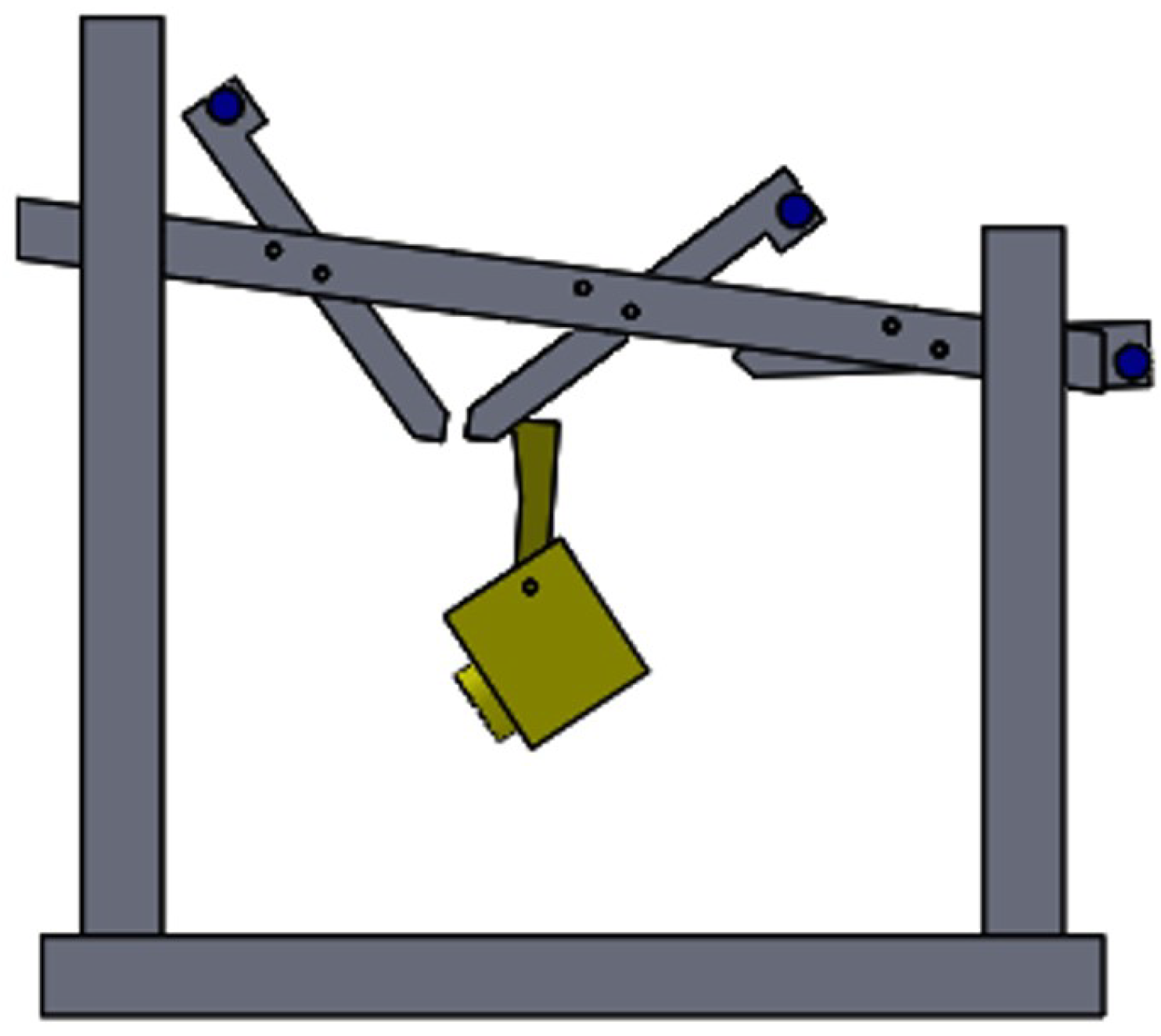
Figure 2. Aerial acrobat robot by Nishibori et al. [7].
Applsci 16 00921 g002
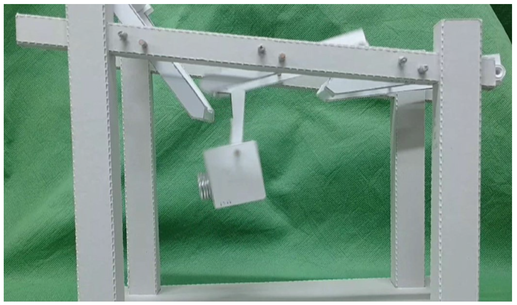
Figure 3. Top view of the structure of the paper craft aerial acrobatic robot prototype.
Applsci 16 00921 g003
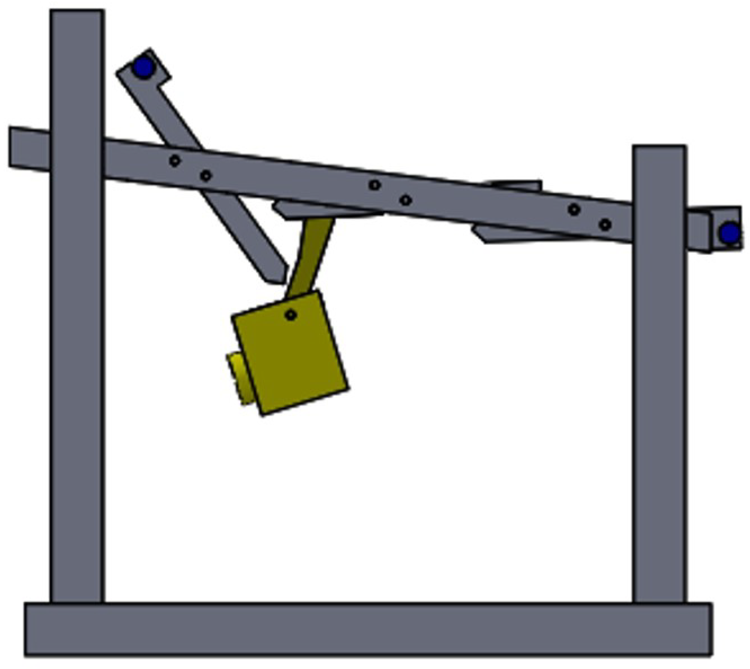
Figure 4. Oblique view of the structure of the paper craft aerial acrobatic robot prototype.
Applsci 16 00921 g004
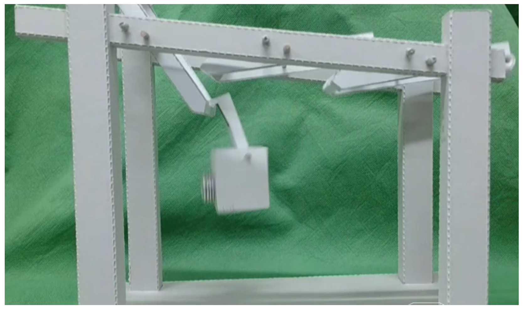
Figure 5. Side view of the structure of the paper craft aerial acrobatic robot prototype.
Applsci 16 00921 g005
Figure 6. Front view of the structure of the paper craft aerial acrobatic robot prototype.
Applsci 16 00921 g006
Figure 7. Top view of the structure of the paper craft aerial acrobat robot model.
Applsci 16 00921 g007
Figure 8. Oblique view of the structure of the paper craft aerial acrobat robot model.
Applsci 16 00921 g008
Figure 9. Oblique view of the paper craft robot prototype.
Applsci 16 00921 g009
Figure 10. Side view of the paper craft robot structure.
Applsci 16 00921 g010
Figure 11. Configuration of the aerial acrobatic robot and swing frames at time 0.0 s, illustrating the definition of angle  α  and the locations of shafts and counterbalances.
Applsci 16 00921 g011
Figure 12. State at  t = 0.3  s where the robot reaches the lowest point and the paper spring is fully deflected.
Applsci 16 00921 g012
Figure 13. Reduction of contact forces as the handrail tilts at time 0.57 s.
Applsci 16 00921 g013
Figure 14. The moment of detachment and subsequent free fall at time 0.61 s.
Applsci 16 00921 g014
Figure 15. Successful engagement with swing frame B and the beginning of the next rotation at time 0.62 s.
Applsci 16 00921 g015
Figure 16. Conceptual diagram of the swing frame based on the one-link model.
Applsci 16 00921 g016
Figure 17. Schematic of the two-link model employed for the Lagrangian formulation. Link lengths, joint angles, mass centers, and gravitational forces are defined for deriving the analytical equations of motion.
Applsci 16 00921 g017
Figure 18. Measurement of the torsional spring constant of the robot arm in its initial state, that is, without any added mass.
Applsci 16 00921 g018
Figure 19. Side view of robot in angles  α = 60  corresponding to Figure 18.
Applsci 16 00921 g019
Figure 20. Measurement of the torsional spring constant when the robot arm is tilted by the applied mass.
Applsci 16 00921 g020
Figure 21. Side view of robot in angles  α = 120  corresponding to Figure 20.
Applsci 16 00921 g021
Figure 22. Torsional spring constant  K T  of paper spring with respect to the angle change amount  Δ α .
Applsci 16 00921 g022
Figure 23. Paper surface combinations used for friction coefficient measurements: white surface-to-white surface, white surface-to-gray surface, and gray surface-to-gray surface.
Applsci 16 00921 g023
Figure 24. Measuring instrument of friction coefficient (INSTRON 5566) [25].
Applsci 16 00921 g024
Figure 25. Measurement of friction coefficient between paper surfaces based on the JIS K7125 friction test method (see friction test conditions in Table 2).
Applsci 16 00921 g025
Figure 26. Measurement results of friction coefficients between the white paper surface and the white paper surface.
Applsci 16 00921 g026
Figure 27. Measurement results of friction coefficients between the white paper surface and the gray paper surface.
Applsci 16 00921 g027
Figure 28. Measurement results of friction coefficients between the gray paper surface and the gray paper surface.
Applsci 16 00921 g028
Figure 29. Schematic diagram illustrating the applicability domains of the static model, dynamic two-link model, and multibody dynamics. The shaded regions indicate conditions where the underlying modeling assumptions are no longer valid.
Applsci 16 00921 g029
Figure 30. Operation of the robot prototype at time 0 s (where 0 s is defined as the moment when the robot’s arm engages with the swing frame).
Applsci 16 00921 g030
Figure 31. Operation of the robot model at time 0 s (where 0 s is defined as the moment when the robot’s arm engages with the swing frame).
Applsci 16 00921 g031
Figure 32. Operation of the robot prototype at time 0.3 s.
Applsci 16 00921 g032
Figure 33. Operation of the robot model at time 0.3 s.
Applsci 16 00921 g033
Figure 34. Operation of the robot prototype at time 0.4 s.
Applsci 16 00921 g034
Figure 35. Operation of the robot model at time 0.4 s.
Applsci 16 00921 g035
Figure 36. Operation of the robot prototype at time 0.57 s.
Applsci 16 00921 g036
Figure 37. Operation of the robot model at time 0.57 s.
Applsci 16 00921 g037
Figure 38. Operation of the robot prototype at time 0.62 s.
Applsci 16 00921 g038
Figure 39. Operation of the robot model at time 0.62 s.
Applsci 16 00921 g039
Figure 40. Time history of angles by measurements and multibody dynamics.
Applsci 16 00921 g040
Figure 41. Angles at each time point from a video recording of the paper craft aerial acrobat robot’s motion by using Kinovia.
Applsci 16 00921 g041
Figure 42. Angular velocities as functions of the swing frame angle obtained by measurements and multibody dynamics.
Applsci 16 00921 g042
Figure 43. Angular accelerations as functions of the swing frame angle obtained by theoretical analysis and multibody dynamics. (The raw data are available in the Supplementary Materials).
Applsci 16 00921 g043
Table 1. Representative lengths and masses in Figure 16 and Figure 17.
Mechanical PropertiesValue
Length  L a 0.0483 m
Length  L b 0.0517 m
Length  L c 0.03 m
Length  L d 0.06 m
Offset h0.005 m
Mass of the swing frame  m 1 0.0040 kg
Mass of the paper craft
Aerial acrobat robot model  m 2 0.00771 kg
Mass of counterbalance  m 3 0.00720 kg
Air density  ρ 1.29 kg/m3
Drag coefficient  C d 1.05 [19]
Table 2. Friction test conditions.
TemperatureHumidityVelocityForce
23 ± 2 °C50 ± 10%RH100 mm/min1.96 N
Table 3. Data of friction test.
Contact of Two ObjectsPeak
Force ( F S )
Average
Force ( F K )
Static Friction
Coefficient ( μ S )
Kinetic Friction
Coefficient ( μ K )
White surface/White surface0.993 N0.661 N0.5070.337
White surface/Gray surface1.063 N0.802 N0.5420.409
Gray surface/Gray surface0.556 N0.292 N0.2830.149
Table 4. Comparison of modeling approaches for the aerial acrobatic robot.
AspectQuasi-Static Single-Link Model (Nishibori Theory)Dynamic Two-Link ModelMultibody Dynamics (MBD)
Modeling conceptStatic torque balance of a single rigid linkAnalytical dynamic model of a two-link rigid-body systemGeneral multibody formulation with kinematic constraints
Degrees of freedomAngle  θ 1 Angles  θ 1 θ 2 Arbitrary (system-dependent)
Treatment of inertiaNot included in the original formulation; inertia introduced indirectly via  T = I θ ¨ 1 Explicitly included through Lagrange equationsFully included via mass and inertia matrices
Air dragNeglectedIncludedNeglected
Angular velocity effectsNeglectedIncludedIncluded
Angular accelerationEstimated indirectly from quasi-static torqueDirectly computed from equations of motionDirectly computed numerically
Gravity effectsIncludedIncludedIncluded
Friction modelingNeglectedNeglectedIncluded
Elastic elementsNot consideredNot consideredModeled as rotational spring elements of robot
Contact and temporal variabilityNot consideredNot consideredFully considered
Numerical methodNot requiredAnalytical ODEGSTIFF solver
Computational costVery lowLow to moderateHigh
Applicability domainQuasi-static motion with negligible inertia effect of robotLow-inertia two-link systemsGeneral multibody systems with contact and friction
LimitationsCannot represent sign reversal of angular accelerationsLimited to two-link configurationModel complexity and parameter identification
Disclaimer/Publisher’s Note: The statements, opinions and data contained in all publications are solely those of the individual author(s) and contributor(s) and not of MDPI and/or the editor(s). MDPI and/or the editor(s) disclaim responsibility for any injury to people or property resulting from any ideas, methods, instructions or products referred to in the content.