3.1. Experimental Design Rationale
We structure our experiments in two complementary phases to systematically address different aspects of the FL-IDS challenge, separating controlled component analysis from realistic cross-environment deployment conditions.
3.1.1. Phase 1: Attack-Only Classification (Single-Domain)
In our single-domain experiments (CICIDS-2017, InSDN-OVS, 5G-NIDD), we exclude benign traffic and focus exclusively on multiclass attack classification. This design choice is motivated by three factors:
Problem difficulty: In many settings, binary benign-vs-attack detection can reach very high performance due to clearer separability. The more challenging task is distinguishing between attack types, particularly rare classes such as BOTNET and Web-Attack.
Isolating class imbalance effects: By removing the dominant benign class (often exceeding 80% of traffic), we can more precisely evaluate how SMOTE placement, loss functions, and client selection affect inter-attack discrimination.
Ablation clarity: Attack-only settings provide cleaner ablation studies, allowing us to attribute performance changes directly to specific components (SMOTE, Focal Loss, rare-class-aware client selection).
3.1.2. Phase 2: Multi-Domain with Benign Traffic (Cross-Environment)
To evaluate cross-environment learning under a unified label space, we combine CICIDS-2017 and InSDN-OVS and include benign traffic to simulate realistic IDS deployment:
Operational realism: Production IDS must process predominantly benign traffic while detecting rare attacks. Including benign samples tests whether the model maintains low false positive rates, mitigating alert fatigue concerns.
Domain shift evaluation: Traffic patterns differ substantially across enterprise and SDN environments for both benign and attack classes. We observed that even identically named attacks, such as DDoS, show different feature distributions in CICIDS-2017 and InSDN-OVS, which can degrade detection performance. By including benign and attack samples from both sources, we test whether FL can learn more domain-robust representations under this cross-environment shift.
Threshold optimization: Our benign-gating mechanism (Equation (
2)) requires benign samples to tune the trade-off between attack recall and benign misclassification, which we quantify using the FP/10K metric.
This two-phase design enables both rigorous component attribution (Phase 1) and realistic cross-environment assessment (Phase 2). Crucially, success in inter-attack discrimination (Phase 1) implies a higher level of feature representation granularity; a model that can distinguish between subtly different attack vectors learns more robust decision boundaries than a simple binary classifier. This granular performance serves as a foundation for effective binary classification in broader deployment scenarios, as validated in Phase 2.
3.2. Common Experimental Settings
All experiments use SimpleMLP with two hidden layers [128, 64], BatchNorm1d, ReLU activation, and Dropout(0.3). We optimize with AdamW (lr =
, weight decay =
), batch size 256. Main experiments comparing Per-Client vs. Global SMOTE were repeated across 5 seeds (42, 123, 456, 789, 2024) to verify stability; see
Section 4.4 for aggregated statistics. Ablation studies use single-run results (seed = 42). To balance minority class representation without overfitting to synthetic samples, SMOTE is applied with a maximum 10:1 ratio, while this SimpleMLP serves as our base classifier, it is extended into an
MLPWithEncoder architecture in Phase 2 to incorporate representation learning, as detailed below.
3.2.1. Phase 1: Single-Domain Settings
We use stratified 70/15/15 train/validation/test splits per dataset. We use 5 FL clients, 15 communication rounds, 5 local epochs per round, with 3 clients selected per round. Rare attack classes are concentrated in two clients (0–1) to ensure sufficient neighborhood density for SMOTE synthesis. To ensure fair comparison, this distribution is maintained across all experimental variants. Each round includes at least one rare-enriched and one common client for balanced gradient updates. Focal Loss γ = 3.0. Feature counts: 28 for CICIDS/OVS, 43 for 5G-NIDD.
3.2.2. Phase 2: Multi-Domain Settings
Each source dataset (CICIDS, OVS) is first split 70/15/15 into train/validation/test. The test and validation portions are combined into global pools: the global test set is held out for final evaluation, while the global validation set is reserved for threshold optimization (
Section 3.5.5). The combined training pool undergoes a nested split: 90/10 for AE pretraining (AE-train/AE-val), with the AE-train further divided 70/30 for federated training and round-end validation (FT-train/FT-val). We use 10 clients, 10 rounds, and 2 local epochs with full client participation (
Table 3).
For representation learning, we employ a Denoising AutoEncoder (DAE) with a 32-dimensional latent space (see
Section 3.5.3 for architecture and justification). Pretraining is fully unsupervised; labels are introduced only during federated fine-tuning.
3.3. Summary of Experimental Hyperparameters
To provide a unified reference,
Table 3 summarizes key configurations for both experimental phases.
While non-IID conditions typically motivate advanced aggregation methods, FedAvg proves sufficient in our framework due to a dual-layer mitigation strategy: (1) DAE pretraining (37 → 256 → 128 → 64 → 32) provides a shared, domain-invariant initialization that filters environment-specific noise and reduces gradient divergence, and (2) Per-Client SMOTE addresses label skew locally before training. This combination ensures stable convergence and high-stakes detection performance without the computational overhead of constrained optimization algorithms.
3.4. Domain-Specific FL Pipeline
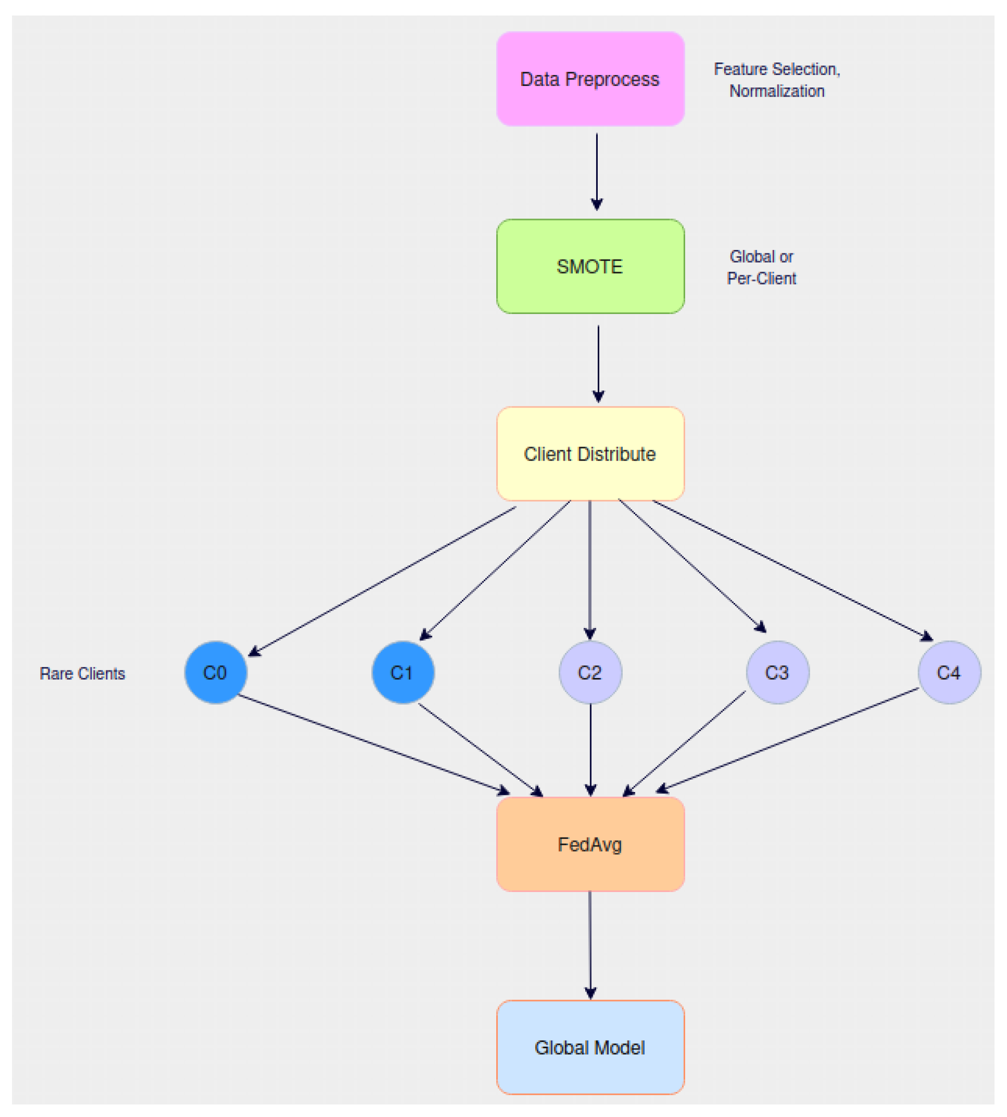
Figure 1 illustrates the domain-specific FL pipeline, which consists of four stages:
Data Preprocessing: We apply dataset-specific cleaning and harmonization (e.g., rate-column fixes, label text normalization), followed by feature selection and StandardScaler normalization fitted only on the training split. We then create a stratified train/validation/test split (70%/15%/15%). In Phase 1 single-domain settings, benign samples are excluded to focus on inter-attack discrimination.
To prevent data leakage, all preprocessing statistics (feature selection scores and StandardScaler) are computed using only the training split. Likewise, all balancing steps (Global/Per-Client SMOTE) are applied only to the training data; validation and test sets remain untouched.
SMOTE Application: We compare two oversampling placements: (i) Global SMOTE applied before client distribution, and (ii) Per-Client SMOTE applied independently after distribution. We adopt an adaptive neighbor rule , targeting the median class, count as a cap to avoid excessive synthesis under extreme rarity.
Client Distribution: Data are distributed across 5 clients following the rare-concentrated allocation in
Table 3, simulating non-IID deployments where only a subset of sites observe rare attacks.
Federated Training: FedAvg and early stopping settings follow
Table 3. Rare-aware selection ensures balanced gradient updates from both rare-enriched and common clients each round.
Dataset-Specific Notes
CICIDS-2017: We perform MI-based feature selection to obtain 28 features. Rate-related columns (e.g., Flow_Bytes/s, Flow_Packets/s) are corrected, values are clipped at the 99.9th percentile, and missing values are imputed using medians computed from the CICIDS training split. The six attack classes include {BFA, BOTNET, DDoS, DoS, Probe, Web-Attack}, where BFA, BOTNET, and Web-Attack are treated as rare.
InSDN-OVS: We use the same 28-feature MI-based selection to maintain comparability. We fix label formatting artifacts (e.g., trailing whitespace in DDoS labels) and impute missing values using medians from the OVS training split. Because rare classes are more sparse in OVS, we use stronger class-wise weights in Focal Loss compared to CICIDS.
5G-NIDD: We remove the benign class and perform one-hot encoding on categorical attributes (e.g., Proto, State, Cause). Columns with more than 70% missing values are dropped. StandardScaler is fitted on the training split after encoding and applied to validation/test. The eight attack classes include {HTTPFlood, ICMPFlood, SYNFlood, SYNScan, SlowrateDoS, TCPConnectScan, UDPFlood, UDPScan}, with ICMPFlood and SYNFlood treated as rare.
3.5. Multi-Domain FL Pipeline
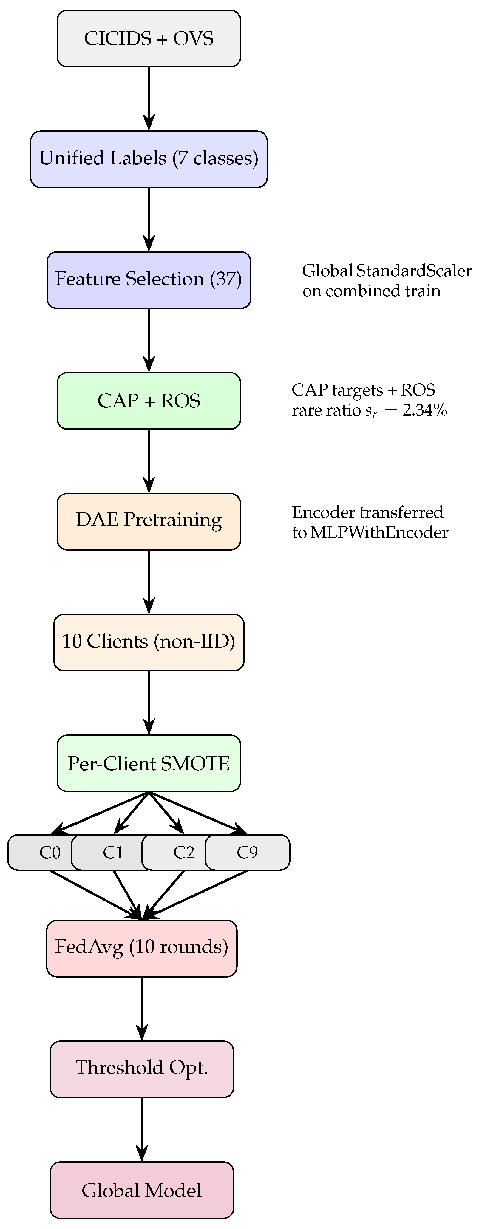
To examine cross-environment learning under a unified label space, we combine CICIDS-2017 and InSDN-OVS into a 7-class problem: {BENIGN, BFA, BOTNET, DDoS, DoS, Probe, Web-Attack}. We exclude U2R because it appears only in CICIDS-2017 and is extremely scarce (<50 samples), which makes learning unstable and evaluation unreliable. Beyond sample scarcity, the high intraclass variance of U2R exploits (e.g., buffer overflows and rootkits) cannot be effectively captured by such a limited sample size, particularly in a federated setting where data are further partitioned across clients. Including U2R would lead to results dominated by statistical noise rather than genuine feature representation. Thus, removing U2R ensures a more robust label space for cross-domain evaluation and avoids conclusions driven by near-zero support.
Figure 2 summarizes the end-to-end multi-domain FL pipeline.
To prevent data leakage, we adopt the nested split strategy detailed in
Section 3.2 (Phase 2 settings). All resampling is applied exclusively to FT-train; validation and test splits remain untouched.
3.5.1. Feature Harmonization and Selection
We align the datasets using a common feature schema, facilitated by the fact that both CICIDS-2017 and InSDN-OVS were generated using the same extraction tool (CICFlowMeter). This ensures that features such as Flow_Duration and Packet_Length carry identical semantic and technical definitions across both environments, providing a consistent baseline for harmonization. We then apply a correlation filter (threshold 0.90), followed by mutual information ranking to select the top 37 features. This selection process focuses on protocol-standard flow characteristics (e.g., packet counts, duration, and byte rates) that are semantically consistent across different network environments. By prioritizing these domain-agnostic features and utilizing a shared extraction methodology, we minimize the risk of environmental bias being encoded into the harmonized feature space.
3.5.2. Client Setup and FL Configuration
Unlike the single-domain experiments, the multi-domain setting uses 10 clients. All clients participate in each round, with 10 rounds total and 2 local epochs per round. We use full participation to make aggregation more stable under cross-domain label sparsity.
3.5.3. AutoEncoder Pretraining
To mitigate cross-domain feature mismatch, we use a Denoising AutoEncoder (DAE) for representation learning. The encoder maps
to a latent space
:
The compression ratio (
) provides a meaningful bottleneck that prevents identity mapping and forces the encoder to filter environment-specific noise, essential for cross-domain alignment. The decoder mirrors this structure to reconstruct
by minimizing MSE loss. We inject Gaussian noise with
during pretraining to improve robustness. This pretraining phase is fully unsupervised; no class labels are used.
We pretrain the DAE on the aggregated multi-domain training pool (CICIDS + OVS) to obtain a shared initialization. The pretrained encoder is then used to initialize each client model in MLPWithEncoder. During federated training, the encoder and classifier are optimized jointly on each client (no freezing) under the same Per-Client SMOTE protocol, and updates are aggregated via FedAvg.
To isolate the contribution of representation pretraining, both AE-based and Pure MLP baselines use the same federated optimization protocol and the same Per-Client SMOTE strategy. The only difference is DAE initialization.
Computational Overhead
While DAE pretraining introduces a one-time computational cost (12 epochs with early stopping on the combined training pool), this overhead is negligible compared to the long-term benefits: (1) faster and more stable FL convergence through domain-invariant initialization (see
Section 3.3 for FedAvg justification), (2) a modest reduction in the classifier’s input dimensionality during fine-tuning (32 vs. 37), which can slightly lower the computational cost of the classification head and simplify optimization, and (3) significantly improved cross-domain generalization. The pretraining cost is amortized across all subsequent FL experiments using the same dataset combination, and it serves as a critical trade-off for achieving a 0.7739 Global Macro-F1 score in multi-domain settings.
3.5.4. Hierarchical Balancing: CAP, ROS, and Per-Client SMOTE
To address extreme class imbalance in the combined multi-domain distribution, we apply a three-tier hierarchical balancing strategy that operates sequentially at both global and local levels:
CAP (Global-level): Mitigates major-class dominance by applying hard limits to high-frequency traffic: BENIGN K, DoS K, DDoS K, and Probe K. Rare classes remain untouched, allowing the optimizer to capture diverse attack gradients without being overwhelmed by the majority.
Conservative ROS (Global-level): Acts as a bootstrapping seed for rare classes (BFA, BOTNET, and Web-Attack). By applying a cap per rare class (adding approximately 154 samples each), we achieve an aggregate rare-class ratio of . This step is technically critical; it ensures a sufficient “starting population” so that local clients receive enough samples () after partitioning to make subsequent SMOTE interpolation viable.
Per-Client SMOTE (Client-level): Addresses the residual scarcity that emerges after StratifiedKFold distribution across 10 clients. For example, while the BOTNET count drops to ∼108 samples per client after partitioning, Per-Client SMOTE restores this to a target of 500 (a local increase). For extremely scarce classes such as Web-Attack, we apply a more conservative target of 150 samples to prevent overfitting on synthetic noise while still providing sufficient diversity for the model.
This sequential pipeline, applying CAP+ROS globally and SMOTE locally with an adaptive neighbor rule, prevents global balancing gains from being diluted by the federated partitioning process. The effectiveness of this interaction is validated by our results, where previously undetected classes such as BOTNET achieved a Macro-F1 score of 0.5744. To maintain the integrity of the evaluation, all balancing steps are applied exclusively to the training split.
3.5.5. Threshold Optimization
For multi-domain inference, we use a benign gate followed by class-specific constraints. Let
denote rare classes,
denote major attack classes, and
. Given predicted probabilities
, we define
and
.
where
is the benign gating threshold,
are per-class thresholds for major attack classes, and
are rare-class confidence and margin constraints.
If no attack class meets the constraints above, the prediction defaults to BENIGN. Thresholds are optimized on the validation set using grid search with a step size of 0.005 (yielding 57 candidate values for ) to maximize Macro-F1 while keeping false positives at ≤500 per 10K benign samples. Convergence was verified by comparing quantile-based and grid-based optimization, both yielding identical per-class thresholds.
3.6. Experiment Matrix
To ensure reproducibility and isolate the effect of imbalance handling from federated aggregation, we define an experiment matrix spanning SMOTE placement, loss choice, and client-selection variants across three single-domain datasets and one multi-domain setting. We run the full ablation suite on CICIDS-2017 as the primary benchmark. For InSDN-OVS and 5G-NIDD, we report a smaller set of representative configurations (full pipeline, Per-Client SMOTE variant, and a centralized baseline). This design checks whether key findings generalize across datasets without making the experiment grid too large.