Evidence-Weighted Multi-Criteria Decision Support for Subjective Quality Assessment Under Sparse and Unbalanced Information

Abstract

Decision making for complex products often depends on subjective user experience, while competing alternatives may be supported by strongly unequal numbers of observations. This study develops an evidence-weighted multi-criteria decision-making methodology for such sparse and unbalanced information. A seven-category rating scale is aggregated at the respondent level and transformed affinely to [0, 1]. Domain-specific variance components are estimated by restricted maximum likelihood and used for empirical Bayes partial pooling, so that sparse estimates are moderated without excluding valid alternatives. AHP preference weights are kept conceptually separate from evidence weights, inherent product quality is separated from non-inherent ownership attributes, and uncertainty is propagated through Monte Carlo simulation. The empirical demonstration comprised 140 unique questionnaire records for 21 agricultural tractor brands with sample sizes from 1 to 50. Compared with direct averaging, the empirical Bayes ranking was highly preserved (Spearman $\rho =0.992$) while unsupported extremes were reduced. A controlled simulation showed lower RMSE for empirical Bayes than for the arithmetic mean, median, and fixed shrinkage under both Gaussian and bounded non-Gaussian data generation, with the largest benefit at $n=1$. Sensitivity analyses showed high ranking stability to the upper-level quality weight, perturbations of AHP weights, and bounded score transformations. The framework therefore provides reproducible uncertainty-aware decision support without treating weak evidence as either absent or equally strong as data-rich evidence.

1. Introduction

Decision making in engineering and product selection rarely depends exclusively on characteristics that can be measured directly in physical units. Parameters such as mass, power, torque, dimensions, capacity, and fuel consumption can generally be compared objectively once measurement procedures and units are standardized. A more difficult problem arises when decision-relevant characteristics are expressed primarily through user experience rather than through a natural physical metric.

Perceived usability, operator comfort, accessibility of controls, practical maintainability, workmanship, experienced reliability, service availability, and ownership satisfaction are examples of attributes that may strongly influence real decisions but necessarily contain a subjective component. Their quantification requires both a defensible measurement system and a method for representing unequal strength of evidence.

The resulting problem belongs naturally to operations research (OR) and multi-criteria decision making (MCDM), where a finite set of alternatives is evaluated under heterogeneous criteria, preference structures, incomplete information, and uncertainty [1,2,3,4]. Classical MCDM established formal structures for weighting and ranking alternatives, with AHP providing a widely used mechanism for eliciting criterion importance through pairwise comparisons [1,2]. More recent work has increasingly emphasized transparent and uncertainty-aware decision support, including fuzzy MCDM architectures and reliability- and risk-oriented engineering applications [5,6]. In parallel, statistical hierarchical models, empirical Bayes shrinkage, and small-area estimation have developed methods for stabilizing estimates supported by unequal sample sizes [7,8,9,10,11,12]. These two methodological streams address different parts of the same decision problem but are still commonly applied separately.

The present work continues an earlier methodological research line in which overall machine quality was treated as a synthetic property derived from partial quality characteristics rather than as a directly measurable physical quantity [13]. Related work demonstrated how quantitative machine assessment can support machinery selection decisions using structured user-derived information [14].

A fundamental conceptual distinction is made between inherent and non-inherent attributes. Inherent characteristics belong to the product itself. Price, spare parts availability, service accessibility, and similar ownership environment characteristics influence the decision but are not physical properties of the product. Keeping these dimensions separate prevents favorable market support from being misinterpreted as inherent technical quality.

The proposed framework deliberately concentrates on subjectively assessed characteristics. Directly measurable variables may be added to a broader decision model, but they do not create the same inferential problem because their values can be compared directly after standardization. The unresolved methodological gap addressed here is the conversion of subjective ratings into quantitative alternative-level information when the number of observations differs strongly among alternatives, while simultaneously preserving a transparent preference structure and explicitly propagating uncertainty.

A direct arithmetic mean ignores differences in evidence strength. An alternative represented by one observation and one represented by fifty observations may receive similar point estimates despite radically different uncertainty. Conversely, a hard eligibility threshold protects against sparse extremes only by discarding otherwise valid alternatives. The key question is therefore not whether sparse evidence should be accepted or rejected, but how strongly it should influence an alternative-specific estimate.

The proposed solution separates two types of weighting that are frequently conflated. AHP weights represent decision preference: how important is a quality domain? Empirical Bayes weights represent evidence strength: how much should the observed result for a particular alternative influence its estimate? The first is an MCDM preference problem; the second is a hierarchical inference problem.

A further requirement concerns the measurement scale itself. Statistical sophistication cannot compensate for an incoherent source scale. The proposed framework therefore begins with a seven-category ordered rating scale, treats consecutive categories as equally spaced for respondent-level aggregation, preserves the finite end points through affine normalization, and derives interpretation classes from the same numerical geometry. This design is informed by classical work on rating scales and by evidence that appropriately treated Likert-type data can support parametric summaries when the analytical assumptions and purpose are made explicit [15,16].

The novelty of this study does not reside in AHP, REML, empirical Bayes, geometric aggregation, or Monte Carlo simulation individually. It lies in a functional architecture in which (I) respondent-level measurement is separated from between-alternative inference, (II) evidence strength is estimated from the observed variance structure rather than imposed through a sample-size threshold, (III) evidence weights are kept distinct from AHP preference weights, (IV) inherent and non-inherent attributes remain diagnostically separate until final synthesis, and (V) uncertainty is propagated to probabilistic rankings. The revised study additionally validates this architecture through an empirical benchmark, a controlled simulation with known truth, and preference/distributional sensitivity analyses.

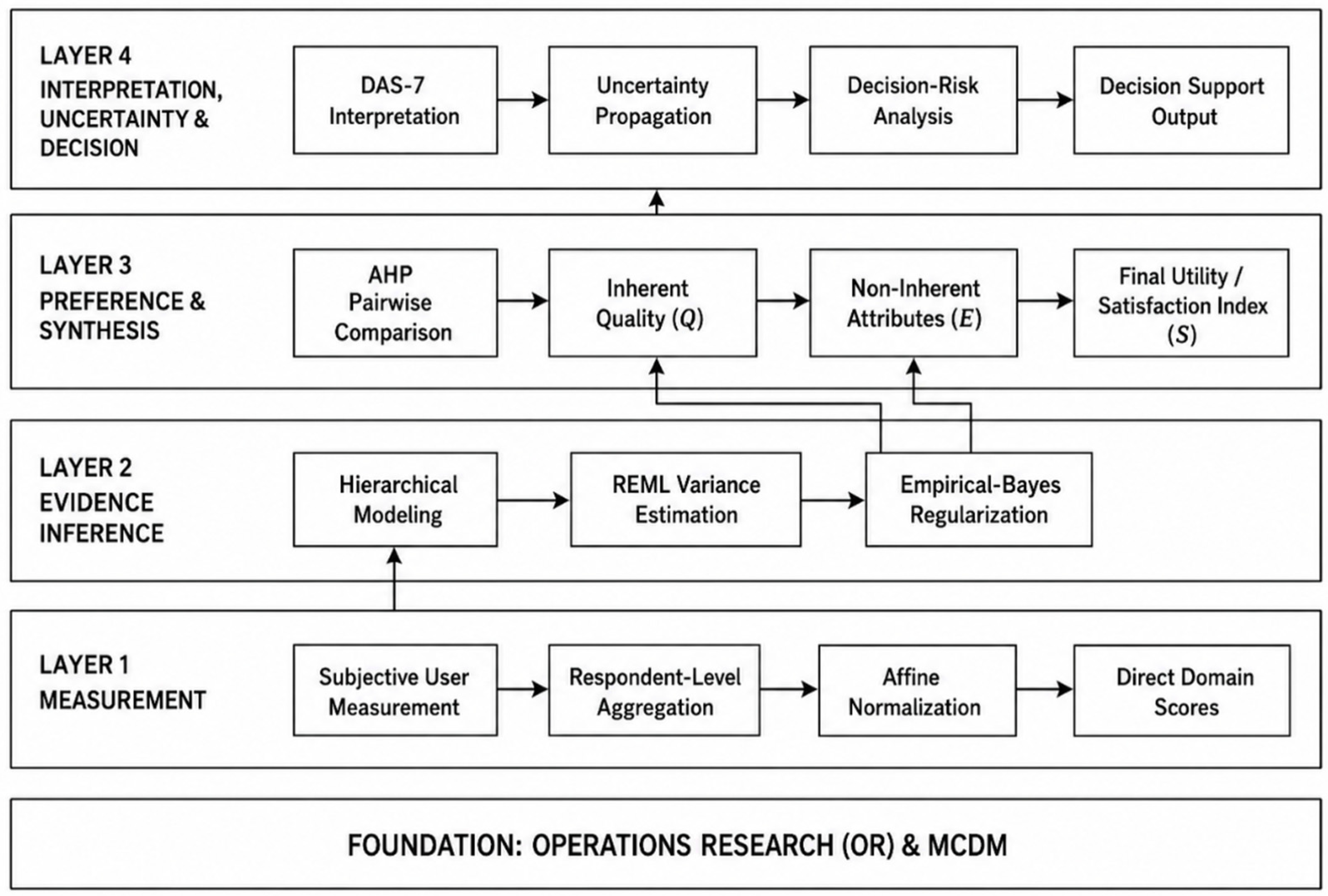
The overall logic of the proposed evidence-weighted MCDM framework is summarized in Figure 1, which shows the sequential integration of subjective measurement, evidence inference, preference modeling, multi-criteria synthesis, and uncertainty-aware decision support within an operations research structure.

The research objective was to develop and quantitatively validate a reproducible methodology capable of retaining even single valid observations without treating them as equivalent to large samples, separating preference weights from evidence weights, distinguishing inherent quality from non-inherent decision attributes, and propagating uncertainty to the final decision support stage. The remainder of the paper is organized as follows. Section 2 defines the measurement, hierarchical estimation, MCDM synthesis, benchmark, simulation, and sensitivity procedures; Section 3 reports the empirical and simulation results; Section 4 discusses methodological implications, robustness, and limitations; and Section 5 summarizes the principal conclusions.

2. Materials and Methods

2.1. Decision Structure

Let the finite set of decision alternatives be denoted by $\mathcal{A}$ and the set of subjectively evaluated criteria by $\mathcal{C}$. The decision problem is represented by the alternatives, criteria, preference structure $\mathit{W}$, empirical evidence $\mathcal{E}$, and uncertainty $\mathcal{U}$:

$$\mathcal{D}=\left(\mathcal{A},\mathcal{C},\mathbf{W},\mathcal{E},\mathcal{U}\right)$$

(1)

The core inferential component is intended for attributes whose practically relevant values are elicited through structured judgment rather than direct physical measurement.

Index convention: $i$ = respondent; $j$ = alternative; $k$ = detailed criterion; $g$ = assessment domain; $r$ and $s$ = AHP domain indices; $\mathcal{l}$ = DAS-7 level; $b$ = Monte Carlo realization. Uppercase $C$, $H$, $O$, $R$, $Q$, $E$ and $S$ denote domain or aggregate scores. Calligraphic symbols denote sets or information structures.

2.2. Subjective Measurement and Respondent-Level Aggregation

Respondent $i$ evaluates alternative $j$ on criterion $k$ using the common seven-category scale:

$$x_{ijk}\in \{1,2,\dots ,7\}$$

(2)

The questionnaire used a common seven-category ordered scale for all detailed criteria. The original instrument explicitly defined category 1 as an unacceptable level and category 7 as an outstandingly good level; integers 2–6 represented ordered intermediate judgments. Category 4 is therefore treated as the numerical midpoint of the scale rather than as an independently validated semantic neutral anchor. All criteria were oriented in the same direction, with higher values representing more favorable states, so no reverse coding was required. The final questionnaire contained 44 detailed criteria assigned a priori to five non-overlapping domains: Cabin (15 items), Handling and Usability (12), Operation (8), Reliability (5), and non-inherent ownership-related attributes (4). The domain structure followed the functional architecture of the AGRORANKING questionnaire; criteria were allocated according to their primary engineering or operational meaning, and no criterion was assigned to more than one domain. Because no separate external content validity study was conducted, completeness of the criterion family is treated as an application-specific limitation rather than a universal claim. Within domain $g$, detailed responses are aggregated before inferential modeling:

$${\overline{x}}_{ijg}={\displaystyle \frac{1}{m_{ijg}}}\sum _{k\in g}{x}_{ijk}$$

(3)

where $m_{ijg}$ is the number of valid item responses for respondent $i$, alternative $j$, and domain $g$. The respondent record, not the individual questionnaire item, is the statistical unit, preventing item-level pseudoreplication. In the final analyzed dataset, all 140 records contained complete ratings for all 44 detailed criteria; the general $m_{ijg}$ formulation is retained so that the method remains applicable to future datasets containing item-level missingness.

2.3. Affine Normalization

Respondent domain scores are mapped to the unit interval as:

$$z_{ijg}={\displaystyle \frac{{\overline{x}}_{ijg}-1}{6}}$$

(4)

The mapping preserves the finite scale anchors exactly: 1 maps to 0, 4 maps to 0.5, and 7 maps to 1. It therefore introduces no additional nonlinear utility assumption.

2.4. Direct Alternative Estimate

After affine normalization, the direct score for alternative $j$ within domain $g$ was calculated as the arithmetic mean of the normalized respondent-level observations:

$${\overline{z}}_{jg}={\displaystyle \frac{1}{n_{jg}}}{\displaystyle {\sum }_{i=1}^{n_{jg}}}{z}_{ijg}$$

(5)

where $n_{jg}$ is the number of respondent records contributing valid information to alternative $j$ in domain $g$. The arithmetic mean preserves numerical discrimination but does not account for differences in evidence strength.

2.5. Hierarchical Random Effects Model and REML

For each domain, respondent-level observations are modelled as:

$$z_{ijg}={\mu }_g+u_{jg}+{\epsilon }_{ijg}$$

(6)

$$u_{jg}\sim \mathcal{N}\left(0,{\tau }_g^2\right),\hspace{1em}{\epsilon }_{ijg}\sim \mathcal{N}\left(0,{\sigma }_g^2\right)$$

(7)

The latent state for alternative $j$ in domain $g$ is denoted ${\theta }_{jg}$. The domain-specific variance components are denoted ${\tau }_g^2$ and ${\sigma }_g^2$ and are estimated using restricted maximum likelihood (REML), a standard approach to variance-component estimation in unbalanced mixed models [7,8].

Formally, the latent alternative state is the sum of the domain-specific population mean and the alternative-specific random deviation:

$${\theta }_{jg}={\mu }_g+u_{jg}$$

The between-alternative variance quantifies heterogeneity of latent alternative states within a domain, whereas the within-alternative variance quantifies record-level dispersion around those states. Observed normalized responses are bounded to [0, 1]; the Gaussian random effects and residual terms are working latent variables and are not hard-bounded.

2.6. Empirical Evidence Weight and Empirical Bayes Estimate

Conditional on the fitted variance components, the empirical evidence weight is:

$$B_{jg}={\displaystyle \frac{{\widehat{\tau }}_g^2}{{\widehat{\tau }}_g^2+{\widehat{\sigma }}_g^2/n_{jg}}}={\displaystyle \frac{n_{jg}}{n_{jg}+v_g}},\hspace{1em}{v}_g={\displaystyle \frac{{\widehat{\sigma }}_g^2}{{\widehat{\tau }}_g^2}}$$

(8)

The quantity $B_{jg}$ is termed the Empirical Evidence Weight (EEW). It is not a probability of truth or a percentage of credibility; it represents the model-based share of alternative-specific evidence in the regularized estimate. The empirical Bayes estimator is:

The dimensionless ratio appearing in Equation (8) equals within-alternative variance divided by between-alternative variance. At fixed sample size, a larger ratio implies stronger empirical Bayes shrinkage toward the domain mean, whereas a smaller ratio yields an evidence weight closer to one and preserves more of the direct alternative mean. Hats denote REML plug-in estimates.

$${\tilde{z}}_{jg}={\widehat{\mu }}_g+B_{jg}\left({\overline{z}}_{jg}-{\widehat{\mu }}_g\right)=B_{jg}{\overline{z}}_{jg}+\left(1-B_{jg}\right){\widehat{\mu }}_g$$

(9)

As $n_{jg}$ increases, $B_{jg}$ approaches one and the empirical Bayes estimate approaches the direct mean. Sparse estimates borrow more strength from the population of comparable alternatives. The approach is related to empirical Bayes and small-area estimation concepts developed in the James–Stein and Fay–Herriot traditions [9,10,11,12].

2.7. AHP Pairwise Comparison Weighting of Inherent Quality Domains

Preference importance is estimated independently from evidence strength. The empirical application contained four inherent domains: Cabin ($C$), Handling and Usability ($H$), Operation ($O$), and Reliability ($R$). The pairwise comparison judgments used to construct the reciprocal AHP matrix were provided by the editorial team of top agrar Polska, which operates the AGRORANKING.pl portal. Saaty’s fundamental scale was used for the comparisons [1,2]:

$$\mathbf{A}=\left[a_{rs}\right],\hspace{1em}{a}_{sr}={\displaystyle \frac{1}{a_{rs}}},\hspace{1em}{a}_{rr}=1$$

(10)

The priority vector w was obtained from the principal eigenvector of A:

$$\mathbf{A}\mathbf{w}={\lambda }_{\mathrm{m}\mathrm{a}\mathrm{x}}\mathbf{w},\hspace{1em}{\displaystyle {\sum }_{r=1}^p}{w}_r=1$$

(11)

The resulting elicited matrix produced ${\lambda }_{\mathrm{m}\mathrm{a}\mathrm{x}}=4.2489$, $\mathrm{C}\mathrm{I}=0.0830$, and $\mathrm{C}\mathrm{R}=0.0922$. Because $\mathrm{C}\mathrm{R}<0.10$, the internal consistency of the pairwise judgments was considered acceptable. The normalized eigenvector weights, ordered as $C$, $H$, $O$, and $R$, were 0.0834, 0.2321, 0.1347, and 0.5499, respectively. The normalized weights and consistency diagnostics are reported above, and the computational settings are included in the Supplementary Materials. The complete pairwise comparison matrix, together with the priority vector and full consistency calculations, is provided in Supplementary Table S4.

2.8. Inherent Quality and Non-Inherent Attributes

The empirical Bayes-adjusted domain scores for alternative $j$ are denoted $C_j$, $H_j$, $O_j$, and $R_j$. Overall inherent quality is:

$$Q_j=0.0834C_j+0.2321H_j+0.1347O_j+0.5499R_j$$

(12)

Non-inherent decision attributes are retained separately and represented by the score $E_j$. In the AGRORANKING application, the $E$ domain comprised price-to-quality perception, spare parts availability, authorized service availability, and satisfaction with service support.

2.9. Final Multi-Criteria Utility Synthesis

The upper-level dimensions are combined through a weighted geometric function:

$$S_j=Q_j^{\alpha }{E}_j^{1-\alpha },\hspace{1em}0<\alpha <1$$

(13)

For the empirical application $\alpha =0.75$ was used as an explicit decision preference parameter assigning greater importance to inherent product quality. It was not estimated from the response data. The geometric form reduces, but does not eliminate, compensation between technical quality and ownership environment conditions; sensitivity to $\alpha$ is evaluated separately in Section 2.16. The value was based on an expert judgment provided by the editorial team of top agrar Polska: inherent product quality was assessed as three times as important as the external attributes dimension, corresponding to normalized upper-level weights of 0.75 and 0.25, respectively.

2.10. DAS-7 Measurement-Consistent Interpretation

After Equation (4), the seven source anchors occur at 0, 1/6, 2/6, 3/6, 4/6, 5/6, and 1. The DAS-7 class index is denoted by $\mathcal{l}$, and class boundaries are defined as the midpoints between consecutive anchors:

$$d_{\mathcal{l}}={\displaystyle \frac{2\mathcal{l}-1}{12}},\hspace{1em}\mathcal{l}=1,\dots ,6$$

(14)

This gives 0.0833, 0.2500, 0.4167, 0.5833, 0.7500, and 0.9167 and defines the Durczak Seven-Level Scale (DAS-7).

The measurement-consistent interpretation of the normalized scores is provided by the DAS-7 system, whose seven classes and corresponding semantic meanings are summarized in

Table 1. DAS-7 interpretation system.

Final Satisfaction	Non-Inherent Attributes	Inherent Quality	Interval	Level
extremely low	extremely unfavorable	critical	[0, 0.0833)	1
very low	very unfavorable	very low	[0.0833, 0.2500)	2
low	unfavorable	low	[0.2500, 0.4167)	3
moderate	moderate	moderate	[0.4167, 0.5833)	4
high	favorable	good	[0.5833, 0.7500)	5
very high	very favorable	very good	[0.7500, 0.9167)	6
exceptionally high	exceptionally favorable	excellent	[0.9167, 1.0000]	7

.

2.11. Model-Based Uncertainty and Probabilistic Ranking

Conditional on the REML-estimated variance components, the model-based variance of the empirical Bayes alternative domain estimate is:

$$V_{jg}={\displaystyle \frac{{\widehat{\tau }}_g^2{\widehat{\sigma }}_g^2}{n_{jg}{\widehat{\tau }}_g^2+{\widehat{\sigma }}_g^2}}$$

(15)

For each alternative $j$ and domain $g$, 20,000 Monte Carlo realizations were generated from a Gaussian distribution centered at the empirical Bayes estimate with the model-based variance $V_{jg}$. Simulated values below 0 or above 1 were clipped to the nearest admissible boundary. For each realization $b$, $Q$, $E$, and $S$ were recalculated. For two alternatives $j$ and $j^{\prime }$, pairwise superiority is defined as:

The uncertainty propagation is conditional on the REML plug-in estimates of the domain mean and the two variance components. Estimation uncertainty in these hyperparameters is not propagated in the present Monte Carlo analysis; the reported intervals and rank probabilities should therefore be interpreted as conditional model-based uncertainty rather than full parameter uncertainty.

The five domain-specific hierarchical models are fitted separately, and Monte Carlo realizations are generated independently across domains conditional on their marginal fitted models. This factorization is a modeling simplification, not an empirical claim of cross-domain independence. Across the 140 unique questionnaire records, Pearson correlations among the normalized domain scores ranged from 0.682 to 0.875 (Supplementary Table S5). Because all upper-level aggregation weights are positive, omitting positive cross-domain covariance can understate the variance of the weighted inherent quality aggregate and may narrow the uncertainty propagated to the final score and its rank probabilities. A multivariate hierarchical extension that jointly models cross-domain covariance is therefore an important direction for future work.

$$z_{jg}^{\left(b\right)}\sim \mathrm{N}({\tilde{z}}_{jg}, V_{jg})$$

$$p_{j{j}^{\prime }}=P \left(S_j>S_{j^{\prime }}\mid \mathcal{E}\right)$$

(16)

Rank probabilities were estimated from the simulated ranking distribution. This distinguishes uncertainty about the alternative state from the deterministic ordering of point estimates. Decision selection risk can additionally be summarized through expected opportunity loss, although the empirical demonstration focuses primarily on uncertainty and rank probabilities [3,6,12].

2.12. AGRORANKING Empirical Demonstration

AGRORANKING is the structured evidence acquisition system used to demonstrate the methodology. The final empirical dataset contained 140 unique questionnaire records covering 21 agricultural tractor brands, with sample sizes ranging from 1 to 50 records per brand. Each record referred to one tractor, and therefore one brand, and the same record supplied assessments across all five domains. Each record had a unique response identifier. Because the survey data used for analysis were anonymized, respondent identity across separate submissions could not be independently verified; independence between records is therefore a working assumption of the empirical model. All 44 detailed ratings were complete in the final analyzed dataset. The tractor application should be interpreted as a demanding real-world demonstration of sparse and strongly unbalanced evidence, not as a causal estimate of intrinsic brand effects. Accordingly, the term “unique questionnaire records” is used throughout the manuscript; empirical independence of respondents across separate submissions is not claimed.

2.13. Computational Reproducibility and AI-Assisted Preparation

The computational workflow was organized as a reproducible sequence of respondent-level aggregation, REML estimation, empirical Bayes regularization, AHP weighting, final utility synthesis, Monte Carlo uncertainty propagation, empirical benchmarking, controlled simulation, and sensitivity analysis. An anonymized respondent-level dataset and executable computational code are included with the revised submission to permit independent reproduction of the numerical results. During manuscript preparation, OpenAI ChatGPT was used to assist with manuscript structuring, language editing, mathematical notation checking, and computational verification. The author reviewed and verified the methodological assumptions, numerical outputs, interpretations, and final scientific content and takes full responsibility for the work. The AI-assisted preparation used ChatGPT (OpenAI, San Francisco, CA, USA). The specific ChatGPT software/model version used during manuscript preparation was not recorded and is therefore not stated retrospectively.

2.14. Comparative Benchmark Against Simpler Aggregation Strategies

To quantify the practical consequences of evidence weighting, the empirical Bayes procedure was benchmarked on the same 140 records against four simpler strategies: direct arithmetic mean aggregation, median aggregation, a hard minimum sample rule retaining only alternatives with $n_j\ge 3$, and a fixed-target shrinkage estimator. The downstream AHP weights, $Q/E$ separation, and geometric synthesis were kept unchanged so that only the evidence aggregation rule differed between methods.

The fixed-target benchmark shrank each direct domain mean toward the corresponding pooled domain mean using a sample-size-only coefficient $B_j^{\mathrm{F}}={\displaystyle \frac{n_j}{\left(n_j+3\right)}}$. Unlike the proposed empirical Bayes coefficient, this benchmark does not adapt to the estimated ratio of within-domain to between-alternative variability.

Rankings were compared with the empirical Bayes ranking using Spearman and Kendall rank correlations, mean absolute rank shift, maximum absolute rank shift, and the standard deviation of the final score $S$. For the $n_j\ge 3$ threshold strategy, the number and proportion of excluded alternatives were additionally recorded.

2.15. Controlled Simulation Study

To evaluate performance when the true alternative-level quality was known, a controlled Monte Carlo simulation reproduced the empirical structure of 21 alternatives and five domains. The observed sample-size pattern was preserved exactly: 50, 18, 15, 12, 8, 5, 4, 4, 3, 3, 3, 2, 2, 2, 2, 2, 1, 1, 1, 1, and 1 observations per alternative. Domain-specific location and variance scales were calibrated to the REML estimates obtained from the empirical data.

Scenario $A$ represented a correctly specified Gaussian random effects hierarchy. For each domain $g$, true alternative quality was generated as ${\theta }_{jg}={\mu }_g+u_{jg}$ with $u~N\left(0,{\tau }_g^2\right)$ and respondent observations were generated as $z_{ijg}={\theta }_{jg}+{\epsilon }_{ijg}$ with ${\epsilon }_{ijg}~N\left(0,{\sigma }_g^2\right)$. Scenario B was a bounded non-Gaussian stress test in which latent qualities and respondent observations were generated from beta distributions on [0, 1], calibrated to comparable means and variance scales.

Four estimators were compared: empirical Bayes, arithmetic mean, median, and fixed-target shrinkage with $B_j^{\mathrm{F}}$. For every simulated dataset, the complete scoring pipeline was recomputed using the original AHP weights and $\alpha =0.75$. Performance was evaluated using bias, root-mean-square error ($\mathrm{R}\mathrm{M}\mathrm{S}\mathrm{E}$), approximate 95% interval coverage, Spearman rank recovery, probability of recovering the true top-ranked alternative, and mean absolute rank error. $\mathrm{R}\mathrm{M}\mathrm{S}\mathrm{E}$ was also summarized for $n=1$, $n=2$, $n=3÷5$, and $n\ge 8$. Each scenario used 2000 replications with random seed 20260909.

$$\mathrm{B}\mathrm{i}\mathrm{a}\mathrm{s}={\displaystyle \frac{1}{JG}} {\Sigma }_{j=1}^J {\Sigma }_{g=1}^G ({\hat{\theta }}_{jg}-{\theta }_{jg})$$

$$\mathrm{R}\mathrm{M}\mathrm{S}\mathrm{E}=\sqrt{{\displaystyle \frac{1}{JG}} {\Sigma }_{j=1}^J {\Sigma }_{g=1}^G {({\hat{\theta }}_{jg}-{\theta }_{jg})}^2}$$

2.16. Sensitivity Analysis

Three complementary sensitivity analyses assessed robustness to preference assumptions and bounded score distributional treatment. First, $\alpha$ in $S_j$ as varied from 0.50 to 0.90 in increments of 0.05, with $\alpha =0.75$ as the baseline. Each solution was compared with the baseline using Spearman and Kendall correlations, mean and maximum rank shifts, top-ranked alternative, and top-five overlap.

Second, AHP weight robustness was evaluated globally and locally. In 10,000 global perturbations, each baseline weight was multiplied by exp(${\epsilon }_g$), where ${\epsilon }_g~N\left(0,{15}^2\right)$, and the perturbed vector was renormalized to sum to one. In the local analysis, each of the four AHP weights was independently decreased and increased by 20%, followed by renormalization.

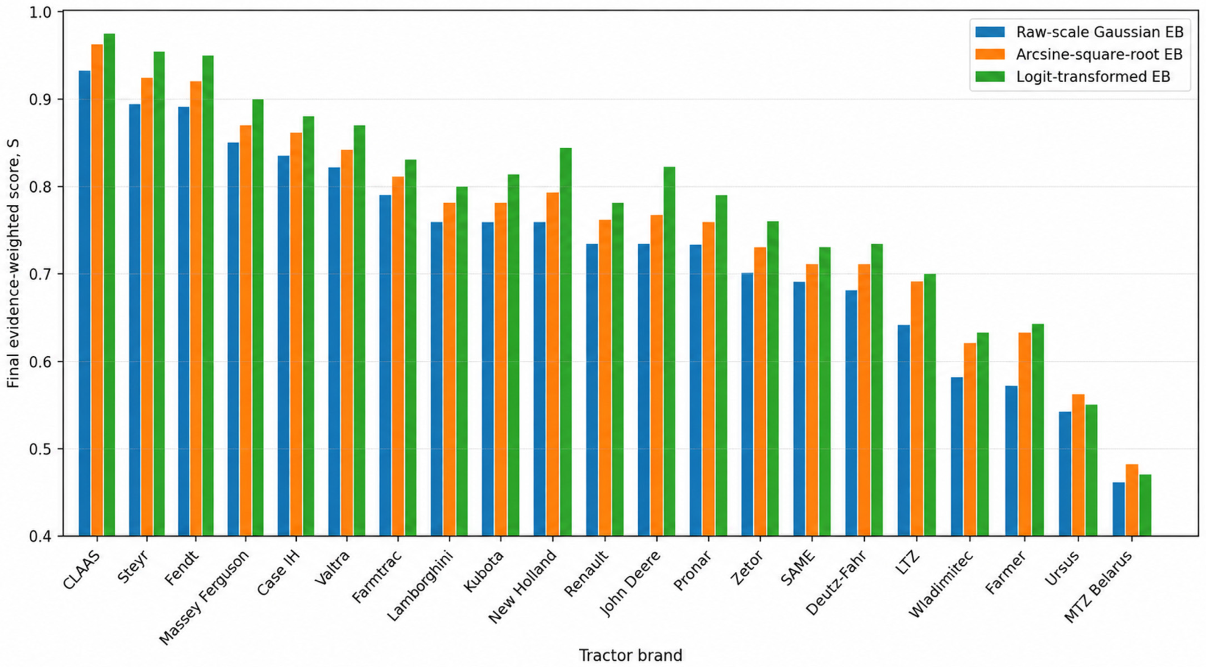
Third, sensitivity to the Gaussian working assumption was evaluated by refitting the hierarchical empirical Bayes model after arcsine-square-root and logit transformations of the normalized scores. For the logit transformation, values were clipped to $\left[\epsilon , 1-\epsilon \right]$, with $\epsilon =0.5/N$ and $N=140$ before transformation. Empirical Bayes estimates were returned to [0, 1] by inverse transformation, and final rankings were compared with the raw-scale Gaussian baseline.

3. Results

3.1. Hierarchical Variance Structure and Evidence Strength

The REML estimates of the domain-specific population means and variance components required for the empirical Bayes regularization are summarized in

Table 2. REML estimates used in the empirical Bayes models.

vg	${\hat{\mathit{\sigma }}}_{\mathit{g}}^{\mathbf{2}}$	${\hat{\mathit{\tau }}}_{\mathit{g}}^{\mathbf{2}}$	${\hat{\mathit{\mu }}}_{\mathit{g}}$	Domain
0.8916	0.02330	0.02613	0.6529	Cabin ($C$)
0.8294	0.02194	0.02645	0.7494	Handling and Usability ($H$)
0.8495	0.02230	0.02625	0.7240	Operation ($O$)
1.1961	0.02786	0.02329	0.7513	Reliability ($R$)
1.1243	0.02580	0.02295	0.7060	External Attributes ($E$)

.

All domains showed positive between-alternative and within-alternative variance components. Equation (8) therefore produced a smooth increase in evidence weight with sample size. In the reliability domain, for example, EEW was approximately 0.46 for $n=1$, 0.72 for $n=3$, 0.91 for $n=12$, and 0.98 for $n=50$.

3.2. Resolution of the Single-Opinion Problem

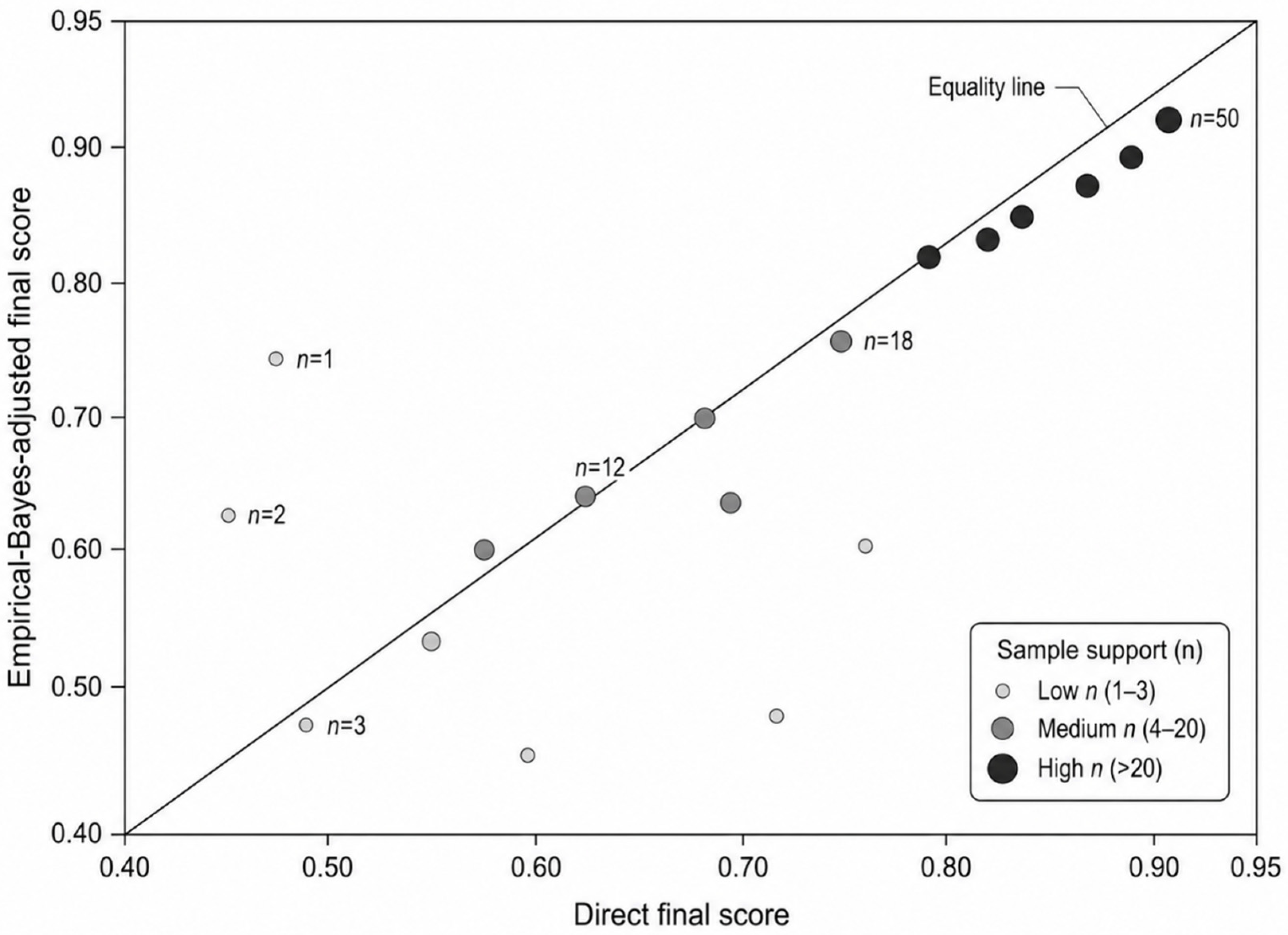
Equation (9) substantially moderated extreme values supported by minimal evidence while leaving data-rich estimates almost unchanged. For Valtra, represented by one respondent, the direct final score decreased from approximately 0.90 to 0.82. Conversely, the one-response Farmer estimate increased from approximately 0.41 to 0.58. The mechanism was symmetric: unsupported favorable and unfavorable extremes were both pulled toward the population structure.

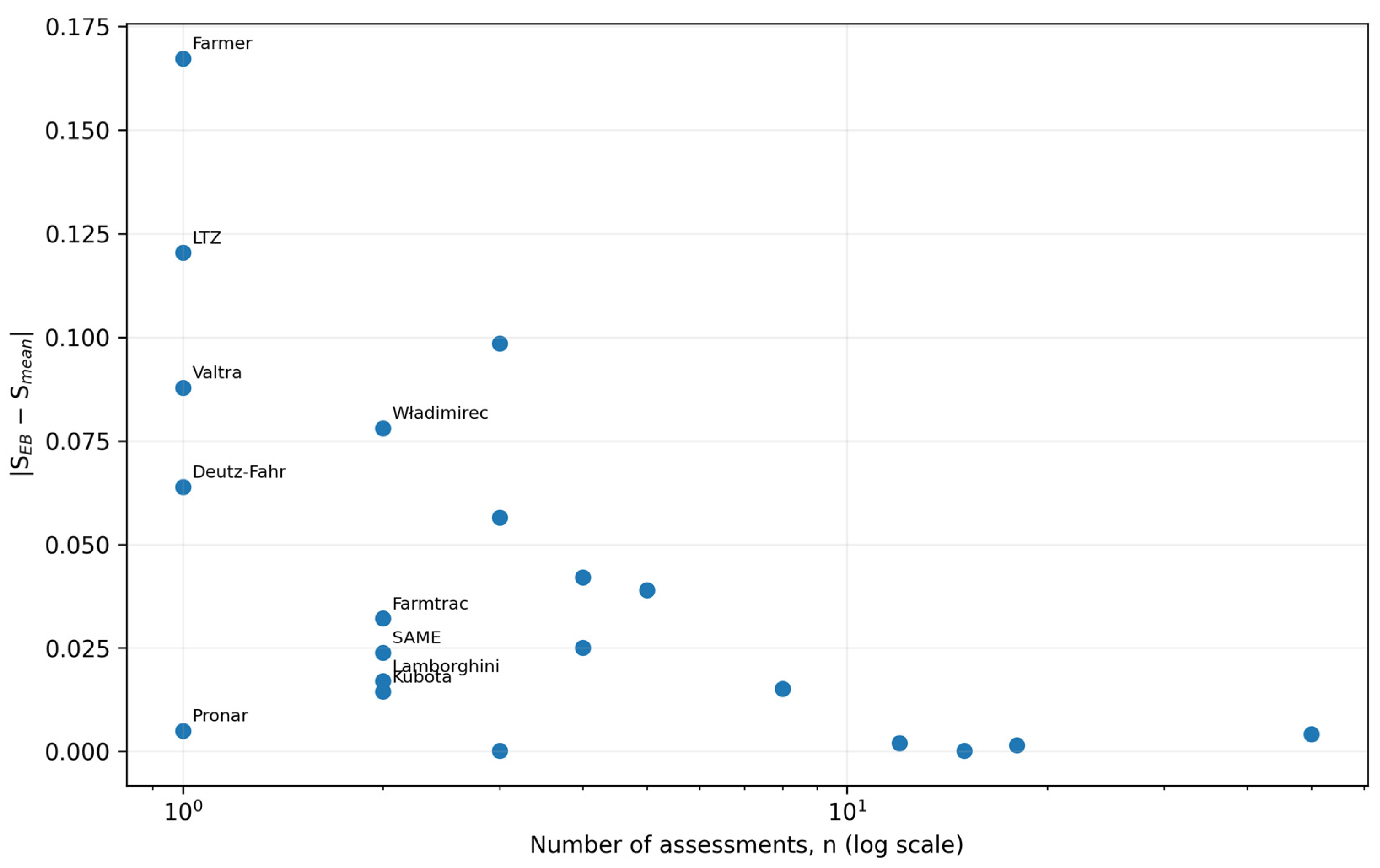
The absolute empirical Bayes correction decreased significantly with sample size (Spearman $\rho =-0.602$, $p=0.0039$. Figure 2 shows the corresponding relationship between direct and adjusted final scores.

3.3. Preservation of Ranking Information

The empirical Bayes adjustment preserved the global structure of the direct ranking. Spearman rank correlation between the direct and adjusted ordering was $\rho =0.992$, while Kendall concordance was $\tau =0.952$. Partial pooling therefore modified weakly supported local extremes without reconstructing the overall ordering. A dedicated benchmark against arithmetic mean, median, fixed-threshold exclusion, and fixed shrinkage is reported in Section 3.7.

3.4. Final Evidence-Weighted Results

The application of the complete evidence-weighted procedure to the AGRORANKING dataset produced the alternative-specific values of inherent quality $Q$, non-inherent attributes $E$, and the final utility index $S$, as summarized in

Table 3. Evidence-weighted AGRORANKING results used as the empirical demonstration.

DAS-7	$\mathit{S}$	$\mathit{E}$	$\mathit{Q}$	$\mathit{n}$	Alternative	Rank
exceptionally high	0.931	0.922	0.934	50	CLAAS	1
very high	0.895	0.890	0.897	3	Steyr	2
very high	0.891	0.854	0.904	4	Fendt	3
very high	0.847	0.859	0.843	8	Massey Ferguson	4
very high	0.830	0.692	0.882	4	Case IH	5
very high	0.815	0.746	0.840	1	Valtra	6
very high	0.789	0.841	0.772	2	Farmtrac	7
very high	0.764	0.694	0.789	2	Lamborghini	8
very high	0.757	0.761	0.756	2	Kubota	9
very high	0.756	0.754	0.756	18	New Holland	10
high	0.733	0.637	0.768	3	Renault	11
high	0.730	0.693	0.742	15	John Deere	12
high	0.727	0.688	0.741	1	Pronar	13
high	0.702	0.740	0.689	12	Zetor	14
high	0.687	0.761	0.664	2	SAME	15
high	0.674	0.648	0.683	1	Deutz-Fahr	16
high	0.641	0.511	0.691	1	LTZ	17
moderate	0.583	0.561	0.591	2	Władimirec	18
moderate	0.576	0.550	0.585	1	Farmer	19
moderate	0.543	0.511	0.554	5	Ursus	20
moderate	0.456	0.516	0.438	3	MTZ Belarus	21

.

The scientific result is not the commercial ordering itself. The important result is that alternatives represented by one and fifty response records coexist within one evidence-weighted model without being treated as equally supported.

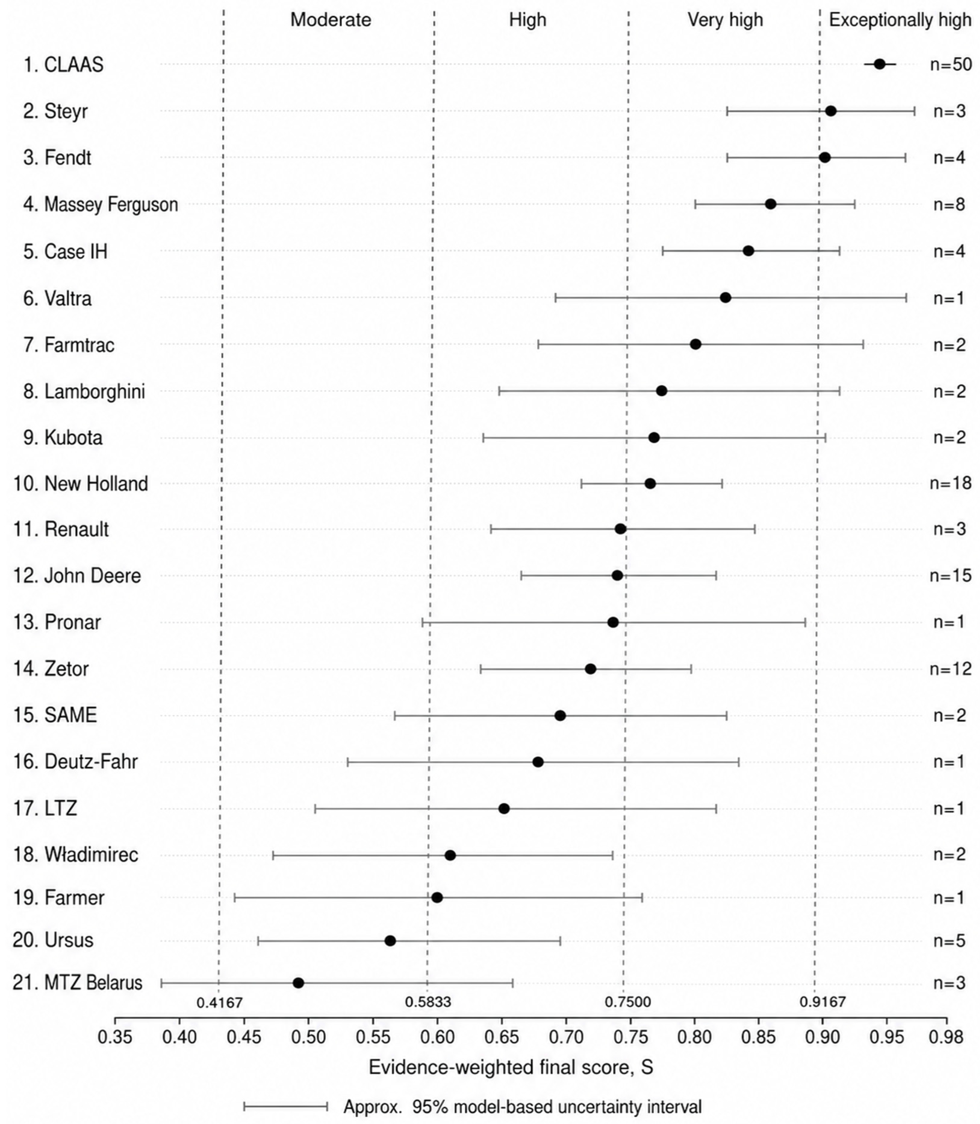
To facilitate interpretation of both the evidence-weighted scores and their uncertainty, Figure 3 presents the final $S$ values for all 21 alternatives together with approximate 95% model-based uncertainty intervals, sample sizes, and the relevant DAS-7 interpretation boundaries.

3.5. Inherent Quality and Non-Inherent Decision Attributes

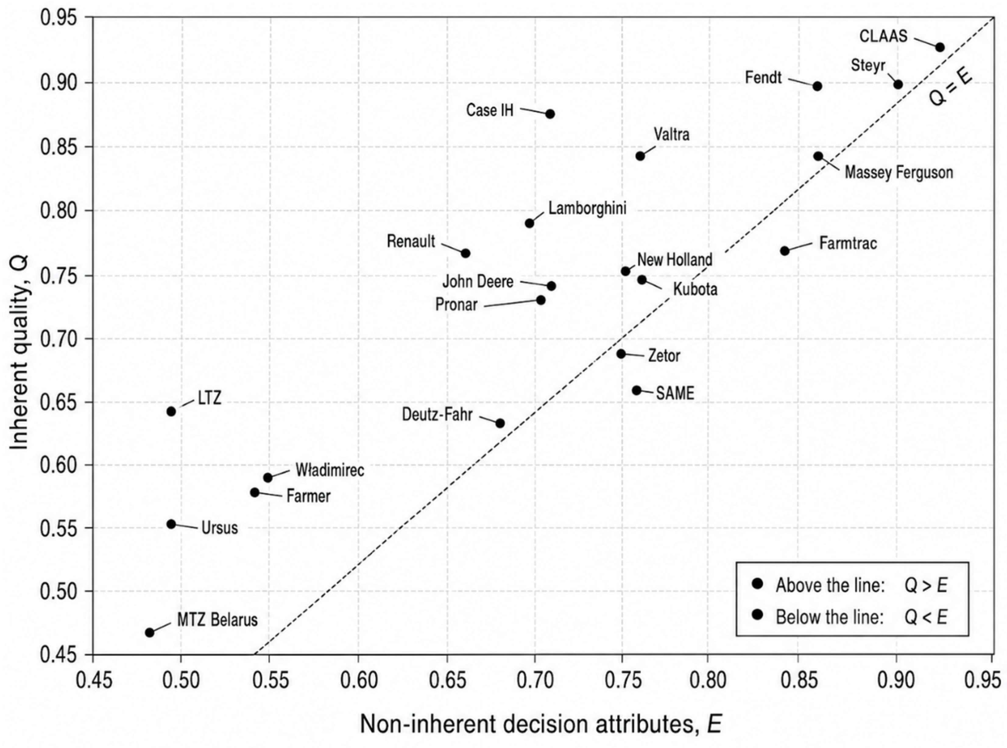
The separation of $Q$ and $E$ revealed distinct decision profiles. For example, Case IH exhibited stronger inherent quality than non-inherent ownership conditions, whereas Farmtrac exhibited the opposite tendency. These profiles would be obscured if all criteria were aggregated at the lowest level.

To examine whether the alternatives exhibit balanced or divergent profiles of inherent quality and non-inherent decision attributes, the empirical Bayes-adjusted $Q$ and $E$ values are compared in Figure 4.

3.6. Probabilistic Ranking

Monte Carlo propagation showed that nominal rank and certainty of rank are distinct. The probability of first position was approximately 0.73 for CLAAS, 0.15 for Steyr, and 0.10 for Fendt. Thus, the deterministic ordering should not be interpreted as a set of certain pairwise superiority statements.

3.7. Empirical Comparison with Simpler Aggregation Strategies

The empirical benchmark showed that evidence weighting preserved the broad ordering contained in the raw assessments while moderating unsupported small-sample extremes. Relative to empirical Bayes, arithmetic mean aggregation produced Spearman $\rho =0.992$ and Kendall $\tau =0.952$, with a mean absolute rank shift of 0.48 positions and a maximum shift of two positions. Median aggregation yielded $\rho =0.982$ and $\tau =0.924$, with a mean absolute rank shift of 0.76 and a maximum shift of three positions.

The principal difference concerned score dispersion. The standard deviation of final $S$ scores was 0.122 for empirical Bayes, compared with 0.175 for the arithmetic mean and 0.181 for the median. For the $n=1$ alternatives, Valtra decreased from a direct score of approximately 0.903 to an empirical Bayes score of 0.815, whereas Farmer increased from approximately 0.409 to 0.576. The procedure therefore moderated both favorable and unfavorable unsupported extremes rather than systematically penalizing small samples.

A hard threshold of $n\ge 3$ retained only 11 of 21 alternatives and excluded 10, corresponding to 47.6% of the brands. The fixed-target shrinkage estimator retained all alternatives but compressed final score dispersion to 0.088.

Table 4. Empirical comparison of the proposed evidence-weighted estimator with simpler aggregation strategies.

SD of $\mathit{S}$	Max Rank Shift	Mean abs. Rank Shift	Kendall $\mathit{\tau }$ vs. EB	Spearman $\mathit{\rho }$ vs. EB	Retained/ Excluded	Method
0.122	0	0.00	1.000	1.000	21/0	Empirical Bayes
0.175	2	0.48	0.952	0.992	21/0	Arithmetic mean
0.181	3	0.76	0.924	0.982	21/0	Median
0.187 *	1 *	0.18 *	0.964 *	0.991 *	11/10	Fixed threshold $n$ ≥ 3
0.088	2	0.48	0.952	0.992	21/0	Fixed shrinkage

* Calculated only for the 11 alternatives retained under the threshold rule.

summarizes the comparison.

Figure 5 visualizes the evidence-dependent moderation of the direct scores and shows that the largest corrections occur for the sparsely represented alternatives.

3.8. Simulation-Based Validation

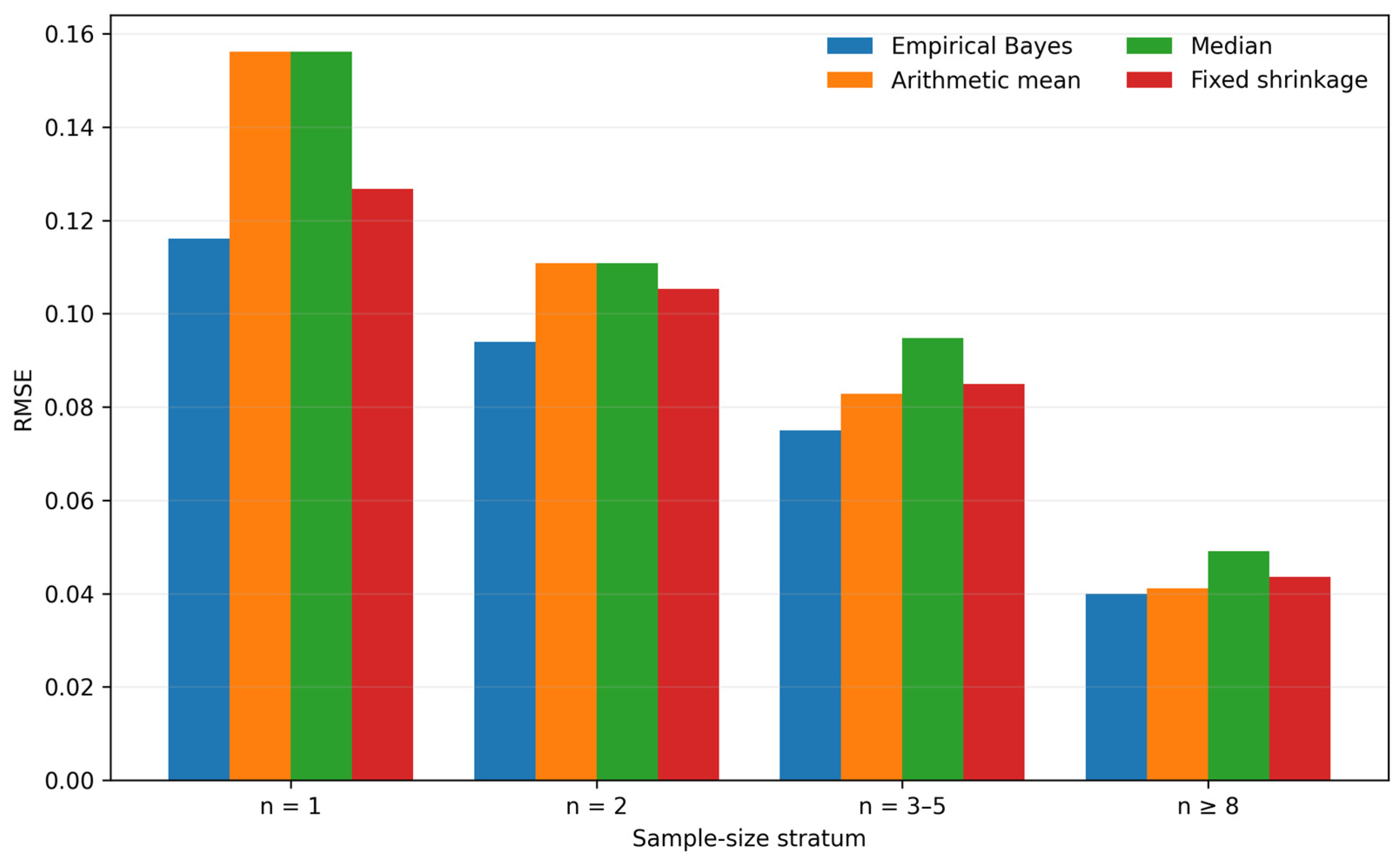
Under the correctly specified Gaussian hierarchy, empirical Bayes achieved the lowest overall $\mathrm{R}\mathrm{M}\mathrm{S}\mathrm{E}$ (0.0854), compared with 0.1053 for the arithmetic mean, 0.1090 for the median, and 0.0948 for fixed shrinkage. Bias was close to zero for all methods. The advantage was strongest at $n=1$, where empirical Bayes $\mathrm{R}\mathrm{M}\mathrm{S}\mathrm{E}$ was 0.1161 versus 0.1562 for both direct mean and median, corresponding to an approximately 26% reduction relative to direct averaging. At $n\ge 8$, empirical Bayes and arithmetic mean $\mathrm{R}\mathrm{M}\mathrm{S}\mathrm{E}$ values converged to 0.0399 and 0.0411, respectively.

The bounded non-Gaussian stress test produced the same qualitative result. Empirical Bayes $\mathrm{R}\mathrm{M}\mathrm{S}\mathrm{E}$ was 0.0818, compared with 0.0983 for the arithmetic mean, 0.1033 for the median, and 0.0932 for fixed shrinkage. Ranking recovery was also competitive: empirical Bayes produced the highest top-one recovery probability in both scenarios (0.476 and 0.494). Fixed shrinkage yielded marginally higher mean Spearman rank correlation but substantially poorer interval coverage (0.704 and 0.680), indicating overconfident uncertainty representation.

These results show that partial pooling improves estimation primarily where evidence is sparse and that the benefit persists under bounded non-Gaussian data generation.

Table 5. Performance of alternative estimators in the controlled simulation study.

Mean abs. Rank Error	Top-One Recovery	Spearman $\mathit{\rho }$	95% Coverage	$\mathbf{R}\mathbf{M}\mathbf{S}\mathbf{E}$	Bias	Scenario/Method
2.82	0.476	0.795	0.930	0.0854	0.0002	Gaussian/Empirical Bayes
2.85	0.441	0.786	0.948	0.1053	0.0001	Gaussian/Arithmetic mean
2.95	0.435	0.774	0.973	0.1090	0.0001	Gaussian/Median
2.86	0.428	0.799	0.704	0.0948	0.0002	Gaussian/Fixed shrinkage
2.70	0.494	0.811	0.927	0.0818	−0.0004	Bounded/Empirical Bayes
2.72	0.438	0.804	0.940	0.0983	0.0001	Bounded/Arithmetic mean
2.80	0.469	0.796	0.954	0.1033	0.0071	Bounded/Median
2.75	0.406	0.815	0.680	0.0932	−0.0001	Bounded/Fixed shrinkage

summarizes the complete simulation results.

Figure 6 isolates the sample-size dependence of estimation error under Scenario A.

3.9. Robustness to Preference and Distributional Assumptions

The final ranking was highly stable to the upper-level quality weight parameter $\alpha$. Across $\alpha =0.50÷0.90$, Spearman correlation with the baseline $\alpha =0.75$ ranking ranged from 0.977 to 1.000. Within $\alpha =0.70÷0.90$, $\rho$ remained between 0.995 and 1.000, and the maximum rank shift was at most one position. The top-ranked alternative remained unchanged across the complete range, and the top-five composition was fully preserved for $\alpha \ge 0.65$.

AHP preference weight perturbations produced even smaller changes. Across 10,000 stochastic perturbations, mean Spearman correlation with the baseline ranking was 0.9992, and the fifth percentile was 0.9961. The mean maximum rank displacement was 0.46 positions, the 95th percentile was two positions, and the baseline top-ranked alternative remained first in all perturbations. One-at-a-time ±20% changes to individual AHP weights produced at most a one-position shift.

Distributional sensitivity was similarly limited. Relative to the raw-scale Gaussian model, the arcsine-square-root model produced Spearman $\rho =0.992$ and a maximum rank shift of two positions, while the logit-transformed model produced $\rho =0.975$ and a maximum shift of three positions. The identity of the top-ranked alternative and the complete top-five composition were unchanged under both transformed models.

Table 6. Sensitivity of the final ranking to $\alpha$, AHP weights, and bounded score distributional treatment.

Top-5 Preserved	Top-Ranked Alternative	Max Rank Shift	Spearman $\mathit{\rho }$ vs. Baseline	Condition	Sensitivity Analysis
4/5	CLAAS	4	0.977	0.50	$\alpha$
5/5	CLAAS	1	0.999	0.70	$\alpha$
5/5	CLAAS	0	1.000	0.80	$\alpha$
5/5	CLAAS	1	0.995	0.90	$\alpha$
Highly stable	CLAAS	95th percentile = 2	mean 0.999	10,000 perturbations	AHP weights
5/5	CLAAS	2	0.992	Arcsine-square-root EB	Distribution
5/5	CLAAS	3	0.975	Logit-transformed EB	Distribution

and Figure 7 summarize these results.

The grouped comparison in Figure 7 shows the final scores under the three distributional treatments.

4. Discussion

4.1. From Product Ranking to OR/MCDM Decision Support

The principal contribution extends beyond ranking. The framework separates measurement, evidence strength, preference weighting, quality synthesis, uncertainty, and decision support. Many deterministic MCDM procedures treat alternative performance scores as fixed inputs; here, the scores themselves are uncertain and unequally supported. This separation aligns the method with contemporary uncertainty-aware MCDM and engineering decision support research [3,4,5,6].

4.2. Why Directly Measurable Attributes Are Outside the Core Method

A directly measurable attribute has an objective reference scale and can be compared after standardization. The present framework addresses the harder class of attributes whose practically relevant assessment must be elicited through structured user judgment. This does not imply that physical measurements are unimportant; they can be integrated into a broader decision model, but they do not require the evidence regularization mechanism developed here.

4.3. Why the Arithmetic Mean Alone Is Insufficient

The direct mean is transparent and maximally discriminating, but it assigns the same point-estimate status to $n$ = 1 and $n$ = 50. The empirical benchmark now quantifies this distinction: the arithmetic mean and empirical Bayes rankings were strongly correlated ($\rho$ = 0.992), yet direct scores were substantially more dispersed (SD = 0.175 versus 0.122). The empirical Bayes correction therefore preserves the broad ordering while stabilizing unsupported extremes rather than adding sample size directly to the final quality score.

4.4. Why a Fixed Minimum Sample Size Was Rejected

A fixed threshold is operationally simple but creates an arbitrary discontinuity between inclusion and exclusion. In the present data, even the relatively permissive rule $n\ge 3$ retained only 11 of 21 alternatives and removed 47.6% of the brands. The continuous EEW avoids this information loss by representing evidence strength continuously rather than converting it into a binary eligibility decision.

4.5. Why Median and Mode Were Not Selected

Median aggregation is robust to isolated extremes but does not represent evidence strength and can reduce numerical resolution on a discrete rating scale. In the present benchmark, its ranking remained broadly similar to empirical Bayes ($\rho$ = 0.982) but produced larger mean and maximum rank shifts and greater final score dispersion. No exact ties occurred in the final composite $S$ for this dataset, so the empirical argument is not that median aggregation necessarily creates ties, but that it is less adaptive to sample-size imbalance than variance-based partial pooling [13,14].

4.6. Why the Harrington Desirability Function Was Rejected

A Harrington-type desirability transformation was considered because it offers an elegant nonlinear mapping of a response into a dimensionless desirability measure [17,18]. In its classical one-sided form,

$$d\left(y\right)=\mathrm{e}\mathrm{x}\mathrm{p} \left[-\mathrm{e}\mathrm{x}\mathrm{p}\left(-y\right)\right]$$

(17)

The function satisfies $\underset{y\to -\infty }{\lim }d\left(y\right)=0$ and $\underset{y\to \infty }{\lim } d\left(y\right)=1$. However, for every finite $y$,

$$0<d\left(y\right)<1,\hspace{1em}y\in \mathbb{R}.$$

(18)

This property is crucial for the present measurement problem. The source seven-category scale has finite, substantively defined end points. Rating 1 is the minimum admissible state and rating 7 is the maximum admissible state. Under the affine transformation in Equation (4), these are mapped exactly to zero and one. The classical Harrington function can reach exact desirability values of zero and one only asymptotically, so it cannot preserve both finite end points without additional arbitrary rescaling or truncation.

A second objection concerns the center of the scale. In the nonlinear variant examined during methodological development, the neutral source response 4/7 mapped to approximately 0.37 desirability. The transformation would therefore impose the substantive claim that a neutral state is already distinctly unfavorable. No independent engineering or behavioral calibration supported that assumption. The nonlinear function would also make identical one-category changes have different numerical consequences depending on their location on the scale.

For these reasons, the affine normalization was retained. It maps 1 to 0, 4 to 0.5, and 7 to 1 exactly. Statistical sophistication is introduced at the evidence inference stage, where regularization is supported by the observed variance structure, rather than through an unvalidated nonlinear utility transformation of the measurement scale.

4.7. Why the Earlier Ten-Class Classification Was Rejected

A ten-class external quality scale does not arise naturally from a seven-category source instrument. DAS-7 follows directly from seven source anchors and six midpoint boundaries. Its advantage is not that seven classes are universally superior, but that measurement and interpretation remain structurally congruent.

4.8. Why Bootstrap Does Not Solve the Single-Opinion Problem

Bootstrap procedures are useful for uncertainty assessment but cannot create independent information. At $n=1$, every conventional bootstrap resample contains the same observation. Hierarchical partial pooling addresses a different problem by borrowing strength from the population of related alternatives. Bootstrap can therefore be supplementary, but it is not a solution to missing evidence.

4.9. Why an Arbitrary Technical Tie Threshold Was Rejected

A fixed rule such as $\left|S_j-S_j^{\prime }\right|<0.02$ is simple but has no universal inferential meaning. The evidential meaning of the same numerical difference depends on sample size and variance. Probability of superiority and rank probabilities therefore provide a more defensible representation than an arbitrary universal tie margin.

4.10. Why Empirical Bayes with REML Was Selected

The selected architecture retains the resolution of arithmetic means while reducing sparse sample instability. This claim is now supported by controlled simulation with known truth. Under the correctly specified hierarchy, empirical Bayes reduced overall $\mathrm{R}\mathrm{M}\mathrm{S}\mathrm{E}$ from 0.1053 for the arithmetic mean to 0.0854, and at $n=1$ from 0.1562 to 0.1161. The advantage persisted under bounded non-Gaussian generation ($\mathrm{R}\mathrm{M}\mathrm{S}\mathrm{E}$ 0.0818 versus 0.0983). Thus, the $n=1$ estimate is not assumed to be intrinsically better because it is closer to the population mean; rather, partial pooling reduced expected estimation error under the simulated hierarchical structures. REML estimates the variance structure from the data and empirical Bayes converts that structure into continuous partial pooling [7,8,9,10,11,12].

4.11. Why B Is an Evidence Weight Rather than Credibility

A value such as $B_{jg}=0.50$ does not mean that an assessment is 50% reliable or has a 50% probability of being true. It describes the balance between alternative-specific and population-level information under the fitted hierarchical model. The term Empirical Evidence Weight is therefore used deliberately.

4.12. Why AHP Preference Weight and Evidence Weight Must Remain Separate

The AHP coefficient $w_r$ represents the preference importance of domain $r$. The empirical Bayes coefficient $B_{jg}$ represents the evidence supporting alternative $j$ in domain $g$. Combining these concepts would mix preference with inference. The explicit separation between them is a central methodological feature of the proposed MCDM architecture.

4.13. Why Inherent and Non-Inherent Attributes Are Separated

The division between $Q$ and $E$ follows the adopted quality concept [13]. A technical deficiency implies a design or engineering issue; an unfavorable service or parts environment implies an organizational or market issue. Keeping these dimensions separate until final synthesis increases diagnostic interpretability.

4.14. Why the Final Aggregation Is Geometric

A simple additive utility is fully compensatory. A serious deficiency in inherent quality could therefore be offset by favorable ownership conditions. The weighted geometric function reduces this possibility while preserving monotonicity, which is appropriate when both upper-level dimensions should remain substantively relevant. It does not, however, provide complete non-compensation or a criterion-specific veto mechanism. ELECTRE-type outranking or explicit veto thresholds would therefore represent a meaningful extension when unacceptable performance on a single criterion must preclude an otherwise favorable alternative.

4.15. Uncertainty and Decision Risk Are Not Synonyms

Uncertainty concerns incomplete knowledge of the alternatives; decision risk additionally depends on the consequences of acting under that uncertainty. The present rank probabilities quantify decision-relevant uncertainty. Expected opportunity loss can be added when the decision maker wishes to introduce an explicit loss structure, consistent with the OR perspective [3,6].

4.16. General Applicability, Robustness, and Limitations

The method is not specific to tractors and can be transferred to other products whenever subjective attributes are decision-relevant and evidence is sparse or unequal. The sensitivity results reduce, but do not eliminate, several modeling concerns: rankings were stable across $\alpha =0.50÷0.90$, under 10,000 AHP weight perturbations, and after arcsine-square-root and logit transformations of the bounded scores. Nevertheless, the Gaussian model remains a working approximation; REML hyperparameters are treated conditionally, domains are modeled independently, and AHP preferences remain application-specific. The semantic interpretation of DAS-7 is measurement-derived rather than externally validated and should be validated against independent behavioral or engineering criteria in future studies. The tractor results must also be interpreted as aggregated user-reported experiential quality rather than isolated causal brand effects. Tractor age, operating intensity, maintenance history, model composition, and other usage conditions were not jointly controlled. The anonymous dataset permits verification of 140 unique response records but not independent identity verification across separate submissions. In addition, the current framework summarizes central tendency and uncertainty but does not explicitly encode alternative-specific response polarization: two alternatives with similar means but different within-alternative response distributions may therefore require an additional dispersion descriptor such as SD or IQR. Empirical Bayes cannot manufacture information; an alternative represented by one record remains uncertain, but its evidential weakness is represented explicitly rather than ignored. In particular, the observed positive cross-domain correlations mean that independent domain-wise uncertainty propagation may understate aggregate uncertainty; this should be addressed in future work using a multivariate hierarchical formulation.

The main methodological alternatives considered during development of the framework, together with their advantages, limitations, and final status, are summarized in

Table 7. Methodological alternatives considered during framework development.

Status	Critical Limitation	Advantage	Approach
Intermediate only	Small-$n$ instability	High resolution	Arithmetic mean
Rejected	Information loss and discontinuity	Simple safeguard	Fixed $n$ threshold
Rejected	Loss of discrimination	Robust	Median/mode
Rejected	Finite endpoints not mapped exactly to 0/1; unvalidated utility	Smooth nonlinear mapping	Harrington desirability
Supplementary	Creates no new information at tiny $n$	Useful uncertainty tool	Bootstrap
Rejected	Arbitrary and uncertainty blind	Simple	Fixed ΔS tie
Selected	Model dependent	Data-driven variance estimation	REML
Selected	Hierarchical assumptions	Continuous evidence weighting	Empirical Bayes
Selected	Decision maker dependent	Explicit preference weighting	AHP
Selected	External validation still needed	Measurement congruence	DAS-7

.

5. Conclusions

This study developed and quantitatively validated an evidence-weighted OR/MCDM framework for subjective product quality assessment under sparse and strongly unbalanced information. Its principal methodological contribution is the explicit separation of respondent-level measurement, evidence strength, preference weighting, inherent quality, non-inherent decision attributes, and uncertainty within one reproducible decision support architecture.

The empirical benchmark showed that partial pooling preserved the broad ranking structure of direct aggregation (Spearman $\rho =0.992$) while moderating unsupported extremes and avoiding the information loss created by hard sample-size thresholds. A controlled simulation with known truth provided stronger validation: empirical Bayes achieved the lowest $\mathrm{R}\mathrm{M}\mathrm{S}\mathrm{E}$ under both the correctly specified Gaussian hierarchy and the bounded non-Gaussian stress test, with the greatest improvement for $n=1$ and progressively smaller differences as evidence increased.

The main conclusions were also robust to decision and distributional assumptions. Ranking stability remained high across $\alpha =0.50÷0.90$, across 10,000 perturbations of AHP weights, and under arcsine-square-root and logit treatments of bounded scores. These analyses support the interpretation of the method as an adaptive evidence regularizer rather than a ranking replacement.

The framework supports multi-criteria decision making for complex products when important quality attributes cannot be compared directly using objective physical measurements and must instead be inferred from structured user experience. Agricultural tractors provide the present real-world demonstration, but the architecture is transferable to other decision problems with sparse subjective evidence. Its limitations remain important: the application does not identify causal brand effects, alternative-specific response polarization is not modeled explicitly, the geometric utility does not implement a veto mechanism, and DAS-7 requires external semantic validation. Weak evidence should therefore neither be discarded nor treated as strong evidence; its influence and uncertainty should be quantified explicitly.