An Improved DeepLabV3+ Network for Bare Rock Segmentation in Remote Sensing Images

Abstract

To improve the binary semantic segmentation of bare rock and background in complex urban environments, this study developed an improved DeepLabV3+ model for red–green–blue (RGB) imagery derived from Gaofen-1 (GF-1) data. Four backbone networks—Xception, ResNet50, MobileNetV2, and MobileNetV3—were first evaluated. ResNet50 was selected because it achieved the highest bare-rock IoU and bare-rock F1-score among the evaluated backbones under the evaluated experimental configuration. An Adam-based training configuration was subsequently evaluated against a stochastic gradient descent (SGD)-based configuration and selected for the ResNet50 baseline. Squeeze-and-excitation (SE) channel attention, a spatial attention module (SATM), and a receptive field block (RFB) were then integrated to enhance feature representations from channel, spatial, and multi-scale perspectives. In the repeated evaluation of the proposed model within the ablation experiment using three independent training runs, the model achieved a mean bare-rock IoU of 79.36 ± 0.30%, a mean bare-rock precision of 88.65 ± 0.55%, and a mean bare-rock F1-score of 88.49 ± 0.19%. These results indicate favorable overall bare-rock segmentation performance under the evaluated experimental setting. Compared with the original DeepLabV3+ configuration (Xception + SGD), the proposed model achieved improvements of 14.51, 4.80, and 9.82 percentage points in bare-rock IoU, precision, and F1-score, respectively. These improvements reflect the combined effects of backbone selection, optimizer configuration, and the proposed module integration. Compared with the ResNet50 + Adam baseline model established in this study, the proposed model further improved these metrics by 5.19, 4.60, and 3.32 percentage points, respectively. Among the evaluated models, the proposed method achieved the highest bare-rock IoU and bare-rock F1-score, whereas U-Net achieved a higher bare-rock precision. Thus, the comparative advantage of the proposed model was primarily reflected in segmentation overlap and overall F1 performance rather than in precision. Qualitative comparisons further showed favorable boundary continuity and feature discrimination in representative complex urban scenes containing buildings, vegetation, roads, and shadow-affected areas. These results provide methodological support for bare-rock segmentation and related geological remote-sensing applications in complex plateau urban environments.

1. Introduction

From a strict geological and remote sensing perspective, bare rock is defined as bedrock or consolidated mineral aggregates that are exposed on the surface and have little vegetation, soil, or artificial cover. Xining, situated in the eastern Qinghai–Xizang Plateau, is a major transportation hub and an important component of the regional ecological barrier. Its core urban districts—Chengdong, Chengzhong, and Chengxi—lie in the transitional zone between the Huangshui Valley and the loess hills. The region contains extensive bare-rock exposures, and accurate delineation of bare rock from surrounding background classes, including buildings, vegetation, and water bodies, is relevant to geological-hazard assessment, ecological-restoration planning, infrastructure development, and mineral exploration [1,2,3,4,5].

Remote sensing technology provides an efficient means of acquiring and analyzing large-area geological and land-surface information [6]. Multispectral remote sensing data, characterized by their extensive spectral band coverage, effectively capture the differences among various ground objects across multiple spectral channels [7,8]. With the continued development of remote-sensing technology, multi-source remote-sensing data have been widely used in geological-structure interpretation, mineral-resource exploration, and geological-hazard monitoring, enabling efficient acquisition and analysis of geological information [9,10,11]. In recent years, deep-learning-based semantic segmentation has advanced from early fully convolutional networks (FCNs) and U-Net to Transformer-based architectures such as SegFormer and, more recently, visual foundation models and general-purpose segmentation models. These developments have expanded the capacity of segmentation models to represent complex spatial and contextual information in remote-sensing imagery. Recent studies have explored approaches for addressing label scarcity, cross-domain generalization, and scale variation by integrating hyperbolic-space representations, visual foundation models, and task-specific prior knowledge [12,13]. Among commonly used semantic segmentation architectures, DeepLabV3+ has been widely applied to remote-sensing image segmentation because its encoder–decoder structure and Atrous Spatial Pyramid Pooling (ASPP) module support multi-scale contextual representation [14,15,16]. DeepLabV3+ has been adapted for different application scenarios. For lightweight deployment, depthwise separable convolutions and MobileNet-series backbones have been introduced to reduce model parameters and computational cost while maintaining competitive segmentation performance [17,18,19]. Deep-learning methods have also been applied to the recognition and segmentation of geological and land-surface targets, including lithological classification, coal–rock recognition, and bare-soil extraction, demonstrating their ability to learn discriminative visual and contextual features from complex images [20,21,22]. For detailed rock-mass characterization, CNN-based methods have been applied to detect discontinuities in 3D point clouds, while multi-scale attention models have been used to identify rock fractures [23,24]. In specific complex-scene extraction tasks, improved DeepLabV3+ models have been applied to bare-rock extraction from high-resolution UAV imagery and forest-road extraction from satellite imagery [25,26]. In high-altitude cold-region environments, dual-encoder networks combined with multispectral imagery have also been applied to the automatic identification of rock and glacier-related targets [27]. Recent attention-enhanced DeepLabV3+ studies have introduced multi-scale attention for tailings-pond identification, adaptive multi-statistic fusion attention for GF-1 sea-ice segmentation, ECA attention for landslide recognition, and CBAM for crop extraction. These studies demonstrate the effectiveness of attention-enhanced DeepLabV3+ in different application scenarios. In contrast, the present study focuses on bare-rock segmentation from GF-1 RGB imagery in complex plateau urban environments and develops a task-oriented integration strategy by combining a comparatively selected ResNet50 + Adam baseline with SE channel attention, a spatial attention module (SATM), and RFB receptive-field enhancement. The methodological innovation accordingly lies in the coordinated adaptation and evaluation of these complementary mechanisms for the specific problems of feature confusion, boundary ambiguity, and target-scale variation in plateau urban bare-rock segmentation. Some existing lithology interpretation approaches rely on multi-source heterogeneous remote-sensing data, which can increase data requirements and may limit their direct applicability to binary bare-rock segmentation using single-sensor GF-1 imagery after standard image fusion processing.

In summary, existing geological remote-sensing studies have largely focused on broader-scale applications, while fine-scale bare-rock segmentation in complex plateau urban environments remains comparatively underexplored. Existing DeepLabV3+-based methods do not always address visual-feature confusion, boundary ambiguity, and target-scale variation simultaneously in plateau urban RGB imagery. Given the high implementation cost of large-scale models and the limited comparative verification available for this task, this study uses GF-1 imagery of the main urban area of Xining to develop and evaluate an improved DeepLabV3+ network based on a ResNet50 + Adam baseline with SE, SATM, and RFB modules. The resulting model was evaluated through ablation experiments, internal model comparisons, and external validation for the binary semantic segmentation of bare rock and background in complex plateau urban environments. Specifically, different backbone networks and optimizers were first compared to establish the ResNet50 + Adam baseline for subsequent module integration. On this basis, SE channel attention, SATM-based spatial attention, and RFB receptive-field enhancement modules were further integrated to alleviate feature confusion, blurred boundaries, and difficulties in recognizing bare-rock targets at different scales. The main contributions of this article are as follows:

• A task-oriented DeepLabV3+ improvement strategy is developed for GF-1 bare-rock segmentation in complex plateau urban environments. Based on comparative selection of the ResNet50 backbone and Adam optimizer, SE channel attention, SATM-based spatial attention, and RFB receptive-field enhancement are coordinately integrated to strengthen channel, spatial, and multi-scale feature representation, thereby forming a targeted methodological framework for addressing feature confusion, boundary ambiguity, and scale variation of bare-rock targets.
• The proposed architecture combines channel, spatial, and multi-scale feature modeling to improve feature discrimination and boundary representation in urban scenes containing buildings, vegetation, and shadow-affected areas.
• The proposed GF-1-based framework provides a methodological basis for bare-rock segmentation in plateau cities and may support applications such as geological-hazard monitoring, ecological-environment assessment, and bare-rock interpretation in similar plateau river-valley environments.

2. Materials and Methods

2.1. Study Area and Data Sources

2.1.1. Study Area

The study area is situated in the core zone of Xining City, Qinghai Province, encompassing the Chengdong, Chengzhong, and Chengxi Districts. This region lies within the middle reaches of the Huangshui Valley, with geographical coordinates ranging from 101°49′ E to 101°59′ E longitude and 36°34′ N to 36°49′ N latitude. The three urban districts are arranged in a zonal pattern along the northern and southern banks of the Huangshui River, covering a total area of approximately 318.57 km². This area serves as a crucial geographical node and regional transportation hub in eastern Qinghai. The region exhibits a plateau continental climate, characterized by an annual average temperature of 5.1 °C and annual precipitation of 371.2 mm. It is marked by high evaporation rates, ample sunshine, and a notable diurnal temperature variation. The city is intersected by three rivers: the Huangshui River, the Nanchuan River, and the Beichuan River. Urban areas are characterized by extensive artificial afforestation, with green coverage exceeding 40%. The terrain is higher in the southwest and gradually decreases toward the northeast, with an average elevation of 2261 m and predominantly valley-plain landforms. Geologically, the region is classified within the Hehuang Valley stratigraphic area of the eastern Qilian Mountains. Quaternary strata, including sandy gravel, silt, and silty clay, are widely distributed, while Tertiary red beds comprising mudstone and sandstone are locally exposed along the margins of the study area, forming typical bare-rock exposures. These characteristics provide representative conditions for evaluating the binary semantic segmentation of bare rock and background in a complex plateau urban environment.

2.1.2. Data Sources

The training, validation, and test data in this study were derived from GF-1 PMS2 Level-1A imagery provided by the Comprehensive Information Service Platform for High-Resolution Applications of Qinghai Province. The source imagery was georeferenced in the WGS 84 geographic coordinate system. Following orthorectification, the imagery was projected to WGS 84/UTM Zone 47N for subsequent spatial processing and distance analysis. The original panchromatic and multispectral spatial resolutions were 2 m and 8 m, respectively. After pan-sharpening, the fused imagery had a spatial resolution of 2 m. The imagery used for model training, validation, and internal testing was acquired at 12:01:20 on 24 September 2024. The image covered approximately 1186.53 km², with 2% cloud cover and no snow. At acquisition, the solar azimuth, solar zenith angle, sensor side-swing angle, and satellite zenith angle were 154.76°, 40.03°, 0°, and 1.68°, respectively. The four corner coordinates were (36.764303° N, 101.594241° E), (36.694157° N, 101.968242° E), (36.391185° N, 101.880217° E), and (36.461183° N, 101.507664° E).

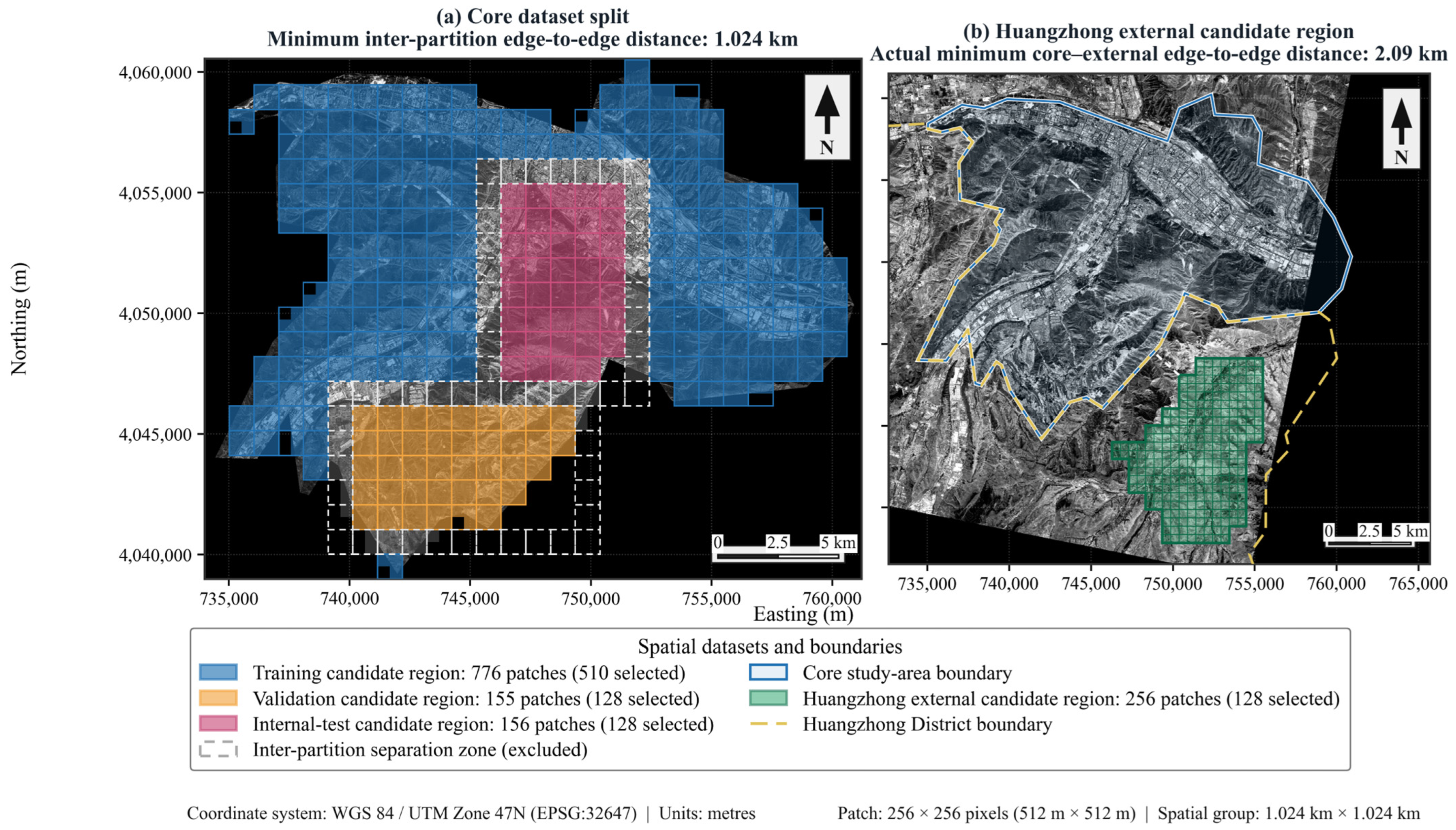
For external evaluation, GF-1 PMS2 Level-1A imagery acquired over the adjacent Huangzhong District at 12:02:06 on 28 May 2025 was used to construct a spatially distinct, external test set. The image covered approximately 426.3 km² in the northern part of Huangzhong District, with no clouds or snow. At acquisition, the solar azimuth, solar zenith angle, sensor side-swing angle, and satellite zenith angle were 130.74°, 21.16°, 0°, and 1.69°, respectively. The four corner coordinates were (36.58° N, 101.52° E), (36.51° N, 101.86° E), (36.32° N, 101.79° E), and (36.39° N, 101.45° E). During external sample selection, a 1.024-km geographic separation buffer was retained along the boundary between the core study area and Huangzhong District. Candidate patches within the potential overlap extent of the two GF-1 scenes or along invalid image edges were also excluded. After spatial exclusion, the retained Huangzhong external candidate region contained 256 candidate patches. The actual minimum edge-to-edge distance between the core study-area boundary and the retained external candidate region was 2.09 km, exceeding the predefined 1.024-km separation requirement. The remaining external candidate patches were jointly screened by the same three researchers according to image validity, bare-rock occurrence, and representative background conditions. The eligible candidate patches were subsequently categorized at the patch level according to whether valid bare-rock pixels were present in the reference labels. A stratified purposive selection strategy was used to include both bare-rock-containing scenes and representative complex background scenes. To avoid constructing an external test set consisting exclusively of bare-rock-containing patches, representative background-only patches containing no valid bare-rock pixels were additionally included. The final external test set consisted of 128 non-overlapping 256 × 256-pixel patches, including 119 bare-rock-containing patches and 9 background-only patches. Background-only patches contained no valid bare-rock pixels and were included to represent background-dominated scenes and assess false-positive predictions.

2.2. Research Methods

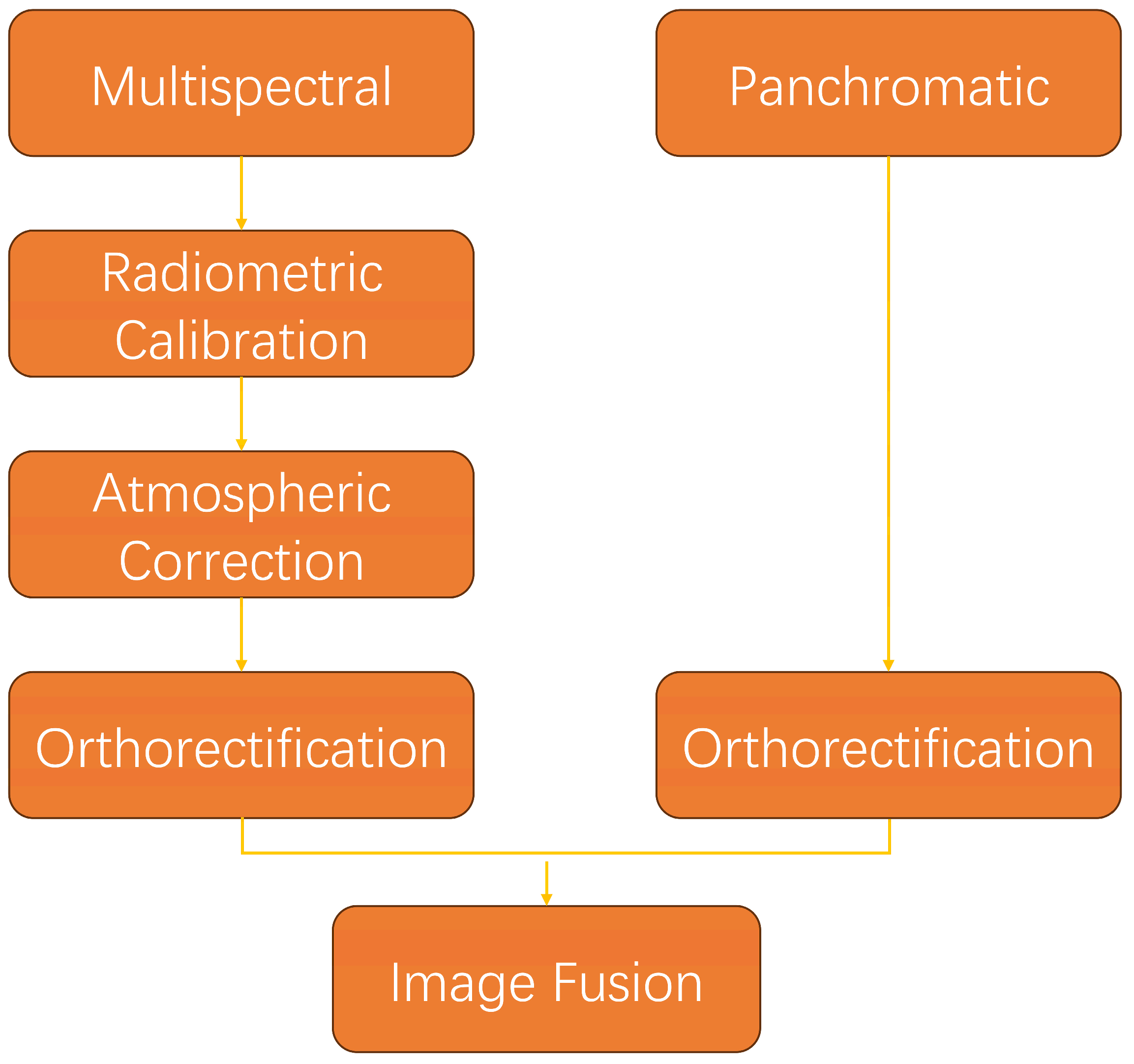
The proposed framework was developed and evaluated using GF-1 PMS2 imagery acquired over Chengdong, Chengzhong, and Chengxi Districts of Xining City, Qinghai Province. The developed technical framework encompassed data preprocessing, dataset construction, model selection, and model improvement for pixel-level binary semantic segmentation of bare rock and background [28,29]. Radiometric calibration, atmospheric correction, orthorectification, and image fusion were first performed on the GF-1 multispectral and panchromatic data to generate 2-m fused imagery for subsequent RGB image-patch construction. The fused remote-sensing imagery was cropped into non-overlapping 256 × 256-pixel patches using the Split Raster tool in ArcMap 10.8. For construction of the deep-learning dataset, the red, green, and blue visible bands were retained to form a true-color RGB representation, whereas the near-infrared band was not included in the network input. The resulting image patches were converted into three-channel RGB images and saved in JPEG format. Therefore, the actual network input was a 256 × 256 × 3 RGB image rather than the complete four-band multispectral image. Following geographic partitioning, the candidate patch pool was jointly screened by three researchers based on image validity, bare-rock occurrence, and the representation of typical background conditions. A total of 638 original patches were selected for the training–validation dataset, and 128 spatially separated original patches were selected as the internal test set, resulting in 766 original image–label pairs before data augmentation. These 638 patches were subsequently divided into 510 training patches and 128 validation patches according to the predefined spatial partition strategy. To further characterize the dataset at the patch level, the original patches were classified according to the presence of valid bare-rock pixels. A bare-rock-containing patch was defined as a patch containing at least one valid bare-rock pixel, whereas a background-only patch contained no valid bare-rock pixels. Before data augmentation, the training set contained 430 bare-rock-containing and 80 background-only patches, the validation set contained 111 bare-rock-containing and 17 background-only patches, and the internal test set contained 115 bare-rock-containing and 13 background-only patches. Representative background-only patches covered typical urban background scenes, including buildings, roads, vegetation, bare soil, water bodies, dry riverbeds, and shadowed areas. Pixel-level statistics were calculated separately for valid class labels and ignored pixels. In the final training set, background and bare-rock pixels accounted for 94.33% and 5.67% of the valid labeled pixels, respectively, corresponding to a class imbalance ratio of approximately 16.64:1. Pixels assigned a value of 255 represent ambiguous transition pixels along the manually delineated bare-rock boundaries. Specifically, the interior of each annotated bare-rock polygon was assigned to the bare-rock class, whereas a two-pixel-wide contour along the polygon boundary was assigned the ignore label (255). These narrow boundary regions were excluded because the exact class membership of pixels at the bare-rock–background transition could not always be reliably determined. Thus, label 255 was used to represent boundary uncertainty rather than to systematically exclude shadow-affected regions. Pixels labeled 255 were excluded from loss calculation during model training and were also excluded from all validation, internal-test, and external-test metric calculations; accordingly, only ground-truth pixels labeled as background or bare rock contributed to the quantitative evaluation. Relative to all ground-truth label pixels in each subset, ignored pixels accounted for 1.99%, 1.87%, 1.80%, and 3.01% of the training, validation, internal-test, and external-test sets, respectively. Before data augmentation, the original candidate patches were organized according to predefined geographic partitions, from which 510 training patches, 128 validation patches, and 128 internal-test patches were selected. The three subsets were established prior to data augmentation and maintained fixed throughout the subsequent experiments. Ultimately, using the DeepLabV3+ framework, the baseline configuration was selected by comparing four backbone networks and two optimizers. Drawing on recent improvements to DeepLabV3+ for complex remote-sensing segmentation tasks, including attention enhancement, large-kernel modeling, and transfer learning [30,31,32], the SE channel attention, SATM-based spatial attention, and RFB receptive-field enhancement modules were integrated to develop a bare-rock segmentation model for complex urban environments.

2.2.1. Image Preprocessing

(1)

To accommodate the different characteristics of GF-1 PMS2 multispectral and panchromatic data, a “separate preprocessing–fusion enhancement” workflow was adopted, as illustrated in Figure 1. Standardized processing, which includes radiometric calibration, atmospheric correction, orthorectification, and image fusion, was performed on the raw L1A data using ENVI 5.6.2 software to mitigate systematic errors and atmospheric interference. This processing generated a 2-m pan-sharpened multispectral raster that served as the source product for subsequent image-patch generation. The complete multispectral raster was not directly used as the network input; only its red, green, and blue visible bands were retained for the RGB-based deep-learning experiments.

(i)

Radiometric calibration converts the original digital number (DN) values into top-of-atmosphere radiance. The official GF-1 absolute calibration coefficients were applied to the original Level-1A multispectral bands. The DN values were converted to at-sensor radiance using the official GF-1 calibration coefficients, thereby reducing radiometric inconsistencies associated with sensor response and gain differences. This procedure provided standardized radiometric data for subsequent atmospheric correction.

(ii)

Atmospheric correction was performed using the built-in FLAASH module in ENVI 5.6.2 to reduce the effects of atmospheric scattering, gas absorption, aerosols, and water vapor on the remotely sensed signal and to estimate surface reflectance. The study area is located at approximately 36.7° N, and the imagery used for the internal experiments was acquired on 24 September 2024. According to the latitude–season guidance for the standard MODTRAN atmospheric profiles implemented in FLAASH, the Mid-Latitude Summer profile is specified for September acquisitions near the 40° N latitude band. Therefore, the Mid-Latitude Summer atmospheric profile was adopted for the atmospheric correction of the study-area imagery. Here, “Summer” refers to the name of the predefined MODTRAN atmospheric profile rather than to the calendar season of image acquisition. Other core parameters were set as follows: a rural aerosol model was used, with an initial visibility of 40 km and an aerosol elevation of 1.50 km; the MODTRAN spectral resolution was set to 5 cm⁻¹; adjacency-effect correction was enabled; and no aerosol inversion method was applied. Elevation information was derived from the mean elevation of the corresponding GMTED2010 region. The atmospheric correction parameters were matched to the image location and acquisition time to estimate surface reflectance, thereby reducing atmospheric effects and improving the spectral separability of rocks and vegetation.

(iii)

Orthorectification was performed to correct geometric distortions associated with terrain relief and satellite viewing geometry. Using the RPC model and the SRTM 30 m DEM in ENVI 5.6.2, the GF-1 multispectral and 2 m panchromatic images were orthorectified separately. The corrected imagery was projected to WGS 84/UTM Zone 47N and resampled using cubic convolution. The orthorectified imagery provided a consistent spatial reference for subsequent image fusion, patch generation, and sample annotation.

(iv)

Image fusion was performed to enhance the spatial resolution of the multispectral imagery using the high-resolution panchromatic image. In ENVI 5.6.2, the orthorectified multispectral imagery was first converted from band sequential (BSQ) to band interleaved by line (BIL) format. Both BSQ and BIL describe data-storage organization and do not alter pixel values, spectral information, or spatial resolution. The format conversion was used only as part of the ENVI preprocessing workflow before NNDiffuse pan-sharpening. Subsequently, the NNDiffuse pan sharpening algorithm was applied to fuse the 2 m panchromatic image with the preprocessed multispectral image, producing a fused raster with a spatial resolution of 2 m. The resulting fused raster was used as the source data for subsequent image-patch generation rather than being directly input into the deep-learning network. For the subsequent segmentation experiments, only the red, green, and blue visible bands of the pan-sharpened product were retained to generate RGB image patches, whereas the near-infrared band was excluded from the network input. Therefore, pan sharpening was treated as an image-preprocessing step for spatial enhancement and RGB image construction, and no generalized conclusion regarding full-multispectral spectral fidelity was made in this study.

(2)

In this study, the preprocessed fused images were cropped into non-overlapping 256 × 256-pixel patches using the Split Raster tool in ArcMap 10.8. The fused GF-1 imagery had a spatial resolution of 2 m, corresponding to a ground coverage of approximately 512 × 512 m for each 256 × 256-pixel patch. The complete study-area imagery produced a candidate patch pool larger than that required for the model experiments. Final experimental samples were therefore selected from spatially defined candidate regions according to image validity and the representation of bare-rock and background scenes. For geographic partitioning, four spatially adjacent candidate patches arranged in a 2 × 2 configuration were combined into a Spatial Group with an approximate ground extent of 1.024 × 1.024 km. Spatial Groups were used as the basic geographic units for assigning the training, validation, and internal-test regions. Each Spatial Group was associated with a single dataset partition, thereby preserving the geographic integrity of locally adjacent candidate patches. A minimum edge-to-edge separation threshold of 1000 m was established among the training, validation, and internal-test regions. Because the candidate patches were aligned to a regular 512-m geographic grid, the resulting minimum geographic separation was 1024 m. GIS-based distance measurements were performed in the WGS 84/UTM Zone 47N projected coordinate system. The minimum edge-to-edge distances were 1024 m for the training–validation, training–internal-test, and validation–internal-test pairs. Spatial Groups located within the inter-partition separation zones were reserved as geographic buffers and excluded from experimental sample selection. The spatial partitioning strategy and the distribution of candidate regions for internal and external datasets are illustrated in Figure 2. This visualization demonstrates the geographic separation among dataset subsets and the independent sampling region used for external evaluation. After spatial partitioning, the training, validation, and internal-test candidate regions contained 776, 155, and 156 candidate patches, respectively, as shown in Figure 2a. Following establishment of the geographic partitions, representative samples were selected within the corresponding training, validation, and internal-test candidate regions. Sample selection considered image validity, bare-rock occurrence, and representative background conditions. This procedure resulted in 510 original training patches, 128 validation patches, and 128 internal-test patches.

(3)

For construction of the deep-learning dataset, the red, green, and blue visible bands were selected from the fused GF-1 imagery to form a true-color RGB representation, whereas the near-infrared band was excluded from the current network input. For the 16-bit input imagery, each retained RGB channel was independently subjected to percentile-based intensity stretching. Specifically, the 1st and 99th percentiles were calculated from non-zero pixels in each channel, and pixel values between these limits were linearly mapped to the 8-bit range of 0–255, with values outside the limits clipped accordingly. After 8-bit conversion, fixed contrast and color-saturation enhancement factors of 1.3 and 1.2, respectively, were applied. The resulting RGB image patches were saved in JPEG format with a quality setting of 98. JPEG was retained as the image representation used consistently in the established RGB dataset construction, annotation, training, and evaluation pipeline. This format choice was made for consistency with the RGB processing workflow rather than for preservation of the complete quantitative radiometric information of the original multispectral raster. Pixel-level manual annotation was performed using LabelMe by one primary annotator and subsequently cross-checked by a second researcher. The pan-sharpened GF-1 imagery was used as the primary annotation reference, while high-resolution reference imagery accessed through the Ovital Map platform was used as auxiliary visual information for uncertain regions. The auxiliary imagery was used only for label interpretation and verification and was not used as network input. A two-pixel-wide contour along each manually delineated bare-rock boundary was assigned the ignore label 255 to represent ambiguous bare-rock–background transition pixels. The same annotation and label-verification protocol was applied to the internal and external datasets. At the patch level, the training subset contained 430 bare-rock-containing and 80 background-only patches, while the validation subset contained 111 bare-rock-containing and 17 background-only patches. The internal test set contained 115 bare-rock-containing and 13 background-only patches. Data augmentation was applied only to the 510 original training samples. Images and their corresponding semantic labels were synchronously transformed at a ratio of 1:1, producing 510 additional image–label pairs and increasing the training set to 1020 image–label pairs. The validation set and internal test set were not augmented, and each retained 128 original samples. Therefore, the final training, validation, and internal-test sets contained 1020, 128, and 128 image–label pairs, respectively. Geographic partitioning and final sample selection were completed before data augmentation. The augmentation operations included random scaling with a scale factor sampled from 0.25 to 2.0, aspect-ratio perturbation with a jitter factor of 0.3, horizontal flipping with a probability of 0.50, Gaussian blurring with a 5 × 5 kernel and a probability of 0.25, and random rotation within −10° to +10° with a probability of 0.25. HSV-based photometric perturbation was also applied to the RGB images, with hue, saturation, and value parameters set to 0.1, 0.7, and 0.3, respectively. Geometric transformations were synchronously applied to the RGB images and their corresponding masks, whereas photometric transformations were applied only to the RGB images. Random scaling, aspect-ratio perturbation, and HSV-based photometric perturbation were applied to each augmented training sample, corresponding to an application probability of 1.0. No random augmentation was applied to the validation, internal-test, or external-test sets.

2.2.2. Model Construction

This section describes the construction of the improved bare-rock segmentation model in three sequential steps: (1) backbone network selection, in which Xception, ResNet50, MobileNetV2, and MobileNetV3 were compared; (2) optimizer selection, in which SGD and Adam were evaluated; and (3) module integration, in which SE, SATM, and RFB were incorporated into the selected ResNet50 + Adam baseline.

(1)

Backbone Network Selection

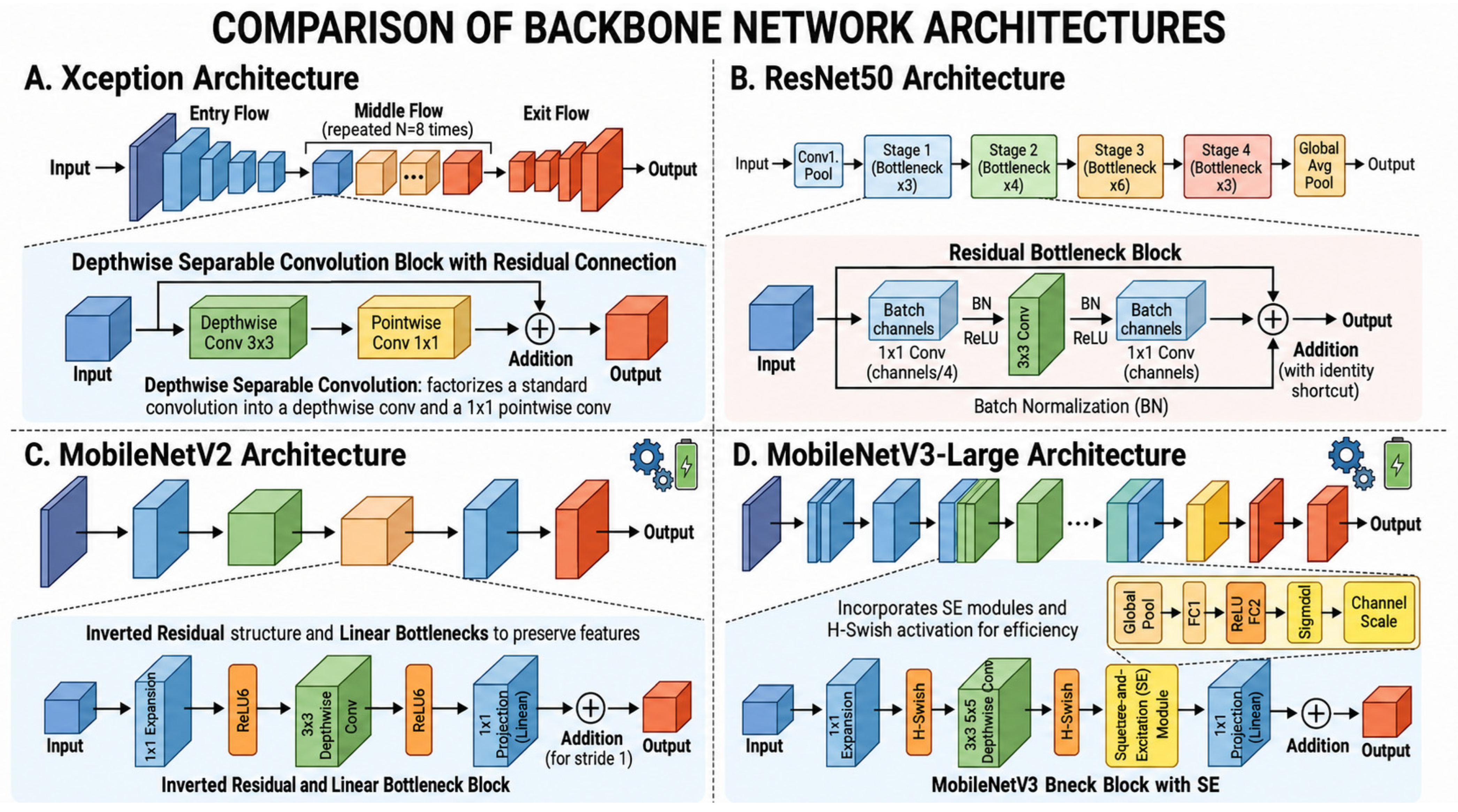
To select a suitable feature-extraction backbone for the binary semantic segmentation of bare rock and background in urban Xining, four backbone networks—Xception, ResNet50, MobileNetV2, and MobileNetV3—were evaluated, as illustrated in Figure 3. To ensure a fair comparison, all backbone networks were evaluated within the same DeepLabV3+ framework using the same dataset and a uniform input size of 256 × 256 pixels. Before being fed into the network, the RGB pixel values were converted to floating-point values and divided by 255, thereby scaling them from [0, 255] to [0, 1]. The backbone-selection experiments were conducted under a common SGD-based training configuration. The optimizer parameters and learning-rate scheduling settings were kept identical across the four backbone networks to isolate the effect of backbone architecture. Recent image-segmentation studies have shown that residual structures, edge-enhancement attention, spatial-pyramid context aggregation, and shape constraints can improve multi-scale feature representation and boundary delineation in complex images [33,34,35]. On this basis, performance comparison experiments were conducted to evaluate the feature representation capability and adaptability of different backbone networks to complex environments, ultimately determining the most suitable core backbone.

(i)

Analysis of Backbone Network Characteristics

ResNet50, a representative deep residual network, provides strong feature representation and stable deep-network training. Its residual connections facilitate gradient propagation during deep-network training and help alleviate network degradation. This architecture enables hierarchical extraction of color, texture, and contextual features from the three-channel RGB input, facilitating discrimination between bare rock and background objects such as buildings and vegetation in GF-1 imagery. Additionally, the bottleneck structure uses 1 × 1 convolutions for channel reduction and expansion, enabling deep feature extraction while limiting unnecessary computational redundancy [36].

Xception employs depthwise separable convolutions to reduce computational cost. Under the common experimental setting used in this study, Xception achieved lower bare-rock IoU and bare-rock F1-score than ResNet50. Therefore, ResNet50 was selected as the backbone for the subsequent experiments [37].

MobileNetV2 uses inverted residuals and linear bottleneck structures to reduce model complexity. Under the common experimental configuration used in this study, MobileNetV2 achieved a bare-rock IoU of 70.01% and a bare-rock F1-score of 82.36%, both lower than those of ResNet50. Therefore, ResNet50 was selected for the subsequent experiments [38].

MobileNetV3 incorporates inverted residual structures, lightweight attention mechanisms, and hardware-aware architecture design. Under the common experimental configuration used in this study, it achieved a bare-rock IoU of 67.38% and a bare-rock F1-score of 80.51%, both lower than the corresponding values obtained with ResNet50. Therefore, ResNet50 was retained for subsequent experiments [39].

(ii)

Performance Comparison and Backbone Selection

Using the same dataset, training parameters, and evaluation metrics, the four backbone networks were quantitatively compared for the binary semantic segmentation of bare rock and background. In this study, IoU, precision, and F1-score were calculated as class-specific metrics for the bare-rock class rather than as macro-averaged metrics over both classes. The results are summarized in

Table 1. Bare-rock segmentation performance of different backbone networks under the common SGD-based training configuration.

Backbone	IoU (%)	Precision (%)	F1-Score (%)
Xception	64.85	83.85	78.67
ResNet50	70.35	75.65	82.60
MobileNetV2	70.01	78.20	82.36
MobileNetV3	67.38	76.33	80.51

.

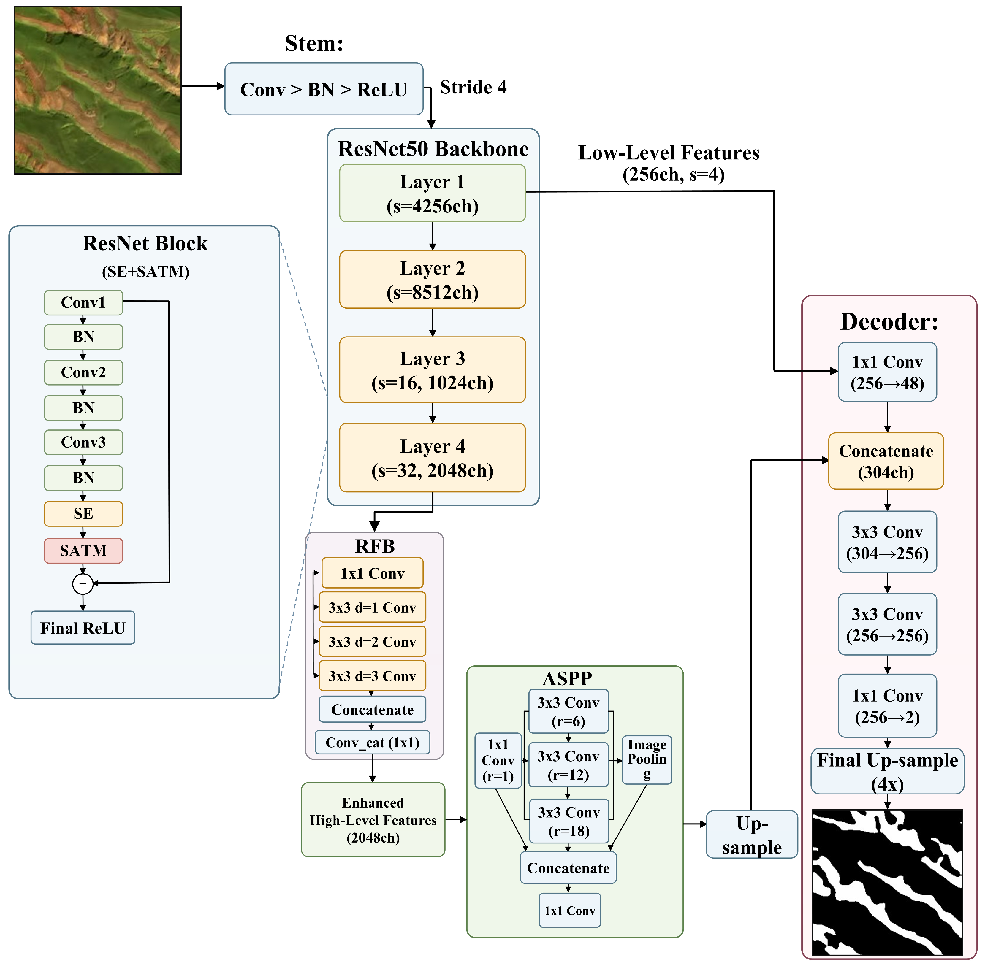
Among the four evaluated backbones, ResNet50 achieved the highest bare-rock IoU (70.35%) and bare-rock F1-score (82.60%). Its bare-rock IoU was 5.50, 0.34, and 2.97 percentage points higher than those of Xception, MobileNetV2, and MobileNetV3, respectively. In the backbone comparison, bare-rock IoU was used as the primary selection metric, with bare-rock precision and bare-rock F1-score considered as complementary metrics. Under the common experimental configuration, ResNet50 achieved higher bare-rock IoU and bare-rock F1-score than the other evaluated backbones. It was therefore selected as the backbone for the subsequent optimizer and module experiments. The low-level features used in the decoder are derived from the output of ResNet50 Layer1, with a spatial stride of 4 and 256 channels, forming multi-scale feature complementarity with high-level semantic features. The ResNet50 encoder used an output stride of 32, while the Layer1 low-level feature used by the decoder had a spatial stride of 4.

(2)

Optimizer Selection: SGD and Adam

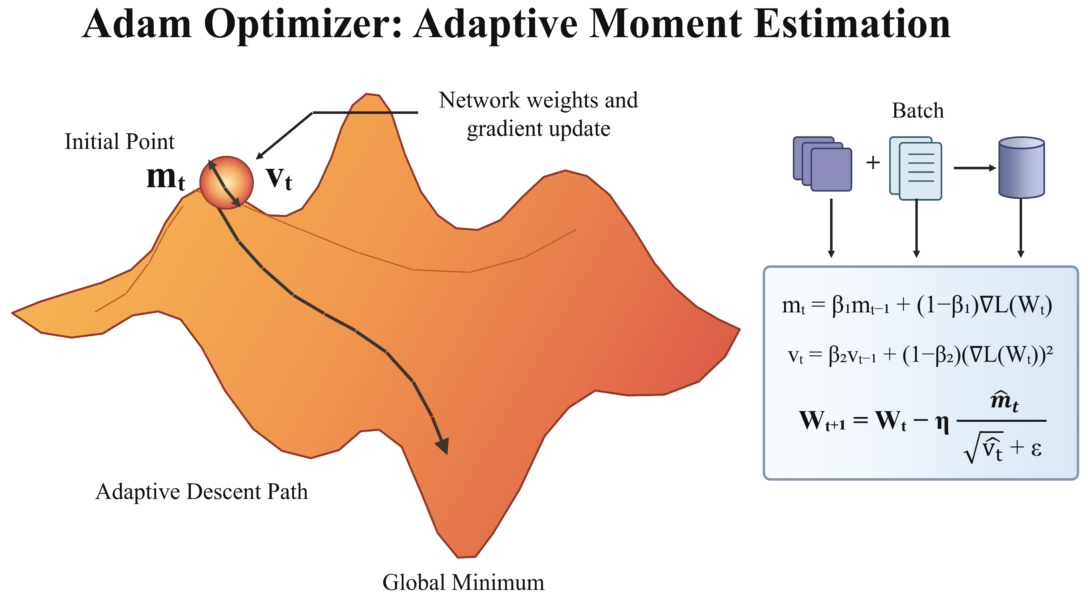
The urban scenes in the study area are complex, bare-rock targets are spatially scattered, and the sample distribution is imbalanced. In this study, Adam was evaluated against SGD for the ResNet50-based DeepLabV3+ baseline. The optimizer and the learning-rate schedule were treated as separate components of the training configuration. For the SGD configuration, the initial learning rate was set to 7 × 10⁻³, and the minimum learning rate was set to 7 × 10⁻⁵, corresponding to 1% of the initial learning rate. The momentum coefficient was set to 0.9, weight decay was set to 0, and Nesterov momentum was enabled. The SGD learning rate was dynamically adjusted using a cosine-based learning-rate schedule rather than being kept fixed throughout training. For Adam, ${{\displaystyle \beta }}_1$, ${{\displaystyle \beta }}_2$, epsilon, and weight decay were set to 0.9, 0.999, 1 × 10⁻⁸, and 1 × 10⁻⁵, respectively. Adam adaptively scales parameter-wise updates through first- and second-order moment estimates of the gradients, whereas the global learning rate during training is independently controlled by the learning-rate scheduling strategy.

Recent remote-sensing segmentation studies have demonstrated that feature fusion, multi-scale representation, and global-context modeling can improve target extraction in complex scenes [40,41,42]. Because optimizer-specific learning-rate settings were retained, this experiment should be interpreted as a comparison between the SGD-based and Adam-based training configurations rather than as a strictly isolated single-variable test of optimizer identity. The optimizer comparison conducted in this study was subsequently used to determine the training configuration adopted for the ResNet50 baseline.

The calculation formula for the first-order moment estimate is shown in Equation (1):

$${{\displaystyle m}}_t={{\displaystyle \beta }}_1\times {{\displaystyle m}}_{t-1}+\left(1-{{\displaystyle \beta }}_1\right)\times {{\displaystyle g}}_t$$

(1)

The calculation formula for the second-order moment estimate is shown in Equation (2):

$${{\displaystyle v}}_t={{\displaystyle \beta }}_2\times {{\displaystyle v}}_{t-1}+\left(1-{{\displaystyle \beta }}_2\right)\times {{\displaystyle g}}_t^2$$

(2)

The calculation formula for bias correction is shown in Equations (3) and (4):

$${{\displaystyle \widehat{m}}}_t={\displaystyle \frac{{{\displaystyle m}}_t}{1-{{\displaystyle \beta }}_1^t}}$$

(3)

$${{\displaystyle \widehat{v}}}_t={\displaystyle \frac{{{\displaystyle v}}_t}{1-{{\displaystyle \beta }}_2^t}}$$

(4)

The calculation formula for parameter update is shown in Equation (5):

$${{\displaystyle \theta }}_{t+1}={{\displaystyle \theta }}_t-\alpha \times {\displaystyle \frac{{{\displaystyle \widehat{m}}}_t}{\sqrt{{{\displaystyle \widehat{v}}}_t}+\epsilon }}$$

(5)

where: ${{\displaystyle g}}_t$ is the current gradient; ${{\displaystyle \beta }}_1$, ${{\displaystyle \beta }}_2$ are the momentum coefficients; $\alpha$ is the learning rate; $\epsilon$ is the smoothing factor. Under the evaluated training configuration, the Adam-based model showed favorable convergence behavior and higher reported bare-rock segmentation metrics than the tested SGD-based configuration. The structural diagram is presented in Figure 4.

(3)

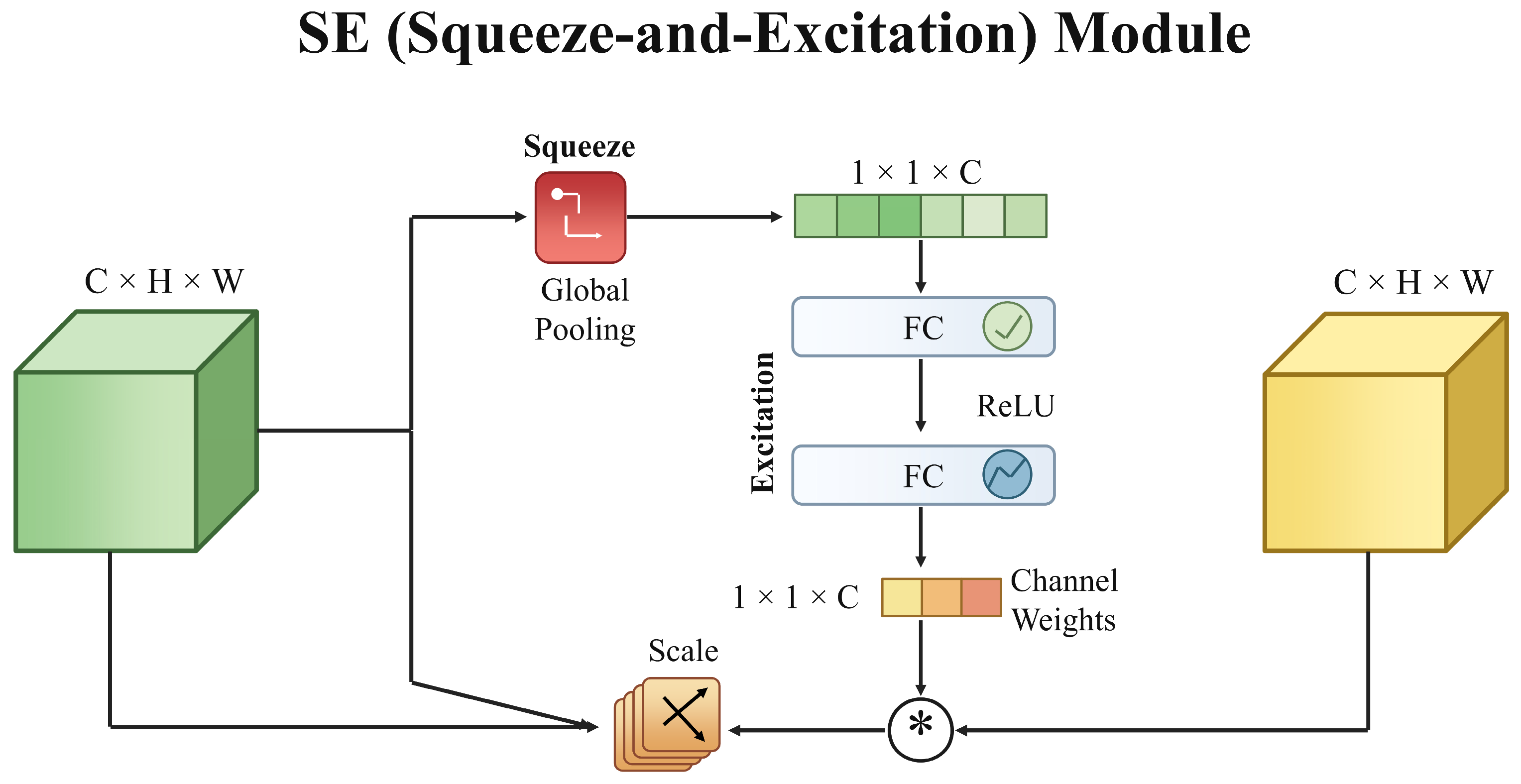
SE (Squeeze-and-Excitation) Channel Attention Module

High-resolution remote-sensing images contain diverse objects, including buildings, vegetation, roads, and water bodies. Complex backgrounds can obscure bare-rock features, while different deep feature channels contribute unequally to bare-rock segmentation. Channel and spatial attention mechanisms can adaptively assign feature weights and suppress irrelevant background responses [43,44,45,46]. In this study, the SE module models inter-channel dependencies and recalibrates deep feature responses to emphasize information relevant to bare-rock segmentation. Specifically, channel information is compressed through global average pooling. In this study, the SE channel attention module does not directly operate on the three-channel RGB input image but recalibrates the high-dimensional deep feature channels generated by the ResNet50 backbone. The SE module is embedded in all the Bottleneck residual blocks of the ResNet50 backbone network, placed after the conv3 convolution and BN layers. In this study, the SE channel-reduction ratio was set to 8 for the 256-, 512-, 1024-, and 2048-channel features corresponding to Layer1–Layer4. Accordingly, the intermediate channel dimensions of the SE excitation operation in Layer1, Layer2, Layer3, and Layer4 were 32, 64, 128, and 256, respectively. The SE and SATM modules were added only to the backbone network, while the structure and parameters of the native DeepLabV3+ ASPP module remained unchanged. In the decoder, the 256-channel low-level feature from ResNet50 Layer1 is first reduced to 48 channels using a 1 × 1 convolution. The 256-channel ASPP output is bilinearly upsampled to the same spatial resolution and concatenated with the 48-channel low-level feature, producing a 304-channel fused feature. Two successive 3 × 3 convolutional layers are then applied with channel transformations of 304 → 256 and 256 → 256, respectively, followed by dropout rates of 0.5 and 0.1. Finally, a 1 × 1 convolution maps the 256-channel feature to two output classes, and bilinear interpolation restores the prediction to the original input resolution. Specifically, the ASPP module consists of one 1 × 1 convolution branch, three 3 × 3 atrous-convolution branches with dilation rates of 6, 12, and 18, respectively, and one image-level pooling branch. Each branch outputs 256 channels. The five branch outputs are concatenated into a 1280-channel feature map and subsequently projected to 256 channels using a 1 × 1 convolution.

The calculation formula for obtaining the global feature description is shown in Equation (6):

$${{\displaystyle z}}_c={\displaystyle \frac{1}{H\times W}}{\displaystyle \sum _{i=1}^H{\displaystyle \sum _{j=1}^W{{\displaystyle x}}_c\left(i,j\right)}}$$

(6)

Subsequently, channel weights are learned through two fully connected layers, with the calculation formula shown in Equation (7):

$$s=\sigma \left({{\displaystyle W}}_2\times \delta \left({{\displaystyle W}}_1\times z\right)\right)$$

(7)

Finally, the learned weights are multiplied with the original features to achieve feature recalibration, as shown in Equation (8):

$${{\displaystyle \tilde{x}}}_c={{\displaystyle s}}_c\times {{\displaystyle x}}_c$$

(8)

where: ${{\displaystyle z}}_c$ is the global feature of the c-th channel; $\delta$ ReLU is the ReLU activation function; $\sigma$ is the Sigmoid activation function; ${{\displaystyle s}}_c$ is the channel weight. The SE module recalibrates the responses of high-dimensional feature channels according to learned channel weights, allowing channels associated with bare-rock color, texture, and semantic characteristics to receive greater emphasis. This mechanism is intended to improve the discriminative representation of bare-rock and background features. The structural diagram is presented in Figure 5.

(4)

SATM (Spatial Attention Module)

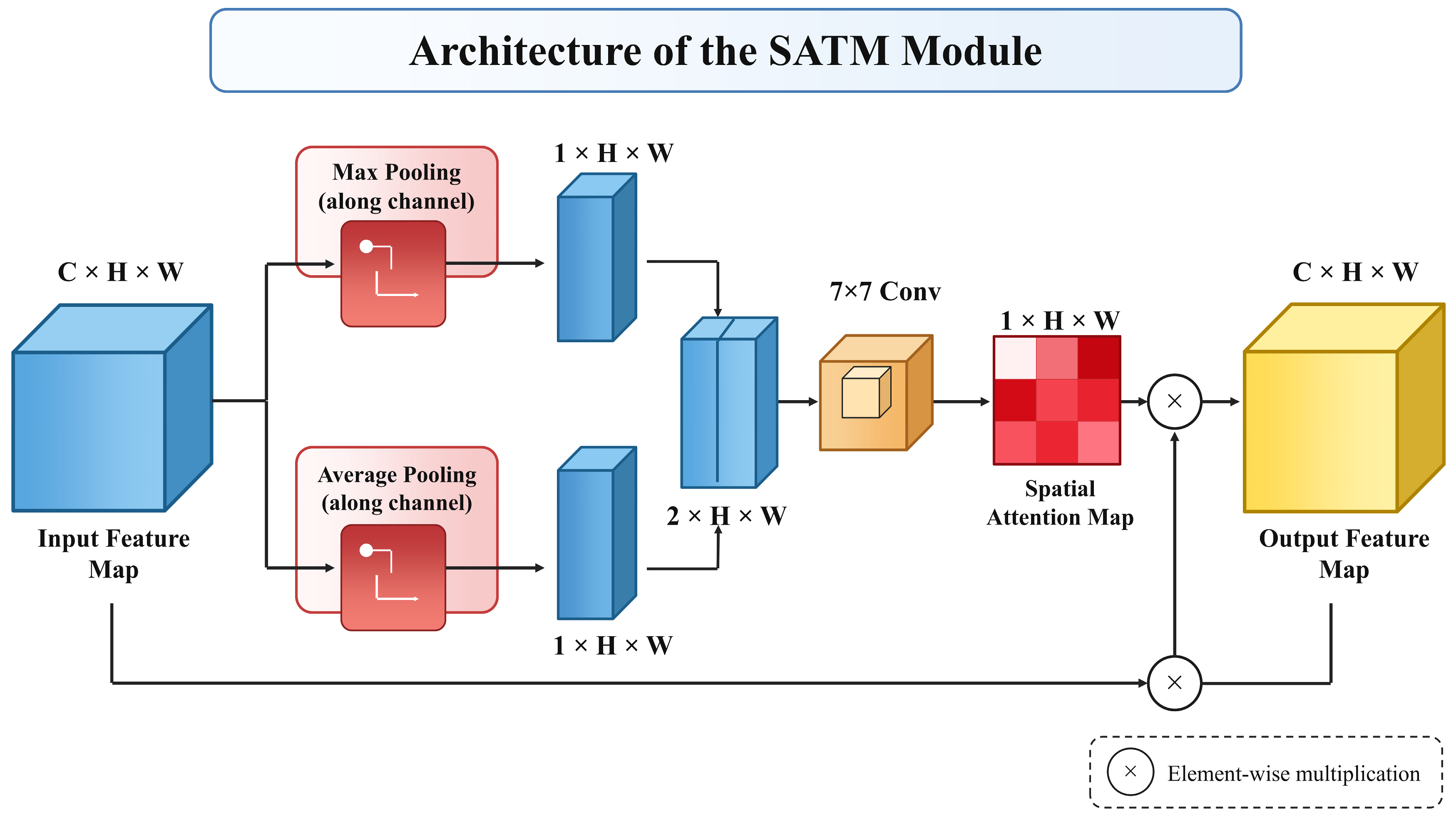
In the urban area of Xining, buildings are densely packed, and the terrain exhibits significant undulation. Consequently, bare-rock targets are frequently affected by shadows and occlusion, which complicate spatial localization and lead to ambiguous boundaries. The Spatial Attention Module (SATM) is designed to address these challenges by emphasizing the spatial locations of bare-rock targets, enhancing target-region features, and suppressing irrelevant background responses, thereby strengthening boundary-related spatial representation [47,48,49]. To avoid confusion with the Segment Anything Model (SAM), which is commonly abbreviated as SAM in remote-sensing studies [50], the abbreviation SATM is used throughout this manuscript for the spatial attention module. The SE and SATM modules are sequentially embedded after the conv3 convolution and BN layers of each ResNet50 Bottleneck block. The conv3–BN output is first recalibrated by the SE module in the channel dimension and subsequently processed by SATM for spatial recalibration. SATM uses channel-wise average pooling and maximum pooling, followed by a 7 × 7 convolution and Sigmoid activation to generate the spatial attention weights. The sequentially enhanced feature is then added to the residual shortcut branch and passed through ReLU activation. This design retains the complete three-layer convolution structure and shortcut branch of the original ResNet50 Bottleneck block without modifying its basic convolutional parameters, as illustrated in Equation (9):

$${{\displaystyle M}}_s\left(F\right)=\sigma \left({{\displaystyle f}}_{7\times 7}\left(\left[{{\displaystyle F}}_{avg}^s;{{\displaystyle F}}_{\max }^s\right]\right)\right)$$

(9)

The attention map is multiplied element-wise with the SE-recalibrated feature map entering the SATM to obtain spatially enhanced features, as shown in Equation (10):

$$F^{\prime }={{\displaystyle M}}_s\left(F\right)\otimes F$$

(10)

where: ${{\displaystyle F}}_{avg}^s$, ${{\displaystyle F}}_{\max }^s$ are the results of channel average pooling and max pooling, respectively; ${{\displaystyle f}}_{7\times 7}$ denotes a 7 × 7 convolution; $\sigma$ denotes the Sigmoid function; $\otimes$ denotes element-wise multiplication. In this study, the SATM module is used to enhance spatial feature representation and boundary-related responses in complex scenes. The structural diagram is presented in Figure 6.

(5)

RFB (Receptive Field Block)

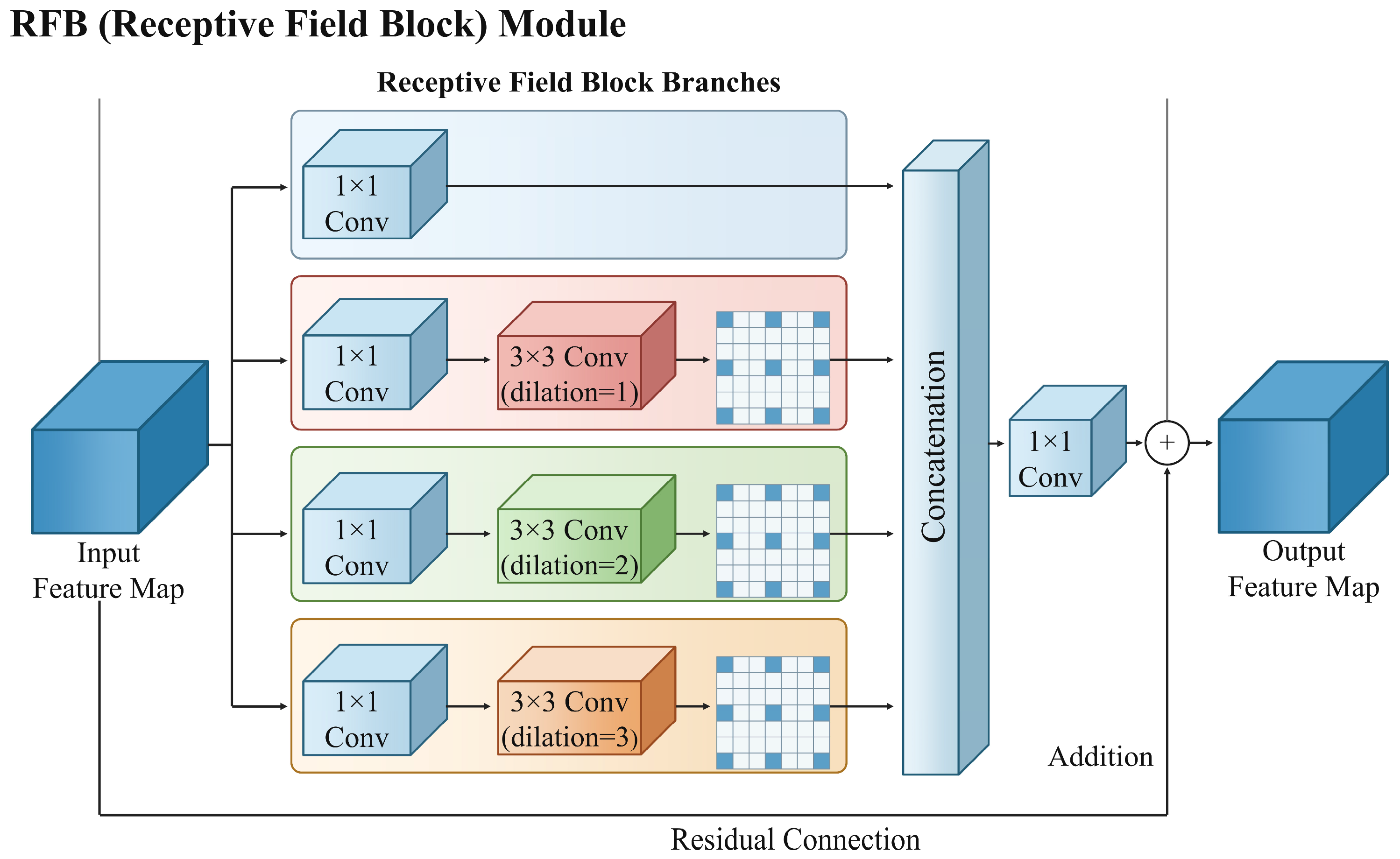
Rocks in the study area exhibit a multi-scale distribution, including extensive exposed bedrock and scattered small outcrops. Segmentation models with a single receptive field may struggle to capture targets at different scales. Previous studies have shown that multi-scale receptive-field and spatial-pyramid strategies can improve the extraction of targets with substantial scale variation [51,52,53]. In this study, the RFB constructs multi-scale receptive fields using parallel dilated-convolution branches with different dilation rates, expanding the effective receptive range without reducing feature-map resolution. The receptive field enhancement module (RFB) used in this study contains four parallel branches, with both the input and output dimensions set to 2048 channels, and employs dilation rates of 1, 2, and 3. To reduce the parameter overhead of multi-branch convolution on high-dimensional features, each branch first compresses the 2048-channel input feature to 256 channels through a 1 × 1 convolution. One branch directly retains the compressed feature, whereas the other three branches apply 3 × 3 dilated convolutions while maintaining 256 intermediate channels. The four branch outputs are concatenated into a 1024-channel feature map and subsequently projected back to 2048 channels through a 1 × 1 convolution. This module is inserted between the high-level output of the backbone network and the ASPP module to complement the multi-scale contextual representation provided by the native DeepLabV3+ ASPP. Initially, multi-scale feature branches are established using dilated convolutions with different dilation rates, as illustrated in Equation (11):

$${{\displaystyle B}}_k={{\displaystyle Conv}}_{3\times 3,}{{\displaystyle d}}_k\left({{\displaystyle Conv}}_{1\times 1}\left(F\right)\right)$$

(11)

The multi-branch features are concatenated and fused along the channel dimension, as shown in Equation (12):

$${{\displaystyle F}}_{RFB}={{\displaystyle Conv}}_{1\times 1}\left(Concat\left(B0,B1,B2,B3\right)\right)$$

(12)

Finally, enhanced features are output through a residual structure, as shown in Equation (13):

$$F^{\prime }={{\displaystyle F}}_{RFB}\oplus F$$

(13)

where: Subscript $K\in \left\{1,2,3\right\}$ in ${{\displaystyle B}}_k$ corresponds to three dilated branches with ${{\displaystyle d}}_k\in \left\{1,2,3\right\}$ calculated by Equation (11); ${{\displaystyle B}}_0$ denotes the single 1 × 1 convolution branch without dilated convolution. All four branches ${{\displaystyle B}}_0$, ${{\displaystyle B}}_1$, ${{\displaystyle B}}_2$, ${{\displaystyle B}}_3$ are concatenated in Equation (12); ${{\displaystyle d}}_k$ is the dilation rate of dilated convolution; $\oplus$ is element-wise addition for residual connection in Equation (13). The RFB module is designed to capture bare-rock features across multiple spatial scales and enhance multi-scale feature representation in complex terrains with diverse exposure patterns. The structural diagram is presented in Figure 7.

2.2.3. Evaluation Metrics

To evaluate the performance of the improved DeepLabV3+ model for the binary semantic segmentation of bare rock and background in urban Xining, bare-rock IoU, bare-rock precision, and bare-rock F1-score were used as the primary class-specific evaluation metrics during model development and ablation experiments. Bare-rock recall was additionally reported in the final cross-model comparison and external evaluation to explicitly characterize missed bare-rock detections. Considering the substantial class imbalance between background and bare-rock pixels, background IoU, mean Intersection over Union (mIoU), and Matthews Correlation Coefficient (MCC) were additionally calculated for the final model. Pixel-level confusion matrices were also used to characterize correct predictions, false-positive predictions, and false-negative predictions. For validation, internal-test, and external-test evaluations, only ground-truth pixels belonging to the valid background and bare-rock classes were included. Pixels assigned the ignore label (255) were excluded before constructing the confusion matrix and before calculating IoU, precision, recall, F1-score, mIoU, MCC, and other pixel-level evaluation statistics. Consequently, ignored pixels did not contribute to any reported quantitative evaluation metric, and all metrics were calculated from the same set of valid evaluation pixels. Model performance was evaluated from complementary perspectives, including bare-rock segmentation overlap, prediction reliability, two-class segmentation consistency, and confusion-matrix-based error characteristics. The definitions and calculation formulas for each metric are provided below:

(1)

Intersection over Union (IoU)

IoU is a commonly used metric for semantic segmentation that quantifies the overlap between a predicted region and its corresponding reference region. Its value ranges from 0 to 1, with higher values indicating greater overlap. For the binary semantic segmentation task considered in this study, IoU was calculated separately for the bare-rock and background classes. These values are referred to as bare-rock IoU and Background IoU, respectively. The bare-rock IoU and background IoU were calculated using Equation (14), and their arithmetic mean was used to calculate mIoU according to Equation (15):

$${{\displaystyle IoU}}_i={\displaystyle \frac{{{\displaystyle TP}}_i}{{{\displaystyle TP}}_i+{{\displaystyle FP}}_i+{{\displaystyle FN}}_i}}$$

(14)

$$mIoU={\displaystyle \frac{Io{U}_{rock}+Io{U}_{background}}{2}}$$

(15)

where: $i$ = 1 represents the bare-rock class, $i$ = 2 represents the background class; ${{\displaystyle TP}}_i$ (True Positive) refers to the number of true positive samples of the $i$-th class (the number of pixels that are truly of the $i$-th class and predicted as the $i$-th class); ${{\displaystyle FP}}_i$ (false positive) refers to the number of false positive samples of the $i$-th class (the number of pixels that are truly not of the $i$-th class but predicted as the $i$-th class); ${{\displaystyle FN}}_i$ (false negative) refers to the number of false negative samples of the i-th class (the number of pixels that are truly of the $i$-th class but predicted as not of the $i$-th class).

(2)

Precision

Precision measures the proportion of correctly predicted positive pixels among all pixels predicted as belonging to a specific class. Its value ranges from 0 to 1, with higher values indicating a lower proportion of false-positive predictions among the pixels predicted as that class. For the bare-rock class, higher precision consequently indicates greater reliability of predicted bare-rock pixels. The formula for calculating precision is presented in Equation (16):

$${{\displaystyle \mathrm{Pr}ecision}}_i={\displaystyle \frac{{{\displaystyle TP}}_i}{{{\displaystyle TP}}_i+{{\displaystyle FP}}_i}}$$

(16)

where: $i$ = 1 represents the bare-rock class, $i$ = 2 represents the background class; ${{\displaystyle TP}}_i$ (true positive) refers to the number of true positive samples of the $i$-th class (the number of pixels that are truly of the $i$-th class and predicted as the $i$-th class); ${{\displaystyle FP}}_i$ (false positive) refers to the number of false positive samples of the $i$-th class (the number of pixels that are truly not of the $i$-th class but predicted as the $i$-th class). This metric emphasizes the ratio of accurately predicted positive samples to the total number of predicted positive samples. Because precision can be influenced by class distribution, it should be interpreted together with recall.

(3)

F1-score

The F1-score is the harmonic mean of precision and recall and ranges from 0 to 1. Higher F1-score values indicate a better balance between the reliability of positive predictions and the completeness of target detection. In this study, the F1-score was used to provide a balanced class-specific assessment of bare-rock segmentation performance. The calculation formula for recall is presented in Equation (17), and the F1-score of the $i$-th class is given in Equation (18). The F1-score values reported in Table 1,

Table 2. Ablation results for different combinations of SE, SATM, and RFB modules based on the ResNet50 + Adam baseline. Values are reported as mean ± standard deviation across three independent training runs using random seeds 11, 22, and 33. The baseline configuration is shown in bold.

ResNet50	Adam	SE	SATM	RFB	IoU (%)	Precision (%)	F1-Score (%)
√	√	×	×	×	74.17 ± 0.82	84.05 ± 0.28	85.17 ± 0.54
√	√	×	×	√	78.43 ± 0.64	86.79 ± 0.97	87.91 ± 0.40
√	√	×	√	×	78.57 ± 0.52	87.00 ± 1.63	87.99 ± 0.32
√	√	√	×	×	78.60 ± 0.11	86.63 ± 0.21	88.02 ± 0.07
√	√	√	×	√	78.62 ± 0.50	86.88 ± 1.02	88.03 ± 0.31
√	√	×	√	√	78.80 ± 0.19	87.70 ± 0.28	88.14 ± 0.12
√	√	√	√	×	78.91 ± 0.33	87.85 ± 1.43	88.21 ± 0.21
√	√	√	√	√	79.36 ± 0.30	88.65 ± 0.55	88.49 ± 0.19

Note: √ indicates that the corresponding component is included, whereas × indicates that it is excluded. SE, squeeze-and-excitation; SATM, spatial attention module; RFB, receptive field block.

and

Table 3. Bare-rock segmentation performance of different deep-learning models on the internal test set.

Model	IoU (%)	Precision (%)	Recall (%)	F1-Score (%)
U-Net	76.06	90.92	82.31	86.40
SegFormer	69.82	75.80	89.83	82.22
PSPNet	62.67	85.73	69.97	77.05
HRNet	73.55	85.19	84.33	84.76
Modified DeepLabV3+	79.36	88.65	88.34	88.49

specifically refer to the F1-score of the bare-rock class.

$${{\displaystyle \mathrm{Re}call}}_i={\displaystyle \frac{{{\displaystyle TP}}_i}{{{\displaystyle TP}}_i+{{\displaystyle FN}}_i}}$$

(17)

$${{\displaystyle F1}}_i={\displaystyle \frac{2\times {{\displaystyle \mathrm{Pr}ecision}}_i\times {{\displaystyle \mathrm{Re}call}}_i}{{{\displaystyle \mathrm{Pr}ecision}}_i+{{\displaystyle \mathrm{Re}call}}_i}}$$

(18)

where: ${{\displaystyle \mathrm{Re}call}}_i$ is the recall of the $i$-th class (the proportion of samples truly belonging to the $i$-th class that are correctly predicted as the $i$-th class); ${{\displaystyle FN}}_i$ (false negative) is the number of false negative samples of the $i$-th class (the number of pixels truly belonging to the $i$-th class but predicted as non-$i$-th class); ${{\displaystyle F1}}_i$ is the F1-score of the $i$-th class.

(4)

Matthews Correlation Coefficient (MCC)

MCC was additionally adopted as a complementary balanced measure because it incorporates TP, TN, FP, and FN simultaneously and is informative for evaluating segmentation performance under substantial class imbalance. MCC ranges from −1 to 1, with values closer to 1 indicating stronger agreement between the predictions and the reference labels. The MCC is calculated using Equation (19):

$$MCC={\displaystyle \frac{TP\times TN-FP\times FN}{\sqrt{(TP+FP)(TP+FN)(TN+FP)(TN+FN)}}}$$

(19)

TN (True Negative) denotes the number of background pixels that are correctly predicted as background.

2.2.4. Experimental Configuration

The experiments were implemented using PyTorch 2.0.0 with CUDA 11.8 and Python 3.9.23, with PyCharm Community Edition 2020.1.3 used as the code development environment. All experiments were conducted on Windows 10 Professional Workstation Edition (22H2) with cuDNN 8.7.0 and an NVIDIA Quadro P2200 GPU with a total VRAM capacity of 5 GB. Owing to the limited GPU VRAM capacity, the input image resolution was set to 256 × 256 pixels. For the DeepLabV3+-based model-development experiments, optimizer-specific learning-rate settings were retained. For the SGD-based configuration used in the backbone-selection and optimizer-comparison experiments, the initial learning rate was set to 7 × 10^−3, and the minimum learning rate was set to 7 × 10⁻⁵, corresponding to 1% of the initial learning rate. The momentum coefficient was set to 0.9, weight decay was set to 0, and Nesterov momentum was enabled. The learning rate was dynamically adjusted using a cosine-based learning-rate schedule rather than remaining fixed throughout training. For the Adam-based ResNet50 baseline and subsequent module-ablation experiments, a two-stage training strategy was adopted. During epochs 1–15, the batch size was set to 8, and the initial learning rate was set to 1 × 10⁻⁴; during epochs 16–200, the batch size was set to 4, and the initial learning rate was set to 2 × 10⁻⁵. For Adam, ${{\displaystyle \beta }}_1$ = 0.9, ${{\displaystyle \beta }}_2$ = 0.999, epsilon = 1 × 10⁻⁸, and weight decay = 1 × 10⁻⁵. The stated initial learning rates were not held fixed throughout training; they served as the starting values of the corresponding training stages and were subsequently updated according to the cosine-based learning-rate schedule. To account for stochastic variation during model training, the module-ablation experiments and the convergence analyses of the original and modified DeepLabV3+ configurations were independently repeated three times using random seeds 11, 22, and 33. Across the three independent runs of each evaluated configuration, the dataset partition, configuration-specific optimizer parameters and learning-rate settings, standard pixel-wise cross-entropy loss without explicit class weighting, training epochs, and data-augmentation protocol were kept unchanged. In the original semantic masks, ignored boundary pixels were encoded as 255. During data loading, these pixels were remapped to the auxiliary index 2 (num classes = 2), and the cross-entropy loss used ignore index = 2; therefore, these pixels did not contribute to loss calculation or gradient optimization. For network-side resizing, RGB images were resized using bicubic interpolation, whereas semantic-label masks were resized using nearest-neighbor interpolation to preserve discrete class indices. Decoder feature maps and final output maps were resized using bilinear interpolation. No early-stopping mechanism was used; consequently, the patience parameter was not applicable. Training was performed for a maximum of 200 epochs, and the checkpoint corresponding to the minimum validation loss was retained as the best model for subsequent evaluation. The same fixed training, validation, and internal test sets were used for all runs. For these repeated DeepLabV3+-based model-development and ablation experiments, bare-rock IoU, bare-rock precision, and bare-rock F1-score were calculated on the same internal test set for each run, with pixels labeled 255 excluded before metric calculation. These three primary bare-rock class metrics for the repeated model-development experiments were therefore evaluated using the same valid ground-truth data and are reported as mean ± standard deviation across the three independent runs. For the final model, background IoU, mIoU, MCC, and pixel-level confusion-matrix statistics were additionally calculated for each of the three independent runs using the same valid evaluation pixels, and the corresponding metrics were summarized across the three runs. The mean represents the average model performance, whereas the standard deviation quantifies the run-to-run variability associated with stochastic training. For the cross-model comparison, architecture-specific optimization configurations were used for the comparative models rather than forcibly imposing identical optimization hyperparameters across different architectures. U-Net-ResNet101 was trained using the Adam optimizer with an initial learning rate of 1 × 10⁻⁴, zero weight decay, a warm-up cosine learning-rate schedule, and a batch size of 2. SegFormer-B5 used AdamW with an initial learning rate of 1 × 10⁻⁴, a weight decay of 1 × 10⁻², a warm-up cosine learning-rate schedule, and batch sizes of 8 and 4 in the two training stages, respectively. PSPNet-ResNet50-OS8-Aux used SGD with an initial learning rate of 1 × 10⁻², zero weight decay, a warm-up cosine learning-rate schedule, and batch sizes of 8 and 4 in the two training stages, respectively. HRNetV2-W48 used Adam with an initial learning rate of 5 × 10⁻⁴, zero weight decay, a warm-up cosine learning-rate schedule, and batch sizes of 16 and 8 in the two training stages, respectively. These architecture-specific configurations were based on the corresponding public GitHub implementations adopted in this study. Only the maximum number of training epochs was uniformly set to 200. No ImageNet-pretrained weights, segmentation-pretrained weights, or other external pretrained model weights were used; all models were trained from scratch. All models used the same fixed training, validation, and internal-test partitions, the same 256 × 256 RGB inputs, the same prepared training samples, and the same evaluation protocol. The standardized 1:1 data augmentation was applied only to the training data, while the validation and internal-test sets remained unaugmented.

For the computational comparison, all models were evaluated using FP32 precision with a 1 × 3 × 256 × 256 input on the same NVIDIA Quadro P2200 GPU. Model parameters were calculated from the instantiated network parameters; MACs were computed using THOP, and FLOPs were reported according to the convention that one multiply–accumulate operation corresponds to two floating-point operations (FLOPs = 2 × MACs). Model size was determined from the serialized FP32 state dictionary, and inference time was measured with a batch size of 1 on the same GPU. Peak GPU memory consumption was not recorded during the computational benchmarking; consequently, model-specific GPU memory efficiency was not quantitatively evaluated in this study. The reported 5 GB VRAM refers to the total memory capacity of the NVIDIA Quadro P2200 GPU rather than the memory consumption of any individual model.

Considering the substantial pixel-level class imbalance between background and bare rock, an additional loss-function sensitivity experiment was conducted on the final ResNet50 + Adam + SE + SATM + RFB configuration. In addition to the standard cross-entropy loss used in the original model-development experiments, weighted cross-entropy, focal loss, and a combined cross-entropy–Dice loss were evaluated. To isolate the effect of the loss function, the network architecture, dataset partitions, optimizer, learning-rate schedule, batch sizes, training duration, data-augmentation strategy, and evaluation protocol were kept unchanged, and the random seed was fixed at 11 for the supplementary experiments. For weighted cross-entropy, the background and bare-rock class weights were set to 0.53 and 8.82, respectively, to increase the contribution of the minority bare-rock class during optimization. The experimental hardware parameters are shown in

Table 4. Experimental hardware parameters.

Hardware Component	Specification
Workstation	Lenovo workstation (Lenovo Group Limited, Beijing, China)
CPU	Intel Core i7-9700 CPU @ 3.00 GHz
Clock Frequency	3.00 GHz
GPU	NVIDIA Quadro P2200 (Professional Computing GPU)
GPU VRAM Capacity	5 GB
RAM (System Memory)	32.0 GB

.

3. Results

3.1. Ablation Experiment Results of the Improved DeepLabV3+ Model

To assess the contributions of the ResNet50 backbone, SE channel attention, SATM-based spatial attention, and RFB receptive-field enhancement to bare-rock segmentation performance, systematic ablation experiments were conducted using the ResNet50 + Adam baseline [54]. The contributions of the individual modules and their combinations were quantified through incremental ablation experiments. The schematic diagram of the improved model structure is presented in Figure 8.

(1)

As the backbone network, ResNet50 effectively mitigates the vanishing gradient problem in deep networks through its residual connection architecture. Its bottleneck design facilitates deep feature extraction while regulating the number of parameters, thereby enhancing model stability during training. Its deep feature-representation capability provided the baseline for subsequent module integration and supported discrimination between bare rock and background. Under this configuration, the bare-rock IoU was 70.35%, the bare-rock precision was 75.65%, and the bare-rock F1-score was 82.60%.

(2)

Based on the ResNet50 backbone network, the Adam-based training configuration was evaluated against the SGD-based configuration used in the preceding experiment. The Adam optimizer integrates the benefits of momentum gradient descent with adaptive parameter updates. By computing first-order and second-order moment estimates of the gradient and applying bias correction, it dynamically adjusts the parameter update magnitude during optimization. Under the reported experimental setting, the ResNet50 + Adam configuration achieved a bare-rock IoU of 74.17%, a bare-rock precision of 84.05%, and a bare-rock F1-score of 85.17%, compared with 70.35%, 75.65%, and 82.60%, respectively, for the tested ResNet50 + SGD configuration.

(3)

The SE module uses global average pooling and fully connected layers to learn channel weights and recalibrate deep feature responses. This mechanism emphasizes feature channels associated with bare-rock color, texture, boundary, and semantic information and is intended to improve the discriminative representation of bare-rock and background features. After the SE module was incorporated into the ResNet50 + Adam baseline, the mean bare-rock IoU, bare-rock precision, and bare-rock F1-score reached 78.60 ± 0.11%, 86.63 ± 0.21%, and 88.02 ± 0.07%, respectively. These results indicate higher mean values for all three reported bare-rock class metrics relative to the ResNet50 + Adam baseline under the evaluated experimental setting.

(4)

The SATM-based spatial attention module emphasizes the spatial locations of bare-rock targets by generating spatial attention maps that enhance edge detail features. By integrating spatial information from channel average pooling and max pooling, the learned attention map emphasizes spatially informative regions and suppresses irrelevant background responses. This mechanism enhances the representation of bare-rock boundaries in complex scenes, including regions affected by building shadows and topographic variation. In fine-grained segmentation tasks, the SATM module enhances the representation of boundary-related spatial features between bare rock and background. Under the evaluated experimental setting, the SE + SATM configuration achieved a mean bare-rock IoU of 78.91 ± 0.33%, a mean bare-rock precision of 87.85 ± 1.43%, and a mean bare-rock F1-score of 88.21 ± 0.21%.

(5)

The RFB receptive field enhancement module constructs a multi-scale receptive field through multi-branch dilated convolutions with varying dilation rates, thereby expanding the model’s spatial perception range. To address the multi-scale distribution of bare-rock targets in urban Xining, ranging from scattered outcrops to extensive exposed bedrock, the RFB captures feature information at different spatial scales. Compared with the SE + SATM configuration without RFB, adding RFB changed the mean bare-rock IoU from 78.91 ± 0.33% to 79.36 ± 0.30%, the mean bare-rock precision from 87.85 ± 1.43% to 88.65 ± 0.55%, and the mean bare-rock F1-score from 88.21 ± 0.21% to 88.49 ± 0.19%. These results indicate a modest positive change after introducing RFB. Considering the relatively small magnitude of the improvement together with the observed run-to-run variability, the contribution of RFB is conservatively interpreted as supplementary optimization for multi-scale feature representation rather than as a definitive or statistically significant improvement.

(6)

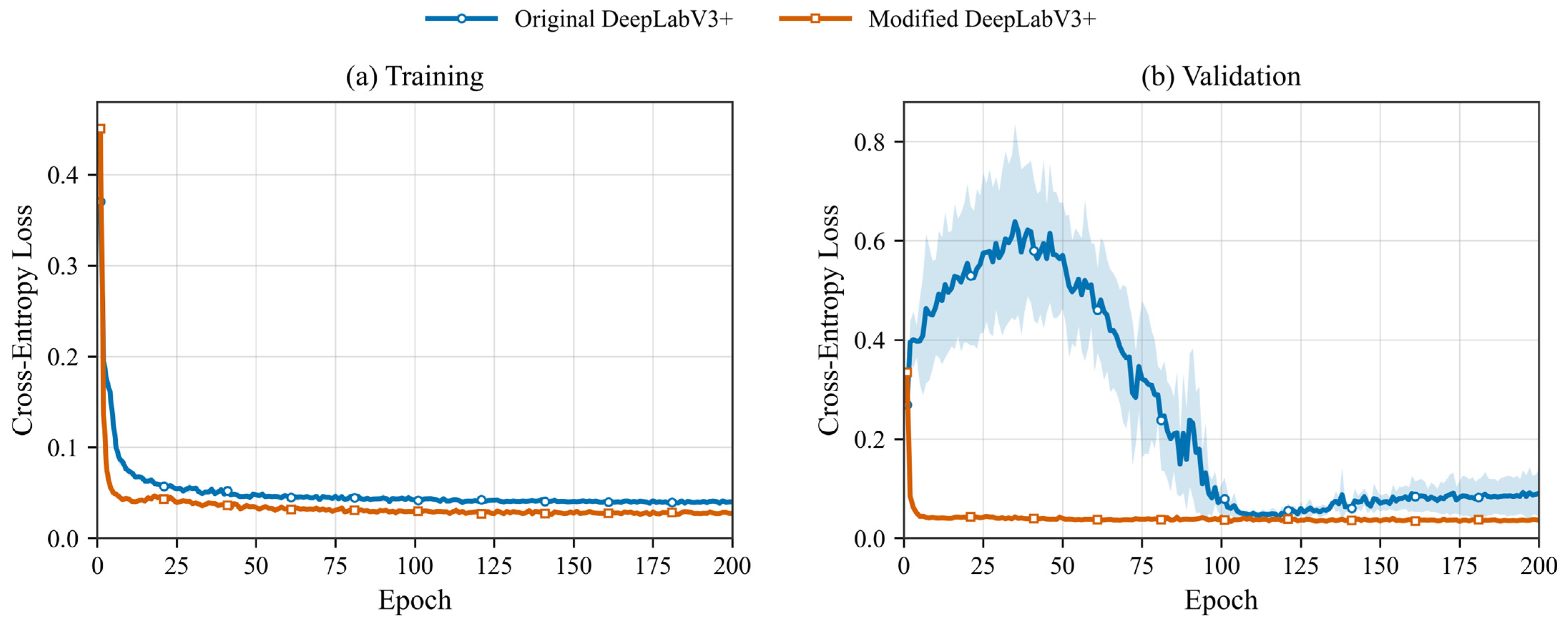
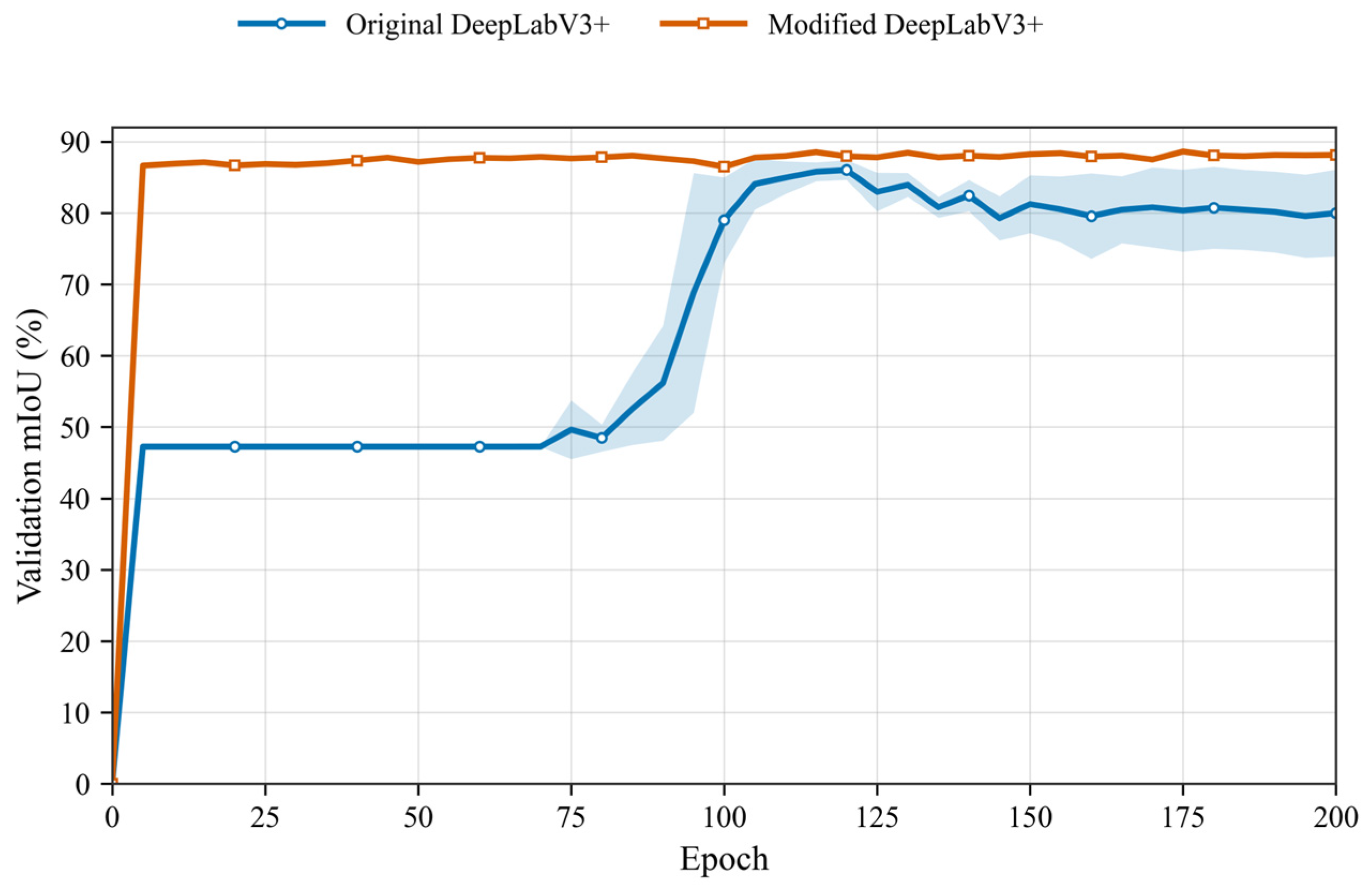
The final configuration combines ResNet50, Adam, SE, SATM, and RFB to provide backbone feature extraction, adaptive optimization, channel recalibration, spatial attention, and multi-scale feature modeling within a unified DeepLabV3+ framework. The ablation results indicate that configurations involving SE and SATM were associated with larger mean changes in the reported segmentation metrics, whereas the additional inclusion of RFB produced a smaller incremental change. To compare the training behavior of the original and modified configurations, their training and validation loss curves are shown in Figure 9, and the validation-set mIoU curves are shown in Figure 10. Both configurations were independently trained three times using random seeds 11, 22, and 33. The solid curves represent the mean values across the three independent runs, whereas the shaded regions indicate ±1 standard deviation. As shown in Figure 9, the original DeepLabV3+ configuration exhibited greater fluctuations in validation loss, whereas the modified configuration showed a smoother decrease in training loss and a more stable validation-loss trajectory. Figure 10 further shows that the modified configuration maintained higher mean validation mIoU values during the later stages of training. Together, these convergence curves characterize the optimization behavior and run-to-run variability of the two configurations under the evaluated experimental setting.

Experimental results are presented in Table 2. The evaluated class-specific metrics were bare-rock IoU, bare-rock precision, and bare-rock F1-score. Each ablation configuration was independently trained three times using random seeds 11, 22, and 33 under the same experimental settings. The results in Table 2 are reported as mean ± standard deviation across the three independent runs. Compared with the original DeepLabV3+ configuration (Xception + SGD), the final improved model showed higher reported values of bare-rock IoU, bare-rock precision, and bare-rock F1-score under the evaluated experimental setting.

(7)

To further examine the influence of class imbalance on the final model, supplementary loss-function sensitivity experiments were performed using the complete ResNet50 + Adam + SE + SATM + RFB configuration. Under the fixed-seed supplementary setting, weighted cross-entropy produced a bare-rock IoU of 58.39%, a bare-rock precision of 58.91%, and a bare-rock F1-score of 73.73%. Although increasing the contribution of the minority bare-rock class was intended to mitigate class imbalance, the substantial decreases in bare-rock IoU and precision suggest that stronger class weighting was associated with increased false-positive bare-rock predictions under this supplementary setting. Focal loss achieved a bare-rock IoU of 78.91%, a bare-rock precision of 86.07%, and a bare-rock F1-score of 88.22%, whereas the combined CE + Dice loss achieved a bare-rock IoU of 78.75%, a bare-rock precision of 89.42%, and a bare-rock F1-score of 88.11%, respectively. These two alternative losses maintained relatively high bare-rock segmentation performance but did not show a clear overall improvement over the standard cross-entropy results reported for the final model in Table 2. Taken together, the supplementary experiments indicate that stronger imbalance-oriented loss formulations did not necessarily improve overall bare-rock segmentation performance under the present dataset and training configuration. Under the evaluated configuration, standard cross-entropy provided the best overall balance among the loss functions tested in this supplementary experiment and was therefore retained for the final model.

(8)

To provide a more complete evaluation under the highly imbalanced rock–background distribution, additional metrics were calculated for the final model from the pixel-level confusion matrices of the three independent runs. The proposed model achieved a mean background IoU of 98.95 ± 0.02%, a mean mIoU of 89.15 ± 0.16%, and a mean MCC of 0.8796 ± 0.0020. These results indicate that the model maintained high segmentation agreement for both background and bare-rock classes under the evaluated setting. The mean normalized confusion-matrix statistics across the three independent runs showed that 99.48% of background pixels were correctly classified as background, whereas 0.52% were misclassified as bare rock. For the bare-rock class, 88.34% of pixels were correctly classified, whereas 11.66% were misclassified as background. These results further characterize the false-positive and false-negative behavior of the final model.

3.2. Comparison of Network Models

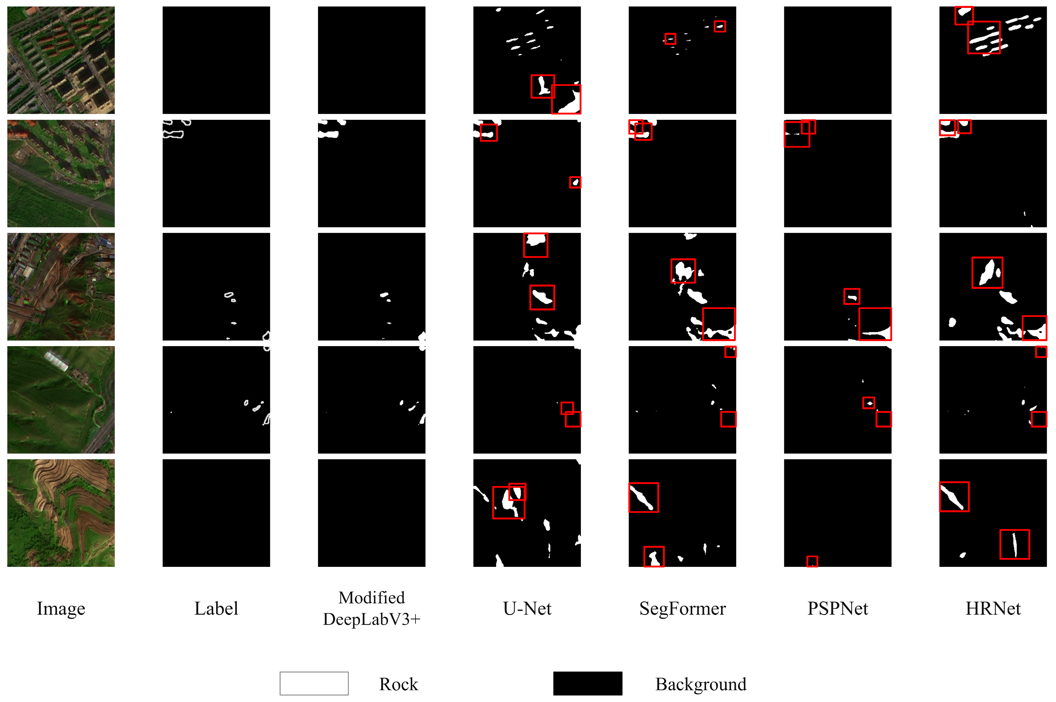
The comparative experiments were implemented using PyTorch 2.0.0 with CUDA 11.8 and Python 3.9.23 on a Windows 10 workstation equipped with an Intel i7-9700 CPU, 32 GB of RAM, and an NVIDIA Quadro P2200 GPU with a total VRAM capacity of 5 GB. To provide a controlled and reproducible cross-model comparison, U-Net with a ResNet101 encoder (U-Net-ResNet101), SegFormer-B5 with the MiT-B5 backbone, PSPNet with a ResNet50 backbone using output stride 8 and an auxiliary head (PSPNet-ResNet50-OS8-Aux), HRNetV2-W48, and the proposed modified DeepLabV3+ model used the same preprocessed GF-1 imagery, the same bare-rock annotation criteria, the same fixed dataset partitions consisting of 1020 training samples, 128 validation samples, and 128 internal-test samples, and the same 256 × 256 RGB input size. The 1:1 data-augmentation scheme was applied only to the training data, whereas the validation and internal-test sets remained unaugmented. Because different segmentation architectures have different optimization characteristics, identical optimization hyperparameters were not forcibly imposed on all models. Instead, U-Net-ResNet101, SegFormer-B5, PSPNet-ResNet50-OS8-Aux, and HRNetV2-W48 were trained using their respective architecture-specific optimization configurations, including model-specific optimizer, learning rate, weight decay, scheduler, and batch-size settings. Only the maximum training duration was standardized to 200 epochs to provide a comparable training budget. No ImageNet-pretrained or other external pretrained weights were used for any of the compared architectures. All models were evaluated on the same 128 internal test samples using the same set of bare-rock class-specific metrics. To evaluate the proposed model for the binary semantic segmentation of bare rock and background, it was compared with U-Net, SegFormer, PSPNet, and HRNet on the same internal test set. The comparison focused on bare-rock IoU, bare-rock precision, bare-rock recall, and rare-rock F1-score. The qualitative segmentation results are presented in Figure 11.

(1)

Segmentation Performance Analysis

As shown in Table 3, the proposed model achieved the highest bare-rock IoU (79.36%) and bare-rock F1-score (88.49%) among the evaluated models, whereas U-Net achieved the highest bare-rock precision (90.92%, compared with 88.65% for the proposed model). SegFormer achieved the highest bare-rock recall (89.83%), followed by the proposed model (88.34%). These results indicate that the comparative advantage of the proposed model is primarily reflected in segmentation overlap and the overall balance between precision and recall, rather than in maximizing either precision or recall individually.

Bare-rock IoU: The proposed model achieved a bare-rock IoU of 79.36%, which was 3.30, 9.54, 16.69, and 5.81 percentage points higher than those of U-Net, SegFormer, PSPNet, and HRNet, respectively. These results are consistent with the segmentation improvements observed in the preceding ablation experiments after the ResNet50 + Adam baseline and the SE, SATM, and RFB modules were introduced.

Bare-rock precision: The proposed model achieved a bare-rock precision of 88.65%, which was lower than that of U-Net (90.92%) but higher than those of SegFormer (75.80%), PSPNet (85.73%), and HRNet (85.19%). Therefore, U-Net exhibited a lower false-positive tendency for bare-rock predictions on the internal test set.

Bare-rock recall: SegFormer achieved the highest bare-rock recall of 89.83%, followed by the proposed model at 88.34%, HRNet at 84.33%, U-Net at 82.31%, and PSPNet at 69.97%. Although SegFormer achieved a slightly higher recall than the proposed model, its bare-rock precision was substantially lower (75.80% versus 88.65%), indicating a greater tendency to classify background pixels as bare rock. In contrast, the proposed model maintained a more balanced relationship between precision and recall, with values of 88.65% and 88.34%, respectively.

Bare-rock F1-score: The proposed model achieved a bare-rock F1-score of 88.49%, which was 2.09, 6.27, 11.44, and 3.73 percentage points higher than those of U-Net, SegFormer, PSPNet, and HRNet, respectively. This result indicates a favorable balance between bare-rock precision and recall under the reported experimental setting.

Besides segmentation performance, the computational complexity and inference efficiency of different models were further evaluated, and the results are summarized in

Table 5. Computational complexity and inference efficiency comparison of different deep-learning models on the internal test set.

Model	Parameters (M)	MACs (G)	FLOPs (G)	Model Size (MiB)	Inference Time (ms)
U-Net	62.92	27.89	55.78	240.64	32.88
SegFormer	84.59	24.94	49.88	323.07	60.55
PSPNet	49.07	48.64	97.28	187.52	43.94
HRNet	65.85	23.46	46.92	252.14	40.30
Modified DeepLabV3+	57.60	12.37	24.74	220.22	24.36

Note: Inference time was measured for processing one 256 × 256 RGB image patch with a batch size of 1 on an NVIDIA Quadro P2200 GPU.

.

In terms of computational complexity and inference efficiency, the proposed modified DeepLabV3+ model contains 57.60 M parameters and requires 12.37 GMACs and 24.74 GFLOPs for a 256 × 256 RGB input. Its serialized FP32 model size is 220.22 MiB, and its average inference time is 24.36 ms per patch on the NVIDIA Quadro P2200 GPU. Among the evaluated models, the proposed model achieved the lowest MACs, FLOPs, and inference time under the evaluated hardware setting. These results indicate that the introduced attention and multi-scale feature enhancement modules improved segmentation performance while maintaining a favorable balance between computational cost and efficiency. However, the proposed model does not have the smallest parameter count or model size, indicating a trade-off between feature representation capability and computational complexity. Combined with the highest bare-rock IoU and bare-rock F1-score among the evaluated models, these results indicate a favorable trade-off between segmentation performance and inference efficiency under the evaluated hardware setting.

(2)

Full-Area Prediction Visualization

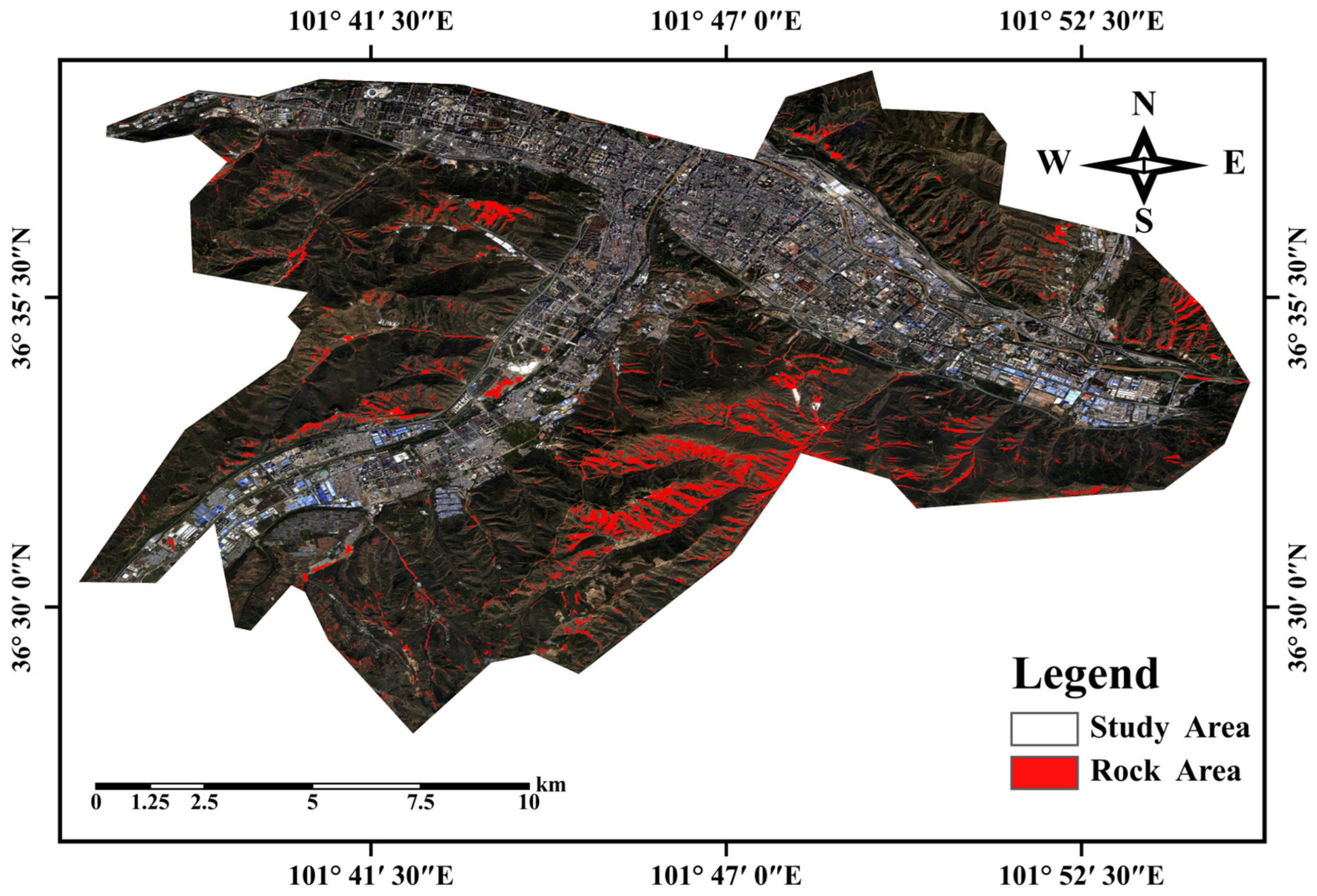
The trained model was applied to GF-1 imagery covering the entire study area (Chengdong, Chengzhong, and Chengxi Districts) to generate the bare-rock segmentation map shown in Figure 12. The full-area prediction exhibits the spatial distribution of model-identified bare-rock regions across urban backgrounds containing buildings, vegetation, roads, and shadow-affected areas. However, exhaustive pixel-level reference labels are not available for the complete study-area scene. Therefore, Figure 11 is presented only as a qualitative visualization of full-area predictions and is not used as independent evidence of segmentation accuracy.

3.3. External Evaluation in an Adjacent Region

To obtain preliminary evidence regarding the transferability of the proposed model beyond the original study area, Huangzhong District of Xining City, which is geographically adjacent to the core study area and shares related plateau river-valley environmental conditions, was selected as the external evaluation area. The cloud cover and snow cover of the imagery were both 0%, and the same preprocessing workflow, including radiometric calibration, atmospheric correction, orthorectification, and image fusion, was applied to the external imagery. During external sample selection, a 1.024-km geographic separation buffer was established along the boundary between the core study area and Huangzhong District. External-test candidate patches were selected from areas of Huangzhong District beyond this buffer. Candidate patches located within the potential overlap extent of the two GF-1 scenes or along invalid image edges were also excluded. The spatial relationship between the core study area and the Huangzhong external candidate region is shown in Figure 2b. A total of 128 non-overlapping 256 × 256-pixel patches were subsequently selected to construct the external test set. The external test set contained 119 bare-rock-containing patches and 9 representative background-only patches. Background-only patches contained no valid bare-rock pixels and were included to improve the representation of background-dominated scenes. Sample selection was based on the reference labels and representative scene characteristics and was independent of model prediction results. The external test set was fixed before model evaluation. The model weights obtained from the original study area were directly used for external inference without retraining, fine-tuning, or parameter adjustment. To provide a comparative assessment of external transferability, U-Net, which showed the strongest overall baseline performance in terms of bare-rock IoU and bare-rock F1-score in the internal model comparison, was additionally evaluated on exactly the same 128 external-test patches. The trained U-Net model was likewise directly applied to the external test set without retraining, fine-tuning, or parameter adjustment. The same external samples, preprocessing procedure, label-handling strategy, and evaluation protocol were used for both models.

Consistent with the internal evaluation protocol, pixels labeled 255 were excluded before metric calculation in the external test set. These ignored pixels accounted for 3.01% of all external-test label pixels. Consistent with the internal evaluation protocol, bare-rock IoU, bare-rock precision, bare-rock recall, and bare-rock F1-score were calculated as class-specific metrics for the bare-rock class. On the Huangzhong external test set, the proposed model achieved a bare-rock IoU of 81.29%, a bare-rock precision of 91.80%, a bare-rock recall of 87.66%, and a bare-rock F1-score of 89.68%. Under the same external evaluation conditions, U-Net achieved a bare-rock IoU of 76.84%, a bare-rock precision of 91.95%, a bare-rock recall of 82.39%, and a bare-rock F1-score of 86.91%. Compared with U-Net, the proposed model achieved increases of 4.45, 5.27, and 2.77 percentage points in bare-rock IoU, bare-rock recall, and bare-rock F1-score, respectively, while its bare-rock precision was 0.15 percentage points lower. When both models were directly applied to the same external dataset without retraining or parameter adjustment, the proposed model retained higher bare-rock IoU, bare-rock recall, and bare-rock F1-score, whereas U-Net achieved a marginally higher bare-rock precision. These results provide preliminary comparative evidence that the proposed model retained favorable bare-rock segmentation performance and its relative advantage in bare-rock IoU, bare-rock recall, and bare-rock F1-score when directly applied to the adjacent Huangzhong District. The higher external bare-rock IoU, bare-rock precision, and bare-rock F1-score may partly reflect differences in landscape composition and target characteristics between the two study areas. In northern Huangzhong District, bare-rock outcrops are generally larger, more continuous, and more widely distributed, with comparatively less interference from artificial buildings and dense vegetation. In contrast, the core urban study area contains denser building clusters and more fragmented bare-rock targets, resulting in stronger spectral confusion and shadow-occlusion effects. Consequently, the relatively high external bare-rock IoU, bare-rock precision, and bare-rock F1-score may partly be associated with the more favorable segmentation conditions of the external scenes. The external evaluation consequently provides preliminary evidence of transferability to a geographically adjacent region with related environmental conditions.

4. Discussion

The experimental results show that the proposed DeepLabV3+ model achieved favorable bare-rock segmentation performance in the complex urban environment of Xining. Among the evaluated models, it achieved the highest bare-rock IoU and bare-rock F1-score, whereas U-Net achieved a slightly higher bare-rock precision.

The pronounced imbalance between background and bare-rock pixels represents an important characteristic of the present dataset. The supplementary loss-function experiments further showed that explicitly increasing the contribution of the minority class did not automatically improve segmentation performance. In particular, weighted cross-entropy substantially reduced bare-rock IoU and bare-rock precision, indicating that excessive reweighting can increase false-positive bare-rock predictions. Focal loss and the combined CE + Dice loss produced results closer to those of standard cross-entropy, but neither showed a clear overall advantage in bare-rock IoU and bare-rock F1-score. These results suggest that the effect of class imbalance should be evaluated together with the trade-off between missed targets and false-positive predictions rather than solely from the class-frequency ratio. Under the evaluated configuration, standard cross-entropy provided the best overall balance among the loss functions tested in this supplementary experiment and was accordingly retained for the final model. The expanded quantitative evaluation further complements the bare-rock class metrics under the pronounced class imbalance. The final model achieved a background IoU of 98.95 ± 0.02%, an mIoU of 89.15 ± 0.16%, and an MCC of 0.8796 ± 0.0020 across three independent runs. The normalized confusion-matrix statistics further reveal both false-positive and false-negative behavior.

Several segmentation errors remain in complex scenes. First, bare-rock pixels may be confused with bare soil, light-colored buildings, and dry riverbeds because the three-channel RGB input excludes the near-infrared band of the original GF-1 PMS2 imagery and therefore provides limited spectral discrimination among spectrally similar surfaces. Second, bare-rock targets in mountain and building shadows may be omitted because shadowing reduces spectral and texture contrast. Third, sparse vegetation can obscure bare-rock boundaries and may lead to incomplete segmentation. These errors may accordingly be related to the limited spectral information of the RGB input, the absence of explicit topographic constraints, and interference from complex urban backgrounds. The external comparison with U-Net showed that the proposed model retained higher bare-rock IoU, bare-rock recall, and bare-rock F1-score under the same external evaluation conditions, whereas U-Net achieved a marginally higher bare-rock precision. Specifically, the proposed model achieved a bare-rock IoU of 81.29%, a bare-rock precision of 91.80%, a bare-rock recall of 87.66%, and a bare-rock F1-score of 89.68%, whereas U-Net achieved a bare-rock IoU of 76.84%, a bare-rock precision of 91.95%, a bare-rock recall of 82.39%, and a bare-rock F1-score of 86.91%. These results provide preliminary comparative evidence of transferability to the adjacent Huangzhong District under the evaluated conditions. Nevertheless, the geographic scope of the external evaluation remains limited. Huangzhong District is geographically adjacent to the original study area, and both the internal and external datasets were acquired using GF-1 PMS2 imagery and processed using the same workflow. The RFB module provided a relatively limited supplementary improvement under the evaluated experimental setting. The relatively small incremental gain may partly be related to functional overlap with the native ASPP module in multi-scale feature representation. This study has three main limitations. First, external validation was limited to plateau river-valley urban environments in the eastern Qinghai–Xizang Plateau, and performance in other geomorphic and climatic settings, such as alpine mountains or desert–Gobi regions, remains unverified. Second, the use of single-source GF-1 RGB imagery limits spectral discrimination between bare rock and visually similar surfaces such as bare soil and dry riverbeds. Third, topographic priors, such as slope and aspect, were not incorporated, which may limit segmentation performance in steep-slope shadowed areas. Future work will investigate multi-source data fusion, further lightweight model optimization, broader cross-regional validation, and the integration of geological and topographic prior information to evaluate whether these strategies can further improve generalization and practical applicability.

5. Conclusions

This study developed an improved DeepLabV3+ model for the binary semantic segmentation of bare rock and background in complex plateau urban environments using GF-1 RGB imagery. The methodological development involved backbone selection, optimizer evaluation, channel and spatial attention, receptive-field enhancement, systematic ablation experiments, and external evaluation for GF-1 bare-rock segmentation in complex plateau urban scenes. The final ResNet50 + Adam + SE + SATM + RFB configuration achieved favorable overall bare-rock segmentation metrics and boundary representation under the evaluated experimental setting. The additional inclusion of RFB was associated with a relatively small increase in the mean segmentation metrics under the evaluated experimental setting. On the internal test set, the proposed model achieved the highest bare-rock IoU and bare-rock F1-score among the evaluated models, whereas U-Net achieved a slightly higher bare-rock precision. External evaluation in the adjacent Huangzhong District provided preliminary evidence that the proposed model could retain favorable segmentation performance when transferred to a neighboring region with related environmental conditions using imagery acquired at a different time. When both models were evaluated on exactly the same 128 external patches without retraining, fine-tuning, or parameter adjustment, the proposed model achieved a bare-rock IoU of 81.29%, a bare-rock precision of 91.80%, a bare-rock recall of 87.66%, and a bare-rock F1-score of 89.68%, whereas U-Net achieved a bare-rock IoU of 76.84%, a bare-rock precision of 91.95%, a bare-rock recall of 82.39%, and a bare-rock F1-score of 86.91%. Thus, the proposed model retained higher bare-rock IoU, bare-rock recall, and bare-rock F1-score than U-Net, whereas U-Net achieved a marginally higher bare-rock precision under the external evaluation conditions. Given the limited geographic scope of the external validation, the absence of multi-source data fusion and topographic priors, and the lack of systematic field inspection and error-map analysis, the current results should be interpreted as preliminary evidence for potential applications in urban rock-resource investigation, ecological-restoration monitoring, and geological-hazard assessment in similar plateau river-valley regions. The established pipeline may also provide a methodological reference for fine-scale remote-sensing feature extraction in mountainous and hilly urban areas. Future work will focus on further improving the model’s generalization capability and practical applicability through multi-source data fusion, validation across different climatic regions, field validation, systematic error analysis, and the integration of geological prior knowledge.

References

1. Malik, O.A.; Puasa, I.; Lai, D.T.C. Segmentation for Multi-Rock Types on Digital Outcrop Photographs Using Deep Learning Techniques. Sensors 2022, 22, 8086. [Google Scholar] [CrossRef] [Scilit] [PubMed]
2. Du, S.; Xing, J.; Li, J.; Du, S.; Zhang, C.; Sun, Y. Open-Pit Mine Extraction from Very High-Resolution Remote Sensing Images Using OM-DeepLab. Nat. Resour. Res. 2022, 31, 3173–3194. [Google Scholar] [CrossRef] [Scilit]
3. Feng, H.; Hu, Q.; Zhao, P.; Wang, S.; Ai, M.; Zheng, D.; Liu, T. FTransDeepLab: Multimodal Fusion Transformer-Based DeepLabv3+ for Remote Sensing Semantic Segmentation. IEEE Trans. Geosci. Remote Sens. 2025, 63, 4406618. [Google Scholar] [CrossRef] [Scilit]
4. Liu, J.; Wu, J.; Xie, H.; Xiao, D.; Ran, M. Semantic Segmentation of Urban Remote Sensing Images Based on Deep Learning. Appl. Sci. 2024, 14, 7499. [Google Scholar] [CrossRef] [Scilit]
5. Wang, D.; Sui, X. Extraction of the Bare Rock Rate in Counties of Typical Karst Areas Based on Unmanned Aerial Vehicle Images and Satellite Data, China. Land Degrad. Dev. 2023, 34, 5499–5513. [Google Scholar] [CrossRef] [Scilit]
6. Xi, J.; Jiang, Q.; Liu, H.; Gao, X. Lithological Mapping Research Based on Feature Selection Model of ReliefF-RF. Appl. Sci. 2023, 13, 11225. [Google Scholar] [CrossRef] [Scilit]
7. Zhao, C.; Xiao, Z.; Zhang, Y.; Yuan, C.; Yang, J. Alteration Mineral Information Extraction Based on Image Super-Resolution Technology. Int. J. Appl. Earth Obs. Geoinf. 2025, 144, 104872. [Google Scholar] [CrossRef] [Scilit]
8. Xie, F.; Yang, Y. Hierarchical Multiscale Fusion with Coordinate Attention for Lithologic Mapping from Remote Sensing. Remote Sens. 2026, 18, 413. [Google Scholar] [CrossRef] [Scilit]
9. Baibatsha, A.; Vyazovetsky, Y.; Kembayev, M.; Rais, S.; Agaliyeva, B. On the Use of Remote Sensing Data to Study the Geological Structure and Forecast Mineral Resources of the Shu-Ile Suture. Min. Miner. Depos. 2024, 18, 56–70. [Google Scholar] [CrossRef] [Scilit]
10. Munzareen, M.; Bibi, F.; Ihsan, S.; Shah, K.S.; Emad, M.Z. Advanced CNN-Based Remote Sensing for Mineral Mapping of Porphyry Systems in the Gilgit Region. Min. Miner. Depos. 2025, 19, 53–62. [Google Scholar] [CrossRef] [Scilit]
11. Baibatsha, A.B.; Kembayev, M.K.; Rais, S.E.; Yan, W.; Amantayev, A.K.; Biyakyshev, Y.T. Geodynamics of the Shu-Ile Ore Zone: Integration of Geophysical, Geochemical and Cosmogeological Methods. Eng. J. Satbayev Univ. 2025, 147, 30–36. [Google Scholar] [CrossRef] [Scilit]
12. Fu, J.; Wang, C.; Liu, M.; Li, X.; Liu, Y.; Shi, W.; Wang, R. HyperR3SNet: Leveraging Hyperbolic Space and Vision Foundation Models for Remote Sensing Semantic Segmentation. IEEE Trans. Geosci. Remote Sens. 2026, 64, 5620016. [Google Scholar] [CrossRef] [Scilit]
13. Zhang, J.; Li, Y.; Yang, X.; Jiang, R.; Zhang, L. RSAM-Seg: A SAM-Based Model with Prior Knowledge Integration for Remote Sensing Image Semantic Segmentation. Remote Sens. 2025, 17, 590. [Google Scholar] [CrossRef] [Scilit]
14. Feng, X.; Wei, C.; Xue, X.; Zhang, Q.; Liu, X. RST-DeepLabv3+: Multi-Scale Attention for Tailings Pond Identification with DeepLab. Remote Sens. 2025, 17, 411. [Google Scholar] [CrossRef] [Scilit]
15. Qi, Y.; Zhang, Z.; Hu, Y.; Liu, P.; Gao, M.; Zhai, G. CS-DeepLabV3+: A Fine-Grained Semantic Segmentation Method for Mining Land Use in the Kunlun Mountain Region Using High-Resolution Remote Sensing Imagery. Appl. Sci. 2026, 16, 4820. [Google Scholar] [CrossRef] [Scilit]
16. Feng, Y.; Fan, Z.; Yan, Y.; Jiang, Z.; Zhang, S. MFAFNet: Multi-Scale Feature Adaptive Fusion Network Based on DeepLab V3+ for Cloud and Cloud Shadow Segmentation. Remote Sens. 2025, 17, 1229. [Google Scholar] [CrossRef] [Scilit]
17. Fu, H.; Li, X.; Zhu, L.; Pan, X.; Wu, T.; Li, W.; Feng, Y. DSC-DeepLabv3+: A Lightweight Semantic Segmentation Model for Weed Identification in Maize Fields. Front. Plant Sci. 2025, 16, 1647736. [Google Scholar] [CrossRef] [Scilit] [PubMed]
18. Li, S.; Wang, R.; Wang, L.; Liu, S.; Ye, J.; Xu, H.; Niu, R. An Approach for Monitoring Shallow Surface Outcrop Mining Activities Based on Multisource Satellite Remote Sensing Data. Remote Sens. 2023, 15, 4062. [Google Scholar] [CrossRef] [Scilit]
19. Yao, X.; Guo, Q.; Li, A. Light-Weight Cloud Detection Network for Optical Remote Sensing Images with Attention-Based DeeplabV3+ Architecture. Remote Sens. 2021, 13, 3617. [Google Scholar] [CrossRef] [Scilit]
20. Zhang, Z.; Xu, Y.; Chen, J. Method of Convolutional Neural Networks for Lithological Classification Using Multisource Remote Sensing Data. Remote Sens. 2026, 18, 29. [Google Scholar] [CrossRef] [Scilit]
21. Sui, Y.; Zhang, L.; Sun, Z.; Yi, W.; Wang, M. Research on Coal and Rock Recognition in Coal Mining Based on Artificial Neural Network Models. Appl. Sci. 2024, 14, 864. [Google Scholar] [CrossRef] [Scilit]
22. He, C.; Liu, Y.; Wang, D.; Liu, S.; Yu, L.; Ren, Y. Automatic Extraction of Bare Soil Land from High-Resolution Remote Sensing Images Based on Semantic Segmentation with Deep Learning. Remote Sens. 2023, 15, 1646. [Google Scholar] [CrossRef] [Scilit]
23. Ge, Y.; Wang, H.; Liu, G.; Chen, Q.; Tang, H. Automated Identification of Rock Discontinuities from 3D Point Clouds Using a Convolutional Neural Network. Rock Mech. Rock Eng. 2025, 58, 3683–3700. [Google Scholar] [CrossRef] [Scilit]
24. Zhang, C.; Gan, S.; Yuan, X.; Luo, W.; Ma, C.; Li, Y. An Improved MSEM-Deeplabv3+ Method for Intelligent Detection of Rock Mass Fractures. Remote Sens. 2026, 18, 1041. [Google Scholar] [CrossRef] [Scilit]
25. Lai, P.; Lv, C.; Zhou, L.; Yang, S.; Xu, J.; Dong, Q.; He, M. Improved Lightweight DeepLabV3+ for Bare Rock Extraction from High-Resolution UAV Imagery. Ecol. Inform. 2025, 89, 103204. [Google Scholar] [CrossRef] [Scilit]
26. Gao, Z.; Li, Z.; Yao, W.; Zhang, T.; Qiu, S.; Liu, Z. Forest Road Extraction via Optimized DeepLabv3+ and Multi-Temporal Remote Sensing for Wildfire Emergency Response. Appl. Sci. 2026, 16, 3228. [Google Scholar] [CrossRef] [Scilit]
27. Lin, L.; Liu, L.; Liu, M.; Zhang, Q.; Feng, M.; Khalil, Y.S.; Yin, F. DEDNet: Dual-Encoder DeeplabV3+ Network for Rock Glacier Recognition Based on Multispectral Remote Sensing Image. Remote Sens. 2024, 16, 2603. [Google Scholar] [CrossRef] [Scilit]
28. Hao, Z.; Li, X.; Zhu, Q.; Li, Y.; Mao, Z.; Chen, J.; Pan, D. AMFA-DeepLab: An Improved Lightweight DeepLabV3+ Adaptive Multi-Statistic Fusion Attention Network for Sea Ice Segmentation in GaoFen-1 Images. Remote Sens. 2026, 18, 783. [Google Scholar] [CrossRef] [Scilit]
29. Li, Y.; Wu, G. Multi-Scale Feature Fusion and Global Context Modeling for Fine-Grained Remote Sensing Image Segmentation. Appl. Sci. 2025, 15, 5542. [Google Scholar] [CrossRef] [Scilit]
30. Wan, P.; Han, X.; Zhai, R.; Gan, X. Automated Recognition of Rock Mass Discontinuities on Vegetated High Slopes Using UAV Photogrammetry and an Improved Superpoint Transformer. Remote Sens. 2026, 18, 357. [Google Scholar] [CrossRef] [Scilit]
31. Chen, X.; Wang, S.; Dinavahi, V.; Yang, L.; Wu, D.; Shen, M. Landslide Recognition Based on DeepLabv3+ Framework Fusing ResNet101 and ECA Attention Mechanism. Appl. Sci. 2025, 15, 2613. [Google Scholar] [CrossRef] [Scilit]
32. Li, J.; Li, Q.; Lu, J.; Zheng, K.; Wei, L.; Xiang, Q. A Transfer Learning Remote Sensing Landslide Image Segmentation Method Based on Nonlinear Modeling and Large Kernel Attention. Appl. Sci. 2025, 15, 3855. [Google Scholar] [CrossRef] [Scilit]
33. Yuan, T.; Hu, B. REU-Net: A Remote Sensing Image Building Segmentation Network Based on Residual Structure and the Edge Enhancement Attention Module. Appl. Sci. 2025, 15, 3206. [Google Scholar] [CrossRef] [Scilit]
34. Bai, H.; Bai, T.; Li, W.; Liu, X. A Building Segmentation Network Based on Improved Spatial Pyramid in Remote Sensing Images. Appl. Sci. 2021, 11, 5069. [Google Scholar] [CrossRef] [Scilit]
35. Peng, L.; Ding, M.; Xue, Q.; Dong, Y.; Li, Y.; Zhou, P.; Li, Z. Shape-Constrained ResU-Net for Old Landslides Detection in the Loess Plateau. Appl. Sci. 2026, 16, 546. [Google Scholar] [CrossRef] [Scilit]
36. He, K.; Zhang, X.; Ren, S.; Sun, J. Deep Residual Learning for Image Recognition. In Proceedings of the 2016 IEEE Conference on Computer Vision and Pattern Recognition (CVPR), Las Vegas, NV, USA, 27–30 June 2016; pp. 770–778. [Google Scholar] [CrossRef] [Scilit]
37. Chollet, F. Xception: Deep Learning with Depthwise Separable Convolutions. In Proceedings of the 2017 IEEE Conference on Computer Vision and Pattern Recognition (CVPR), Honolulu, HI, USA, 21–26 July 2017; pp. 1800–1807. [Google Scholar] [CrossRef] [Scilit]
38. Sandler, M.; Howard, A.; Zhu, M.; Zhmoginov, A.; Chen, L.-C. MobileNetV2: Inverted Residuals and Linear Bottlenecks. In Proceedings of the 2018 IEEE/CVF Conference on Computer Vision and Pattern Recognition (CVPR), Salt Lake City, UT, USA, 18–22 June 2018; pp. 4510–4520. [Google Scholar] [CrossRef] [Scilit]
39. Howard, A.; Sandler, M.; Chu, G.; Chen, L.-C.; Chen, B.; Tan, M.; Wang, W.; Zhu, Y.; Pang, R.; Vasudevan, V.; et al. Searching for MobileNetV3. In Proceedings of the 2019 IEEE/CVF International Conference on Computer Vision (ICCV), Seoul, Republic of Korea, 27 October–2 November 2019; pp. 1314–1324. [Google Scholar] [CrossRef] [Scilit]
40. Zhang, Y.; Wang, H.; Liu, J.; Zhao, X.; Lu, Y.; Qu, T.; Tian, H.; Su, J.; Luo, D.; Yang, Y. A Lightweight Winter Wheat Planting Area Extraction Model Based on Improved DeepLabv3+ and CBAM. Remote Sens. 2023, 15, 4156. [Google Scholar] [CrossRef] [Scilit]
41. Liu, K.; Xi, Y.; Liu, J.; Zhou, W.; Zhang, Y. MFFNet: A Building Extraction Network for Multi-Source High-Resolution Remote Sensing Data. Appl. Sci. 2023, 13, 13067. [Google Scholar] [CrossRef] [Scilit]
42. Ye, N.; Xu, Y.-H.; Zhou, W.; Yu, G.; Zhou, D. MKF-NET: KAN-Enhanced Vision Transformer for Remote Sensing Image Segmentation. Appl. Sci. 2025, 15, 10905. [Google Scholar] [CrossRef] [Scilit]
43. Hu, J.; Shen, L.; Albanie, S.; Sun, G.; Wu, E. Squeeze-and-Excitation Networks. IEEE Trans. Pattern Anal. Mach. Intell. 2020, 42, 2011–2023. [Google Scholar] [CrossRef] [Scilit] [PubMed]
44. Ai, H.; Zhu, X.; Han, Y.; Ma, S.; Wang, Y.; Ma, Y.; Qin, C.; Han, X.; Yang, Y.; Zhang, X. Extraction of Levees from Paddy Fields Based on the SE-CBAM UNet Model and Remote Sensing Images. Remote Sens. 2025, 17, 1871. [Google Scholar] [CrossRef] [Scilit]
45. Wubineh, B.Z.; Rusiecki, A.; Halawa, K. SE-DeepLabV3+: Cervical Cell Segmentation and Classification Using a Novel SE-Based DeepLabV3+ and Ensemble Method. IEEE Access 2025, 13, 116430–116441. [Google Scholar] [CrossRef] [Scilit]
46. Liu, K.-H.; Lin, B.-Y. MSCSA-Net: Multi-Scale Channel Spatial Attention Network for Semantic Segmentation of Remote Sensing Images. Appl. Sci. 2023, 13, 9491. [Google Scholar] [CrossRef] [Scilit]
47. Zhuang, C.; Yuan, X.; Gu, L.; Wei, Z.; Fan, Y.; Guo, X. Frequency Regulated Channel-Spatial Attention Module for Improved Image Classification. Expert Syst. Appl. 2025, 260, 125463. [Google Scholar] [CrossRef] [Scilit]
48. Deepak, G.D.; Hiremath, P.; Bhat, S.K. Taguchi-Optimized DeepLabV3+ for Semantic Segmentation in Autonomous Driving Applications. Ain Shams Eng. J. 2026, 17, 103985. [Google Scholar] [CrossRef] [Scilit]
49. Wei, H.; Xu, X.; Ou, N.; Zhang, X.; Dai, Y. DEANet: Dual Encoder with Attention Network for Semantic Segmentation of Remote Sensing Imagery. Remote Sens. 2021, 13, 3900. [Google Scholar] [CrossRef] [Scilit]
50. Moghimi, A.; Welzel, M.; Celik, T.; Schlurmann, T. A Comparative Performance Analysis of Popular Deep Learning Models and Segment Anything Model (SAM) for River Water Segmentation in Close-Range Remote Sensing Imagery. IEEE Access 2024, 12, 52067–52085. [Google Scholar] [CrossRef] [Scilit]
51. Wang, J.; Li, X.; Zhou, L.; Chen, J.; He, Z.; Guo, L.; Liu, J. Adaptive Receptive Field Enhancement Network Based on Attention Mechanism for Detecting the Small Target in the Aerial Image. IEEE Trans. Geosci. Remote Sens. 2024, 62, 5600118. [Google Scholar] [CrossRef] [Scilit]
52. Mahara, A.; Khan, M.R.K.; Deng, L.; Rishe, N.; Wang, W.; Sadjadi, S.M. Automated Road Extraction from Satellite Imagery Integrating Dense Depthwise Dilated Separable Spatial Pyramid Pooling with DeepLabV3+. Appl. Sci. 2025, 15, 1027. [Google Scholar] [CrossRef] [Scilit]
53. Ruan, S.; Wan, Q.; Chen, R.; Hu, M.; Guo, X.; Song, K. Context-Aware Feature Enhancement Network for Remote Sensing Image Semantic Segmentation. Remote Sens. 2026, 18, 543. [Google Scholar] [CrossRef] [Scilit]
54. Li, F.; Mou, Y.; Zhang, Z.; Liu, Q.; Jeschke, S. A Novel Model for the Pavement Distress Segmentation Based on Multi-Level Attention DeepLabV3+. Eng. Appl. Artif. Intell. 2024, 137, 109175. [Google Scholar] [CrossRef] [Scilit]
Figure 1. Workflow for GF-1 image preprocessing.
Applsci 16 09218 g001
Figure 2. Spatial partitioning and candidate sampling regions of the internal and external datasets. (a) Core dataset spatial partitions; (b) Huangzhong external candidate region. The white line in (b) indicates the measured minimum edge-to-edge distance (2.09 km) between the core study-area boundary and the retained external candidate region.
Applsci 16 09218 g002
Figure 3. Schematic comparison of the backbone network architectures: (A) Xception; (B) ResNet50; (C) MobileNetV2; and (D) MobileNetV3.
Applsci 16 09218 g003
Figure 4. Schematic diagram of the Adam optimizer.
Applsci 16 09218 g004
Figure 5. Schematic diagram of the SE module. The symbol “*” denotes channel-wise multiplication between the learned channel weights and the input feature map.
Applsci 16 09218 g005
Figure 6. Schematic diagram of the SATM module.
Applsci 16 09218 g006
Figure 7. Schematic diagram of the RFB module.
Applsci 16 09218 g007
Figure 8. Architecture of the improved DeepLabV3+ network.
Applsci 16 09218 g008
Figure 9. Training and validation cross-entropy loss curves of the original DeepLabV3+ and modified DeepLabV3+ across three independent runs using random seeds 11, 22, and 33. (a) Training loss; (b) validation loss. Solid lines represent the mean values across the three runs, and shaded bands denote ±1 standard deviation.
Applsci 16 09218 g009
Figure 10. Validation mIoU curves of the original DeepLabV3+ and modified DeepLabV3+ across three independent runs using random seeds 11, 22, and 33. Solid lines represent the mean values across the three runs, and shaded bands denote ±1 standard deviation.
Applsci 16 09218 g010
Figure 11. Qualitative comparison of bare-rock segmentation results from different deep-learning models. Red boxes indicate representative false-positive and false-negative regions where the predicted masks differ from the reference labels.
Applsci 16 09218 g011
Figure 12. Full-area bare-rock prediction map generated by the improved model.
Applsci 16 09218 g012