VMD-Assisted DGCM-Net: A Dual-Representation Cross-Interaction Network with Multi-SNR Training for Transformer Core Looseness Diagnosis

Abstract

Vibration-based diagnosis can identify transformer core looseness non-intrusively, but subtle vibration differences and noise-disturbed Gramian angular field (GAF) textures reduce diagnostic accuracy at low signal-to-noise ratios (SNRs). This paper proposes a variational mode decomposition (VMD)-assisted dual-representation cross-interaction network (DGCM-Net) with multi-SNR training. VMD parameters are optimized by particle swarm optimization (PSO), and signals reconstructed from selected modes are encoded as paired Gramian angular summation field (GASF) and Gramian angular difference field (GADF) images. Two independent DenseNet121 branches extract features from the two representations. CrossGAF enables cross-branch interaction before fusion, while the residual bottleneck multi-scale selective kernel (RBMSSK) module processes fused features at different scales. Across five independent runs, the proposed method achieves 99.84 ± 0.11% accuracy under the standard condition and 97.39 ± 0.23% mean accuracy across four noisy test sets, with 91.32 ± 0.62% accuracy at 10 dB. On a public 50 kVA transformer dataset, retraining yields 98.20 ± 0.65% accuracy at 2.5 dB. In cross-transformer few-shot adaptation, using 5% of the target-domain training samples increases the mean accuracy across four noisy conditions from 93.63% to 97.16% over target-only training.

1. Introduction

Power transformers operate for long periods under coupled electromagnetic, thermal, and mechanical conditions. In addition to insulation aging caused by thermal effects, mechanical defects in the core and windings can also affect normal transformer operation. Vibration signals have therefore attracted increasing attention in transformer condition monitoring because they can be acquired non-intrusively at relatively low cost [1]. Core looseness is a typical mechanical defect and is usually associated with reduced clamping force caused by loosening of the core clamping structure. Although this fault is difficult to detect at an early stage, it can alter the vibration response of the core and produce measurable changes in vibration characteristics [2]. Therefore, timely identification of core looseness is important for transformer condition assessment.

Vibration response is widely used for mechanical condition monitoring. Under alternating excitation, the magnetic domains inside the core undergo periodic rearrangement, resulting in magnetostrictive deformation. The resulting vibration signal is also affected by the windings and clamping structures and usually shows nonlinear, non-stationary, and broadband characteristics [3]. Changes in clamping tightness can also be reflected in the time-domain and frequency-domain characteristics of the core vibration signal. Vibration monitoring does not require transformer shutdown or direct electrical connection to the main circuit, making it suitable for online condition monitoring [4]. To examine the periodic and harmonic characteristics of core vibration, an electromagnetic–structural coupling simulation is performed under power-frequency excitation. The simulated frequency response, together with the magnetostrictive vibration mechanism, provides a basis for preserving the dominant core-vibration component around 100 Hz during subsequent variational mode decomposition (VMD) mode selection.

Many studies have used vibration signals for mechanical condition monitoring. In earlier studies, handcrafted features such as time-domain statistics, frequency-domain amplitudes, and entropy indices were commonly used. Zhang et al. characterized transformer vibration signals using wavelet packet energy spectrum entropy and performed fault classification with a support vector machine (SVM) [5]. Xue et al. proposed a two-step scheme involving permutation entropy and random forests for rolling-element bearing fault detection and identification [6]. Zhang et al. decomposed circuit-breaker vibration signals using ensemble empirical mode decomposition (EEMD), extracted energy-entropy features, and classified the resulting features with an SVM [7]. These methods can describe specific statistical, spectral, or energy-related characteristics of vibration signals, but their performance depends on the selection of handcrafted features. When fault-related differences are weak or strongly disturbed by noise, suitable features may become more difficult to identify.

Deep learning has reduced the dependence of diagnostic models on handcrafted feature selection. Wen et al. converted one-dimensional monitoring signals into two-dimensional representations and applied LeNet-5 to fault recognition [8]. Shi et al. represented vibration signals in image form and employed a lightweight deep separable dilated convolutional neural network (DSD-CNN) to extract diagnostic features [9]. For vacuum contactor fault diagnosis, Li et al. decomposed vacuum-contactor vibration signals into modal components, constructed corresponding time–frequency maps, and classified them using a 50-layer residual network (ResNet50) [10]. Yan et al. adopted the Markov transition field to encode time-series signals into image representations for fault diagnosis [11]. These studies show that two-dimensional signal representations can be combined with deep learning for fault diagnosis. However, the information available to the network still depends on how the original time series is represented, so the choice of image encoding remains important.

The Gramian angular field (GAF), including the Gramian angular summation field (GASF) and Gramian angular difference field (GADF), provides a way to convert a time series into a two-dimensional image. The normalized sequence is mapped into polar coordinates, and the angular relationships between sampling points are used to form a Gramian matrix [12,13]. The temporal order of the original sequence is preserved in the GAF image, allowing temporal relationships between sampling points to be represented [12]. Chen et al. used EEMD, GAF encoding, a residual network, and multi-head attention to identify transformer core looseness states [14]. Xiao and Ma combined GAF with a residual network for transformer winding looseness diagnosis [15]. Zhou et al. combined GAF with a densely connected convolutional network (DenseNet) for bearing fault diagnosis [16], while Tong et al. used GADF with an improved dual-attention residual network for rolling bearing fault diagnosis [17]. A more closely related study was reported by Guo et al. [18], who mapped transformer vibration signals into paired GASF and GADF images. The two representations were processed by an optimized dual-branch parallel ShuffleNetV2, followed by feature concatenation and adaptive weighted fusion using a convolutional block attention module.

These studies show that GAF-based image encoding can be used with deep-learning models for different mechanical fault diagnosis tasks. However, the existing methods either use one GAF representation at a time [14,15,16,17] or process paired GASF and GADF in separate branches before feature fusion [18]. GASF describes angular-summation relationships between sampling points, whereas GADF describes angular-difference relationships between them. Using only one GAF representation may therefore leave some complementary angular information unused. In the reviewed dual-representation methods, information exchange between the two feature streams before fusion has not been explicitly considered. In the dual-branch framework of Guo et al. [18], GASF and GADF are processed in parallel by separate branches, and their features are combined after feature extraction. In the present study, the two branches first extract features independently, and the proposed CrossGAF module then enables information exchange between the two GAF feature streams before fusion. The fused features are further processed at multiple scales.

Attention mechanisms are commonly used to emphasize informative features in neural networks. Hu et al. proposed the squeeze-and-excitation network (SENet), which recalibrates channel-wise feature responses by modeling dependencies between channels [19]. Woo et al. proposed the convolutional block attention module (CBAM), which sequentially applies channel and spatial attention to refine intermediate features [20]. Li et al. proposed the selective kernel network (SKNet), in which multiple convolution branches with different kernel sizes are adaptively weighted to process information at different scales [21]. In their standard forms, these modules recalibrate or select features within a feature map or among scale branches, but they do not explicitly define information exchange between two separate GASF and GADF feature streams before fusion.

Signal decomposition is commonly used before fault feature extraction to separate signal components and reduce the influence of noise. VMD was proposed by Dragomiretskiy and Zosso to decompose a signal into a set of band-limited modes with corresponding center frequencies [22]. Wang et al. applied VMD to rotor vibration signals to identify multiple signatures associated with rotor–stator rubbing [23]. Liu et al. combined VMD with a Transformer-based diagnosis model, using the decomposed modes for feature learning and their center frequencies for positional encoding [24]. These studies show that VMD can separate signal components distributed over different frequency bands. In practical use, the decomposition also depends on parameters such as the number of modes and the penalty factor. The reconstructed signal also depends on the selection of retained modes. Retaining noise-dominated modes may preserve unwanted interference, whereas removing informative modes may lead to the loss of fault-related information.

The way training samples are constructed also affects model performance under noisy conditions. Zou et al. used dynamic erasure to simulate noise interference during training, which improved the robustness of rotating machinery diagnosis at low signal-to-noise ratios (SNRs) [25]. Jang et al. showed that the type of noise used during denoising autoencoder training can affect the subsequent vibration fault diagnosis results [26]. These studies indicate that noise characteristics during training can affect diagnostic performance under noisy conditions. For the present problem, training only with standard samples may increase the difference between the training data and noisy test data.

This study develops a VMD-assisted dual-representation cross-interaction network (DGCM-Net) with multi-SNR training for transformer core looseness diagnosis. The VMD mode number and penalty factor are optimized using particle swarm optimization (PSO), and selected modes are used to reconstruct the vibration signal before paired GASF and GADF (DualGAF) encoding. Paired GASF and GADF images are then input to two independent single-channel DenseNet121 branches for feature extraction. The dense connections in DenseNet encourage feature reuse and improve feature propagation across layers [27]. CrossGAF enables information exchange between the two branches before fusion, and the residual bottleneck multi-scale selective kernel (RBMSSK) module then processes the fused features at different scales. During training, samples are randomly drawn from the standard, 25, 20, 15, and 10 dB datasets according to the predefined sampling probabilities.

The main contributions of this work are as follows.

(1)

A PSO-optimized VMD reconstruction procedure is applied before DualGAF encoding. The VMD mode number and penalty factor are optimized, and selected modes are retained to reduce broadband noise while preserving the main core-vibration components. Samples from several SNR conditions are also used during training to reduce the difference between standard and noisy data.

(2)

Paired GASF and GADF images are used as inputs to two independent DenseNet121 branches. The two branches first extract features separately, and CrossGAF then introduces information exchange between the feature streams before fusion. The global response of each branch is used to modulate the other branch after high-level feature extraction.

(3)

After feature fusion, an RBMSSK module is used to process the fused representation. It combines bottleneck reduction, multi-scale convolution branches, selective weighting, and a residual connection, allowing features from different receptive fields to be combined adaptively.

(4)

Five independent runs are used to evaluate the proposed method, together with comparisons of computational cost and application-oriented metrics under strong-noise conditions. External validation on a public 50 kVA transformer dataset includes both full retraining and cross-transformer few-shot adaptation to examine the applicability and transferability of the framework on a different transformer system.

The main experiments include one normal condition and six core looseness conditions on a 100 kVA dry-type transformer. Across five independent runs, the proposed method achieves 99.84 ± 0.11% accuracy under the standard condition and 97.39 ± 0.23% mean accuracy across the 25, 20, 15, and 10 dB test sets, with 91.32 ± 0.62% accuracy at 10 dB. On the public 50 kVA transformer dataset, the retrained model achieves 98.20 ± 0.65% accuracy at 2.5 dB. In the cross-transformer few-shot experiment, source-model initialization increases the mean accuracy across four noisy conditions from 93.63% to 97.16% using only 5% of the target-domain training samples.

2. Basic Theory of the Core Vibration Diagnosis Model

2.1. Magnetostrictive Vibration Mechanism and Simulation Analysis of the Core

Under alternating excitation, the transformer core undergoes magnetostrictive deformation. The magnetic domains inside the core undergo periodic changes with the excitation, producing small deformations. These deformations are transmitted through the clamping and supporting structures, producing measurable vibration responses. Therefore, core vibration signals can provide useful information for fault diagnosis.

To examine the periodic and harmonic characteristics of core vibration, an electromagnetic–structural coupling simulation model of the transformer is established. The observation point is located at the middle of the upper yoke, and its X-direction acceleration is extracted for time- and frequency-domain analysis. The results are shown in Figure 1.

In the time domain, the acceleration signal shows clear periodic characteristics. In the frequency domain, a prominent component appears around 100 Hz, together with several components near its integer multiples. Under power-frequency excitation, the core vibration is mainly caused by magnetostriction, and its fundamental frequency is twice the excitation frequency [1]. Therefore, under 50 Hz excitation, the main core vibration component appears around 100 Hz. The frequency-domain response therefore provides a physical basis for the 100 Hz mode-protection rule used in the subsequent VMD mode-selection procedure.

2.2. VMD-Based Signal Decomposition and Reconstruction

Noise in the measured vibration signal may introduce local fluctuations. After GAF encoding, these fluctuations may appear as irregular textures in the generated images, making fault-related patterns more difficult to identify. To reduce the influence of noise, VMD is used before GAF encoding. VMD decomposes the input signal into several band-limited modes with different center frequencies. For an input signal x(t), the modes {u_k(t)} and their center frequencies {ω_k} are obtained by solving the following constrained variational problem [22]:

$$\underset{\left\{u_k\right\},\left\{{\omega }_k\right\}}{\min }{\displaystyle {\displaystyle \sum _{k=1}^K}{‖\frac{\partial }{\partial t}\left[\left(\delta (t)+\frac{j}{\pi t}\right)\ast u_k(t)\right]e^{-j{\omega }_{k}t}‖}_2^2}, s.t. {\displaystyle {\displaystyle \sum _{k=1}^K}{u}_k}(t)=x(t),$$

(1)

where u_k(t) denotes the k-th mode, ω_k is the corresponding center frequency, K is the total number of modes, δ(t) denotes the Dirac distribution, j is the imaginary unit, and * represents the convolution operation. The analytic signal of each mode is shifted to the baseband using its center frequency. The squared L₂ norm of the time derivative is then used to estimate the mode bandwidth. The reconstruction constraint ensures that the sum of all modes is equal to the input signal. This decomposition separates vibration components in different frequency bands. However, some modes may be dominated by noise, and retaining all modes may reduce the denoising effect of reconstruction. The modes are therefore evaluated before reconstruction.

The absolute correlation coefficient, energy ratio, and spectral flatness are used to evaluate each mode. The absolute correlation coefficient reflects the similarity between u_k(n) and the input signal x(n), and is calculated as follows:

$${\rho }_k=\left|{\displaystyle \frac{{\displaystyle \sum _{n=1}^N\left[u_k(n)-{\overline{u}}_k\right]}\left[x(n)-\overline{x}\right]}{\sqrt{{\displaystyle \sum _{n=1}^N{\left[u_k(n)-{\overline{u}}_k\right]}^2}}\sqrt{{\displaystyle \sum _{n=1}^N{\left[x(n)-\overline{x}\right]}^2}}}}\right|,$$

(2)

where the overbars denote the mean values of the mode and the input signal, respectively, and N is the number of sampling points used for mode evaluation. A larger ρ_k indicates that the mode has a stronger linear correlation with the input signal. The energy ratio of the k-th mode is defined as

$${\eta }_k={\displaystyle \frac{{\displaystyle \sum _{n=1}^N{u}_k^2}(n)}{{\displaystyle \sum _{j=1}^K{\displaystyle \sum _{n=1}^N{u}_j^2}}(n)}},$$

(3)

The denominator represents the total energy of all K modes. A larger η_k indicates that the k-th mode accounts for a larger proportion of the total decomposed signal energy. The spectral flatness is used to describe the distribution of the mode energy in the frequency domain:

$$S{F}_k={\displaystyle \frac{\exp \left[\frac{1}{M}{\displaystyle \sum _{m=1}^M\ln }\left(P_k(m)+\epsilon \right)\right]}{\frac{1}{M}{\displaystyle \sum _{m=1}^M\left(P_k(m)+\epsilon \right)}}},$$

(4)

where P_k(m) is the power spectral value of the k-th mode at the m-th frequency point, M is the number of frequency points, m is the frequency-point index, and ε is a small positive value. A larger spectral flatness usually indicates that the mode contains more broadband and noise-like components.

A mode is retained when its spectral flatness does not exceed the specified threshold and either its absolute correlation coefficient or energy ratio reaches its corresponding threshold. Transformer core vibration contains clear components around 100 Hz and its integer multiples. Modes containing higher-order harmonic components may be retained when they satisfy these criteria. In addition, based on the magnetostrictive vibration mechanism and the frequency-domain response in Figure 1, the 100 Hz mode-protection rule is used to preserve the mode associated with the dominant core-vibration component. A minimum retained-mode constraint is also used to avoid excessive loss of useful vibration information.

The selected modes are used to reconstruct the vibration signal as

$$\widehat{x}(n)={\displaystyle \sum _{k=1}^K{q}_k}{u}_k(n),$$

(5)

In Equation (5), the left-hand side represents the reconstructed signal, while q_k is the binary retention indicator of the k-th mode. q_k = 1 indicates that the mode is retained, q_k = 0 indicates that it is removed.

2.3. Gramian Angular Field

Measured transformer core vibration signals are not strictly periodic. After VMD reconstruction, the main periodic and harmonic components are retained together with local variations associated with different transformer states. The reconstructed signal is then divided into fixed-length segments and converted into GAF images. In this way, the one-dimensional vibration signal is converted into a two-dimensional image while retaining the temporal order of the original sequence. The GAF encoding process is shown in Figure 2.

Let one reconstructed signal segment be defined as

$$\mathit{X}=[x_1,x_2,\cdots ,x_N],$$

(6)

For each signal window, the mean value is first removed, and the sequence is then normalized by its standard deviation. The tanh function is used to compress the normalized sequence to the interval (−1,1).

$$\widetilde{x_i}=\tanh (\alpha {\displaystyle \frac{x_i-\mu }{s}}), i=1,2,\dots ,N,$$

(7)

where $\widetilde{x_i}$ denotes the preprocessed value of the i-th sampling point. μ and s are the mean and standard deviation of the current signal window, respectively, and α is set to 0.8. The preprocessed sequence is then mapped into polar coordinates [12]:

$${\varphi }_i=\arccos (\widetilde{x_i}), r_i={\displaystyle \frac{i}{N}},$$

(8)

where ϕ_i is the polar angle corresponding to the i-th preprocessed sampling point, r_i is the normalized radius, and N is the total number of sampling points in one window. The GAF representation includes GASF and GADF, defined as

$${\mathrm{GASF}}_{i,j}=\cos ({\varphi }_i+{\varphi }_j), {\mathrm{GADF}}_{i,j}=\sin ({\varphi }_i-{\varphi }_j),$$

(9)

where i, j = 1, 2, …, N, and both GASF and GADF are N × N matrices.

GASF describes angular-summation relationships between sampling points, while GADF describes angular-difference relationships between them. For core looseness vibration signals, condition-related differences may appear in both global structures and local textures.

Xiao and Ma [15] combined GAF with a residual network for transformer winding looseness diagnosis. Guo et al. [18] mapped transformer vibration signals into paired GASF and GADF images and used a dual-branch parallel network to extract features from the two representations. Based on these studies, paired GASF and GADF images are used as the input representation in this work.

2.4. Dual-Branch DenseNet121 Baseline Model

2.4.1. DenseNet121 Feature Extraction Network

After the vibration signal segments are encoded into GAF images, DenseNet121 is used as the feature extraction backbone of the baseline model. DenseNet connects each layer to all preceding layers through dense connections. This allows later layers to directly use features extracted by earlier layers and promotes feature reuse.

For GAF images, condition-related differences are often reflected in local textures, light–dark distributions, and grid structures. The feature reuse mechanism of DenseNet may help capture these condition-related differences. Zhou et al. [16] combined GAF encoding with DenseNet for bearing fault diagnosis, showing the applicability of densely connected networks to GAF-based vibration diagnosis.

Let the output of the i-th layer be X_i. The layer output in DenseNet can be written as

$${\mathit{X}}_i=H_i([{\mathit{X}}_0,{\mathit{X}}_1,\cdots ,{\mathit{X}}_{i-1}]),$$

(10)

where X₀ denotes the input feature map, […] denotes feature concatenation, and H_i denotes the nonlinear transformation composed of batch normalization (BN), the rectified linear unit (ReLU) activation function, and convolution. A simplified diagram of the standard DenseNet121 architecture is shown in Figure 3.

2.4.2. Dual-Branch Baseline Model

The GASF and GADF images are fed into two DenseNet121 branches with the same architecture but independent parameters, forming the dual-branch baseline model used in this study. Let the two inputs be denoted as X_gasf and X_gadf, respectively. The deep features produced by the two branches can be expressed as

$${\mathit{F}}_{\mathit{gasf}}={\mathsf{\Phi }}_{\mathit{gasf}}({\mathit{X}}_{\mathit{gasf}}), {\mathit{F}}_{\mathit{gadf}}={\mathsf{\Phi }}_{\mathit{gadf}}({\mathit{X}}_{\mathit{gadf}}),$$

(11)

where Φ_gasf and Φ_gadf denote the feature extraction processes of the GASF and GADF branches, and F_gasf and F_gadf are their output features. In the dual-branch structure, the two branches extract features from the two types of images separately. This design keeps the two representations separate during early feature extraction and avoids direct input-level mixing of GASF and GADF. The Concat + Fusion module then performs feature fusion using channel concatenation, 1 × 1 convolution, batch normalization, and ReLU activation.

2.5. Feature Interaction and Attention Modules

2.5.1. CrossGAF Cross-Branch Interaction Module

In the dual-branch baseline model, the GASF and GADF branches are fused only after separate feature extraction. This late fusion strategy keeps the two streams independent for most of the network, so simple concatenation may not fully use the complementary information between GASF and GADF. For this reason, CrossGAF is introduced after the dual-branch backbone to enable interaction between the two deep feature streams before final fusion. The module structure is shown in Figure 4.

CrossGAF uses the global response of each branch to modulate the other branch. Let the deep features of the two branches be F_gasf and F_gadf. Global average pooling (GAP) is first used to obtain their channel descriptors:

$${\mathit{Z}}_{\mathit{gasf}}=\mathrm{GAP}({\mathit{F}}_{\mathit{gasf}}), {\mathit{Z}}_{\mathit{gadf}}=\mathrm{GAP}({\mathit{F}}_{\mathit{gadf}}),$$

(12)

The descriptor from the GASF branch is then mapped to the modulation weight of the GADF branch, and the descriptor from the GADF branch is used in the opposite direction:

$${\mathit{G}}_{\mathit{gadf}}=\sigma ({\mathsf{\Psi }}_{12}({\mathit{Z}}_{\mathit{gasf}})), {\mathit{G}}_{\mathit{gasf}}=\sigma ({\mathsf{\Psi }}_{21}({\mathit{Z}}_{\mathit{gadf}})),$$

(13)

where Ψ₁₂ and Ψ₂₁ are the two cross-mapping functions, and σ is the sigmoid function. The two cross-mapping functions are implemented by lightweight convolutional mappings. The generated weights are applied through residual modulation:

$${\mathit{F}}_{\mathit{gasf}}^{\prime }={\mathit{F}}_{\mathit{gasf}}\odot {\mathit{G}}_{\mathit{gasf}}+{\mathit{F}}_{\mathit{gasf}}, {\mathit{F}}_{\mathit{gadf}}^{\prime }={\mathit{F}}_{\mathit{gadf}}\odot {\mathit{G}}_{\mathit{gadf}}+{\mathit{F}}_{\mathit{gadf}},$$

(14)

where ⊙ denotes element-wise multiplication. In this way, CrossGAF does not mix GASF and GADF at the input level. Instead, it introduces cross-branch guidance after high-level feature extraction, allowing information from the two GAF representations to be exchanged before fusion.

2.5.2. RBMSSK Multi-Scale Selective Attention Module

After cross-branch interaction and feature fusion, the model obtains the fused feature F_fuse. However, condition-related differences in GAF images may appear at different spatial scales. Some differences appear in local grid-like textures of GAF images, while others are reflected in the global brightness distribution. Noise may further introduce background responses, so weak fault-related textures become more difficult to distinguish. Tong et al. [17] showed that an improved dual-attention residual network can improve bearing fault recognition using GADF-based vibration images.

Based on these considerations, the residual bottleneck multi-scale selective kernel (RBMSSK) module is placed after the fusion layer. The fused feature F_fuse is first compressed by a 1 × 1 convolution, which reduces the channel dimension and the computational cost of the subsequent branches. Then, three parallel branches are used. The 1 × 1 branch mainly adjusts channel information, the 3 × 3 branch extracts local texture responses, and the dilated 3 × 3 branch enlarges the receptive field. The module calculates branch weights according to the input feature and combines the multi-scale responses by weighted summation. After weighted summation, the selected multi-scale feature is re-expanded to the original channel dimension. It is then added to F_fuse through a residual connection, followed by ReLU activation. This residual connection preserves the original fused feature and reduces possible feature degradation. In this way, RBMSSK combines feature responses from different receptive fields and adaptively adjusts their contributions before the residual output. The structure of the module is shown in Figure 5.

3. VMD-Assisted DGCM-Net and Diagnostic Process

3.1. DGCM-Net Architecture

The proposed model for transformer core looseness diagnosis is DGCM-Net. Its overall structure is shown in Figure 6. The model uses a dual-input and dual-branch framework, followed by feature interaction, feature fusion, multi-scale feature processing, and fault classification.

After VMD reconstruction, a fixed-length vibration signal segment is encoded into two GAF images with the same size, namely GASF and GADF. These two images are used as paired inputs and sent into two single-channel DenseNet121 branches. The two branches have the same network structure, but they do not share parameters. This design keeps the two representations separate during early feature extraction and avoids direct input-level mixing of GASF and GADF.

The deep features extracted by the two DenseNet121 branches are then sent to CrossGAF, where the global response of each branch is used to modulate the other branch. This cross-branch interaction allows information from GASF and GADF to be exchanged before feature fusion.

The two branch features are then concatenated along the channel dimension in the Concat + Fusion module. A 1 × 1 convolution is used to reduce the channel dimension, followed by batch normalization and ReLU activation to obtain the fused feature F_fuse. Next, F_fuse is fed into the RBMSSK module. This module processes the fused feature using different receptive fields and adaptively weights the multi-scale responses. The processed feature is then fed into the classification head to obtain the final fault category.

3.2. Diagnostic Process

The diagnostic process includes multi-SNR dataset construction, model training, and fault diagnosis. The flowchart is shown in Figure 7.

During dataset construction, the collected vibration signals are treated as the standard signals, and noisy signals at 25, 20, 15, and 10 dB are generated from them. The VMD mode number K and penalty factor α_VMD are first optimized offline using PSO. The optimized parameters are then used for VMD, and the selected modes are used to reconstruct the signals. After that, the reconstructed signals are divided into fixed-length segments and converted into paired GASF and GADF images. Because the two images come from the same signal segment, they share the same fault label. This produces the DualGAF datasets under different SNR conditions.

The samples are first divided into training and validation sets according to their time order. During training, paired GASF and GADF images are sampled from the standard, 25, 20, 15, and 10 dB training datasets and fed into DGCM-Net. The two DenseNet121 branches separately extract features from the two types of images. These features interact through CrossGAF and are then combined by the Concat + Fusion module. RBMSSK further processes the fused features before classification. The model outputs are compared with the true labels to calculate the loss, and the network parameters are updated by backpropagation.

Finally, the test signal is processed using the optimized VMD parameters, followed by segmentation and DualGAF encoding. The resulting samples are then fed into the trained DGCM-Net, and the predicted category is taken as the diagnosis result for each sample.

4. Results and Discussion

4.1. Experimental Platform and Fault Condition Setting

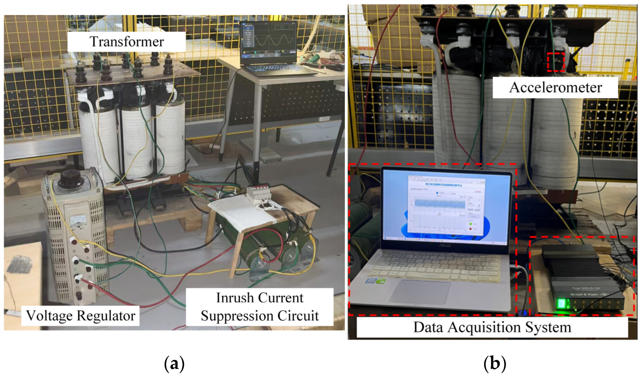
Figure 8 shows the experimental platform and vibration measurement system used for the transformer core looseness experiment. The experimental platform in Figure 8a consisted of a dry-type transformer, a three-phase voltage regulator, and an inrush current suppression circuit. The vibration measurement system in Figure 8b consisted of a B&K Type 4533-B-004 piezoelectric accelerometer and a data acquisition system comprising a B&K Type 3053-B-120 data acquisition module and a computer.

The tested transformer was a 100 kVA dry-type transformer with rated low- and high-voltage-side line voltages of 315 and 400 V, respectively. The experiment was carried out under no-load conditions. During all tests, the rated line voltage of 315 V was applied to the low-voltage side, while the high-voltage side was kept open. The supply voltage was adjusted using a TSGC2J-15 three-phase voltage regulator with a rated input of 380 V AC and an output range of 0–430 V. An inrush current suppression circuit was used to limit the no-load switching inrush current. In all tests, the sensor position and measurement direction were kept unchanged to maintain consistent measurement conditions.

A B&K Type 4533-B-004 piezoelectric accelerometer, with a nominal measurement range of ±143 g, a sensitivity of 49 mV/g, and a frequency range of 0.2 Hz–12.8 kHz, was magnetically mounted at the core lap area to measure core vibration along the lamination direction. The accelerometer signal was conditioned and digitized by the B&K Type 3053-B-120 data acquisition module and then transferred to the computer for storage.

In the experiment, core looseness was simulated by loosening the fastening bolt at the corresponding position, thereby reducing the clamping force in the core clamping region. The axial displacement of the bolt was set to 6 mm for all six looseness conditions. The six looseness positions were located at the upper and lower core-clamping regions of phases A, B, and C. These six positions defined six local core looseness conditions. Together with the normal condition, seven operating conditions were considered in this study. The category labels and their meanings are listed in

Table 1. Core looseness fault categories and label descriptions.

Category No.	Category Name	Fault Description
1	normal	Normal condition
2	Aup	Upper looseness of phase A
3	Adown	Lower looseness of phase A
4	Bup	Upper looseness of phase B
5	Bdown	Lower looseness of phase B
6	Cup	Upper looseness of phase C
7	Cdown	Lower looseness of phase C

.

4.2. Dataset Construction and Experimental Settings

For each operating condition, two groups of vibration signals were collected in separate acquisition runs under the same experimental conditions. The first acquisition was used for training and validation, whereas the second acquisition was reserved exclusively for independent testing. Each acquisition run lasted 60 s. The sampling interval was 0.0005 s, corresponding to a sampling frequency of 2 kHz. Accordingly, each acquisition run contained 120,000 sampling points for each operating condition.

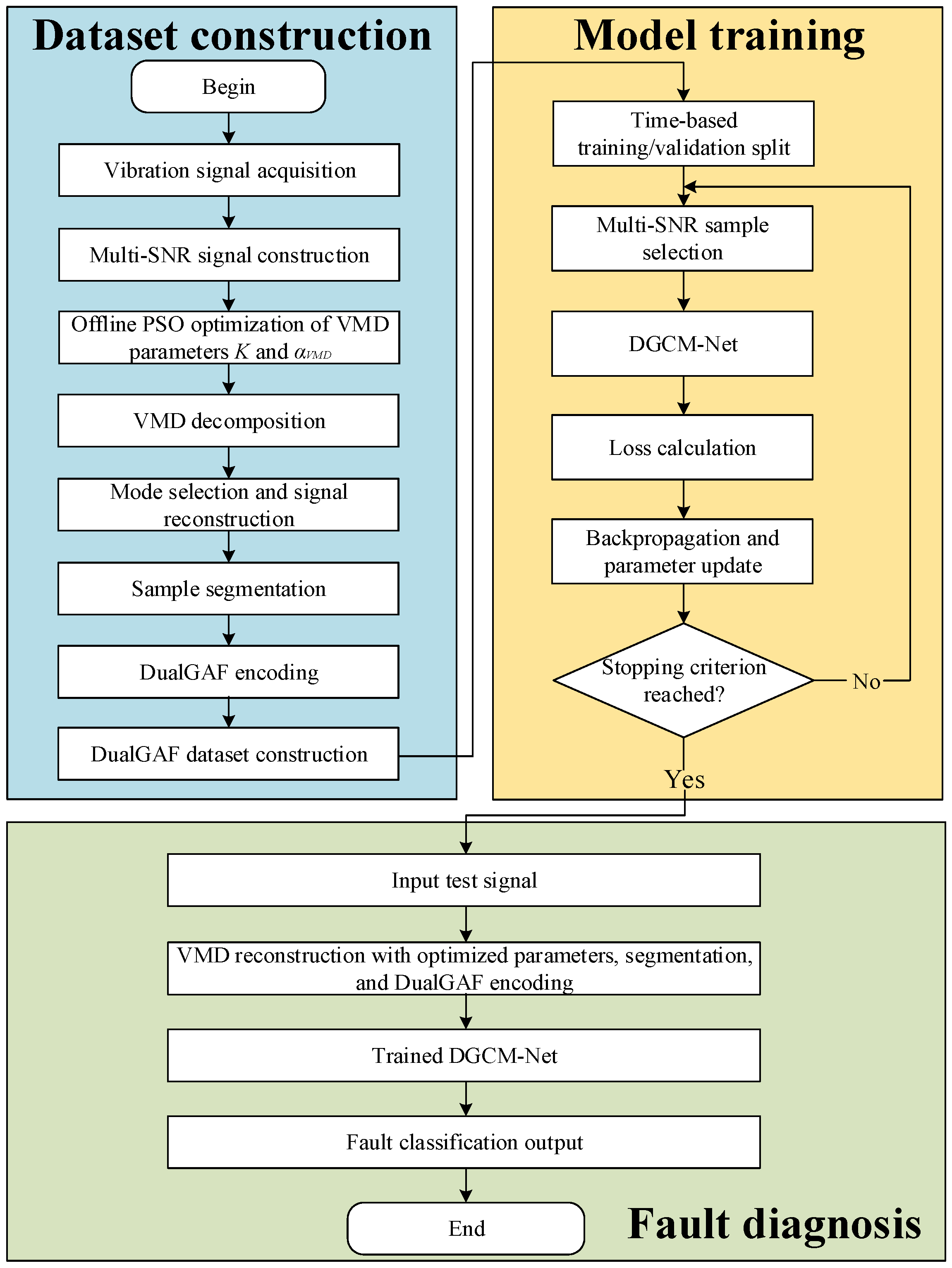
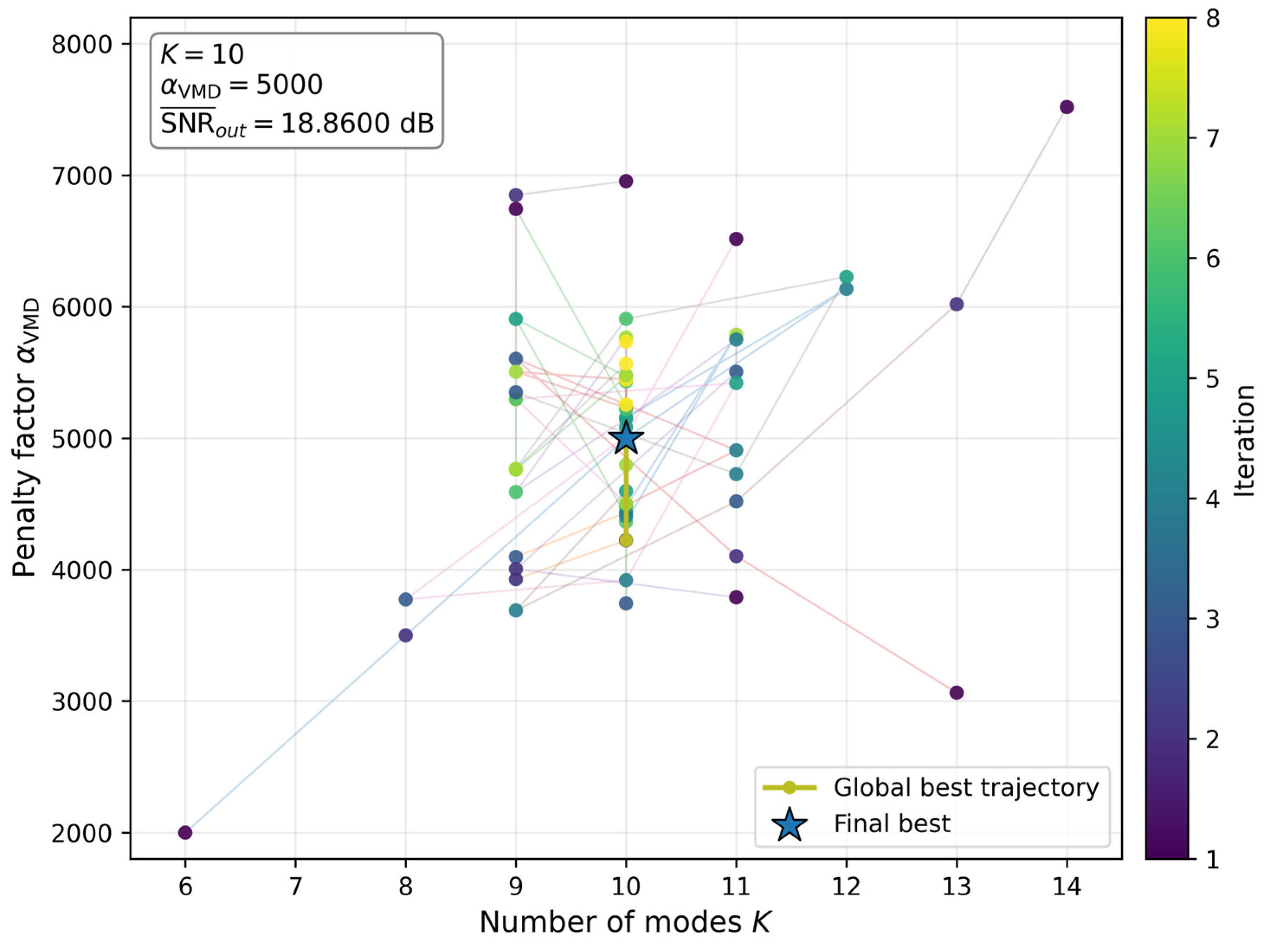
For the first acquisition, the directly measured vibration signals were treated as the standard signals. Additive white Gaussian noise (AWGN) was added to construct noisy datasets at SNRs of 25, 20, 15, and 10 dB. Before VMD reconstruction, the number of modes K and the penalty factor α_VMD were selected using particle swarm optimization (PSO). The search ranges were set to K = 6–14 and α_VMD = 2000–8000, with eight particles and eight iterations. For each operating condition, one 4000-point block was selected from the middle portion of the first acquisition, and noisy versions at the four SNR levels were generated, giving 28 evaluation samples in total. The mean output SNR after VMD reconstruction was used as the PSO objective. As shown in Figure 9, the search converged to K = 10 and α_VMD = 5000, which were used in the subsequent VMD reconstruction.

VMD reconstruction was performed using 4000-point blocks with a hop size of 2000 points. At the sampling frequency of 2 kHz, each 4000-point block corresponds to 2 s of vibration data. This duration provides enough signal points for VMD while keeping the block length at a moderate level. A 50% overlap and Hann-window weighted overlap-add were used to reduce discontinuities between adjacent reconstructed blocks.

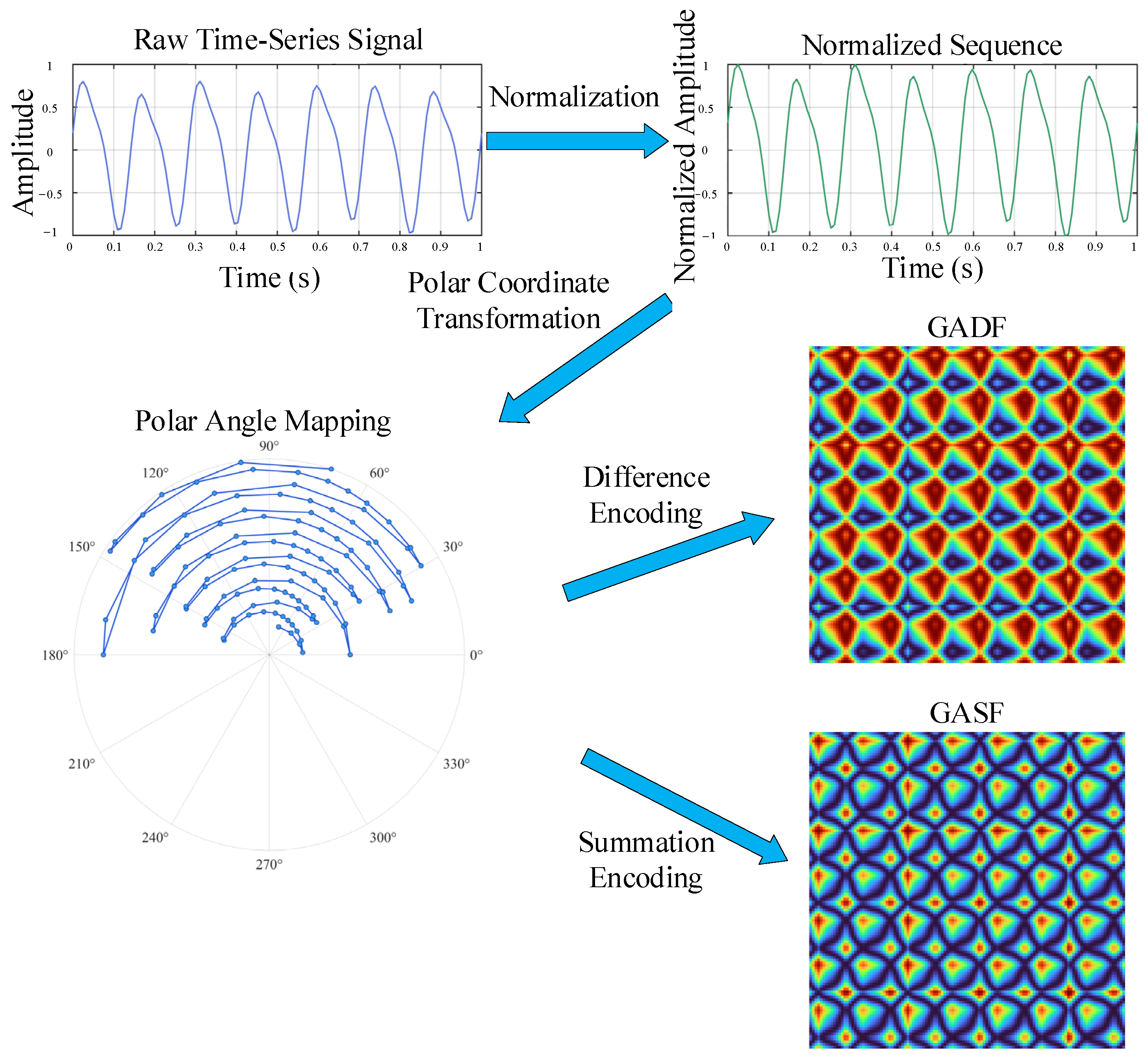
After VMD reconstruction, each signal was segmented into 600 non-overlapping windows per category, with both the window length and step size set to L = S = 200 samples. At the sampling frequency of 2 kHz, each 200-sample window corresponds to 0.1 s and contains approximately ten cycles of the dominant core-vibration component around 100 Hz. This length retains several dominant vibration cycles while providing enough temporal segments for dataset construction. For each window, the mean was removed and the signal was normalized by its standard deviation. A tanh mapping with a scaling coefficient of 0.8 was then applied before GAF encoding. This coefficient compresses large-amplitude values without strongly saturating the normalized signal.

Each signal window was encoded as 200 × 200 GASF and GADF matrices and then resized to 224 × 224 using bilinear interpolation. This resolution is close to the original GAF size and also matches the input scale commonly used with ImageNet-pretrained DenseNet121.

As shown in

Table 2. Classification performance under different input settings.

Input Setting	Standard (%)	25 dB (%)	20 dB (%)	15 dB (%)	10 dB (%)	Noisy Mean (%)
160 × 160 Gray	98.88%	98.40%	97.62%	93.79%	74.24%	91.01%
224 × 224 Gray	99.83%	99.74%	99.40%	95.81%	74.19%	92.29%
400 × 400 Gray	99.83%	99.55%	98.48%	91.45%	66.33%	88.95%
224 × 224 RGB	99.90%	99.88%	99.38%	94.45%	73.43%	91.79%

, the 224 × 224 grayscale input achieved a noisy mean accuracy of 92.29%, compared with 91.01% and 88.95% for the 160 × 160 and 400 × 400 grayscale inputs, respectively. At the same 224 × 224 resolution, the replicated red-green-blue (RGB) input gave a noisy mean accuracy of 91.79%, which was slightly lower than that of the single-channel grayscale input. Since GASF and GADF contain scalar angular-relation values, repeating the same matrix across three channels does not add new information. Therefore, 224 × 224 single-channel grayscale images were used as the network inputs.

The samples from the first acquisition were divided into training and validation subsets according to their temporal order. For each category, 400 samples were used for training and 160 samples were used for validation. A temporal gap of 20 windows on each side of the split boundary was excluded between the training and validation subsets to reduce the correlation between temporally adjacent signal segments. The same time-based split was applied to all SNR datasets so that different noise versions of the same original signal segment remained in the same subset.

During training, samples were randomly drawn from the standard-condition, 25, 20, 15, and 10 dB datasets with probabilities of 0.30, 0.05, 0.10, 0.20, and 0.35, respectively. Among the noisy conditions, the sampling probability was increased as the SNR decreased because lower-SNR signals contain stronger noise disturbances and are more difficult to classify. Standard-condition samples were kept at 30% so that clean vibration features remained sufficiently represented during training. Each epoch contained 2800 samples, with one SNR condition randomly selected for each original time window according to these probabilities. For the 10 dB validation subset, a separate AWGN realization was generated from the same first-acquisition signals. Model selection was based on the weighted validation accuracies under the standard and 10 dB conditions, with weights of 0.35 and 0.65, respectively. The larger 10 dB weight gave more importance to strong-noise performance during model selection.

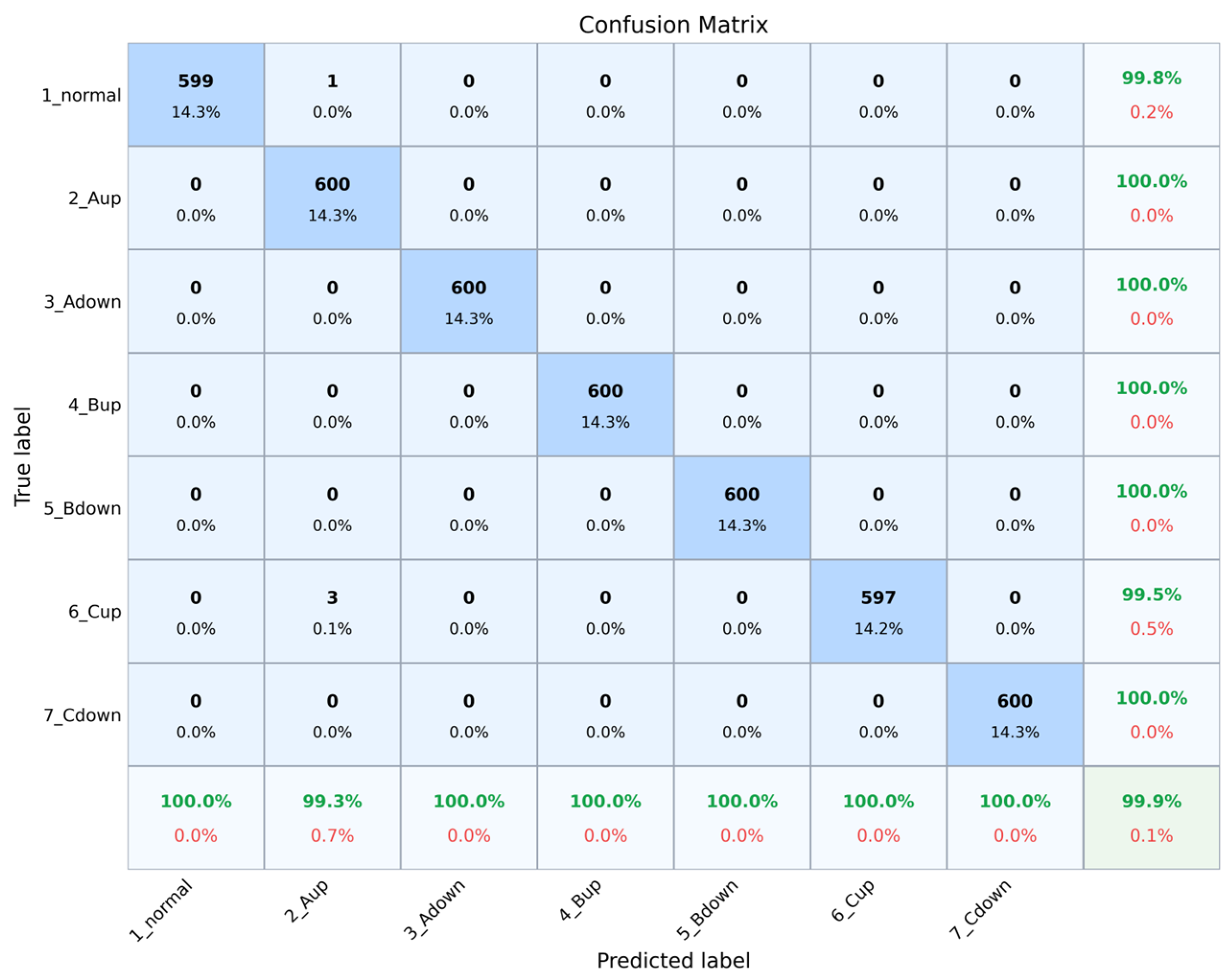
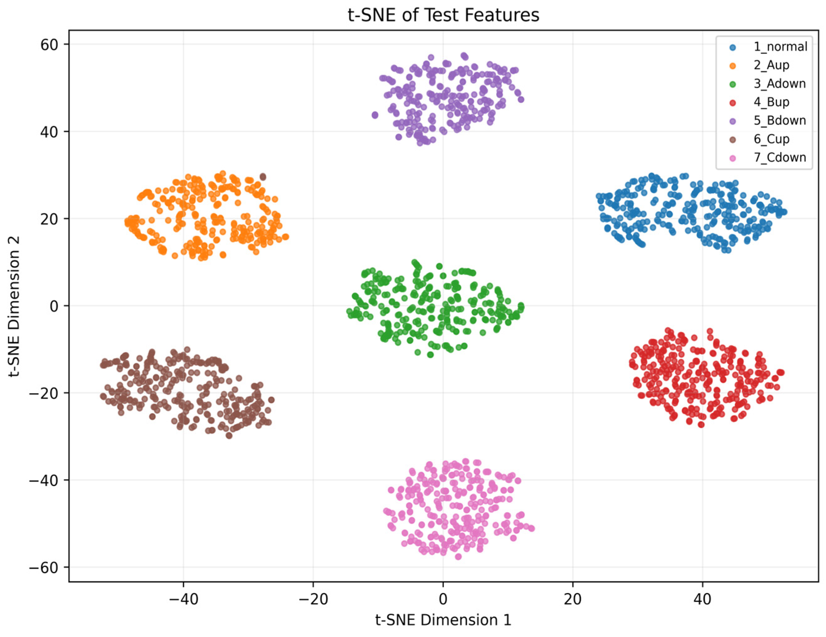
The second acquisition was reserved exclusively for independent testing and was not used for PSO parameter selection, model training, validation, or model selection. The standard test set contained 600 samples per class.

AWGN was added to the original vibration signals from the second acquisition to construct test sets at 25, 20, 15, and 10 dB. The noisy test signals were processed using the same VMD reconstruction, segmentation, normalization, and DualGAF encoding procedures as the training signals. The main VMD and training parameters are summarized in

Table 3. Main parameters used for PSO-based VMD parameter selection and signal reconstruction.

Parameter	Setting
Search range of K	6–14
Search range of αVMD	2000–8000
Number of particles	8
Number of iterations	8
Final number of modes K	10
Final penalty factor αVMD	5000
Block length	4000 points
Block hop size	2000 points
Absolute correlation threshold	0.08
Energy-ratio threshold	0.01
Spectral flatness threshold	0.80
Minimum retained modes	3
100 Hz mode-protection tolerance	±40 Hz

and

Table 4. Main training parameters of the model.

Parameter	Setting
Fused feature dimension	256
Batch size	16
Optimizer	AdamW
Loss function	Cross-entropy with label smoothing (ε = 0.03)
Training strategy	Two-stage training
Stage 1	Freeze backbones; train newly added layers
Stage 2	Unfreeze all layers for fine-tuning
Initial learning rate	Stage 1: 3 × 10−4; Stage 2: 1 × 10−4 (new layers), 2 × 10−5 (backbones)
Stage 2 learning-rate scheduler	ReduceLROnPlateau (weighted validation loss), factor = 0.5, patience = 2
Maximum epochs	Stage 1: 8; Stage 2: 40
Dropout	0.2
Weight decay	1 × 10−4
Multi-SNR sampling probabilities	Standard/25/20/15/10 dB = 0.30/0.05/0.10/0.20/0.35
Standard/10 dB validation weights	0.35/0.65

.

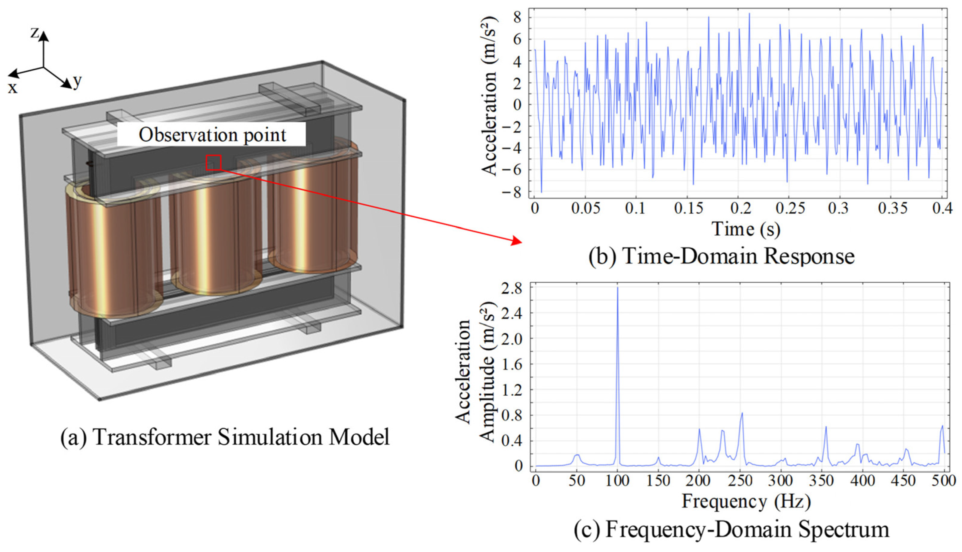
The correlation and energy-ratio thresholds were used to retain modes related to the original signal or carrying a sufficient proportion of the signal energy. The spectral-flatness threshold was used to remove modes with strong broadband noise characteristics. At least three modes were retained to avoid excessive loss of useful vibration components. The ±40 Hz range protects the mode around the dominant 100 Hz core-vibration component identified in Section 2.1. These thresholds remained fixed during PSO, while K and α_VMD were optimized.

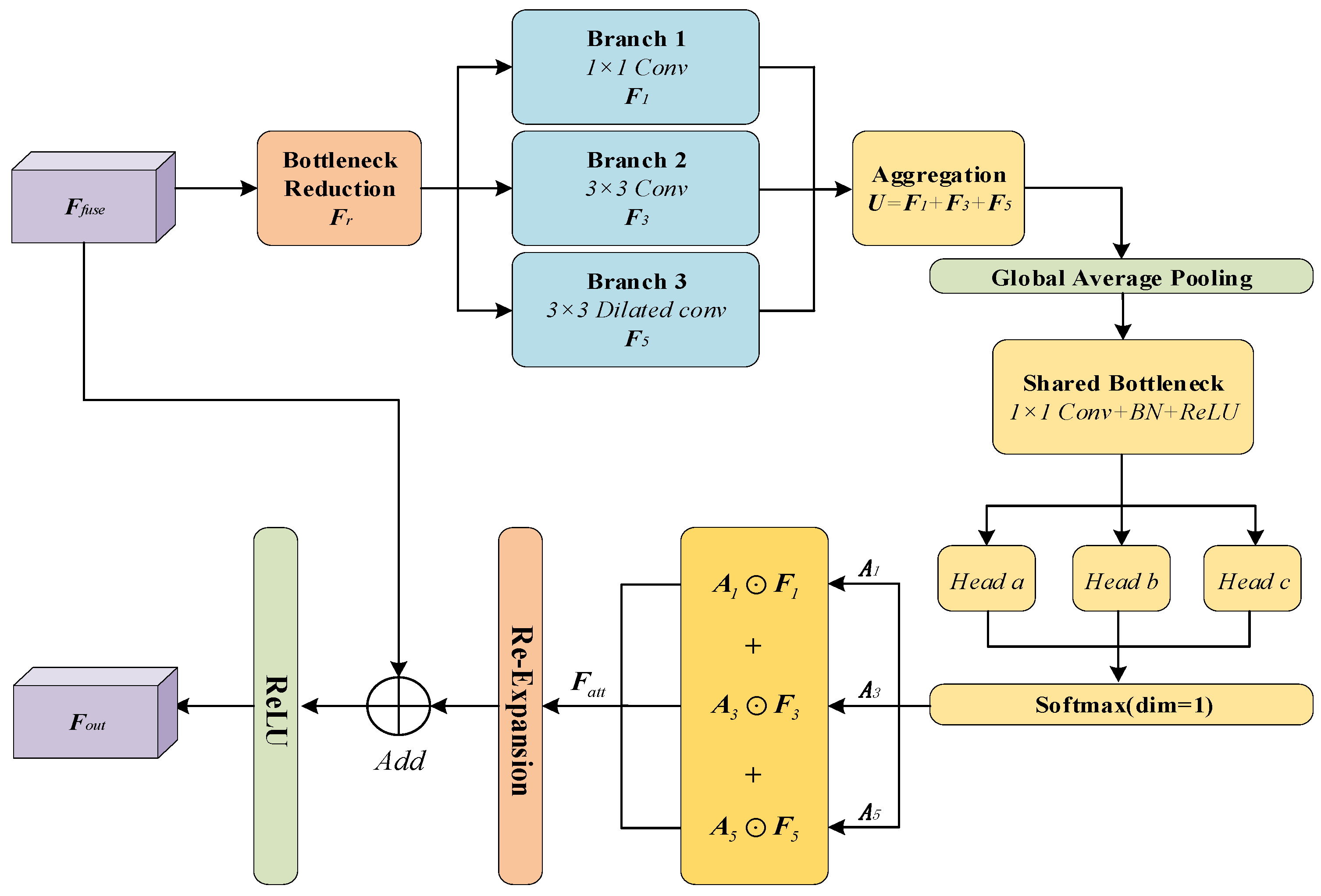
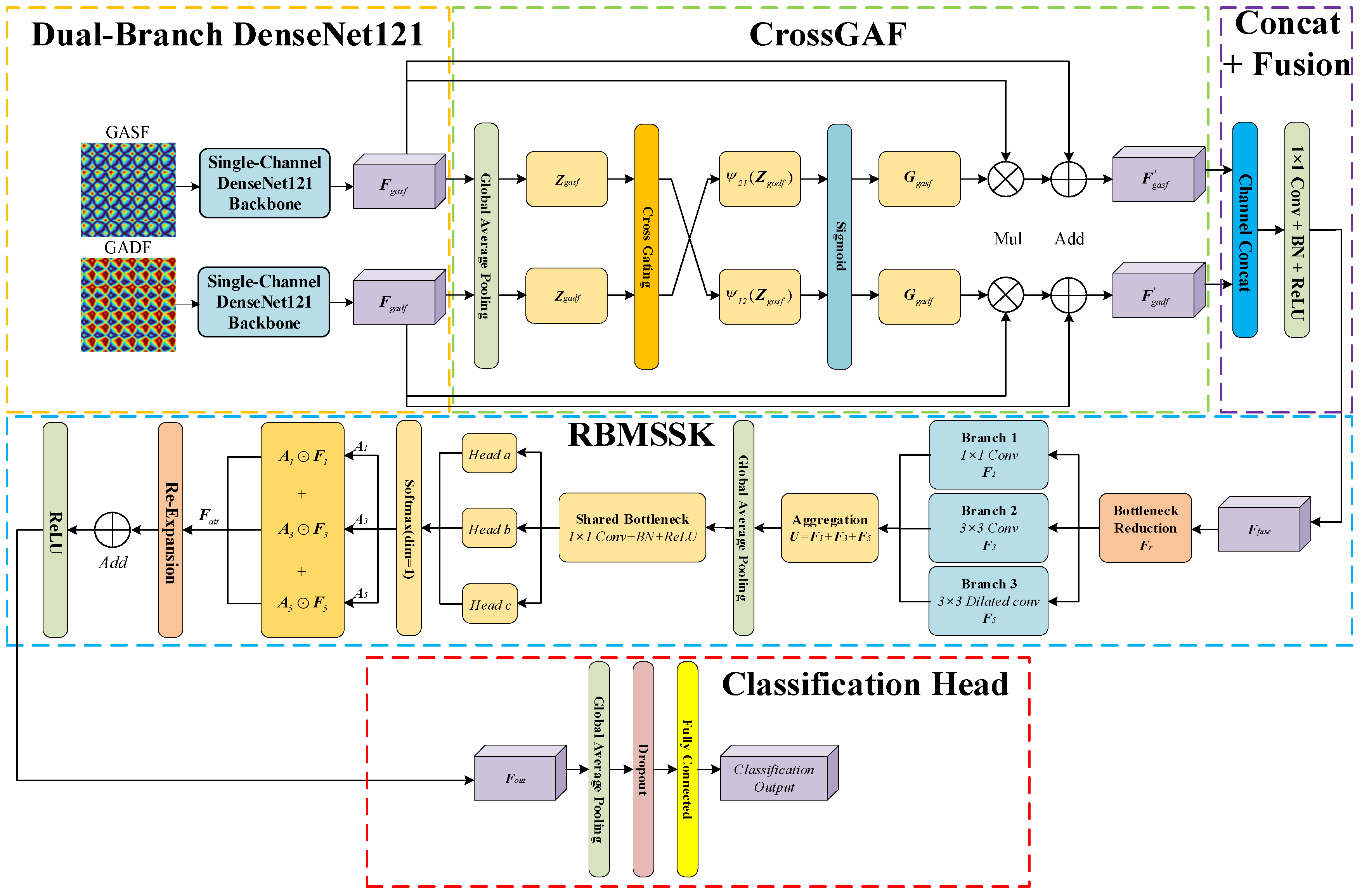
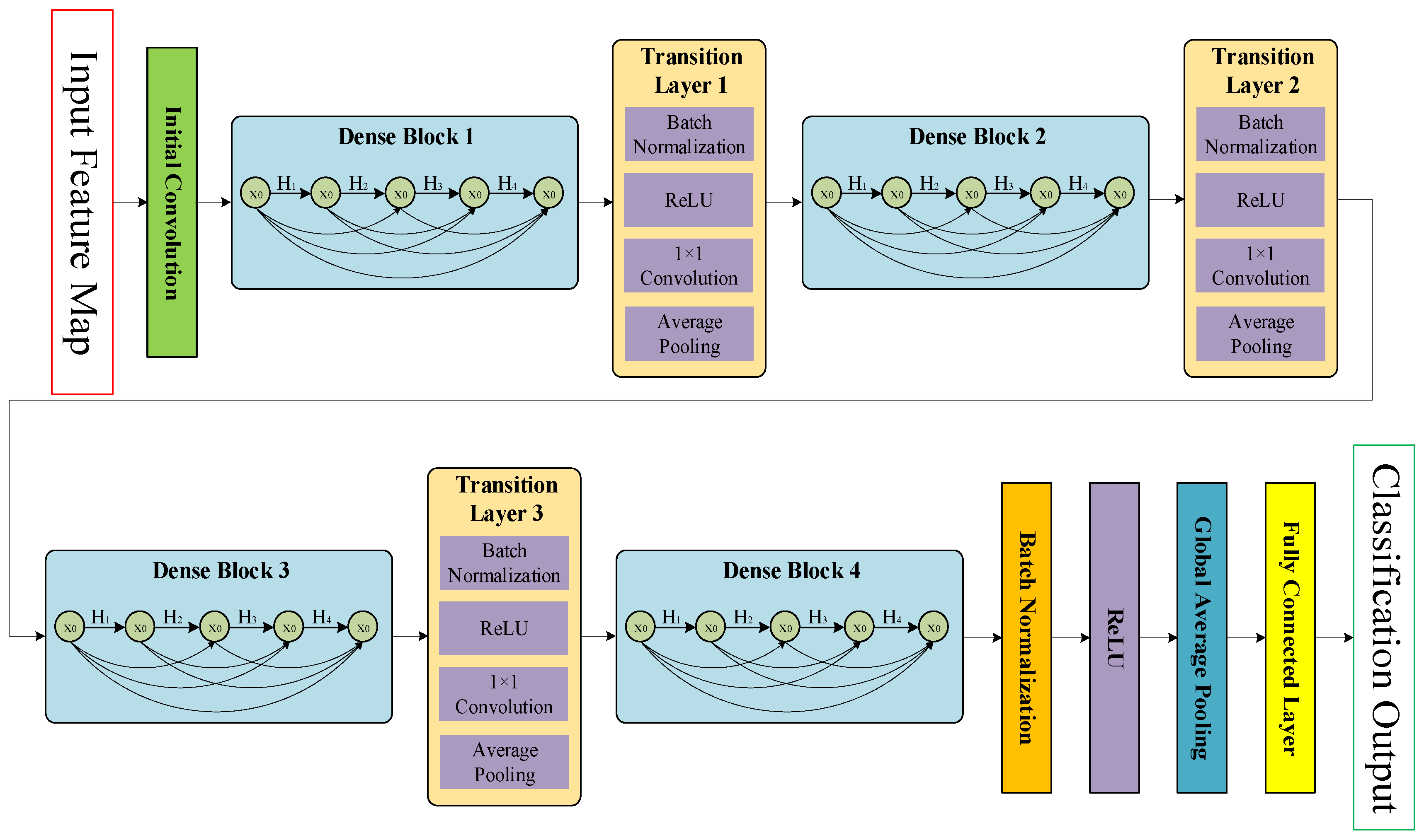
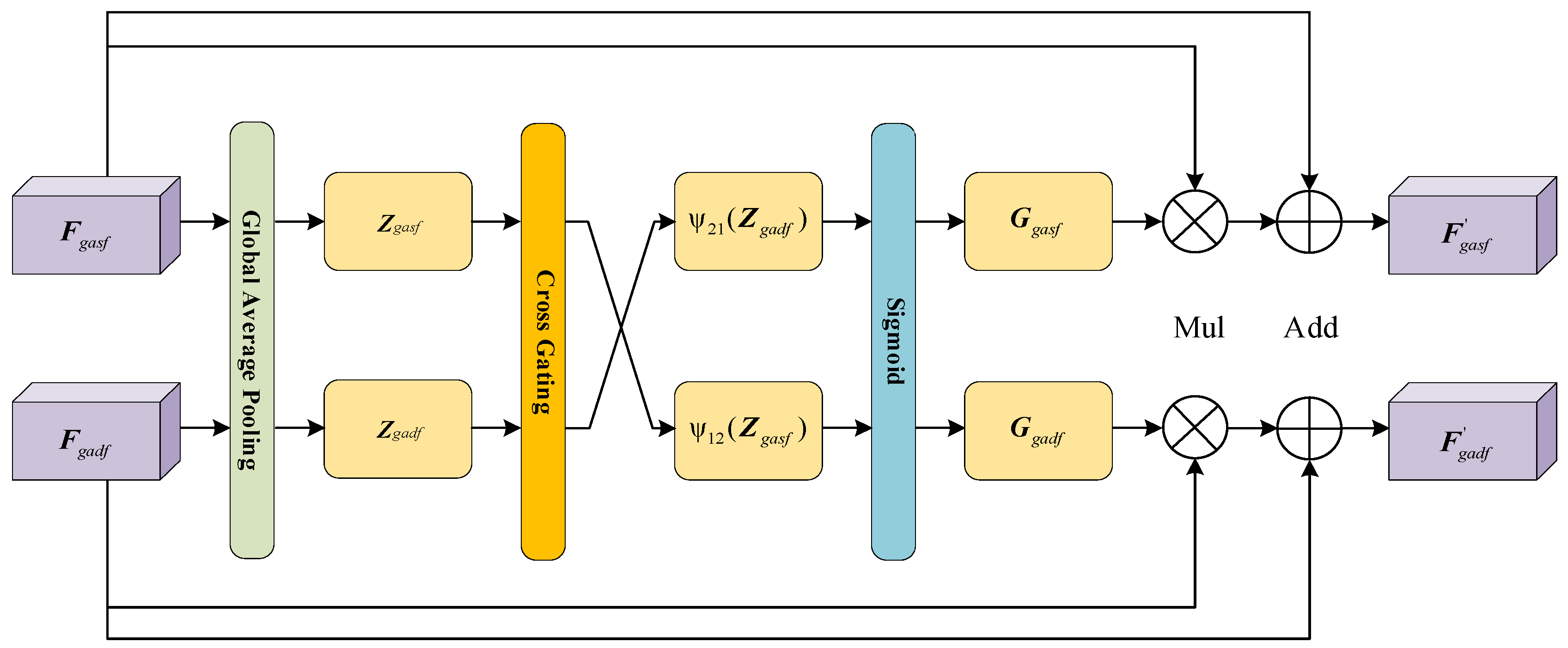
The two DenseNet121 backbones were initialized with ImageNet-pretrained weights. Since the inputs were grayscale, the first convolutional layer was changed from three channels to one, with its initial weights obtained by averaging the pretrained RGB-channel weights. Training was performed in two stages. In the first stage, the pretrained backbones were frozen so that the newly added layers could be trained first. All layers were then unfrozen for joint fine-tuning in the second stage. A lower learning rate was used for the pretrained backbones to avoid large changes to the transferred features during fine-tuning. The fused feature dimension was set to 256 to reduce the channel size after dual-branch concatenation before the RBMSSK module. A batch size of 16 was used considering the memory requirement of the dual-branch architecture. Dropout, weight decay, and label smoothing were used to reduce overfitting. The ReduceLROnPlateau scheduler reduced the learning rate when the weighted validation loss stopped improving. The main training parameters were kept consistent in the subsequent ablation and model-comparison experiments, while experiment-specific settings are described in the corresponding subsections.

Model performance was assessed using accuracy, macro precision, macro recall, and macro F1-score. From a diagnostic perspective, the normal condition was treated as the healthy state and the six looseness conditions as fault states. The missed-looseness rate, false-alarm rate, and looseness macro recall were also considered to characterize fault detection and looseness-state recognition. The missed-looseness rate is the proportion of looseness samples classified as normal, the false-alarm rate is the proportion of normal samples classified as looseness, and the looseness macro recall is the average recall over the six looseness categories. In addition, the noisy mean was calculated as the arithmetic mean of the accuracies at 25, 20, 15, and 10 dB to provide a compact summary of overall noise robustness, while the accuracy at each SNR was reported separately for condition-specific evaluation.

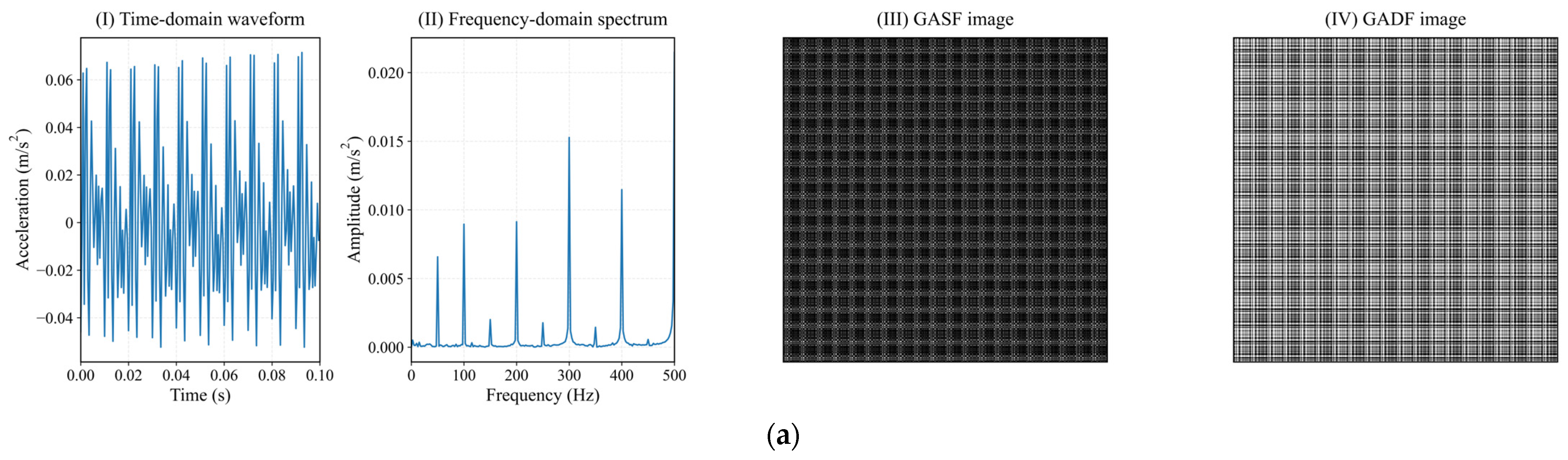
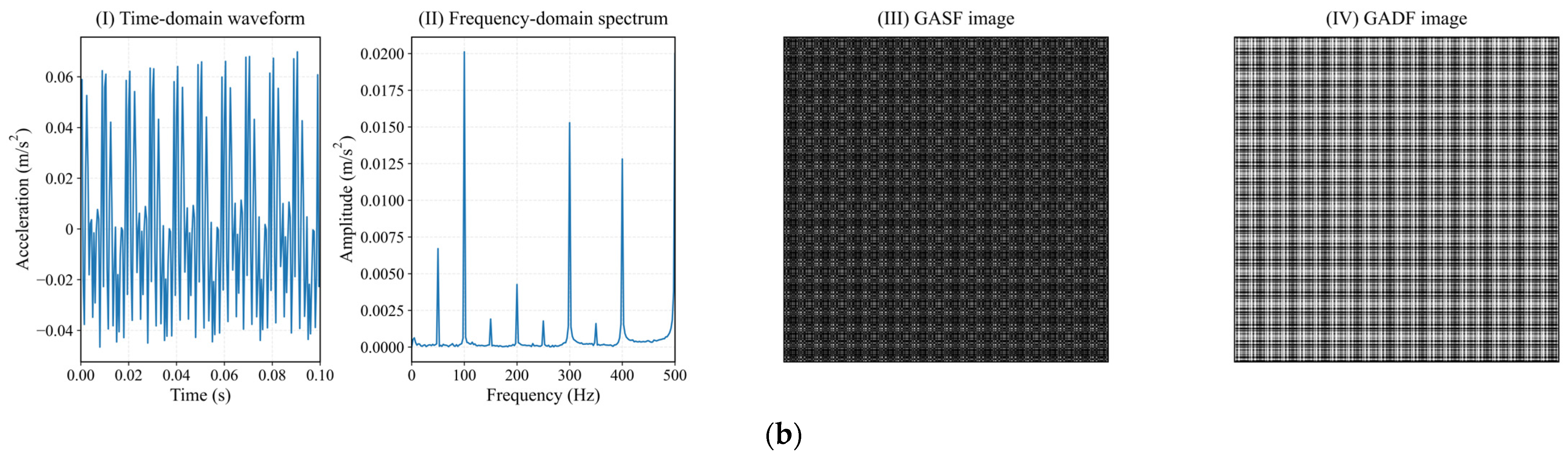
Figure 10 presents the vibration signals and corresponding GAF representations under two representative operating conditions. Figure 10a corresponds to the normal condition, whereas Figure 10b corresponds to the lower looseness condition of phase C. For visualization, a 0.1 s segment was used for the time-domain waveform, while 0.4 s and 0.2 s segments from the same starting position were used for the frequency spectrum and GAF representations, respectively.

Under the normal condition, the waveform in Figure 10a exhibits a clear periodic pattern. In the frequency spectrum, prominent components are observed around 100 Hz and its integer multiples. The corresponding GASF and GADF images exhibit structured grid-like textures and regular light–dark distributions.

Under the lower looseness condition of phase C, the waveform in Figure 10b also retains a clear periodic pattern, while differences can be observed in the local waveform shape and amplitude distribution. Compared with the normal condition, the component around 100 Hz increases markedly, while the relative amplitudes of the harmonic components also change. These changes are also reflected in the grid-like textures and local light–dark distributions of the GASF and GADF images. These differences show that condition-related variations in the vibration signals are also reflected in the GAF texture patterns.

4.3. Diagnostic Results on the Standard Test Set

To evaluate the diagnostic performance and training stability of the VMD-assisted DGCM-Net for core looseness faults, the model was independently trained five times using different random seeds and evaluated on the same independent standard test set. The mean values and standard deviations of the diagnostic metrics are listed in

Table 5. Repeated-run diagnostic results of the VMD-assisted DGCM-Net on the standard test set. SD, standard deviation.

Metric	Accuracy (%)	Macro Precision (%)	Macro Recall (%)	Macro F1-Score (%)
Mean ± SD	99.84 ± 0.11	99.85 ± 0.11	99.84 ± 0.11	99.84 ± 0.11

. The mean accuracy over the five runs was 99.84%, with a standard deviation of 0.11%. The mean macro precision, macro recall, and macro F1-score were 99.85%, 99.84%, and 99.84%, with standard deviations of 0.11%, 0.11%, and 0.11%, respectively. These results indicate that the model maintains high diagnostic performance for the seven categories, with only small variations across the five independent runs under the standard test condition.

Figure 11 presents the confusion matrix of a representative run on the independent standard test set. The test set contains 4200 samples, with 600 samples in each category. A total of four samples were misclassified in this representative run. One normal sample and three Cup samples were classified as Aup, while all samples from the other five categories were correctly identified.

Figure 12 shows the t-distributed stochastic neighbor embedding (t-SNE) visualization of the deep features from the same representative run. Samples from the same category are mainly concentrated in compact regions, and the seven categories are clearly separated in the two-dimensional embedding. This visualization indicates that the extracted deep features retain clear class-specific differences among the seven conditions under the standard test condition.

4.4. Ablation Experiment Results

4.4.1. Structural Ablation of DGCM-Net

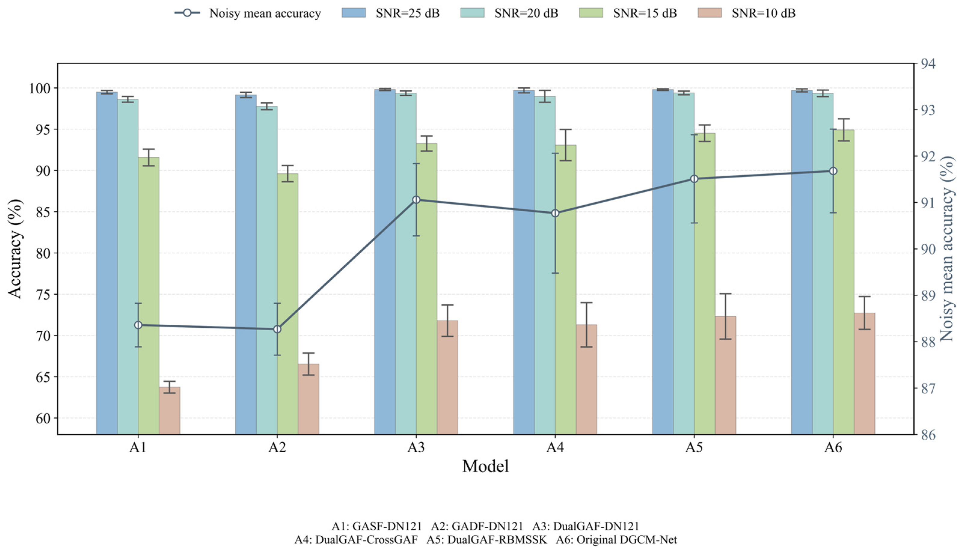
Structural ablation was performed to evaluate the effects of the DualGAF input, CrossGAF, and RBMSSK on diagnostic performance. All models were trained only on standard-condition data, without VMD reconstruction or multi-SNR training. All configurations used the same dataset split, two-stage training procedure, and independent noisy test sets. Each configuration was independently trained five times using different random seeds, and the results are reported as the mean and standard deviation over the five runs. The repeated-run results are summarized in

Table 6. Repeated-run structural ablation results and parameter counts at different SNRs.

Model	Parameters (M)	25 dB (%)	20 dB (%)	15 dB (%)	10 dB (%)	Noisy Mean (%)
A1	6.955	99.50 ± 0.20	98.63 ± 0.35	91.58 ± 1.01	63.74 ± 0.71	88.36 ± 0.47
A2	6.955	99.16 ± 0.32	97.78 ± 0.41	89.62 ± 0.98	66.54 ± 1.33	88.27 ± 0.56
A3	14.422	99.81 ± 0.12	99.37 ± 0.28	93.27 ± 0.91	71.80 ± 1.90	91.06 ± 0.78
A4	14.686	99.70 ± 0.30	98.99 ± 0.72	93.08 ± 1.89	71.30 ± 2.69	90.77 ± 1.29
A5	14.542	99.80 ± 0.10	99.40 ± 0.22	94.52 ± 1.00	72.32 ± 2.75	91.51 ± 0.95
A6	14.806	99.71 ± 0.18	99.35 ± 0.39	94.92 ± 1.34	72.73 ± 1.99	91.68 ± 0.90

and Figure 13.

Six configurations were compared. A1 and A2 are single-branch DenseNet121 models using GASF and GADF, respectively. A3 uses paired GASF and GADF inputs with two independent DenseNet121 branches but excludes CrossGAF and RBMSSK. A4 adds CrossGAF before feature fusion, whereas A5 adds RBMSSK after fusion. A6 includes both CrossGAF and RBMSSK and corresponds to the original DGCM-Net trained only on standard-condition data.

The comparison among A1–A3 shows that the advantage of the DualGAF input becomes more apparent as the SNR decreases. At 25 and 20 dB, all three configurations maintain high mean accuracies, with only small differences among them. At 15 and 10 dB, A3 reaches mean accuracies of 93.27 ± 0.91% and 71.80 ± 1.90%, exceeding A1 by 1.69 and 8.06 percentage points and A2 by 3.65 and 5.26 percentage points, respectively. Using two independent DenseNet121 branches increases the parameter count from 6.955 M for the single-branch models to 14.422 M for A3. Overall, the paired GASF and GADF inputs provide a clearer performance gain under stronger noise, with a corresponding increase in model size.

When CrossGAF is added alone, A4 remains close to A3 across all four noisy conditions. CrossGAF increases the parameter count from 14.422 M to 14.686 M, while the corresponding changes in accuracy remain small. The effect of RBMSSK is more noticeable at lower SNRs. Compared with A3, A5 increases the mean accuracy by 1.25 and 0.52 percentage points at 15 and 10 dB, respectively, while the parameter count rises only from 14.422 M to 14.542 M.

A6 combines CrossGAF and RBMSSK and represents the original DGCM-Net. At 25 and 20 dB, A6 performs similarly to A3–A5. At 15 and 10 dB, it gives the highest mean accuracies of 94.92 ± 1.34% and 72.73 ± 1.99%, respectively. Relative to A3, the gains are 1.65 and 0.93 percentage points at 15 and 10 dB, respectively, while the parameter count increases by only 2.66%, from 14.422 M to 14.806 M. Its noisy mean is also the highest, at 91.68 ± 0.90%. Overall, the original DGCM-Net gives the best low-SNR performance among the ablation configurations with only a limited increase in parameter count over A3.

4.4.2. Ablation of VMD Reconstruction and Multi-SNR Training

Four configurations were compared to evaluate the individual effects of VMD reconstruction and multi-SNR training while keeping the DGCM-Net architecture unchanged. P1 used signals without VMD reconstruction and was trained only with standard-condition samples; P2 added VMD reconstruction but retained the same training setting; P3 used signals without VMD reconstruction with multi-SNR training; and P4 combined VMD reconstruction and multi-SNR training. The time-based data split, two-stage training procedure, validation criterion, and independent test protocol were kept the same across the four configurations. Each configuration was trained independently using the same set of five random seeds.

Table 7. Repeated-run ablation results of VMD reconstruction and multi-SNR training.

Configuration	Standard (%)	25 dB (%)	20 dB (%)	15 dB (%)	10 dB (%)	Noisy Mean (%)
P1	99.91 ± 0.01	99.90 ± 0.04	99.59 ± 0.15	94.64 ± 0.62	71.93 ± 1.14	91.51 ± 0.46
P2	99.92 ± 0.01	99.89 ± 0.05	99.64 ± 0.21	97.20 ± 0.50	83.26 ± 1.20	95.00 ± 0.47
P3	99.93 ± 0.00	99.92 ± 0.01	99.79 ± 0.05	97.38 ± 0.33	86.06 ± 0.53	95.79 ± 0.22
P4	99.84 ± 0.11	99.83 ± 0.07	99.72 ± 0.10	98.70 ± 0.28	91.32 ± 0.62	97.39 ± 0.23

reports the mean and standard deviation over the five runs.

All four configurations achieve mean accuracies above 99.5% under the standard, 25 dB, and 20 dB conditions, with only small differences among them. Compared with P1, P2 increases the mean accuracy by 2.56 percentage points at 15 dB and 11.33 percentage points at 10 dB. The larger gain at 10 dB indicates that the benefit of VMD reconstruction is mainly observed under stronger noise.

A similar trend is observed when P1 is compared with P3. P3 improves the mean accuracy by 2.74 percentage points at 15 dB and 14.13 percentage points at 10 dB compared with P1. The larger improvement at 10 dB suggests that multi-SNR training is more useful under severe noise disturbance.

P4 combines both strategies and gives the highest mean accuracies at 15 and 10 dB, reaching 98.70 ± 0.28% and 91.32 ± 0.62%, respectively. Compared with P2, adding multi-SNR training provides further gains of 1.50 and 8.06 percentage points at 15 and 10 dB, respectively. Compared with P3, VMD reconstruction provides additional gains of 1.32 and 5.26 percentage points at the same two SNRs. Thus, each strategy still provides an additional improvement when the other is already included, while their combination gives the best results at 15 and 10 dB.

4.5. Comparison Experiments

Three sets of comparison experiments were conducted. First, the original DGCM-Net was compared with several DualGAF models using different backbone networks. These models were trained using only the original standard-condition data, without VMD reconstruction or multi-SNR training. The VMD-assisted DGCM-Net was then compared with several representative fault diagnosis and image classification models using the same VMD reconstruction and multi-SNR training protocol. Finally, EEMD, empirical wavelet transform (EWT), and PSO-VMD were compared using the same DGCM-Net architecture to evaluate the effect of different signal denoising methods.

4.5.1. Comparison of the Original DGCM-Net with Different Backbone Models

The effects of backbone selection and the additional feature-processing modules were examined by comparing DualGAF models based on VGG16, ResNet18, DenseNet121, and ShuffleNetV2 with the original DGCM-Net under standard and noisy test conditions. All models used DualGAF inputs and were trained using only the original standard-condition data, without VMD reconstruction or multi-SNR training. The same dataset split, two-stage training procedure, and independent standard and noisy test sets were used throughout the comparison. The models differed only in the backbone architecture or the use of the additional feature-processing modules. Each configuration was independently trained five times using the same set of random seeds, and the results are reported as the mean and standard deviation of the five runs.

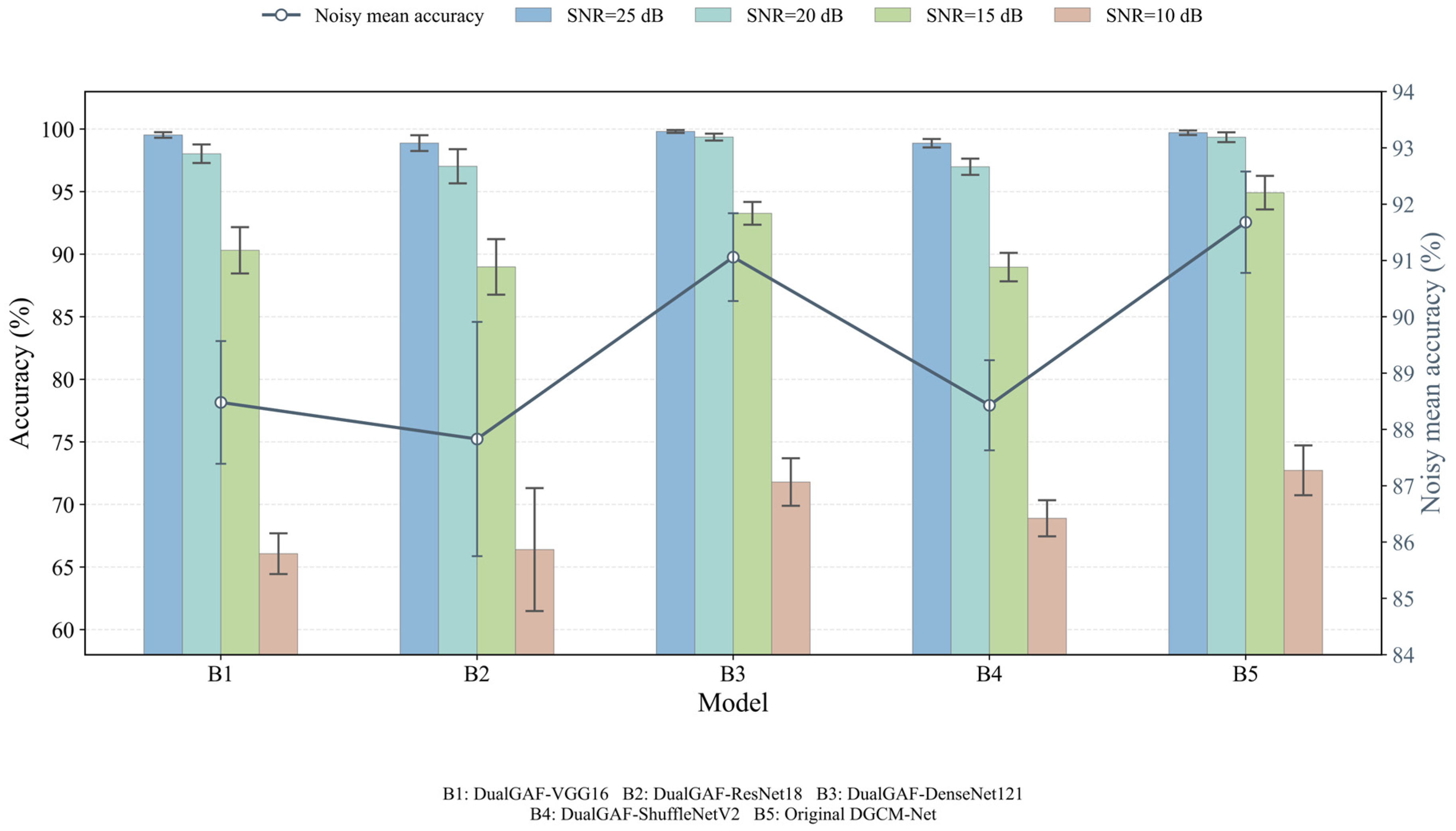
Five model configurations were compared. B1, B2, B3, and B4 denote DualGAF models using VGG16, ResNet18, DenseNet121, and ShuffleNetV2 as the backbone, respectively. B5 denotes the original DGCM-Net, which uses DenseNet121 as the backbone and further includes CrossGAF and RBMSSK. The repeated-run results are summarized in

Table 8. Repeated-run comparison results of different backbone models under standard and noisy test conditions.

Model	Standard (%)	25 dB (%)	20 dB (%)	15 dB (%)	10 dB (%)	Noisy Mean (%)
B1	99.75 ± 0.15	99.53 ± 0.22	98.03 ± 0.74	90.31 ± 1.85	66.07 ± 1.63	88.48 ± 1.09
B2	99.47 ± 0.32	98.88 ± 0.63	97.03 ± 1.37	88.99 ± 2.22	66.40 ± 4.91	87.83 ± 2.08
B3	99.89 ± 0.05	99.81 ± 0.12	99.36 ± 0.28	93.27 ± 0.91	71.80 ± 1.90	91.06 ± 0.78
B4	99.57 ± 0.19	98.87 ± 0.34	96.99 ± 0.65	88.97 ± 1.14	68.90 ± 1.44	88.43 ± 0.80
B5	99.81 ± 0.12	99.71 ± 0.18	99.35 ± 0.39	94.92 ± 1.34	72.73 ± 1.99	91.68 ± 0.90

and Figure 14.

As shown in Table 8 and Figure 14, all models maintain high mean accuracies under the standard, 25 dB, and 20 dB conditions, with relatively small performance differences. As the SNR decreases, the differences among the models become more evident. At 10 dB, B1, B2, and B4 achieve mean accuracies of 66.07 ± 1.63%, 66.40 ± 4.91%, and 68.90 ± 1.44%, respectively, showing a clear reduction compared with their performance at higher SNRs. These results indicate that the diagnostic performance of these backbone models is more affected under strong noise.

Among the four backbone models, DenseNet121 provides the best overall performance under the noisy test conditions. B3 achieves mean accuracies of 93.27 ± 0.91% and 71.80 ± 1.90% at 15 and 10 dB, respectively, and obtains the highest noisy mean accuracy of 91.06 ± 0.78% among B1–B4. Based on DenseNet121, the original DGCM-Net further introduces CrossGAF and RBMSSK. B5 achieves 94.92 ± 1.34% and 72.73 ± 1.99% at 15 and 10 dB, respectively, which are 1.65 and 0.93 percentage points higher than those of B3. Its noisy mean accuracy also increases to 91.68 ± 0.90%. These results indicate that the complete DGCM-Net provides a modest improvement over the DualGAF-DenseNet121 baseline, mainly under the lower-SNR conditions.

4.5.2. Comparison of the VMD-Assisted DGCM-Net with Representative Models

The VMD-assisted DGCM-Net was compared with MA–ResNet18 [14], dual-branch ShuffleNetV2-CBAM [18], EfficientNet-B0 [28], and MobileMamba-S6 [29] to evaluate its diagnostic performance and the trade-off between diagnostic accuracy and model complexity. The GAF-based ResNet18 architecture with multi-head attention adapted from [14] is referred to as MA–ResNet18 in this study. The parallel ShuffleNetV2 architecture with paired GASF and GADF inputs and CBAM adapted from [18] is referred to as dual-branch ShuffleNetV2-CBAM. EfficientNet-B0 was selected as an efficient convolutional model, while MobileMamba-S6 was used as a visual state-space model.

All comparison models were trained and tested using the same VMD-reconstructed datasets generated with the PSO-optimized parameters. The multi-SNR sampling strategy, time-based training and validation split with 20 windows excluded on each side of the split boundary, independent test sets, two-stage training schedule, and weighted standard and 10 dB validation criterion were kept the same. Each model was independently trained five times using the same set of random seeds, and the results are reported as the mean and standard deviation of the five runs. MA–ResNet18, EfficientNet-B0, and MobileMamba-S6 used GASF images as single inputs. In contrast, dual-branch ShuffleNetV2-CBAM and the VMD-assisted DGCM-Net used paired GASF and GADF images as inputs.

Table 9. Repeated-run diagnostic accuracy comparison of the VMD-assisted DGCM-Net with representative models.

Model	Standard (%)	25 dB (%)	20 dB (%)	15 dB (%)	10 dB (%)	Noisy Mean (%)
MA–ResNet18	98.74 ± 0.43	98.68 ± 0.39	98.17 ± 0.50	95.99 ± 0.83	85.05 ± 1.91	94.47 ± 0.82
Dual-branch ShuffleNetV2-CBAM	99.68 ± 0.05	99.51 ± 0.11	99.16 ± 0.18	96.95 ± 0.32	86.30 ± 0.52	95.48 ± 0.24
EfficientNet-B0	99.87 ± 0.02	99.80 ± 0.04	99.48 ± 0.10	97.21 ± 0.31	86.17 ± 0.92	95.67 ± 0.32
MobileMamba-S6	98.45 ± 0.32	98.18 ± 0.37	97.58 ± 0.36	94.52 ± 0.65	82.46 ± 0.97	93.18 ± 0.52
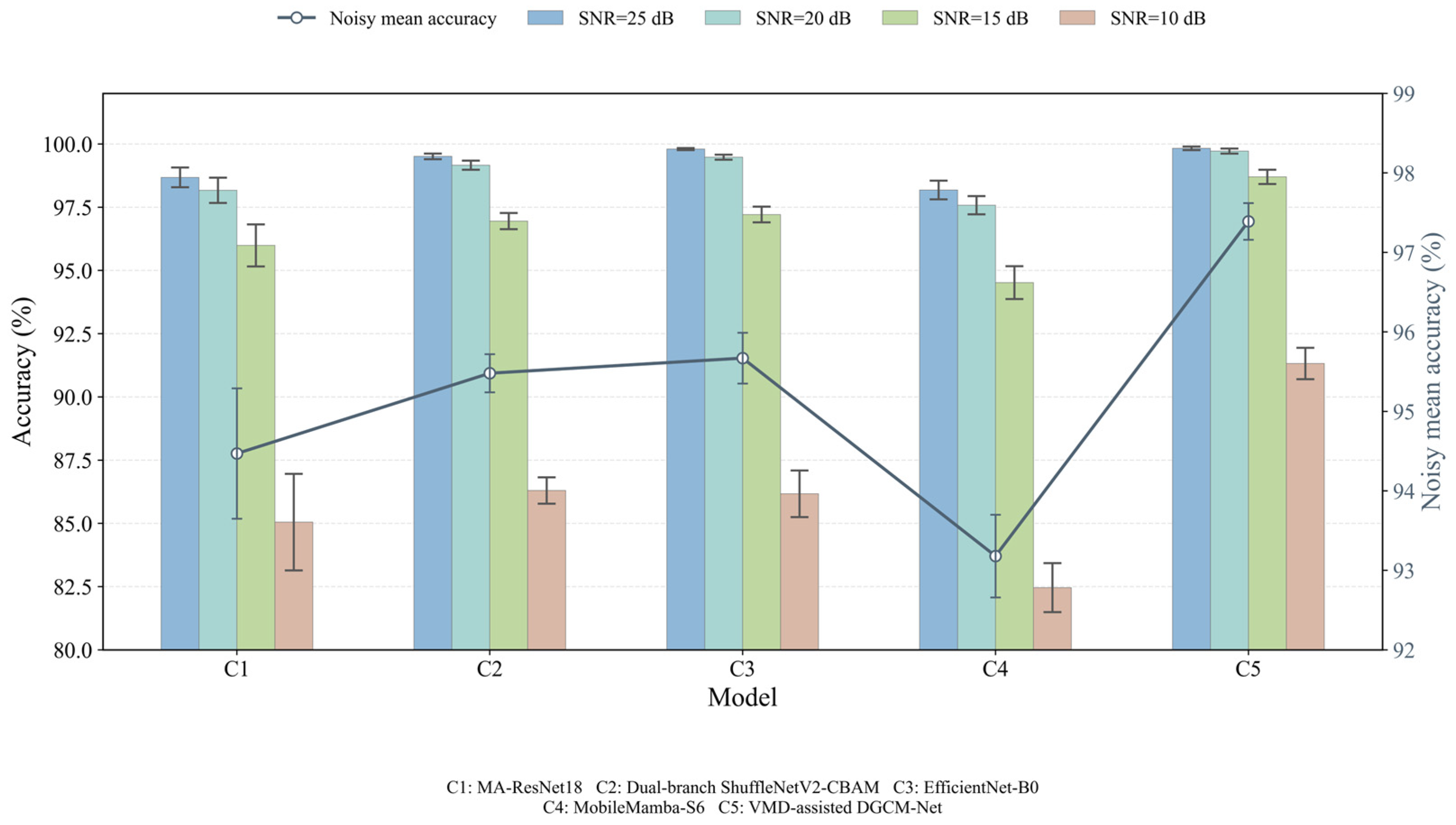
VMD-assisted DGCM-Net	99.84 ± 0.11	99.83 ± 0.07	99.72 ± 0.10	98.70 ± 0.28	91.32 ± 0.62	97.39 ± 0.23

summarizes the repeated-run comparison results, while Figure 15 shows the mean diagnostic accuracies of the five models under the four noisy test conditions.

Under the standard and high-SNR conditions, EfficientNet-B0 and the VMD-assisted DGCM-Net both achieve high diagnostic accuracies. EfficientNet-B0 obtains the highest mean accuracy under the standard condition at 99.87 ± 0.02%, while the VMD-assisted DGCM-Net reaches 99.84 ± 0.11%. At 25 and 20 dB, the VMD-assisted DGCM-Net achieves 99.83 ± 0.07% and 99.72 ± 0.10%, respectively, compared with 99.80 ± 0.04% and 99.48 ± 0.10% for EfficientNet-B0. These differences are small, indicating that the two models provide comparable diagnostic performance under the standard and high-SNR conditions.

The performance differences become clearer as the SNR decreases. At 15 dB, the VMD-assisted DGCM-Net achieves an accuracy of 98.70 ± 0.28%, which is 1.49 percentage points higher than the 97.21 ± 0.31% obtained by EfficientNet-B0. At 10 dB, the VMD-assisted DGCM-Net maintains an accuracy of 91.32 ± 0.62%. This result is 5.02, 5.15, 6.27, and 8.86 percentage points higher than those of dual-branch ShuffleNetV2-CBAM, EfficientNet-B0, MA–ResNet18, and MobileMamba-S6, respectively.

To provide a compact measure of the overall diagnostic robustness across different noise levels, the noisy mean was calculated as the arithmetic mean of the accuracies at 25, 20, 15, and 10 dB. Equal weighting was used so that the four predefined SNR conditions contributed equally to this aggregate measure, while the accuracy at each SNR was retained for condition-specific comparison. The VMD-assisted DGCM-Net obtains a noisy mean accuracy of 97.39 ± 0.23%. This value is 1.72, 1.91, 2.92, and 4.21 percentage points higher than those of EfficientNet-B0, dual-branch ShuffleNetV2-CBAM, MA–ResNet18, and MobileMamba-S6, respectively.

These results show that the advantage of the VMD-assisted DGCM-Net is mainly observed under the lower-SNR conditions. Because all comparison models used the same VMD reconstruction and multi-SNR training protocol, the remaining performance differences mainly reflect the differences in input representation and network structure. The larger performance differences at 15 and 10 dB suggest that the paired GAF representations, cross-branch interaction, and multi-scale feature processing may contribute to improved diagnostic performance when the GAF textures are strongly disturbed by noise.

The improvement under low-SNR conditions is accompanied by an increase in model complexity.

Table 10. Model complexity comparison of the VMD-assisted DGCM-Net and representative models.

Model	Parameters (M)	Inference Time (ms/Sample)
MA–ResNet18	12.225	5.13 ± 0.88
Dual-branch ShuffleNetV2-CBAM	4.084	27.80 ± 4.74
EfficientNet-B0	4.016	17.53 ± 2.59
MobileMamba-S6	14.590	41.56 ± 4.87
VMD-assisted DGCM-Net	14.806	68.54 ± 12.54

compares the parameter counts and inference times of the five models. The inference time was measured using batch-size-1 32-bit floating-point (FP32) inference on an NVIDIA GeForce RTX 4090 D after 50 warm-up iterations, followed by 200 timed forward passes. For each model, the inference time is reported as the mean and standard deviation over the five independently trained runs.

The VMD-assisted DGCM-Net contains 14.806 M parameters and has a mean inference time of 68.54 ± 12.54 ms/sample. In comparison, EfficientNet-B0 contains 4.016 M parameters and has a mean inference time of 17.53 ± 2.59 ms/sample. EfficientNet-B0 therefore has a lower computational cost while maintaining comparable diagnostic performance under the standard and high-SNR conditions. However, the accuracy difference between the VMD-assisted DGCM-Net and EfficientNet-B0 increases as the SNR decreases. The difference is 0.03 percentage points under the standard condition, but increases to 1.49 percentage points at 15 dB and 5.15 percentage points at 10 dB. These results indicate an accuracy–complexity trade-off: the proposed model has a higher computational cost, but its performance advantage becomes more evident under stronger noise.

To further examine the diagnostic performance from an application-oriented perspective, the missed-looseness rate, false-alarm rate, and looseness macro recall were compared at 10 dB. The results for the five models are summarized in

Table 11. Application-oriented diagnostic performance of the compared models at 10 dB.

Model	Missed-Looseness Rate (%)	False-Alarm Rate (%)	Looseness Macro Recall (%)
MA–ResNet18	2.22 ± 0.62	41.53 ± 3.44	89.48 ± 2.32
Dual-branch ShuffleNetV2-CBAM	1.87 ± 0.38	25.13 ± 3.37	88.20 ± 0.37
EfficientNet-B0	1.74 ± 0.54	30.57 ± 3.28	88.96 ± 1.39
MobileMamba-S6	2.29 ± 0.21	37.70 ± 2.68	85.82 ± 0.92
VMD-assisted DGCM-Net	1.39 ± 0.10	17.13 ± 0.84	92.73 ± 0.75

.

At 10 dB, the VMD-assisted DGCM-Net obtains the lowest missed-looseness rate of 1.39 ± 0.10%, corresponding to a fault detection recall of 98.61 ± 0.10%. The difference in missed-looseness rate is relatively small compared with EfficientNet-B0, which obtains 1.74 ± 0.54%. A clearer difference is observed in the false-alarm rate. The VMD-assisted DGCM-Net gives a false-alarm rate of 17.13 ± 0.84%, while the mean false-alarm rates of the other models range from 25.13% to 41.53%. The VMD-assisted DGCM-Net also obtains the highest looseness macro recall of 92.73 ± 0.75%, which is 3.25 percentage points higher than that of MA–ResNet18, the next highest model.

These results show that the performance difference at 10 dB is reflected not only in overall classification accuracy, but also in the detection and localization of core looseness. Together with the complexity comparison in Table 10, these results indicate that the higher computational cost of DGCM-Net is accompanied by improved diagnostic performance.

4.5.3. Comparison of Different Signal Denoising Methods

EEMD [7], EWT [30], and VMD [22] were compared using the same DGCM-Net to evaluate the effect of different signal denoising methods. The main parameters of all three denoising methods were determined using the training data, with parameter search used for EEMD and EWT and PSO used for VMD. The selected parameters were a noise width of 0.03, 20 trials, and a maximum of eight intrinsic mode functions (IMFs) for EEMD; six empirical wavelet components for EWT; and K = 10 and α_VMD = 5000 for VMD. The DualGAF encoding, network architecture, multi-SNR sampling strategy, time-based training and validation split, two-stage training procedure, and independent test sets were kept the same for all three methods. Each method was independently trained five times using the same random seeds. The results are reported as the mean and standard deviation of the five runs.

As shown in

Table 12. Repeated-run diagnostic accuracy comparison using different signal denoising methods.

Denoising Method	Standard (%)	25 dB (%)	20 dB (%)	15 dB (%)	10 dB (%)	Noisy Mean (%)
EEMD	92.44 ± 1.17	90.25 ± 1.20	86.10 ± 1.24	76.56 ± 1.50	63.69 ± 0.63	79.15 ± 1.07
EWT	95.66 ± 1.05	95.14 ± 1.11	94.17 ± 1.00	89.97 ± 0.87	77.09 ± 1.47	89.09 ± 1.08
PSO-VMD	99.84 ± 0.11	99.83 ± 0.07	99.72 ± 0.10	98.70 ± 0.28	91.32 ± 0.62	97.39 ± 0.23

, PSO-VMD achieves the highest mean accuracy under all five test conditions. At 15 and 10 dB, the VMD-assisted DGCM-Net achieves 98.70 ± 0.28% and 91.32 ± 0.62%, respectively, which are 8.73 and 14.23 percentage points higher than those obtained with EWT. EEMD obtains accuracies of 76.56 ± 1.50% and 63.69 ± 0.63% under the same conditions. Across the four noisy test sets, the noisy mean accuracy is 97.39 ± 0.23% for PSO-VMD, 89.09 ± 1.08% for EWT, and 79.15 ± 1.07% for EEMD.

Transformer core vibration is dominated by the component around 100 Hz and also contains several harmonic components. Core looseness changes the relative amplitudes and distribution of these components. Under additive white Gaussian noise, broadband noise may overlap with the frequency components carrying condition information. Therefore, the main periodic and harmonic components need to be retained during denoising. EEMD, EWT, and VMD decompose the signal according to different principles and therefore produce different component representations. In the VMD reconstruction, the absolute correlation coefficient, energy ratio, spectral flatness, and 100 Hz protection rule are used together for mode selection. This mode-selection procedure helps retain the main core-vibration components while suppressing part of the broadband noise. The corresponding accuracy advantage is more evident at 15 and 10 dB.

4.6. External Validation Experiments

To further examine the generalizability of the proposed framework, the public transformer vibration dataset reported by Li et al. [1] was used for additional validation. The dataset was collected from a 50 kVA dry-type transformer on a different experimental platform and contains ten operating conditions under two load levels. Two experiments were conducted using this dataset. First, the complete VMD-assisted DGCM-Net was retrained and evaluated on the 50 kVA data. Second, the representation learned from the 100 kVA data was used to initialize a few-shot adaptation model for the 50 kVA transformer.

4.6.1. External Validation Under Severe Noise Conditions

Following the 70%, 20%, and 10% split used in [1], the vibration records were divided into training, validation, and test subsets. The signals were resampled to 2 kHz before processing. The split was performed before VMD reconstruction and segmentation, and each subset was processed separately. The VMD reconstruction, signal segmentation, and DualGAF encoding procedures were the same as those used in the main experiments. For each operating condition, 280 samples were used for training, 80 for validation, and 40 for testing.

The network architecture and two-stage training procedure were unchanged. Samples from the standard, 10, 7.5, 5, and 2.5 dB conditions were sampled with equal probability during training. Model selection was based on the weighted validation accuracies under the standard and 2.5 dB conditions, with weights of 0.35 and 0.65, respectively. Five independent runs were performed with different random seeds, and the results are reported as mean ± standard deviation. The repeated-run results are summarized in

Table 13. Repeated-run diagnostic results of the VMD-assisted DGCM-Net on the public 50 kVA transformer dataset.

Condition	Accuracy (%)	Macro Precision (%)	Macro Recall (%)	Macro F1-Score (%)
Standard	99.75 ± 0.25	99.76 ± 0.24	99.75 ± 0.25	99.75 ± 0.25
10 dB	99.65 ± 0.14	99.66 ± 0.13	99.65 ± 0.14	99.65 ± 0.14
7.5 dB	99.45 ± 0.33	99.48 ± 0.31	99.45 ± 0.33	99.45 ± 0.33
5 dB	99.00 ± 0.31	99.08 ± 0.27	99.00 ± 0.31	98.99 ± 0.31
2.5 dB	98.20 ± 0.65	98.42 ± 0.51	98.20 ± 0.65	98.17 ± 0.66

.

The mean accuracy remains at or above 99.00% from 10 to 5 dB. At 2.5 dB, the mean accuracy and macro F1-score are 98.20 ± 0.65% and 98.17 ± 0.66%, respectively. The mean accuracy across the four noisy test conditions is 99.08 ± 0.30%. The standard deviation of accuracy does not exceed 0.65 percentage points across the tested conditions.

The public dataset differs from the main experimental dataset in transformer capacity, experimental platform, load condition, and fault configuration. These results extend the evaluation of the proposed framework to a different transformer system and experimental setting.

4.6.2. Cross-Transformer Few-Shot Adaptation

A cross-transformer few-shot adaptation experiment was conducted using the 100 kVA transformer as the source domain and the public 50 kVA transformer as the target domain. Samples from both load levels were included and grouped into the normal and core-looseness classes. Fourteen samples were selected from each of the four original conditions, giving 56 target-domain training samples in total. The final VMD-assisted DGCM-Net trained on the 100 kVA data with the multi-SNR strategy was used as the source model. All network parameters except the final classification layer were transferred to initialize the target model, and the binary classifier was reinitialized for the target task.

Only 5% of the available target-domain training samples were used for adaptation, and all target-domain samples used for adaptation and validation were clean samples without added noise. The train/validation/test partition used in Section 4.6.1 was retained, and the test subset was used only for final evaluation. For the target-only model, the DenseNet121 backbones were initialized with ImageNet-pretrained weights, while no parameters from the 100 kVA source model were used. The same target data and training settings were used for both models. Both settings were repeated with five random seeds and evaluated under the standard, 10, 7.5, 5, and 2.5 dB conditions.

Table 14. Repeated-run results of cross-transformer few-shot adaptation on the public 50 kVA transformer dataset.

Condition	Transfer Accuracy (%)	Target-Only Accuracy (%)	Transfer Macro F1-Score (%)	Target-Only Macro F1-Score (%)
Standard	99.75 ± 0.56	97.13 ± 3.94	99.75 ± 0.56	97.11 ± 3.96
10 dB	99.50 ± 0.81	95.13 ± 6.71	99.50 ± 0.82	95.09 ± 6.76
7.5 dB	98.88 ± 2.18	94.00 ± 8.40	98.87 ± 2.19	93.97 ± 8.44
5 dB	97.13 ± 3.11	93.00 ± 9.63	97.12 ± 3.13	92.94 ± 9.71
2.5 dB	93.13 ± 4.72	92.38 ± 9.38	93.05 ± 4.82	92.30 ± 9.47

summarizes the repeated-run accuracy and macro F1-score of the transferred and target-only models under the standard and four noisy test conditions.

The transferred model achieves higher mean accuracy than the target-only model under all tested conditions. Across the four noisy conditions, the average accuracy increases from 93.63% to 97.16%, with the largest gain of 4.88 percentage points at 7.5 dB. The transferred model also has a lower standard deviation at each noisy test condition.

With only limited labeled target data, the representation learned from the 100 kVA transformer provides a more effective initialization than target-only training. The consistent improvement across the tested conditions supports the transferability of the learned representation between the two transformer systems.

5. Conclusions

This paper develops a VMD-assisted DGCM-Net with multi-SNR training for transformer core looseness diagnosis. The VMD mode number and penalty factor are optimized by PSO, and selected modes are used to reconstruct the measured vibration signals before paired GASF and GADF encoding. Two independent DenseNet121 branches extract features from the two representations. CrossGAF introduces information exchange before fusion, while RBMSSK processes the fused features at multiple scales.

Across five independent runs, the proposed method achieves 99.84 ± 0.11% accuracy under the standard condition and 97.39 ± 0.23% mean accuracy across the 25, 20, 15, and 10 dB test sets, including 91.32 ± 0.62% at 10 dB. Compared with the configuration without VMD reconstruction and multi-SNR training, the noisy mean accuracy increases by 5.88 percentage points, and the accuracy at 10 dB increases by 19.39 percentage points. The performance difference from lighter models is small under the standard and high-SNR conditions, but becomes clearer as the SNR decreases. At 10 dB, the proposed model gives a missed-looseness rate of 1.39 ± 0.10%, a false-alarm rate of 17.13 ± 0.84%, and a looseness macro recall of 92.73 ± 0.75%. On the public 50 kVA transformer dataset, the retrained model achieves 98.20 ± 0.65% accuracy at 2.5 dB. In the cross-transformer few-shot experiment, using 5% of the target-domain training samples increases the mean accuracy across the four noisy conditions from 93.63% to 97.16% compared with target-only training.

The main experiments were conducted on a single 100 kVA dry-type transformer under no-load conditions, with a fixed 6 mm bolt displacement used to simulate core looseness. Validation on the public 50 kVA transformer dataset further supports the applicability of the framework to a different transformer system and the transferability of the learned representation under limited labeled target data. Future work will extend the evaluation to more transformer types, looseness severities, operating conditions, and field noise, while reducing the computational cost for online monitoring.