A Lightweight Small-UAV Detection via Synergistically Enhanced YOLOv11

Abstract

Detecting small unauthorized UAVs against complex backgrounds is challenging: targets can be just a few pixels wide, background clutter is pervasive, and the detection system must run on resource-constrained edge hardware. This paper presents a lightweight detector built on YOLOv11 that jointly addresses background suppression and edge-deployment efficiency. A serial channel-spatial attention module is embedded into the backbone to sharpen target features and suppress interference. DySample preserves edge details during resolution recovery, and the detection head is restructured by adding a high-resolution P2 branch while removing the large-object P5 head, shifting the focus to small targets without inflating the model. The WIoU v3 loss function stabilizes training by automatically down-weighting low-quality samples. On the DUT Anti-UAV dataset, the proposed model obtains 92.2% mAP@0.5 and 61.5% mAP@0.5:0.95 with only 2.11 M parameters, a reduction of 18.2% relative to the YOLOv11n baseline. Its ability to generalize across different scenarios is verified by cross-dataset evaluation on Det-Fly and LRDDv2. Deployed on an NVIDIA Jetson Orin Nano Super with TensorRT FP16 optimization, the system achieves 37 end-to-end FPS. These findings demonstrate that the presented method significantly improves small-target detection in complex backgrounds while maintaining a lightweight design suitable for real-time edge deployment.

1. Introduction

UAVs are now routinely used in logistics, environmental monitoring, and emergency response [1]. Unregulated UAV flights, however, pose a growing threat to public safety and privacy. In sensitive areas such as airports, government sites, and large public venues, an unauthorized drone can cause serious safety incidents or be exploited for illegal surveillance [2]. Accurate, efficient detection of unauthorized UAVs is therefore an urgent technical need in low-altitude security.

Current anti-UAV systems rely heavily on radar, radio frequency analysis, acoustic sensing, and infrared spectroscopy [3]. These technologies perform well in dedicated security deployments, but they are expensive, complex to set up, and difficult to fuse across multiple sensing modalities. For large-scale civilian use, they do not easily provide wide-area, flexible, and low-cost coverage. Vision-based detection offers a compelling alternative. Cameras are inexpensive, easy to deploy, and capture rich spatial and appearance information. With the rapid development of deep learning-driven object detection, both two-stage methods such as Faster R-CNN [4] and one-stage methods such as SSD [5] have substantially improved detection accuracy. In real-time UAV detection tasks, however, their inference speed often falls short of industrial frame-rate requirements. The YOLO series, owing to its favorable accuracy–speed trade-off compared with both traditional two-stage detectors and computationally intensive Transformer-based architectures, has become the mainstream framework for real-time vision-based detection, particularly for resource-constrained edge deployment.

Yet applying YOLO models directly to low-altitude UAV detection still confronts three challenges. First, UAV targets can be extremely small. At longer distances, a drone may span only a few pixels. Features are sparse, and conventional detectors respond weakly. Second, backgrounds are diverse and unpredictable. A drone may appear against the sky, buildings, trees, or farmland, and its color and texture often blend into the surroundings. This confuses the detector, leading to false positives and missed detections. Third, practical security systems run on embedded or edge devices with tight computational budgets. Any improvement in detection accuracy must be achieved under a strict lightweight constraint.

Researchers have proposed several YOLO variants to address these challenges. Cheng et al. [6] developed IRWT-YOLO, which integrates image segmentation for background suppression, enlarges the receptive field through a DCPPA module, and captures long-range dependencies via an RCSCAA module. While effective, the deep integration of segmentation and detection increases the computational load, which becomes problematic on resource-constrained edge platforms. Yu et al. [7] designed ESOD-YOLOv8, using second-order central difference to suppress background interference and multiple auxiliary modules to boost small-target performance. The module stacking, however, raises model complexity. Ding et al. [8] proposed DCR-YOLO, which combines dynamic upsampling with attention mechanisms in a coordinated design. Its accuracy–efficiency balance is promising, but the model still leaves room for further lightweighting. A common thread runs through these works: they improve detection, but at a parameter or computational cost that can be hard to justify on edge hardware. What is missing is a method that strengthens small-target discrimination systematically, with near-zero additional overhead.

Based on the YOLOv11 framework, this paper proposes a lightweight anti-UAV detection method tailored for complex backgrounds and edge deployment. First, a lightweight attention mechanism is embedded into the backbone network, where it sharpens the features of small targets and diminishes background interference. Second, dynamic upsampling is adopted to preserve fine edge details during resolution recovery. Third, the detection head is restructured to concentrate on small-scale targets while controlling model size. Fourth, a robust loss function is applied to stabilize bounding box regression under noisy training conditions. The main contributions are as follows.

(a)

Architecture-level improvements for small-target feature retention.

A lightweight Serial channel-spatial attention (SCSA) module is embedded into the backbone, strengthening target responses and suppressing background clutter with negligible parameter cost. The detection head is restructured by adding a high-resolution P2 head and removing the large-object P5 head, shifting detection focus to small targets while reducing model size. Dynamic upsampling (DySample) replaces fixed interpolation, preserving edge details during resolution recovery without extra computation.

(b)

A training strategy robust to low-quality samples.

The Wise-IoU (WIoU) v3 loss function serves to regularize bounding box regression and prevent training instability. Its dynamic non-monotonic focusing mechanism automatically down-weights samples with imprecise boundaries—such as motion-blurred or occluded drones—preventing noisy annotations from destabilizing training. This proves essential when multiple feature-modifying modules are combined.

(c)

Systematic validation on public datasets and an edge platform.

The method is evaluated on DUT Anti-UAV and cross-dataset evaluation on Det-Fly and LRDDv2. Deployment on a Jetson Orin Nano Super with TensorRT FP16 optimization achieves real-time inference (37 FPS) with a 7.9 MB engine and 155 MB peak memory.

2. Related Work

Anti-UAV detection methods fall into two broad categories: those based on physical signals and those based on vision. Physical-signal-based methods—radar, radio frequency, acoustic, and infrared—each have their strengths, but they share a common limitation for civilian deployment: bulky equipment, high cost, and complex setup. Vision-based detection offers a lower-cost, easier-to-deploy alternative, which has made it the focus of recent anti-UAV research.

The rapid progress of vision-based detection has been driven by deep learning object detection frameworks. Faster R-CNN and other two-stage detectors rely on region proposal plus fine-grained classification to deliver high accuracy, yet their inference speed is difficult to reconcile with real-time requirements. One-stage detectors, represented by SSD and the YOLO series [9], skip the proposal stage and gain significant efficiency. The YOLO family in particular has steadily pushed the accuracy–speed frontier, evolving through the Cross Stage Partial Network (CSPNet) and Path Aggregation Network (PANet) structures in YOLOv4 [10], the engineering refinements in YOLOv5 [11], the RepBlocks in YOLOv6 [12], the E-ELAN in YOLOv7 [13], anchor-free detection in YOLOv8 [14], and the Cross Stage Partial with kernel size 2 (C3k2) and Spatial Pyramid Pooling Fast (SPPF) modules in YOLOv11 [15]. When applied directly to anti-UAV detection, however, general-purpose YOLO models still struggle: the target occupies only a tiny fraction of the image, the background is complex and unpredictable, and the resulting feature confusion leads to unacceptable false positives and missed detections.

To address small-object detection, several strategies have been proposed. Bo et al. [16] introduced InceptionNeXt and an improved SPPFCSPC-SR structure into YOLOv7 to preserve fine details. Jiang et al. [17] designed DRBD-YOLOv8, combining RCELAN attention with a weighted bidirectional feature pyramid for feature enhancement at reduced complexity. Nie et al. [18] developed DSOD-YOLO, which uses a dual-backbone architecture to strengthen detail capture, followed by pruning and knowledge distillation. These methods improve small-target performance, but their response remains weak under extreme scales—when the target spans only a few dozen pixels—and some of the added structures are not lightweight-deployment friendly.

In the face of complex background interference, researchers have explored both feature enhancement and attention mechanisms. Hong et al. [19] proposed AAD-YOLO, which integrates Sobel edge detection with dynamic upsampling to suppress background interference by sharpening spatial and edge information. Aghili et al. [20] designed YOLO-PICO with an expanded attention module for spatial-channel feature fusion, achieving accurate small-target recognition in remote sensing imagery at very low computational overhead. On the attention side, the Convolutional Block Attention Module (CBAM) [21] guides the network from both channel and spatial dimensions; the Squeeze-and-Excitation (SE) module [22] recalibrates channel responses via global pooling; and coordinate attention further injects positional information into channel weights to preserve spatial structure. Most existing attention modules, however, were not designed with an explicit parameter budget in mind. Achieving strong channel-spatial discrimination without inflating the model calls for a more disciplined structural design.

Improvements in loss functions have also contributed to small-object detection. Traditional IoU loss experiences gradient vanishing in cases where the predicted box and its corresponding ground-truth box fail to intersect. The sequence of Generalized-IoU (GIoU), Distance-IoU (DIoU), and Complete-IoU (CIoU) addresses this by adding geometric constraints: minimum enclosing rectangle, center-point distance, and aspect ratio. Zhang et al. [23] proposed Shape-IoU, which focuses on the shape and scale of the bounding box itself for more accurate regression. In the WIoU series, a dynamic non-monotonic focusing mechanism is introduced to assign differentiated gradient gains to samples of different quality levels. This mechanism is particularly relevant when the training set contains low-quality samples with imprecise boundaries, a common case in UAV detection with motion blur and occlusion.

Feature fusion and upsampling strategies have likewise been refined for small objects. Feature Pyramid Network (FPN) [24] propagates semantic information top-down, and PANet [25] adds a bottom-up path to strengthen localization signals. The lightweight Cross-Scale Feature Fusion Module (CCFM) [26] unifies channel counts before fusion, reducing computational cost while preserving feature consistency. In the upsampling step, standard bilinear interpolation is content-agnostic. Content-Aware ReAssembly of FEatures (CARAFE) [27] generates content-aware sampling kernels but incurs substantial computational overhead. DySample [28] reformulates upsampling from a point-sampling perspective, producing sampling offsets through simple linear layers. Its parameter footprint and inference speed approach those of bilinear interpolation, making it a practical choice for lightweight deployment.

The use of Transformer-based architectures has recently emerged in vision-based anti-UAV applications. Yu et al. [29] proposed a unified Transformer tracker, Wang et al. [30] designed a Swin Transformer-based tracking network for UAV swarms, and Li et al. [31] built an efficient ViT tracking framework. The self-attention mechanism excels at long-range dependencies, offering advantages in complex scene understanding. However, these models typically require large-scale training data and significant computational resources. Their performance drops when training data is limited, and their model size conflicts with the constraints of resource-constrained edge platforms. For similar reasons, two-stage detectors such as Faster R-CNN, while offering high accuracy, incur substantial inference latency that precludes real-time deployment on edge hardware. These considerations collectively motivate our choice of the YOLO framework as the foundation for lightweight anti-UAV detection.

In summary, existing methods have steadily improved anti-UAV detection, but achieving high accuracy on extremely small targets in complex backgrounds, under a strict lightweight constraint, remains an open problem. The method proposed in this paper targets this gap through coordinated improvements to feature enhancement, upsampling, detection head structure, and loss design.

3. Methods

3.1. Overview of YOLOv11

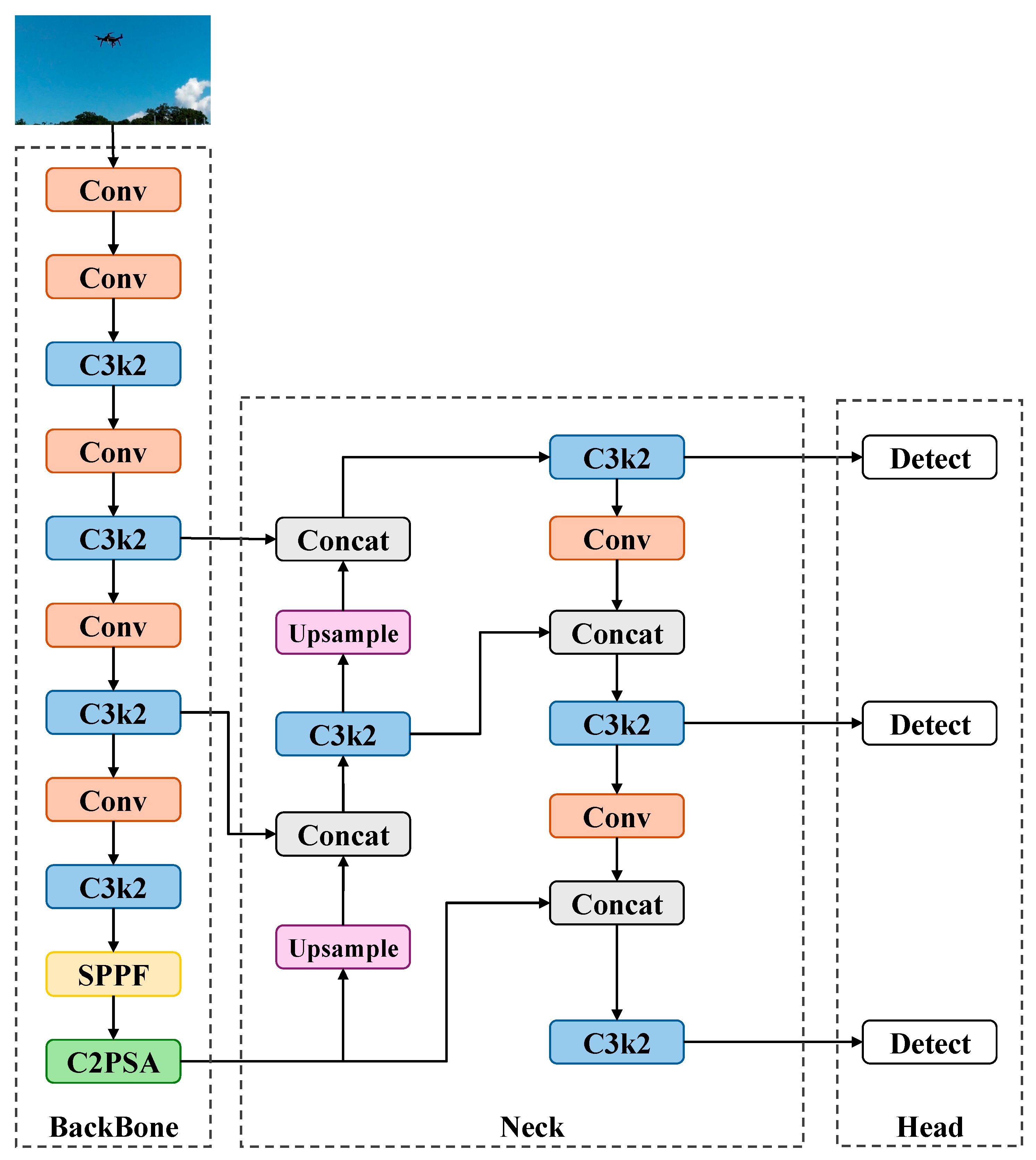
YOLOv11 inherits the standard Backbone–Neck–Head design while introducing several improvements over earlier versions. In the backbone, the C3k2 module takes the place of C2f to enable more efficient extraction of features, and the SPPF module is kept to provide multi-scale contextual information. Additionally, a Cross Stage Partial with Spatial Attention (C2PSA) module is added to enhance the network’s response to salient regions. The neck employs a PANet architecture for bidirectional multi-scale feature aggregation, while the head uses an anchor-free decoupled structure that separates the tasks of classification and regression. Figure 1 illustrates the overall architecture.

On generic detection tasks, YOLOv11 performs well. When applied to low-altitude UAV detection, however, two limitations become apparent. First, after multiple downsampling stages, the features of extremely small UAV targets are heavily attenuated, and the shallow detail information does not reach the detection layers effectively. Second, the standard feature extraction path provides no explicit mechanism for suppressing complex background interference. These two issues motivate the improvements introduced in the following sections.

3.2. The Improved Overall Framework

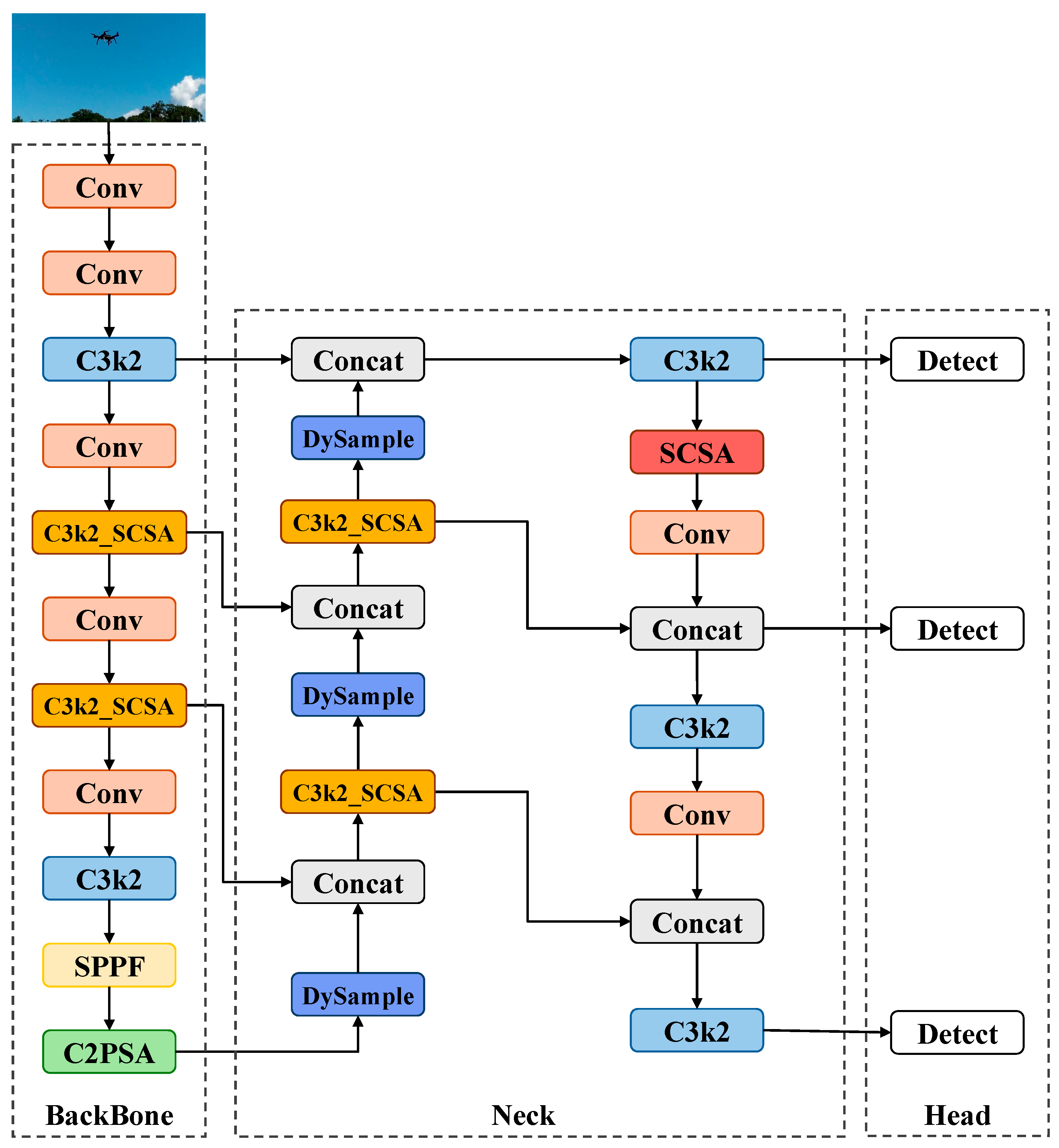
In low-altitude anti-UAV detection, YOLOv11 faces a tough combination: targets are often just a handful of pixels, yet the background can vary sharply from open sky to cluttered terrain, depending on the scene. Under these conditions, fine-grained features of extremely small drones tend to wash out in deep layers, and the network struggles to ignore the kind of background interference that changes scene by scene. This paper tackles both problems through coordinated changes to the backbone, neck, head, and loss function. The overall architecture is shown in Figure 2.

In the backbone, we replace the standard C3k2 module with C3k2_SCSA. This module embeds a lightweight serial channel-spatial attention that adds almost no parameters or FLOPs. It works by first suppressing non-drone regions spatially, and then recalibrating channel responses to amplify the features that matter for small targets—essentially giving the backbone an early focus on what is likely a drone and what is clearly not.

In the neck, the usual fixed interpolation is replaced by DySample dynamic upsampling. Standard upsampling tends to smooth over fine edges, which hurts when a target is only a few pixels wide. DySample adapts to local content and preserves those edge details better during resolution recovery. In parallel, we integrate C3k2_SCSA into the feature fusion paths and place an extra SCSA block before the P2 layer input, further reinforcing the high-resolution representations that are critical for spotting very small drones.

For the head, we observed that drone targets in these scenes rarely occupy more than a tiny fraction of the frame. That makes the P5 detection head—designed for large objects—mostly idle. We therefore remove it and add a dedicated P2-based small-object head instead. The shift concentrates the detection capacity on small scales without inflating the model size.

For training, the standard IoU loss is replaced with WIoU v3. Its outlier-aware dynamic focusing automatically down-weights samples whose bounding box labels are likely imprecise, a common problem for extremely tiny or motion-blurred drones. This keeps low-quality annotations from destabilizing regression, which matters a lot when the background is complex and the aircraft is moving.

Section 3.3, Section 3.4, Section 3.5 and Section 3.6 detail the design and implementation of each module.

3.3. Design of Serial Channel-Spatial Attention (SCSA) Module

The original C3k2 module in YOLOv11 extracts features using standard convolutional stacks and residual connections, treating all channels and spatial positions equally without any dedicated selection mechanism. In low-altitude anti-UAV detection, the drone occupies an extremely small pixel area, making its feature response prone to being swamped by intricate backgrounds. At the same time, the C3k2 module has no explicit way to suppress background interference, which distracts the model’s attention and results in false positives and missed detections. Such limitations call for a lightweight attention mechanism embedded directly into the feature extraction stage, aiming to enhance discrimination of small targets while reducing background influence.

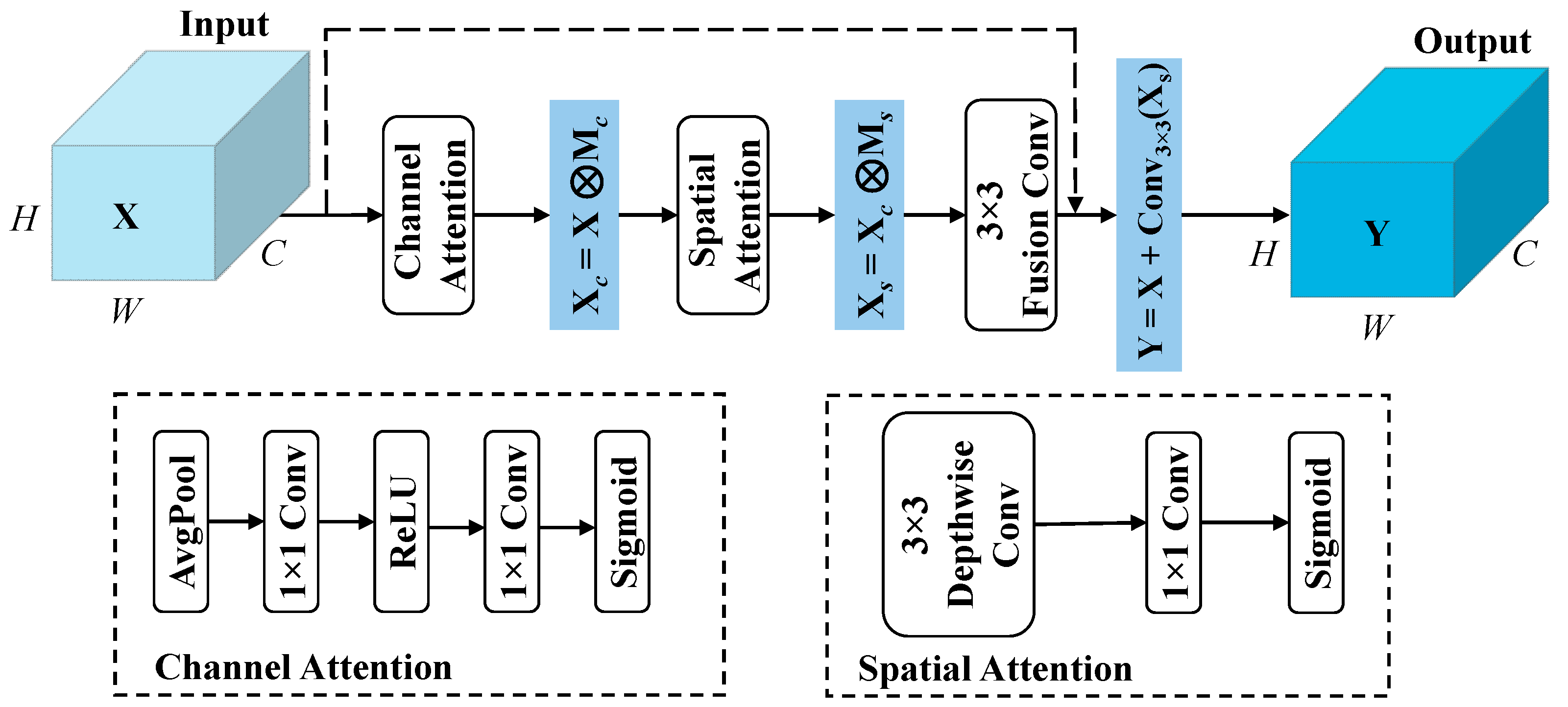
To address the above issue, this paper integrates the SCSA into the C3k2 module, resulting in the C3k2_SCSA module, whose overall structure is illustrated in Figure 3. This module adopts a “channel-first, spatial-second” serial attention architecture: the channel attention first performs global average pooling and a 1 × 1 convolution to recalibrate per-channel importance. This guides the model to prioritize channels that contain information most useful for distinguishing small targets. Then, spatial attention is applied to the enhanced features and employs a 3 × 3 depthwise convolution to capture spatial structure—a choice that keeps the spatial branch almost parameter-free while still identifying where the target is and where the background dominates. The two stages are cascaded in series to complement each other by first screening the critical channels, then locating the key positions. This gives the feature extractor a clear ‘select and focus’ behavior, at almost no extra parameter cost.

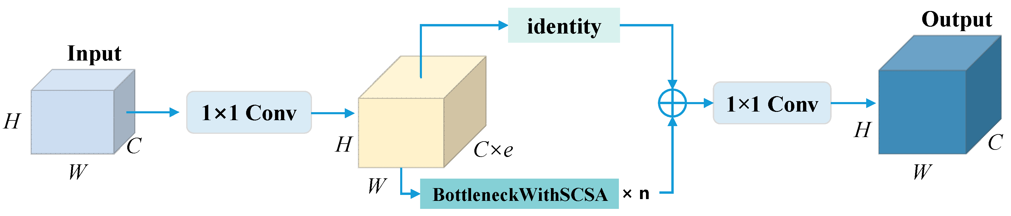
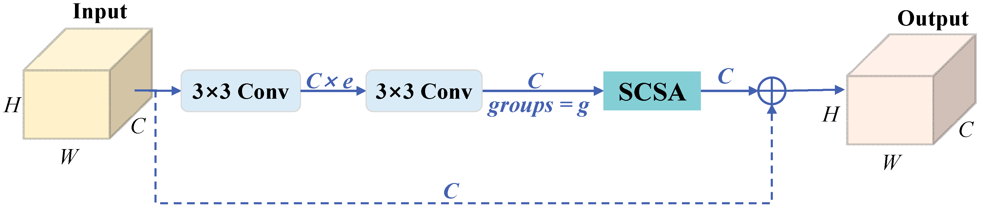
The C3k2_SCSA module is built upon the original C3k2 backbone, where several Bottleneck units are replaced by SCSA-equipped BottleneckWithSCSA units. Figure 4 depicts the internal structure of a BottleneckWithSCSA unit. Inside this unit, the input features initially pass through a standard convolution for channel transformation, after which grouped convolution extracts spatial features. These resulting features are then delivered into the SCSA module, where channel attention and spatial attention are sequentially applied. Following a refinement step via a fusion convolution, the features are ultimately combined with the original input through a residual connection, yielding the enhanced output features.

Figure 5 illustrates the structure of the SCSA module. Starting from an input feature map $\mathit{X}\in {\mathit{R}}^{C\times H\times W}$, the channel attention branch initially performs adaptive average pooling on X, reducing the spatial dimensions to 1 × 1 and producing a channel descriptor vector. This vector subsequently goes through two 1 × 1 convolutions, ReLU, and a Sigmoid activation in sequence, yielding the channel attention weights ${\mathit{M}}_{\mathbf{c}}\in {\mathit{R}}^{C\times 1\times 1}$. The input features are then multiplied channel-wise by these weights, giving the channel-enhanced features ${\mathit{X}}_{\mathbf{c}}=\mathit{X}\odot {\mathit{M}}_{\mathbf{c}}$. The spatial attention branch takes ${\mathit{X}}_{\mathbf{c}}$ as input, employs a 3 × 3 depthwise convolution to extract spatial structural information, and then compresses the channel dimension to 1 via a 1 × 1 convolution, followed by Sigmoid activation to produce the spatial attention weights ${\mathit{M}}_{\mathbf{s}}\in {\mathit{R}}^{1\times H\times w}$. The element-wise multiplication of ${\mathit{X}}_{\mathbf{c}}$ and the spatial weights yields the spatially enhanced features ${\mathit{X}}_{\mathbf{s}}={\mathit{X}}_{\mathbf{c}}\odot {\mathit{M}}_{\mathbf{s}}$. After being refined by a 3 × 3 convolution, ${\mathit{X}}_{\mathbf{s}}$ is added to the original input X via a residual connection to obtain the following final output:

Y = X + Conv_3×3 (X_s)

(1)

The residual connection ensures smooth gradient propagation while allowing the network to retain original feature information even when attention enhancement is not needed.

It is worth contrasting our SCSA with the widely adopted CBAM, as both share a similar high-level principle of serial channel-first, spatial-second attention. However, our SCSA differs from CBAM in three substantial aspects. First, CBAM applies channel compression through a reduction ratio, which inevitably loses fine-grained channel information. For extremely small UAV targets where feature signals are inherently weak, such compression may discard the very cues needed for discrimination. Our SCSA, in contrast, preserves the full channel capacity throughout the attention process without any reduction. Second, CBAM employs standard convolutions in its spatial branch, introducing non-negligible parameter overhead. Our SCSA instead utilizes a 3 × 3 depthwise convolution, maintaining nearly zero additional parameters while effectively capturing spatial structure. Third, beyond structural differences, our SCSA incorporates a residual connection that fuses the attention-refined features with the original input, enabling stable gradient propagation and preserving original feature information. These design choices render SCSA substantially more parameter-efficient than CBAM while providing superior feature refinement capability for small-target detection under strict resource constraints.

Through the above joint channel-spatial enhancement mechanism, the SCSA module autonomously focuses on important channels and target regions during feature extraction, continuously strengthens small-target features and suppresses background interference throughout the multi-scale fusion process, thereby producing more discriminative feature representations in complex scenarios.

3.4. DySample Dynamic Upsampling Module

The Neck of YOLOv11 by default adopts nearest-neighbor interpolation for upsampling, with a fixed sampling grid that treats all positions in the feature map equally. In low-altitude anti-UAV detection scenarios, fixed upsampling lacks content-awareness, and the sampling points cannot distinguish between target regions and background noise: the edge and texture details of small targets are smoothed during upsampling, while background noise is proportionally amplified as the resolution increases. Together, these two effects degrade the quality of features passed to the fusion stage, making it harder to separate small drones from their surroundings.

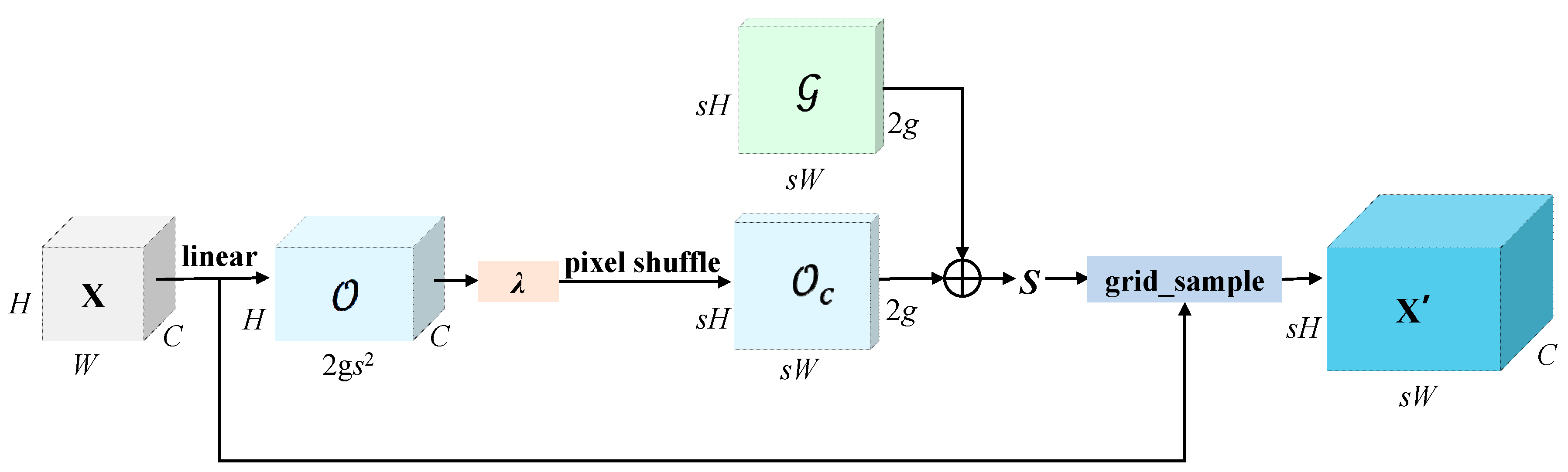
To address this issue, this paper introduces the DySample dynamic upsampling module. DySample redefines the upsampling process from the perspective of point sampling, learning content-aware sampling offsets so that the sampling points can adaptively adjust their positions according to feature response intensity. In practice, the sampling points are drawn toward strong gradient responses during training. Because even a few-pixel drone produces noticeable gradients at its boundaries, the points tend to lock onto target contours rather than diffusing into the background. In flat background regions, the sampling points remain uniformly distributed, avoiding additional noise amplification. Compared with dynamic upsampling methods that require generating full upsampling kernels, DySample predicts only a small number of sampling offsets through linear layers, resulting in extremely low parameter and computational overhead, with inference speed close to that of bilinear interpolation, which renders it well-suited for deployment on edge hardware with limited resources.

Figure 6 presents the architecture of DySample. Starting from an input feature map $\mathit{X}\in {\mathit{R}}^{C\times H\times W}$ and an upsampling factor s, the module initially produces a content-aware offset $\mathcal{O}$ using a linear layer (implemented as a 1 × 1 convolution). The channel count of this offset is 2 × G × s², where G denotes the number of groups, and these 2 × G × s² channels encode the displacements along the x and y axes for each upsampled point.

$$\mathcal{O}=\mathrm{l}\mathrm{i}\mathrm{n}\mathrm{e}\mathrm{a}\mathrm{r}\left(\mathit{X}\right)$$

(2)

Next, the static range factor λ scales the offset $\mathcal{O}$, thereby limiting how far the sampling points can shift, preventing excessive misalignment caused by overly large offsets. The initial sampling grid $\mathcal{G}$ is initialized with bilinear interpolation, whose zero-offset state is equivalent to the output of standard bilinear interpolation. The constrained offset ${\mathcal{O}}_{\mathrm{c}}$ is added to the initial grid to obtain the final sampling coordinates S:

$$\mathit{S}=\mathcal{G}+{\mathcal{O}}_{\mathrm{c}}$$

(3)

To reduce the number of parameters, DySample adopts an LP (Linear + Pixel Shuffle) structure. It first generates low-resolution offset information through a linear layer, and then applies pixel shuffling to obtain sampling coordinates that match the resolution after upsampling. Finally, the input feature map is resampled in continuous space using the grid_sample function to obtain the upsampled feature map ${\mathit{X}}^{\prime }\in {\mathit{R}}^{C\times sH\times sW}$:

$${\mathit{X}}^{\prime }=\mathrm{grid}\_\mathrm{sample}(\mathit{X},\mathit{S})$$

(4)

Through the above content-aware dynamic sampling strategy, DySample guides the sampling points to shift toward the interior of the target boundaries in object edge regions, preserving clear edges; in background regions, it maintains uniform sampling and suppresses noise amplification. This gives the upsampled features cleaner object boundaries, and that extra sharpness helps the detection head separate drones from complex backgrounds later on.

3.5. P2 Small-Object Detection Head and Structural Optimization

The original detection head of YOLOv11 corresponds to three feature layers: P3, P4, and P5, among which P5 has the lowest resolution and is primarily designed for large object detection. In low-altitude anti-UAV scenarios, target sizes are generally extremely small, and the coarse-grained features handled by the P5 layer contain almost no valid information about small targets, while its corresponding convolutional layers and prediction branches introduce parameter redundancy. Meanwhile, the P2 feature map, with its high resolution, retains rich edge and texture details, offering a natural advantage for small-target localization; however, the original design does not connect it to the detection head. To address these two issues, this paper restructures the detection head: a high-resolution small-object detection head based on the P2 feature layer is added, and the large-scale P5 detection head is removed, resulting in a three-level detection head architecture comprising P2, P3, and P4. With the P2 head, shallow fine-grained features can directly inform detection, which sharpens localization of extremely small targets. Dropping P5 removes convolutions and prediction branches that are idle in our setting, keeping the model compact without any downside.

To further enhance the discriminative capability of the P2 detection layer, an SCSA module (see Section 3.3) is separately embedded before the P2 detection head, where channel-spatial two-stage attention is applied to the high-resolution features, strengthening small-target responses and suppressing background interference. This setup partners with the C3k2_SCSA modules already placed in the backbone and neck. Those modules gradually dampen background noise through extraction and fusion; the extra SCSA at the P2 head does a final, targeted scrubbing of the high-resolution features before they reach the detector.

3.6. WIoU v3 Loss Function

The traditional IoU loss suffers from the gradient-vanishing problem when the predicted box and the ground-truth box have no overlap. Variants such as GIoU, DIoU, and CIoU gradually refine the regression objective by introducing geometric constraints including the minimum enclosing rectangle, center-point distance, and aspect ratio. However, these loss functions apply similar optimization strengths to all anchor boxes involved in regression, failing to distinguish differences in sample quality. In low-altitude anti-UAV detection, the dataset contains low-quality samples with partial occlusion, motion blur, and annotation bias. Moreover, small targets themselves occupy very few pixels, so a slight offset in the predicted box leads to a sharp drop in IoU. Forcing an equally strong regression signal onto these noisy samples injects gradients that hurt generalization.

To address this issue, this paper adopts the WIoU v3 loss function [32]. Its core mechanism is dynamic non-monotonic focusing: the outlier degree β of an anchor box is computed to evaluate sample quality, and a non-monotonic mapping function is used to assign differentiated gradient gains to anchor boxes of varying quality. The outlier degree β is defined as the ratio of the current anchor box’s IoU loss to the historical running average IoU loss:

$$\beta ={\displaystyle \frac{{\mathcal{L}}_{IoU}}{\overline{{\mathcal{L}}_{IoU}}}}$$

(5)

where $\overline{{\mathcal{L}}_{IoU}}$ is the exponential running average of the IoU loss. The gradient gain $r$ is computed from$\beta$ using a non-monotonic mapping function:

$$r ={\displaystyle \frac{\beta }{\delta { \alpha }^{\beta - \delta }}}$$

(6)

where α = 1.9 and δ = 2.7 are hyperparameters. This mapping function is non-monotonic: when β = δ, r reaches its maximum value of 1. The farther β deviates from δ, the smaller r becomes. This means that anchor boxes of moderate quality receive the largest gradient gain, while the gains for high-quality anchor boxes (with β much smaller than δ) and extremely low-quality anchor boxes (with β much larger than δ) are both suppressed. Consequently, the model automatically reduces the gradient contribution of outlier samples and concentrates the optimization on ordinary-quality samples that have moderate localization deviation and are most valuable for training. For low-altitude anti-UAV detection, where extreme miniaturization and motion blur routinely produce annotation uncertainty, this mechanism prevents the regression from being hijacked by samples it should not fully trust.

The final WIoU v3 loss is defined as the product of the gradient gain r and a distance penalty term:

$${\mathcal{L}}_{\mathit{WIoU} v3 }= r\cdot (1-\mathrm{IoU})\cdot \exp \left({\displaystyle \frac{{\rho }^2}{c^2}}\right)$$

(7)

where $\rho$ is the Euclidean distance between the center points of the predicted box and the ground-truth box, and $c$ is the diagonal length of the smallest enclosing rectangle. The exponential distance penalty term guides the model to prioritize optimizing predicted boxes with larger center-point offsets when anchor boxes have similar quality, which helps the regression pay attention to center alignment when it matters, without over-optimizing low-quality boxes.

4. Experiments and Results

4.1. Datasets and Evaluation Metrics

The experiments in this paper are conducted on the DUT Anti-UAV detection dataset [33]. This dataset is specifically constructed for vision-based anti-UAV detection tasks, containing a total of 10,000 images covering more than 35 UAV models, with 10,109 annotated targets in total (5243 in the training set, 2621 in the validation set, and 2245 in the test set). The main challenges of this dataset lie in the high proportion of small targets and the diverse background conditions. 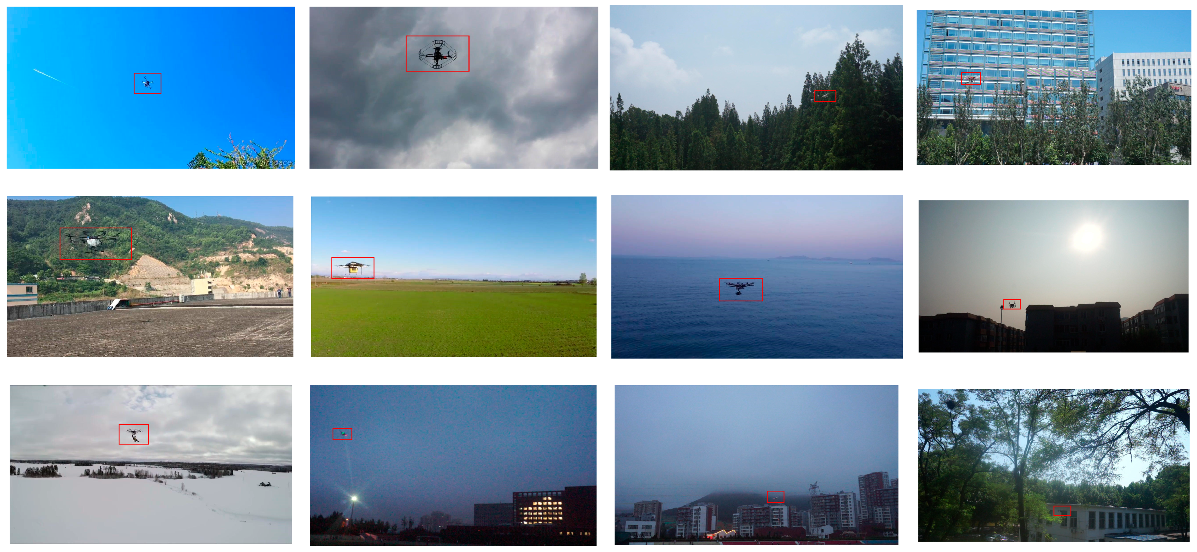Specifically, the annotated targets cover less than 0.05 of the image area, with an overall mean area ratio of 0.0031, a maximum of 0.045, and a minimum of 2.7 × 10⁻⁴. The scenes include sky, buildings, jungles, and farmlands. Lighting conditions cover daytime, dusk, and night; weather involves sunny, cloudy, and snowy days. This diversity makes the dataset a challenging testbed for small-object detection in complex environments. Some examples of the dataset are shown in Figure 7.

For a holistic evaluation of the model, this paper adopts the following metrics from two dimensions: accuracy and efficiency.

The accuracy metrics adopted here include precision (P), recall (R), the F1-score, and mean average precision at IoU thresholds of 0.5 and 0.5:0.95 (mAP@0.5 and mAP@0.5:0.95). In this task, positive samples are real UAV targets, and negative samples are backgrounds or other non-UAV regions. Precision indicates how many of the predicted UAV boxes are correct, while recall indicates how many of the ground-truth UAVs are found. Formally, they are defined as follows:

$$\mathrm{P}={\displaystyle \frac{\mathrm{T}\mathrm{P}}{\mathrm{T}\mathrm{P}+\mathrm{F}\mathrm{P}}}$$

(8)

$$\mathrm{R}={\displaystyle \frac{\mathrm{T}\mathrm{P}}{\mathrm{T}\mathrm{P}+\mathrm{F}\mathrm{N}}}$$

(9)

where TP stands for the count of genuine UAVs that are successfully detected, FP represents the count of non-UAV items (backgrounds or other objects) that are wrongly classified as UAVs, and FN indicates the count of real UAVs that escape detection. The F1-score is subsequently calculated as the harmonic mean of precision and recall:

$$\mathrm{F}1=2\times {\displaystyle \frac{\mathrm{P}\times \mathrm{R}}{\mathrm{P}+\mathrm{R}}}$$

(10)

mAP@0.5 corresponds to the average precision when the IoU threshold is fixed at 0.5. By contrast, mAP@0.5:0.95 is obtained by averaging the average precision scores over ten thresholds that increase from 0.5 to 0.95 in steps of 0.05. For small low-altitude UAV targets, a slight offset in the predicted box can cause a substantial change in IoU; therefore, mAP@0.5:0.95 provides a stricter evaluation of the model’s actual performance in fine localization.

The efficiency of the model is quantified by three indicators: the number of parameters (which measures storage footprint), GFLOPs (which measures computational complexity), and FPS (which measures inference speed).

4.2. Experimental Environment and Setup

A fixed hardware and software environment was maintained throughout all experiments to ensure reproducibility. The detailed configurations are listed in

Table 1. Experimental environment configuration.

Item	Configuration Details
CPU	AMD Ryzen 9 7940H w/Radeon 780M Graphics
GPU	NVIDIA GeForce RTX 4060
Memory	16GB
Storage	SSD 512G
Operating System	Windows 11
PyTorch Version	2.2.0 + cu118
Python Version	3.9.25
CUDA Version	11.8

Note: AMD (Santa Clara, CA, USA); NVIDIA (Santa Clara, CA, USA); Windows 11 (Redmond, WA, USA); PyTorch (Menlo Park, CA, USA); Python (Beaverton, OR, USA); CUDA (Santa Clara, CA, USA).

.

All input images are uniformly resized to 640 × 640 pixels. All experiments are conducted under a unified training protocol to ensure fair comparisons. The optimizer is configured as Stochastic Gradient Descent (SGD) with a momentum of 0.937 and a weight decay of 0.0005. The initial learning rate is set to 0.01 and decays to 0.0001 at the end of training following a linear decay schedule, with a warm-up period of three epochs (warm-up momentum of 0.8). The batch size is set to eight, and the total number of training epochs is 200. For data augmentation, we apply mosaic augmentation, horizontal flipping, HSV color-space adjustments (hue, saturation, and value), and random scaling and translation with standard YOLO parameters. Mosaic augmentation is disabled during the final 10 epochs to stabilize training. Mixed precision training is enabled to accelerate computation and reduce GPU memory consumption. The confidence threshold for detection is set to 0.25, and the non-maximum suppression (NMS) IoU threshold is 0.45. These hyperparameter settings are summarized in

Table 2. Hyperparameter settings.

Hyperparameter	Value
Batch size	8
Image size	640 × 640
Number of epochs	200
Initial learning rate	0.01
Optimizer	SGD
Learning rate schedule	Linear decay with 3-epoch warm-up
Data augmentation	Mosaic, HSV, flipping, scaling, translation
Confidence threshold	0.25
NMS IoU threshold	0.45
Mixed precision	True

.

4.3. Ablation Experiments

To evaluate the contribution of each proposed module, we conduct ablation experiments on the DUT Anti-UAV dataset, starting from the original YOLOv11 as the baseline. The results are summarized in

Table 3. Ablation experiment results.

Model	F1	P	R	mAP@0.5	mAP@0.5:0.95	Parameter (M)	GFLOPs
Baseline	89.71	95.6	84.5	89.6	58.4	2.58	6.3
Baseline + WIoU V3	90.77	97.0	85.3	91.1	58.9	2.58	6.3
Baseline + C3k2_SCSA	90.29	96.4	84.9	90.3	59.0	2.67	6.8
Baseline + DySample	89.69	96.6	83.7	89.8	58.0	2.56	6.3
Baseline + P2 Head	91.83	96.6	87.5	91.9	61.0	1.94	9.7
Baseline + C3k2_SCSA + P2 Head	92.14	97.3	87.5	92.1	61.4	2.11	11.0
Baseline + DySample + P2 Head	92.15	97.2	87.6	91.9	61.5	1.94	9.7
Baseline + C3k2_SCSA + DySample + P2 Head	90.94	96.1	86.3	91.0	60.5	2.11	11.0
Ours (All)	92.26	96.6	88.3	92.2	61.5	2.11	11.0

.

(a)

Single-module analysis. Replacing the standard IoU loss with WIoU v3 pushes precision from 95.6% to 97.0% and lifts mAP@0.5 by 1.5 points, without adding a single parameter. This suggests that its dynamic non-monotonic focusing effectively dials down the influence of low-quality samples during training. The C3k2_SCSA module improves precision to 96.4% and mAP@0.5 to 90.3% with only a 0.09 M increase in parameters, showing that channel-spatial attention can strengthen small-target discrimination and suppress background clutter at a negligible cost. DySample alone raises precision by 1.0 point but slightly reduces recall (84.5% → 83.7%), indicating that dynamic upsampling by itself, without complementary attention guidance or detection head adjustments, does not yet translate into better recall for the smallest targets. The P2 head produces the largest single-module gain: Recall jumps from 84.5% to 87.5%, and both mAP@0.5 and mAP@0.5:0.95 rise by over 2 points, while the parameter count drops to 1.94 M. This confirms that shallow high-resolution features are critical for localizing extremely small drones, and that removing the mostly idle P5 head trims the model without hurting performance.

(b)

Multi-module analysis. Pairing C3k2_SCSA with the P2 head pushes precision to 97.3% and mAP@0.5 to 92.1%, outperforming either module alone. This points to a genuine synergy: the attention module helps the high-resolution head focus on the right features, and the head gives those features a direct path to the detection decision. DySample combined with the P2 head achieves the highest mAP@0.5:0.95 (61.5%) among the two-module variants, suggesting that content-aware upsampling preserves edge details that complement the head’s fine-grained localization capability. A noteworthy result emerges when C3k2_SCSA, DySample, and the P2 head are integrated together without WIoU v3: all metrics decline compared to the two-module setups, with recall dropping from 87.5–87.6% to 86.3% and mAP@0.5:0.95 falling from 61.4–61.5% to 60.5%. Rather than attributing this to overfitting, we suspect a feature-level interference effect. SCSA suppresses background responses, which may weaken the gradient cues that DySample uses to predict sampling offsets; conversely, DySample’s content-adaptive resampling can shift the spatial distribution that subsequent SCSA layers are designed to process. When these two modules are naïvely superimposed, their modifications to the feature space appear to work against each other. Adding WIoU v3 to the full model resolves this degradation (mAP@0.5:0.95 recovers from 60.5% to 61.5%, and recall from 86.3% to 88.3%), suggesting that its outlier-aware gradient allocation absorbs some of the training instability introduced by simultaneously reshaping features through attention and dynamic upsampling.

(c)

Full model. The complete model achieves an F1-score of 92.26, precision of 96.6%, recall of 88.3%, mAP@0.5 of 92.2%, and mAP@0.5:0.95 of 61.5%, with 2.11 M parameters. Compared with the baseline, recall improves by 3.8 points, mAP@0.5 and mAP@0.5:0.95 rise by 2.6 and 3.1 points, respectively, and the parameter count drops by 18.2%. Taken together, the P2 head supplies the fine-grained spatial detail that small targets depend on, C3k2_SCSA sharpens what the model attends to, DySample keeps object boundaries from blurring during upsampling, and WIoU v3 keeps the training signal clean. The four modules complement rather than compete with each other, yielding a detector that pushes small-target accuracy up while staying compact.

4.4. Loss Function Comparison Analysis

To isolate the effect of the loss function, we compare GIoU [34], DIoU [35], Efficient-IoU (EIoU) [36], and WIoU v3 on the baseline YOLOv11 model under identical training settings, using the default CIoU as the reference. The results are reported in

Table 4. Performance comparison of different loss functions on the baseline model.

Loss Function	F1	P	R	mAP@0.5	mAP@0.5:0.95
CIoU	89.71	95.6	84.5	89.6	58.4
GIoU	89.90	96.7	84.0	89.6	58.2
DIoU	90.38	96.1	85.3	90.1	59.3
EIoU	89.27	95.9	83.5	89.3	58.1
WIoU v3	90.77	97.0	85.3	91.1	58.9

.

WIoU v3 achieves the highest precision (97.0%), mAP@0.5 (91.1%), and F1-score (90.77) among all five loss functions, outperforming CIoU by 1.4, 1.5, and 1.06 points, respectively. Its recall (85.3%) matches DIoU’s, and its mAP@0.5:0.95 (58.9%) trails DIoU’s 59.3% by just 0.4 points. DIoU, while slightly ahead on the stricter metric, falls short on precision (96.1%) and mAP@0.5 (90.1%).

In low-altitude anti-UAV detection, a false positive can be far more disruptive than a slightly imprecise bounding box. Mistaking background clutter for a UAV triggers unnecessary alerts, while a box that is off by a few pixels on a real drone is still actionable. WIoU v3 delivers a clear precision advantage over DIoU (+0.9 points) and a substantial mAP@0.5 lead (+1.0 point), indicating that it keeps false alarms lower while maintaining the same detection coverage. The small 0.4-point gap in mAP@0.5:0.95 is consistent with how WIoU v3 works. Unlike DIoU, which applies a uniform center-point penalty to all anchor boxes regardless of quality, WIoU v3 introduces a dynamic non-monotonic focusing mechanism that assigns differentiated gradient gains based on sample quality. Samples with imprecise boundaries, such as motion-blurred or heavily occluded small drones, receive reduced optimization pressure, preventing the model from overfitting to noisy annotations. Conversely, anchor boxes with reliable labels receive sufficient gradient updates to ensure accurate localization. This selective allocation of gradient gains leads to cleaner predictions with fewer false positives, at the cost of a slight relaxation in strict IoU localization. The model simply invests less optimization effort on boxes whose ground-truth coordinates are uncertain. This trade-off accepts a slight relaxation in strict IoU localization in exchange for markedly cleaner predictions, a sensible choice for this deployment context. DIoU’s marginally higher mAP@0.5:0.95 does not contradict this interpretation. It confirms that WIoU v3 is making the trade-off it was designed to make.

Among the remaining losses, GIoU records the lowest recall at 84.0%. EIoU delivers the weakest recall and mAP@0.5:0.95. Its precision (95.9%) is slightly above CIoU, but this does not translate into competitive overall performance. One possible explanation is that the extra geometric terms EIoU introduces offer limited benefit when targets are extremely small, and their aspect ratios vary little across the dataset. These terms capture aspect ratio and side-length consistency, which may simply not carry enough signal for tiny objects. Across all five loss functions, WIoU v3 gives the cleanest trade-off between catching small drones and avoiding false positives.

4.5. Analysis of the DySample Module

DySample’s behavior is controlled by two parameters: the number of groups G and the static range factor λ. G determines how channels are partitioned during offset generation, while λ caps the magnitude of sampling-point offsets relative to the initial grid. We determine both through controlled-variable experiments on the complete model.

(a)

Effect of the number of groups G. Fixing λ = 0.25, G is gradually increased from 1 to 5, and the results are shown in

Table 5. Performance of DySample under different group numbers G.

Number of Groups G	F1	P	R	mAP@0.5	mAP@0.5:0.95
G = 1	91.95	96.4	87.9	92.0	59.2
G = 2	91.80	95.7	88.2	92.1	59.4
G = 3	92.12	97.0	87.7	92.1	59.5
G = 4	92.26	96.6	88.3	92.2	61.5
G = 5	92.15	96.6	88.1	92.1	59.2

.

The model performs best at G = 4: mAP@0.5 reaches 92.2%, mAP@0.5:0.95 climbs to 61.5%, and the F1-score of 92.26 is the highest across all five settings. As G goes from 1 to 4, mAP@0.5:0.95 rises steadily from 59.2% to 61.5%. Finer channel grouping gives the offset generation branches more diverse views of the feature map, so sampling points can adapt to edges across different spatial regions more flexibly. When G is pushed to 5, mAP@0.5:0.95 drops back to 59.2%, and F1-score falls to 92.15. Beyond a certain point, more groups appear to introduce redundancy rather than useful diversity, which hurts stable learning of the sampling coordinates.

At G = 3, precision peaks at 97.0%, but mAP@0.5:0.95 sits at only 59.5%, well below the 61.5% at G = 4. This gap suggests that the sampling strategy at G = 3 helps the model filter out false positives very effectively, but the boxes it keeps do not align as tightly with the ground truth. Moving to G = 4 trades 0.4 points of precision for a large jump in mAP@0.5:0.95. The localization gain from richer sampling diversity clearly outweighs the small drop in precision.

(b)

Effect of the static range factor λ. Fixing G = 4, we vary λ from 0 to 0.45. The results are shown in

Table 6. Performance of DySample under different static range factors λ (G = 4).

λ	F1	P	R	mAP@0.5	mAP@0.5:0.95
0	91.90	96.4	87.8	92.0	59.7
0.15	91.73	96.2	87.7	91.8	59.5
0.25	92.26	96.6	88.3	92.2	61.5
0.35	91.83	96.0	88.0	91.7	59.6
0.45	91.98	96.1	88.2	92.0	59.5

.

The static range factor λ has a pronounced effect on accuracy, and the trend is a clear rise to a peak followed by a decline. Performance is best at λ = 0.25, where mAP@0.5:0.95 reaches 61.5% and mAP@0.5 hits 92.2%.

When λ is small (0 to 0.15), the sampling offsets are tightly constrained. DySample barely moves away from bilinear interpolation, so its content-awareness is not fully used. mAP@0.5:0.95 drops by roughly 1.8 to 2.0 points relative to the optimum. At the other end (0.35 to 0.45), the offsets become too large. Some sampling points drift toward background noise instead of staying on the target, pulling mAP@0.5 down to 91.7–92.0% and mAP@0.5:0.95 down to 59.5–59.6%.

For low-altitude anti-UAV targets, the boundary between a small drone and background clutter is fragile. The gradient cues at object contours are weak and easily mixed with surrounding texture. This makes precise control of the offset range especially important: too little range wastes the benefit of dynamic sampling, while too much range cancels out the edge-preservation advantage because the sampling points wander. A setting of λ = 0.25 sits in the middle, where the offset is large enough to adapt to object boundaries but not so large that it gets pulled off target.

In terms of metric sensitivity differences, mAP@0.5 only requires IoU ≥ 0.5 and is relatively tolerant of fine-grained bounding box offsets. In contrast, mAP@0.5:0.95 is an average of multiple strict IoU thresholds and is highly sensitive to localization accuracy. The number of groups G and the range factor λ in DySample essentially adjust the precision of the spatial distribution of the sampling points. This primarily improves the fine-grained localization of bounding boxes (e.g., correcting minor offsets), thereby significantly boosting mAP at high IoU thresholds while offering limited improvement for coarse localization (IoU = 0.5). Therefore, the consistent performance of mAP@0.5 is a reasonable and expected outcome given the underlying technical principles.

Combining the two sets of experiments, we fix DySample at $G=4$ and $\lambda =0.25$ for the final model. This configuration leads the other parameter choices by a clear margin on the strict mAP@0.5:0.95 metric.

4.6. Comparison Analysis with Other Mainstream Models

A comparison of the proposed method against several mainstream lightweight detectors is performed on the DUT Anti-UAV test set. The compared models include YOLOv5n, YOLOv8n, YOLOv10n, YOLOv11n, YOLOv12n, and YOLOv26n, all used in their official nano versions. Training and evaluation are carried out under the same hardware environment, hyperparameter settings, and input size (640 × 640).

Table 7. Comparison results with mainstream detection models.

Model	F1	P	R	mAP@0.5	mAP@0.5:0.95	Parameters (M)	GFLOPs
YOLOv5n	89.84	96.3	84.2	89.5	57.9	2.50	7.1
YOLOv8n	90.09	95.2	85.5	89.7	58.4	3.01	8.1
YOLOv10n	89.30	94.8	84.4	89.5	57.9	2.27	6.5
YOLOv11n	89.71	95.6	84.5	89.6	58.4	2.58	6.3
YOLOv12n	89.54	94.6	85.0	89.4	58.0	2.56	6.3
YOLOv26n	91.29	95.3	87.6	91.9	61.1	2.38	5.2
Ours	92.26	96.6	88.3	92.2	61.5	2.11	11.0

summarizes the results.

Our model leads all competitors on every accuracy metric. Precision reaches 96.6% and recall 88.3%, surpassing the baseline YOLOv11n by 1.0 and 3.8 points, respectively. These gains show that the model has become both better at telling small drones from background clutter and less prone to missing them altogether. mAP@0.5:0.95 reaches 61.5%, 3.1 points above the baseline, while the parameter count drops to 2.11 M, an 18.2% reduction. Against the other YOLO nano-variants, our model holds the lowest parameter count and outperforms YOLOv5n, YOLOv8n, YOLOv10n, YOLOv12n, and YOLOv26n by margins of 2.7, 2.5, 2.7, 2.8, and 0.3 points in mAP@0.5, and by 3.6, 3.1, 3.6, 3.5, and 0.4 points in mAP@0.5:0.95. The stricter the IoU threshold, the wider the gap becomes. This widening gap under strict IoU thresholds is consistent with the expectation that the P2 head and DySample jointly improve fine localization.

Our model’s GFLOPs (11.0) are higher than those of the other nano-variants. This is a direct consequence of the P2 detection head, which operates on shallow feature maps of substantially higher spatial resolution than the P3 and P4 layers. The ablation results already confirm this attribution: adding the P2 head alone raises GFLOPs from 6.3 to 9.7. In return, that same P2 head, together with DySample, delivers the largest gains in mAP@0.5:0.95 and recall among all our design modifications. The trade is therefore explicit: a manageable increase in computation for a decisive improvement in small-target localization. Thanks to the removal of the P5 head and the negligible overhead of DySample, the total parameter count remains the lowest of all compared models, confirming that our model is parameter-efficient despite its higher GFLOPs.

In addition to the YOLO series, several specialized anti-UAV detectors have been proposed and evaluated on the DUT Anti-UAV dataset.

Table 8. Comparison with state-of-the-art specialized anti-UAV detectors on the DUT Anti-UAV dataset.

Model	P	R	mAP@0.5	mAP@0.5:0.95
DRBD-YOLOv8 [17]	90.9	77.0	85.7	53.5
DRF-YOLO [37]	93.9	80.3	86.9	54.8
Ours	96.6	88.3	92.2	61.5

compares our method with two representative approaches that report publicly available results on this benchmark.

DRBD-YOLOv8 introduces depthwise separable convolutions, an RCELAN module, a BiFPN architecture, and a DN-ShapeIoU loss function to achieve a lightweight and efficient anti-UAV detector. DRF-YOLO incorporates a dilated-wise residual (DWR) module and an asymptotic feature pyramid network (AFPN) to enhance contextual representation and multi-scale feature fusion. On the DUT Anti-UAV dataset, these methods achieve 85.7% and 86.9% mAP@0.5, respectively, with corresponding mAP@0.5:0.95 of 53.5% and 54.8%. In comparison, our method attains 92.2% mAP@0.5 and 61.5% mAP@0.5:0.95 with only 2.11 M parameters, outperforming both approaches by substantial margins across all metrics. It should be noted that direct numerical comparisons are subject to differences in training configurations and hardware implementations. Nevertheless, the consistent improvements suggest that our method provides a competitive solution for anti-UAV detection tasks.

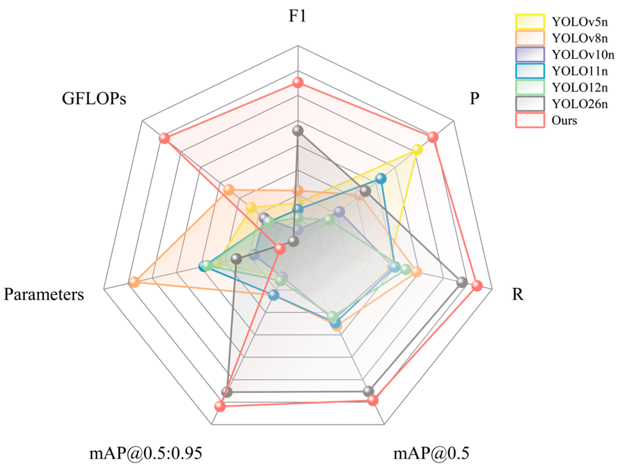
Figure 8 presents a radar chart comparing all models across seven dimensions: F1, P, R, mAP@0.5, mAP@0.5:0.95, GFLOPs, and parameter count. Our model forms the largest envelope on the accuracy axes while staying tight on parameter count, giving a clear visual summary of the accuracy–efficiency balance it achieves.

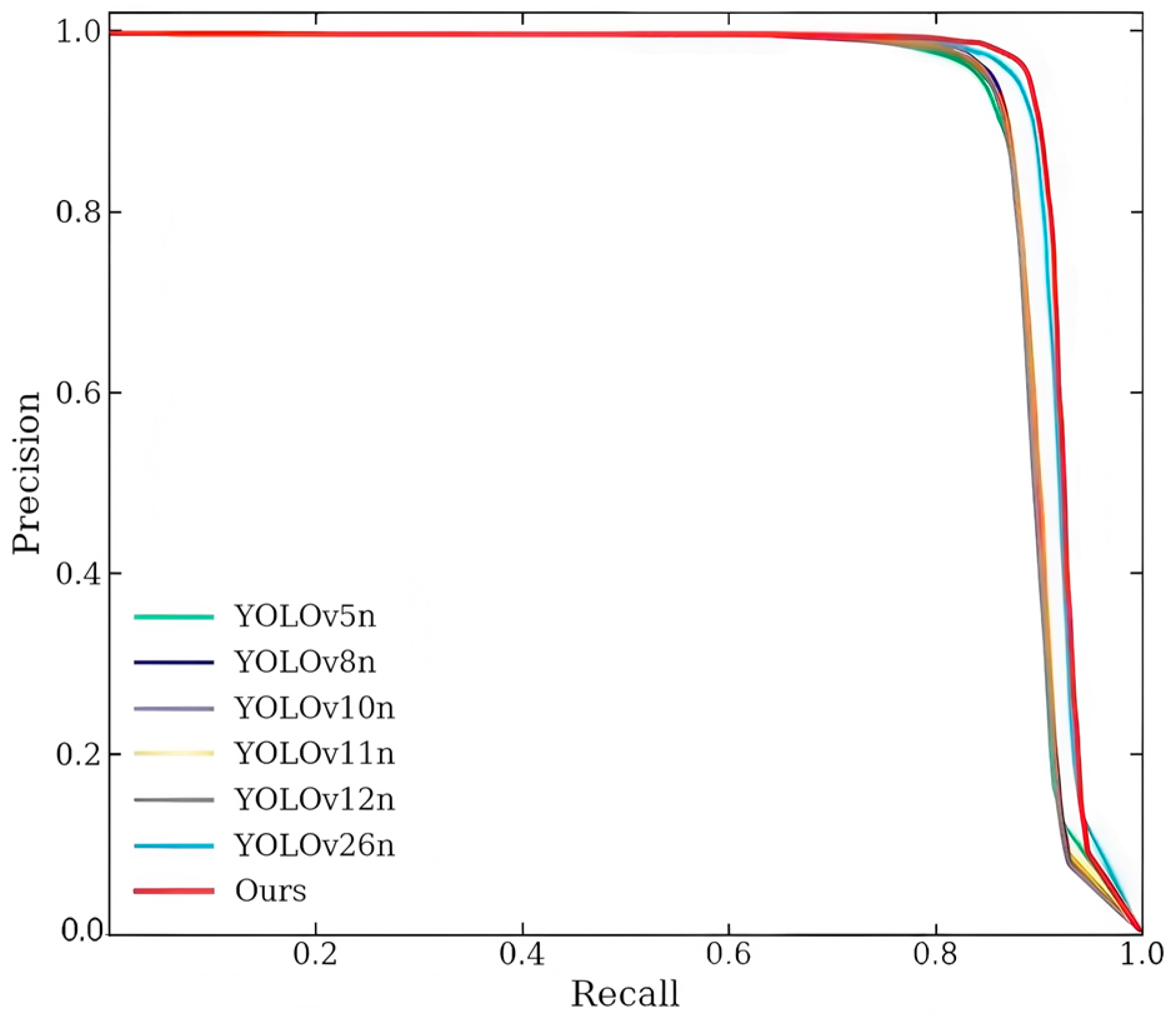
The precision–recall curves for all compared models are consolidated in Figure 9. Our model’s curve encloses the largest area and maintains high precision across the full recall range. This matches the F1 ranking in Table 7, where our model reaches 92.26 and the others fall between 89 and 91.

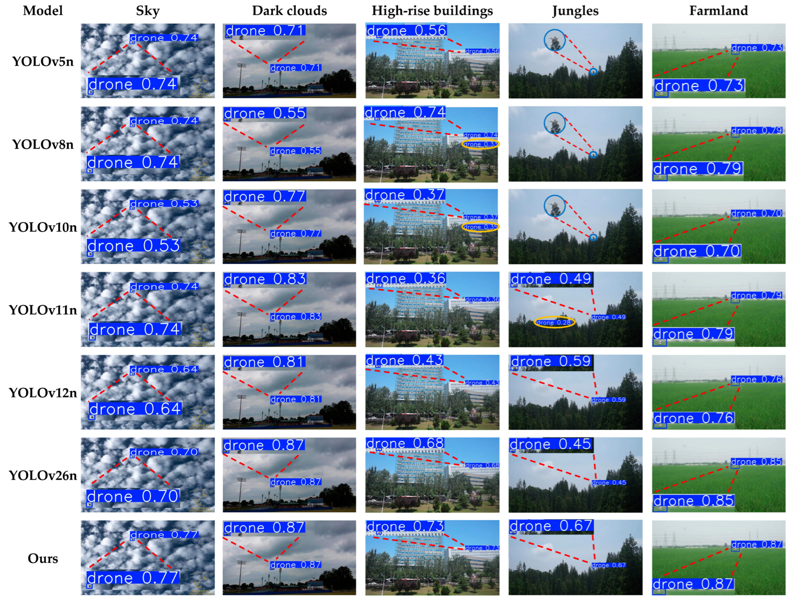
To see how these numerical differences translate into real detection behavior, we pick representative images from the DUT Anti-UAV test set that cover challenging conditions: complex backgrounds (sky, dark clouds, high-rise buildings, jungles, and farmland), long-range tiny targets, varying illumination, and partial occlusion. To improve the interpretability of the visual comparisons, we provide local zoom-in patches for each detection example, clearly showing the target regions and the corresponding detection results. False detections are highlighted with orange ellipses for easy identification. We visually compare our model against the YOLOv11n baseline, with YOLOv5n, YOLOv8n, YOLOv10n, YOLOv12n, and YOLOv26n shown alongside as horizontal references. Figure 10 displays the results. Each row corresponds to a model, and each column to a scene.

In relatively clean backgrounds such as sky, dark clouds, and farmland, all models detect the drone, but our model consistently outputs higher confidence scores. The differences become sharper in texture-rich scenes. In the high-rise building scene, both YOLOv8n and YOLOv10n produce false positives on building edges, while our model does not. In the jungle scene, the target is partially hidden by tree canopies and extremely small. YOLOv5n, YOLOv8n, and YOLOv10n miss it entirely, and YOLOv11n mistakes a branch for the drone. Our model detects the target correctly, with a confidence of 0.67. Taken together, these visual comparisons show the combined effect of our design choices: C3k2_SCSA’s background suppression, DySample’s edge preservation, and the P2 head’s direct access to shallow fine-grained features all contribute to cleaner detection in complex scenes.

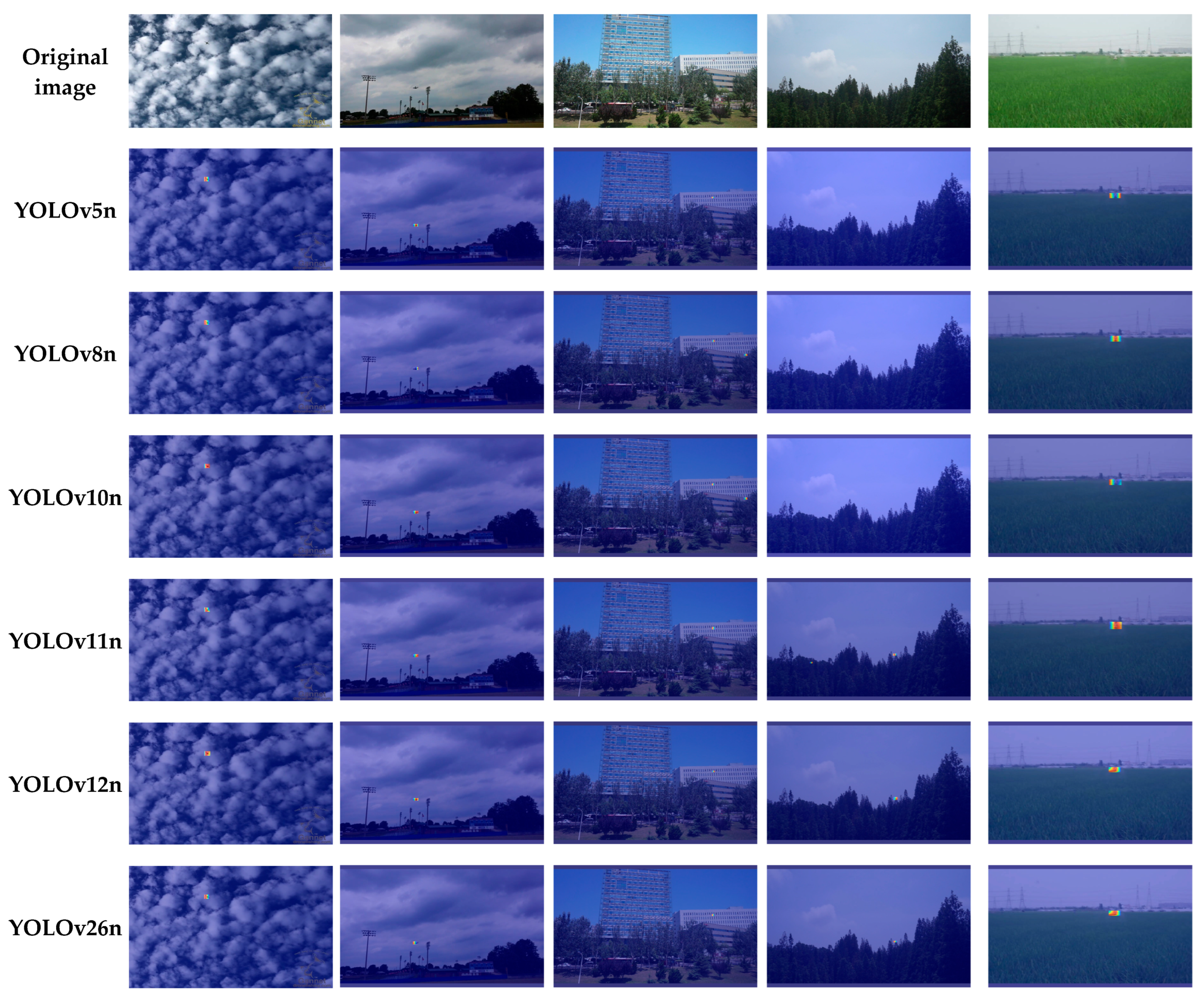
To further examine where the model directs its attention, we use Grad-CAM to visualize the output of the last backbone layer. The results are shown in Figure 11. In the baseline model, the activation regions spread diffusely, with many high-response patches falling on background elements such as tree canopies and roof edges. The model’s discriminative features are visibly diluted by background information. In our model, the heatmaps tighten around the drone contours and their immediate surroundings, while background responses are strongly suppressed. This side-by-side comparison shows directly how C3k2_SCSA’s attention mechanism refocuses the model away from clutter and onto the target, even when the scene is visually busy.

4.7. Cross-Dataset Evaluation

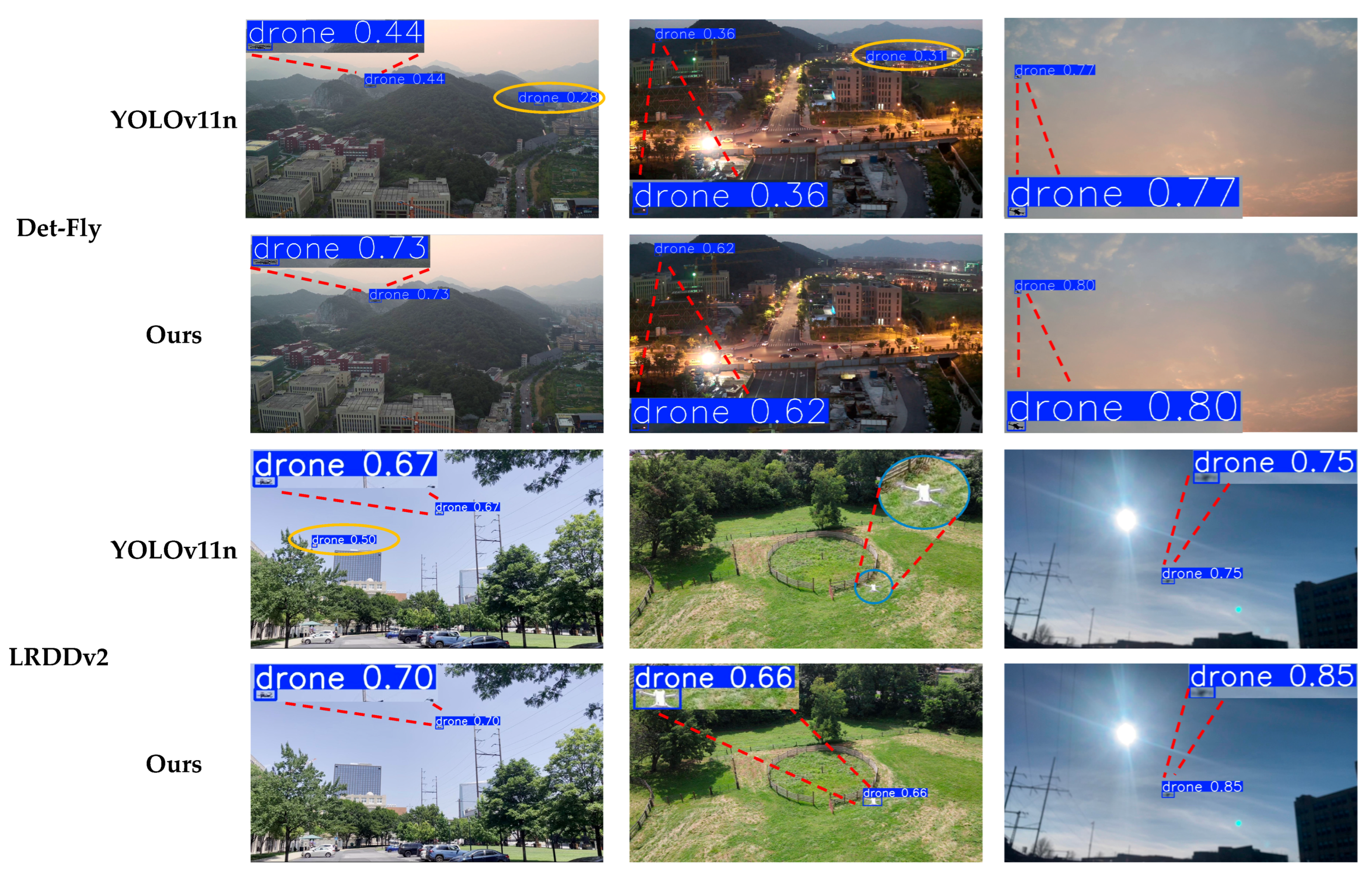
To test generalization beyond the main dataset, we conduct cross-dataset evaluation on two public UAV detection datasets: Det-Fly and LRDDv2. From each, 1000 images are selected (2000 total), and none of these images appear in any training set—they are used exclusively for testing. Det-Fly emphasizes small UAVs against cluttered backgrounds such as trees and buildings, while LRDDv2 covers low-altitude targets under diverse illumination and weather. Both datasets are converted to the YOLO annotation format, with images resized to 640 × 640.

Table 9. Cross-dataset evaluation results.

Dataset	Model	P	R	F1	mAP@0.5	mAP@0.5:0.95
Det-Fly	YOLOv11n	88.63	60.40	71.84	67.13	37.67
	Ours	92.32	66.15	77.07	71.95	42.04
LRDDV2	YOLOv11n	83.82	61.25	70.78	65.67	34.12
	Ours	86.49	65.07	74.26	69.51	38.58

reports the results.

On Det-Fly, where trees and buildings create substantial background clutter, our model improves precision by 3.69 points (to 92.32%) and recall by 5.75 points (to 66.15%). mAP@0.5 rises from 67.13% to 71.95%, and mAP@0.5:0.95 climbs from 37.67% to 42.04%. The gains in recall and mAP@0.5:0.95 are particularly telling: Det-Fly’s background interference is exactly the kind of challenge that SCSA and DySample were designed to handle, and the numbers bear this out.

On LRDDv2, which stresses models with varied illumination and weather, our model again improves consistently. Precision reaches 86.49% (+2.67 points), recall 65.07% (+3.82 points), mAP@0.5 69.51% (+3.84 points), and mAP@0.5:0.95 38.58% (+4.46 points). The 4.46-point lift in mAP@0.5:0.95 is the largest relative gain across both datasets, suggesting that WIoU v3’s handling of low-quality samples and the P2 head’s access to fine-grained features together strengthen the model when image quality degrades.

Across two datasets with different scene types and data distributions, our model consistently outperforms the baseline. No component was tuned on either Det-Fly or LRDDv2; the gains transfer directly, which supports the claim that the proposed modules confer genuine generalization rather than dataset-specific fitting.

Figure 12 shows representative detection results from both datasets, with local zoom-in patches provided for each example to clearly visualize the target regions. False detections are highlighted with orange ellipses for easy identification. On Det-Fly, the baseline model produces two false positives, both linked to the combination of a cluttered background and insufficient lighting. Our model avoids these errors. On LRDDv2, the baseline misses one target and produces one false positive. The missed target is washed out by strong light against a complex background. The false positive occurs where a branch or similarly shaped occlusion is mistaken for a target. Across all examples, our model also outputs higher confidence scores on correctly detected targets. These observations are consistent with the numerical trends in Table 8: the recall improvements on Det-Fly and the precision gains on LRDDv2 both have visible counterparts in the detection outputs.

4.8. Edge Device Deployment Experiments

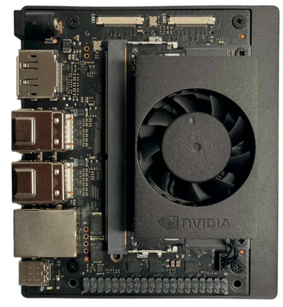
The NVIDIA Jetson Orin Nano Super(NVIDIA, Santa Clara, CA, USA) is used as the test platform. With a 1024-core Ampere GPU and 8 GB of LPDDR5 memory, it represents a typical high-efficiency edge computing device for embedded real-time detection tasks. The power mode is set to 15 W. The device is shown in Figure 13.

Both the baseline YOLOv11n and our final model are optimized via TensorRT with FP16 half-precision, at a fixed input size of 640 × 640. The test set consists of 2200 images from the DUT Anti-UAV dataset, and each measurement is averaged over five consecutive inference runs. The metrics reported include model forward inference latency (core inference only), end-to-end frame rate (covering image reading, preprocessing, inference, and postprocessing), and peak GPU memory usage. Results are shown in

Table 10. Edge device deployment performance.

Model	Inference Latency (ms)	End-to-End FPS	Memory Usage (MB)	TensorRT Engine Size (MB)
YOLOv11n	4.35	45.21	144	8.3
Ours	8.91	37.35	155	7.9

.

Under TensorRT FP16, our model runs at 8.91 ms inference latency and 37.35 end-to-end FPS, well above the real-time threshold of 30 FPS. Peak GPU memory usage is 155 MB, and the serialized engine occupies only 7.9 MB on disk. Note that the engine file size reflects only offline storage; runtime GPU memory also accommodates weights and feature maps, which accounts for the larger figures in Table 10. Compared with the baseline, our model’s frame rate drops by roughly 17.4%. This is the trade-off for the accuracy gains reported in Section 4.6: a model that is better at finding small drones, at the expense of running slightly slower. For anti-UAV deployment, where missing a target is far costlier than processing a few frames slower, 37 FPS is comfortably above the real-time threshold and leaves enough headroom for practical use.

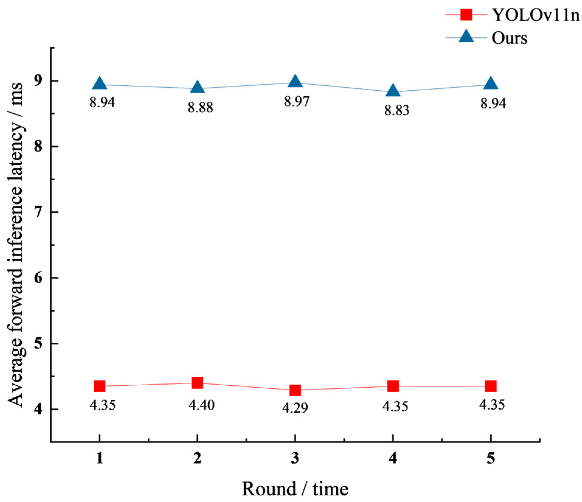
To assess inference time stability, we record single-frame forward latency over five consecutive runs. The results appear in Figure 14. The baseline YOLOv11n latency stays around 4.35 ms (range: 4.29–4.40 ms), while our model’s latency remains near 8.91 ms (range: 8.83–8.97 ms). In both cases, the per-run fluctuation stays within 0.15 ms. For a real-time detection pipeline running at 37–45 FPS, this level of jitter is negligible.

With 2.11 M parameters and a 7.9 MB TensorRT engine, the proposed model loads and runs stably on a resource-constrained Jetson Orin Nano Super at 37 FPS. This confirms that the accuracy gains demonstrated in earlier sections do not come at the expense of deployability.

5. Discussion

The ablation results reveal a pattern that goes beyond individual module performance: these modules are not additive in a simple way. DySample alone raises precision but lowers recall. C3k2_SCSA, DySample, and the P2 head together, without WIoU v3, perform worse than two-module combinations. Yet the full four-module model achieves the best results across all metrics. What emerges is a conditional synergy. DySample’s content-aware sampling needs attention guidance to avoid drifting toward strong but irrelevant gradients. SCSA’s background suppression and DySample’s spatial resampling, when superimposed, can interfere with each other in the feature space unless the training signal is stabilized. WIoU v3 provides that stabilization by down-weighting unreliable samples. The four modules do not simply add up; they require each other to function as intended. This carries a practical implication for lightweight detector design: when several feature-space modifications are introduced simultaneously, a matched training strategy is not optional. It is what allows the modifications to cooperate rather than compete.

Two aspects distinguish this work from most existing anti-UAV detectors. First, the core modules, SCSA and DySample, are designed under a near-zero parameter budget, relying on global pooling, lightweight convolutions, and linear offset generation. Second, the four improvements form a complete design chain rather than a collection of isolated optimizations. The ablation results, where module combinations behave differently from individual modules, provide experimental support for this system-level approach. Direct numerical comparison with published anti-UAV methods is difficult because few report results on DUT Anti-UAV. Our comparative evaluation therefore focused on the YOLO nano-series, which offers a consistent and reproducible baseline across multiple versions.

Despite the promising results, several limitations of this study should be acknowledged. First, while our evaluation covers snowy and cloudy conditions, it does not include high-moisture extreme weather such as heavy rain and thick fog. These conditions introduce strong optical scattering that can fundamentally degrade image contrast and edge information, posing a distinct challenge to the SCSA mechanism and the DySample dynamic upsampling pipeline. Building a multi-weather dataset and systematically assessing model robustness under such conditions is a concrete direction for our immediate future work. Second, this study focuses on single and sparse UAV targets. As noted in the ablation analysis, dense UAV swarms introduce fundamentally different challenges—including severe mutual occlusion, similar appearance, and overlapping bounding boxes—that the current model architecture is not designed to handle. Extending the proposed approach to swarm scenarios, potentially through multi-object tracking integration or swarm-specific detection heads, represents an important avenue for subsequent research. Third, the current cross-dataset evaluation is limited to two additional datasets (Det-Fly and LRDDv2). Expanding the evaluation to more diverse platforms, altitudes, and background environments would further validate the generalizability of our design.

6. Conclusions

This paper presented a lightweight detection method for low-altitude anti-UAV scenarios, built on YOLOv11n. Four targeted modifications were introduced: the SCSA mechanism for background suppression, DySample dynamic upsampling for edge preservation, and a restructured detection head that focuses on the P2 small-object branch, together with the WIoU v3 loss designed to ensure robust training. Together, these changes push detection accuracy up while keeping the model compact.

On the DUT Anti-UAV dataset, the proposed detector yields 92.2% mAP@0.5 and 61.5% mAP@0.5:0.95 with a mere 2.11 M parameters, thereby outperforming YOLOv11n and several other nano-scale YOLO variants. Cross-dataset evaluation on Det-Fly and LRDDv2 confirms that the gains transfer to different scenes and data distributions. After TensorRT FP16 optimization on a Jetson Orin Nano Super, the model runs at 37 FPS end-to-end with 155 MB of GPU memory and a 7.9 MB engine file, meeting the real-time requirement for practical surveillance tasks.