Toward a Deeper Understanding of YOLO26: Block-Level Architectural Analysis and Ablation Studies

Abstract

Public YOLO model releases typically provide high-level architectural descriptions and headline benchmark results but offer limited empirical attribution of performance to individual blocks under controlled training conditions. This paper presents a modular, block-level analysis of YOLO26’s object detection architecture, detailing the design, function, and contribution of each component. We systematically examine YOLO26’s convolutional modules, bottleneck-based refinement blocks, spatial pyramid pooling, and position-sensitive attention mechanisms. Each block is analyzed in terms of objective and internal flow. In parallel, we conduct targeted ablation studies to quantify the effect of key design choices on accuracy (mAP@0.50:0.95) and inference latency under a fixed seed-0, COCO-only, fully specified training and benchmarking protocol. Experiments use the MS COCOdataset with the standard train2017 split (≈118 k images) for training and the full val2017 split (5 k images) for evaluation. The result is a self-contained empirical architectural-attribution reference that supports interpretability, reproducibility, and evidence-based architectural decision-making for real-time detection models. Beyond isolated ablations, we further synthesize the best-performing design choices into combined YOLO26n configurations and compare them against the default baseline. The best combined configuration improves mAP@0.50:0.95 from 0.3933 to 0.3969, while introducing only a marginal latency increase from 0.99 ms to 1.00 ms under TensorRT FP16 benchmarking. This analysis identifies an improved accuracy–latency trade-off and provides an incremental architectural configuration contribution supported by controlled experiments. The study is, therefore, framed as a controlled empirical analysis and configuration-refinement study of YOLO26, rather than as the proposal of a new detector family or a claim of universal detector superiority.

1. Introduction

Object detection has advanced rapidly over the past decade, with one-stage detectors such as the YOLO (You Only Look Once) family [1,2,3,4,5,6,7,8,9,10,11,12] offering a practical balance of detection accuracy and inference speed for real-time computer vision applications. In this context, the question of which YOLO version is ‘best’ is rarely absolute or deployment-independent. It is typically framed as a trade-off between detection accuracy and inference speed. Prior studies and surveys emphasize that no single detector universally dominates across datasets [13,14,15], tasks, deployment backends, and evaluation settings, and that reported improvements can be sensitive to training recipes, checkpoint assumptions, and benchmarking assumptions. The Microsoft Common Objects in Context (MS COCO) dataset [16] has nevertheless remained a common reference benchmark for comparing YOLO variants, making it a useful baseline for controlled analysis.

YOLO26, released by Ultralytics on 14 January 2026, represents a recent step in this lineage. Ultralytics reports that YOLO26 improves the accuracy–efficiency trade-off on COCO relative to earlier YOLO releases. However, understanding why a given YOLO variant performs well remains challenging without component-level attribution that links architectural choices to measurable outcomes. Public descriptions and early analyses [17] are useful for describing the overall model family, but they do not by themselves quantify the marginal value of each architectural or implementation choice under controlled conditions.

This gap is compounded by the fact that modern detector performance on COCO is frequently influenced by pretraining on large external datasets (e.g., Objects365) prior to COCO fine-tuning. While such pretraining can improve absolute metrics and deltas, it complicates interpretation when the goal is to understand architectural effects or to reproduce results under a training-from-scratch setting. As a result, researchers and practitioners may know what modules exist in the network, but not which ones provide the most ‘bang for the buck’ in the accuracy–latency trade-off under a consistent recipe.

This paper addresses these challenges through two complementary efforts focused on YOLO26n (nano), chosen as a representative high-efficiency variant where architectural choices most directly impact latency, memory footprint, and deployment practicality. First, we provide a structured, block-by-block dissection of YOLO26n. Using a consistent example input, we trace tensor shapes and feature transformations across the backbone, neck, and detection head, and we interpret the functional role of each unique module. Second, we conduct a controlled ablation suite that modifies one factor at a time (e.g., activation functions, C3k2 variants, SPPF settings, and attention configurations) while holding the training, export, and evaluation protocols constant. We report absolute metrics enabling evidence-based conclusions about which architectural elements materially affect COCO mAP@0.50:0.95 and inference latency.

Scope and non-goals. The objective of this work is not to maximize absolute COCO mAP@0.50:0.95 or to reproduce Ultralytics-reported headline benchmarks under large-scale pretraining and extensive recipe tuning. Instead, our goal is to compare YOLO26n architectural variants under identical training conditions to isolate the effect of specific module choices. Accordingly, we do not perform hyperparameter searches, multi-dataset pretraining (e.g., Objects365), or other optimizations aimed primarily at leaderboard performance. All ablations use a fixed base configuration and differ only in the component under study, enabling meaningful and reproducible comparisons. Accordingly, the manuscript should be interpreted as an empirical architectural attribution and configuration-refinement study, not as the introduction of a new detector family or an independent reimplementation of YOLO26.

Experimental rationale. We hypothesize that Ultralytics’ default YOLO26n configuration represents a strong optimum in the accuracy–efficiency space, but that the marginal value of individual architectural choices is not well quantified publicly. To test this hypothesis, we hold the training and benchmarking protocol constant and perform targeted ablations of individual modules and settings. By measuring accuracy and latency jointly, we identify components that are consistently beneficial, components whose gains are marginal, and components whose cost may outweigh their benefit under the tested constraints.

Beyond analyzing isolated module-level effects, we further synthesize the strongest ablation findings into combined YOLO26n configurations and evaluate them against the default baseline under the same training and benchmarking protocol. The best combined configuration improves mAP@0.50:0.95 from 0.3933 to 0.3969, while increasing TensorRT FP16 latency only marginally from 0.99 ms to 1.00 ms. This result provides an incremental architectural configuration contribution and demonstrates that controlled block-level attribution can guide practical improvements to the YOLO26n accuracy–latency trade-off.

Within this bounded scope, the contributions are empirical and methodological: they quantify component-level effects, evaluate combined configurations, and provide reproducible evidence for architectural decision-making under a fixed protocol.

This paper makes the following contributions:

• Block-level architectural analysis: A module-by-module dissection of YOLO26n detailing operations, tensor dimensions, and transformations across the backbone and neck.
• Functional interpretation: Explanations of what each component does and why it is included.
• Controlled ablation suite: A set of targeted ablations evaluated on MS COCO train2017/val2017 that quantifies the impact of individual design choices on mAP@0.50:0.95 and latency under a fixed compute and training recipe.
• Combined YOLO26n configuration analysis: A synthesis of the strongest observed module-level findings into combined YOLO26n configurations, followed by controlled evaluation against the default baseline. The best combined configuration improves mAP@0.50:0.95 from 0.3933 to 0.3969, while introducing only a marginal latency increase from 0.99 ms to 1.00 ms under TensorRT FP16 benchmarking on an NVIDIA H100 GPU. Because full multi-seed statistical validation is not performed, these mAP gains should be interpreted as controlled single-seed findings under this deployment-oriented protocol.
• Reproducibility protocol: A fully specified configuration and benchmarking methodology to support replication and future extension.

2. Related Work

The YOLO family has been widely studied through surveys and comparative reviews [18,19,20] that document architectural evolution and performance trends across versions, often at the level of backbone–neck design patterns, training strategies, and speed–accuracy trade-offs. Several architecture-centric reviews further attempt to reconstruct detailed block definitions by cross-referencing documentation with released code [15,21], motivated by the fact that official architectural schematics and scholarly write-ups are not always available for fast-moving YOLO releases. These works provide valuable context and help standardize terminology, but they typically remain descriptive and do not quantify the marginal contribution of individual modules under controlled experimental conditions.

For YOLO26 specifically, the current literature is limited to a small number of early analyses. Sapkota et al. [17] summarize YOLO26’s main design themes and report performance benchmarks across tasks and deployment targets, emphasizing changes such as end-to-end (NMS-free) inference, the removal of Distribution Focal Loss (DFL) [22], and training-time mechanisms including ProgLoss, STAL, and the MuSGD optimizer. Chakrabarty [23] focuses on YOLO26’s end-to-end/NMS-free paradigm and its training and deployment implications, including deterministic latency and export-related motivations. Hidayatullah and Tubagus (preprint) [24] provide a code-derived overview of Ultralytics YOLO26 and discuss several reported architectural and training changes.

Despite these contributions, prior YOLO26 work does not provide a systematic, block-level attribution analysis of YOLO26 under controlled conditions. In particular, the available YOLO26-specific studies do not jointly provide (i) block-by-block tensor-shape and information-flow tracing, (ii) detailed functional interpretations, and (iii) marginal accuracy and latency attribution under a fixed, specified training and benchmarking protocol. Our work complements these initial YOLO26 analyses by offering a block-by-block dissection of YOLO26n and a controlled ablation suite that modifies one architectural factor at a time and measures its effect on COCO mAP@0.50:0.95 and inference latency under identical training conditions.

All architectural schematics and tensor-shape traces reported in this paper were produced by the paper’s authors and derived from the official Ultralytics YOLO26 configuration and module definitions.

3. Approach

This section describes (i) the methodology used to analyze YOLO26 at the block level and (ii) the experimental protocol used to run controlled ablations and latency benchmarks. To reduce ambiguity and improve reproducibility, we explicitly separate the architecture analysis procedure from the training and evaluation procedure.

3.1. Architecture Analysis Methodology (Objective → Flow)

Our architecture analysis proceeds in a structured, repeatable manner for each unique module used in YOLO26:

• Objective. We describe the goal of the block in the context of detection;
• Flow. We document the internal sequence of operations and how information is routed through the block.

We begin with a generic YOLO26 diagram that is applicable across model scales. We then instantiate the YOLO26n configuration with a fixed example input size and trace the tensor shape evolution stage-by-stage through the backbone and neck. This progression from general to specific enables readers to understand both the configurable macro-architecture and the concrete micro-level transformations induced by each module.

Although YOLO26 is available in multiple model sizes, we focus on YOLO26n because it is the most compute-constrained variant and, therefore, the most sensitive to architectural trade-offs—making it a practical testbed for ‘bang-for-buck’ design decisions. Where relevant, we comment on whether a given observation is likely to generalize to larger variants, while noting that validation across all sizes is outside the scope of this study.

3.2. Experimental Setup and Controlled Ablation Protocol

In parallel with the block-level analysis, we perform controlled ablation studies to quantify the marginal effect of specific architectural choices on both accuracy and latency. Our experiments are designed around a single principle: change one factor at a time while holding the rest of the pipeline constant. Specifically, for each ablation, only the architectural component or configuration under investigation is changed, while the dataset, training schedule, optimization settings, export procedure, and benchmarking configuration are kept fixed.

Model complexity and reporting convention. The default YOLO26n configuration used as the reference model in these ablation studies contains 260 layers, 2,572,280 parameters, and 2,572,280 trainable gradients, with a computational cost of 6.1 GFLOPs at input size 640. In the revised ablation and comparison tables, Params and GFLOPs are reported for each configuration to distinguish theoretical model complexity from measured deployment-backend performance. This distinction is important because TensorRT execution time depends not only on parameter count and GFLOPs, but also on kernel fusion, memory access, operator implementation, hardware utilization, and deployment-backend optimization. Unless otherwise stated, Params and GFLOPs are reported for input size 640. After TensorRT FP16 export, both mAP@0.50:0.95 and latency are measured on an NVIDIA H100 GPU and reported as mean ± standard deviation over five repeated evaluation/benchmark runs. The mean values correspond to the mAP@0.50:0.95 and latency values used in the accuracy–latency comparisons throughout the manuscript.

Dataset and evaluation. All models are trained on MS COCO using the standard train2017 split (≈118 k images) and evaluated on the full val2017 split (5 k images). Accuracy is reported using COCO mAP@0.50:0.95. Latency is measured using a fixed benchmarking procedure described in Appendix B, including the exact runtime settings and methodology.

Training-curve accuracy vs. benchmark accuracy. The mAP@0.50:0.95 values shown in the training curves correspond to the best validation result obtained during the PyTorch training/validation loop. For the ablation tables, each best.pt checkpoint is exported to TensorRT engine format and re-evaluated under the deployment-backend settings described in Appendix B. Therefore, the tabulated mAP@0.50:0.95 values represent deployment-backend accuracy rather than the training-time PyTorch validation score. Small differences between the two values are expected because TensorRT export, FP16 precision, layer fusion, and backend-specific kernels can produce numerically close but not bit-identical predictions.

Latency and deployment-backend benchmarking. For each trained variant, the best.pt checkpoint from the corresponding training run is exported to the TensorRT engine format before evaluation. The ablation-table values for both mAP@0.50:0.95 and latency are obtained using the exported TensorRT engine under an identical inference configuration: TensorRT 10, FP16 precision, batch size 1, static input size 640, an NVIDIA H100 GPU, and device 0. Each exported checkpoint is evaluated and benchmarked five times to capture run-to-run variation under the same deployment-backend setting. The exact export and benchmark arguments are provided in Appendix B.

Training from scratch vs. pretraining (interpretation note). Ultralytics-reported COCO results for some YOLO26 variants rely on pretraining on external data (e.g., Objects365) prior to COCO fine-tuning. Consequently, COCO-only training from scratch is not expected to match those headline metrics. In this work, we primarily train from scratch to ensure that observed differences arise from architectural changes rather than inherited representations from pretraining.

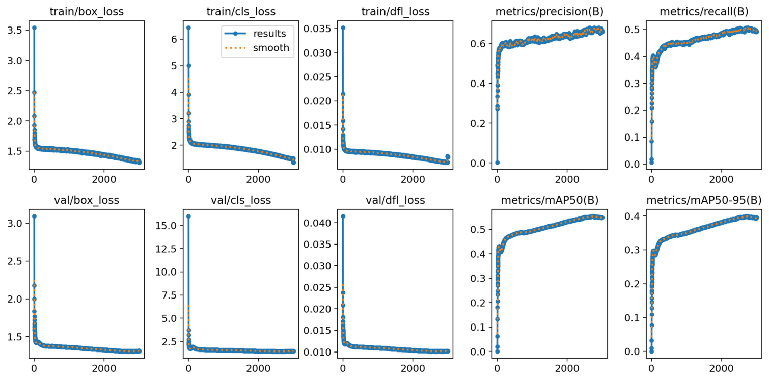
Training duration and convergence control. In preliminary experiments, we observed that YOLO26n trained from scratch may require extended training to reach peak validation mAP@0.50:0.95, with continued gains beyond typical short schedules. To reduce the risk of comparing under-trained variants, we set a maximum of 3000 epochs and enable early stopping with patience = 300, terminating training if validation mAP@0.50:0.95 fails to improve for 300 epochs. The best checkpoint is selected according to validation mAP@0.50:0.95 rather than training-set performance. This validation-based stopping and checkpoint-selection procedure helps limit overfitting risk while allowing each configuration sufficient opportunity to converge. The same schedule, augmentation settings, optimizer configuration, weight decay, and early-stopping rule are applied uniformly across the baseline and all ablations. Representative training and validation loss curves for the default and best combined configurations are provided in Appendix C.

Configuration transparency and reproducibility. Unless stated otherwise, all runs use the same base training configuration (training arguments and values) provided in the paper’s Appendix A. This includes optimizer and learning-rate schedule settings, augmentation parameters, image size, batch size, and any other training-time options that materially affect outcomes. The latency benchmarking arguments used to obtain inference times for each ablation are also documented to enable direct replication and are described in Appendix B.

Implementation, licensing, and availability note. The experiments in this study use the official Ultralytics YOLO26 implementation as the reference implementation. This manuscript does not provide or claim to provide a license-free independent implementation of YOLO26. Reproduction, modification, redistribution, or deployment of YOLO26-based models is subject to the applicable Ultralytics licensing terms. Ultralytics YOLO code and trained models are distributed under the AGPL-3.0 license by default, and Ultralytics offers an Enterprise License for organizations that wish to embed Ultralytics YOLO code or models into proprietary commercial products without the obligations associated with AGPL-3.0. Readers should, therefore, consult the official Ultralytics license terms before using YOLO26 in proprietary or closed-source deployment settings.

Ablation design. We focus on ablations that reflect meaningful architectural and implementation choices commonly considered by practitioners, including activation functions, C3k2 variants, SPPF settings, and attention module configurations. Each ablation is evaluated against the current Ultralytics baseline module or configuration under identical training and evaluation conditions. We report absolute performance in terms of both accuracy and inference speed.

Fixed-recipe interpretation note. All ablations were conducted with a fixed COCO training recipe, fixed data configuration, fixed optimizer settings, fixed augmentation settings, fixed early-stopping protocol, and fixed TensorRT benchmarking pipeline. This design supports controlled architectural attribution by ensuring that the observed differences are primarily associated with the architectural or configuration change under study. However, the results are conditional on this shared protocol. Different operators, activation functions, or architectural variants may require different hyperparameters to reach their individually optimal performance; for example, replacing SiLU with ReLU or Leaky ReLU may benefit from different learning rates, weight decay, warmup behavior, augmentation strength, or regularization settings. Therefore, the ablation results should be interpreted as controlled one-factor-at-a-time comparisons under a fixed recipe, rather than as evidence that each variant has reached its individually optimized performance or as a full neural architecture search with per-candidate hyperparameter tuning.

Outputs. The combined outcome of this methodology is (i) an interpretable, block-level explanation of YOLO26n and (ii) an evidence-backed set of ablation results that highlight which modules drive improvements and which offer limited benefit relative to their cost, guiding future architectural iterations and practical deployment decisions.

4. Network Architecture Overview

The YOLO26 model is organized into a sequence of stages and blocks that transform an input image through a hierarchical pipeline, ultimately producing multi-scale feature representations for detection.

The backbone initiates feature extraction. Early convolutional layers downsample the input, reducing spatial resolution while capturing low-level patterns such as edges and textures. These are followed by repeated C3k2 modules, which refine features efficiently by capturing local context and progressively strengthening representation capacity. As depth increases, shallow layers retain fine-grained spatial details, while deeper layers generate more abstract, high-level semantic features. This process yields feature maps at multiple scales (e.g., P3, P4, and P5), supporting detection of objects with varying sizes.

The SPPF module then aggregates information across multiple receptive-field scales, enriching the feature representation with broader contextual cues. Following this, the C2PSA module combines convolutional processing with position-sensitive attention to capture both local detail and longer-range dependencies while preserving spatial structure. This enhances the discriminative power of features at the backbone–neck interface and improves overall detection performance.

The neck further refines extracted features through multi-stage fusion. Upsampling operations increase spatial resolution, after which concatenation layers merge these features with corresponding features from earlier stages. C3k2 modules, together with upsampling and concatenation layers, combine low- and high-level features along channels, progressively upsampling or downsampling fused features to integrate information across layers [25,26,27]. Additional C3k2 modules then process the fused representations to enhance feature consistency and predictive performance across scales.

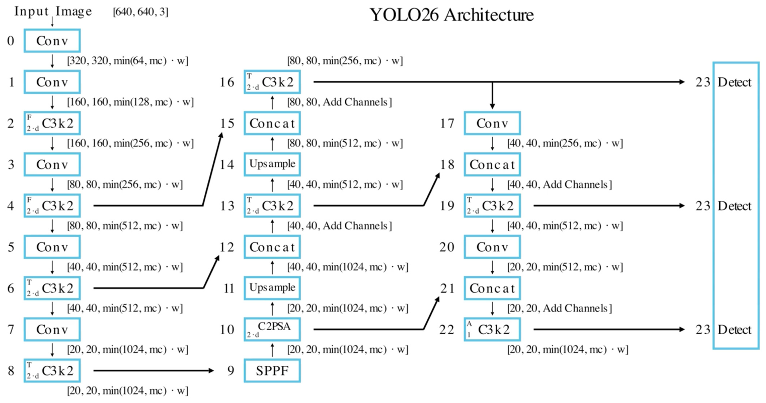
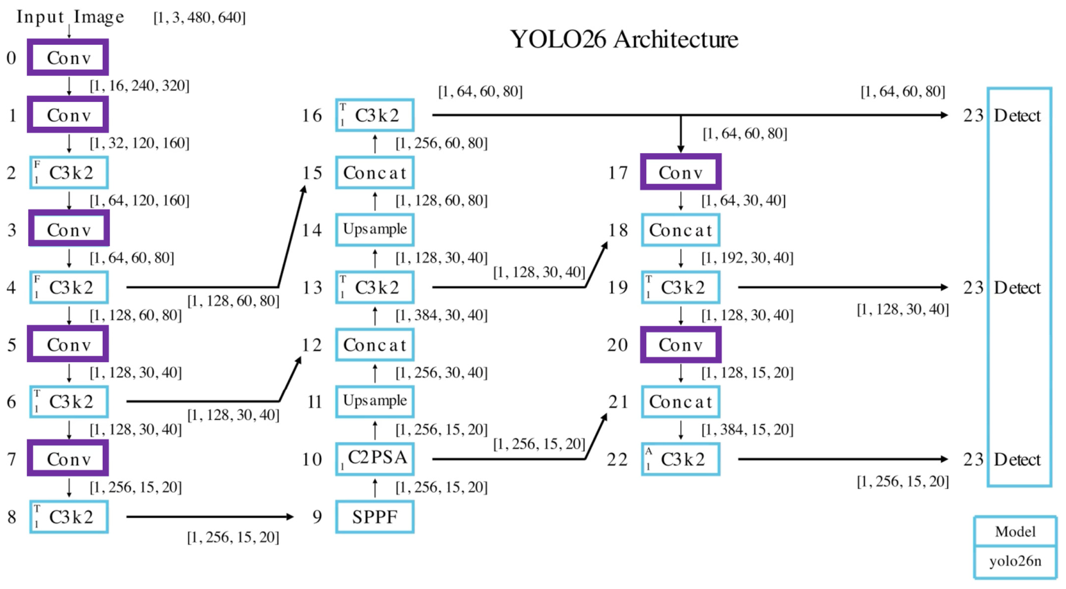
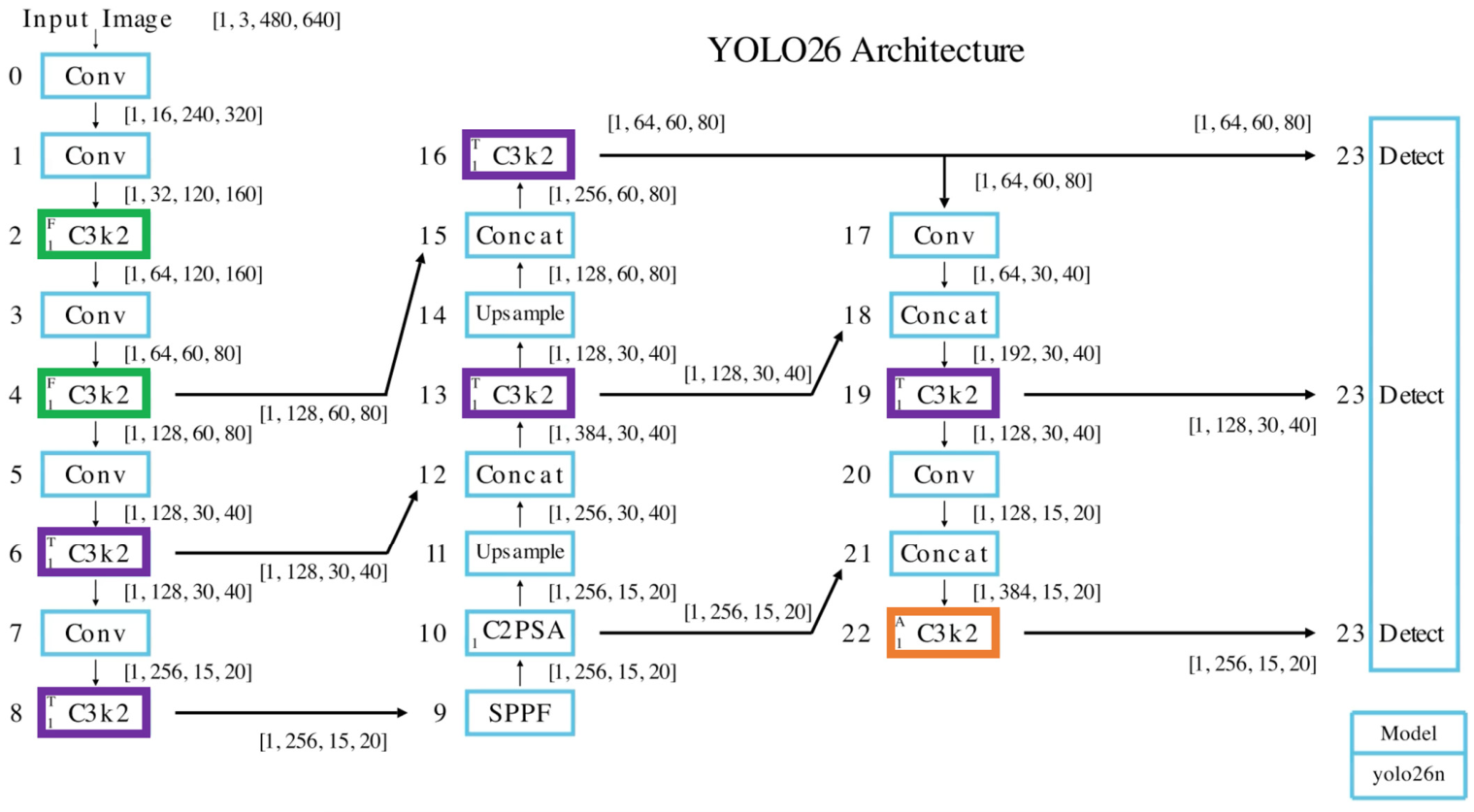
The overall architecture in Figure 1 is consistent across all YOLO26 variants: Nano, Small, Medium, Large, and Extra Large. The exact tensor dimensions at each stage are determined by two scaling parameters: w (width multiplier) and mc (maximum number of channels).

Additionally, the number of blocks in the C3k2 and C2PSA modules depends on the result of multiplying 2 by another parameter: d (depth multiplier).

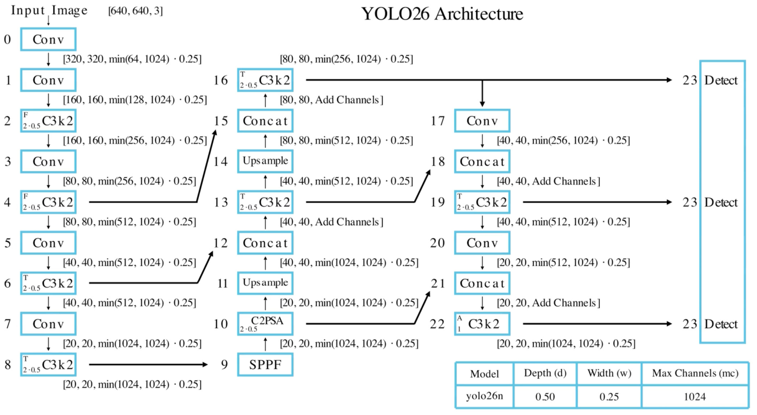
For example, in the nano configuration, the scaling parameters are set to a d or depth of 0.5, a w or width of 0.25, and an mc or maximum number of channels of 1024, as shown in Figure 2.

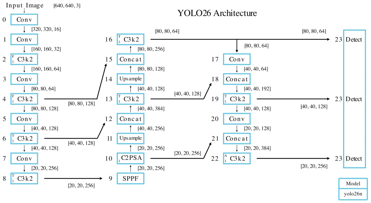
Substituting these values into the architecture formula yields the corresponding number of block repetitions and the tensor shapes at each stage, as shown in Figure 3.

We also explicitly note the shapes for the cross-stage tensor to further enhance clarity, as shown in Figure 4.

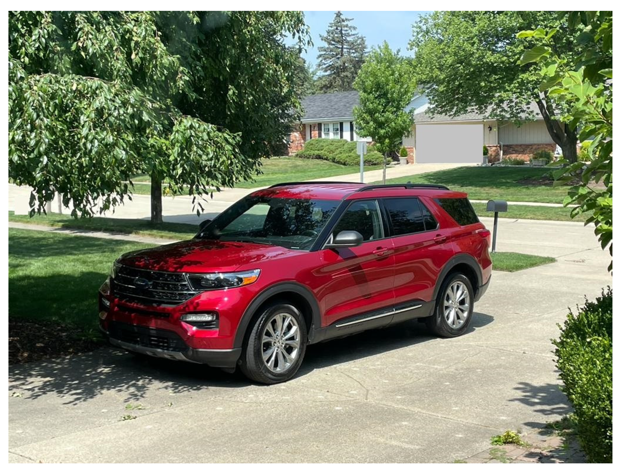
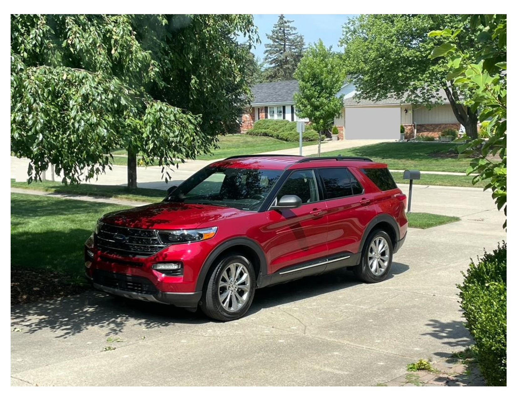
To illustrate how tensor shapes evolve through the network for a concrete input, we consider the example image shown in Figure 5, with original dimensions 768 × 1024 (height × width). Tensor shapes throughout the network depend on the spatial resolution of the input. Therefore, feature-map heights and widths vary with the input height and width and will differ for other input resolutions.

The network input is not required to be square (e.g., 640 × 640). In our preprocessing pipeline, images are resized while preserving aspect ratio such that the longer side is 640 pixels. The shorter side is then adjusted to be divisible by the network’s largest stride (32) to ensure that all downsampling stages produce integer-valued feature-map sizes. If necessary, letterboxing pads the image to the nearest multiple of 32.

Using this procedure, the example image in Figure 5 is resized (and, if necessary, letterboxed) to produce the network input of 480 × 640 × 3, shown in Figure 6.

The corresponding tensor shapes throughout the network (including intermediate cross-stage tensors) are reported in Figure 7. For consistency with PyTorch conventions, all tensor shapes are expressed as [batch, channels, height, width].

This notation and these dimensions are used throughout the paper as we examine individual modules and their internal steps.

5. Convolutional Block (Conv)

5.1. Objective

Convolutional layers are the backbone of neural networks for object detection, playing a vital role in the following:

• Feature extraction: By applying filters (kernels) to input data, they learn spatial hierarchies of patterns, such as edges, textures, shapes, and objects.
• Hierarchical learning: Stacking multiple layers allows for capturing increasingly abstract and complex features, from low-level edges in early layers to high-level representations in deeper layers.
• Progressive downsampling: These layers reduce the spatial dimensions of the input image (e.g., P1 → P2 → P3) while increasing channel depth. This process enables efficient feature compression, reducing computational cost while preserving critical information. By maintaining spatial relationships, the network retains the structural arrangement of the data and preserves meaningful features.
• Parameter sharing: Convolutional filters are reused across the input, reducing the number of learnable parameters and enabling translational invariance. Common variants include standard convolution (3 × 3), pointwise convolution (1 × 1), and depthwise convolution (DWConv) [28].

5.2. Flow

Each convolutional block consists of three sequential operations:

• Convolution: Applies a learned kernel (technically implemented as cross-correlation) to extract local spatial features.
• Batch normalization (BN) [29]: Normalizes intermediate activations to stabilize training and accelerate convergence.
• Activation: Introduces nonlinearity, enabling the network to model complex patterns. YOLO26 uses SiLU (also known as Swish) [30] as the default activation, which provides a smooth, nonlinear transformation. With sufficient SiLU neurons, the network can approximate complex functions with high fidelity.

During inference warmup, convolution and BN layers are typically fused. Because BN parameters are frozen after training, their scaling and shifting can be absorbed into the preceding convolution, producing a single convolutional layer with updated weights and biases. This pre-fusion step reduces computational overhead without altering the network’s behavior.

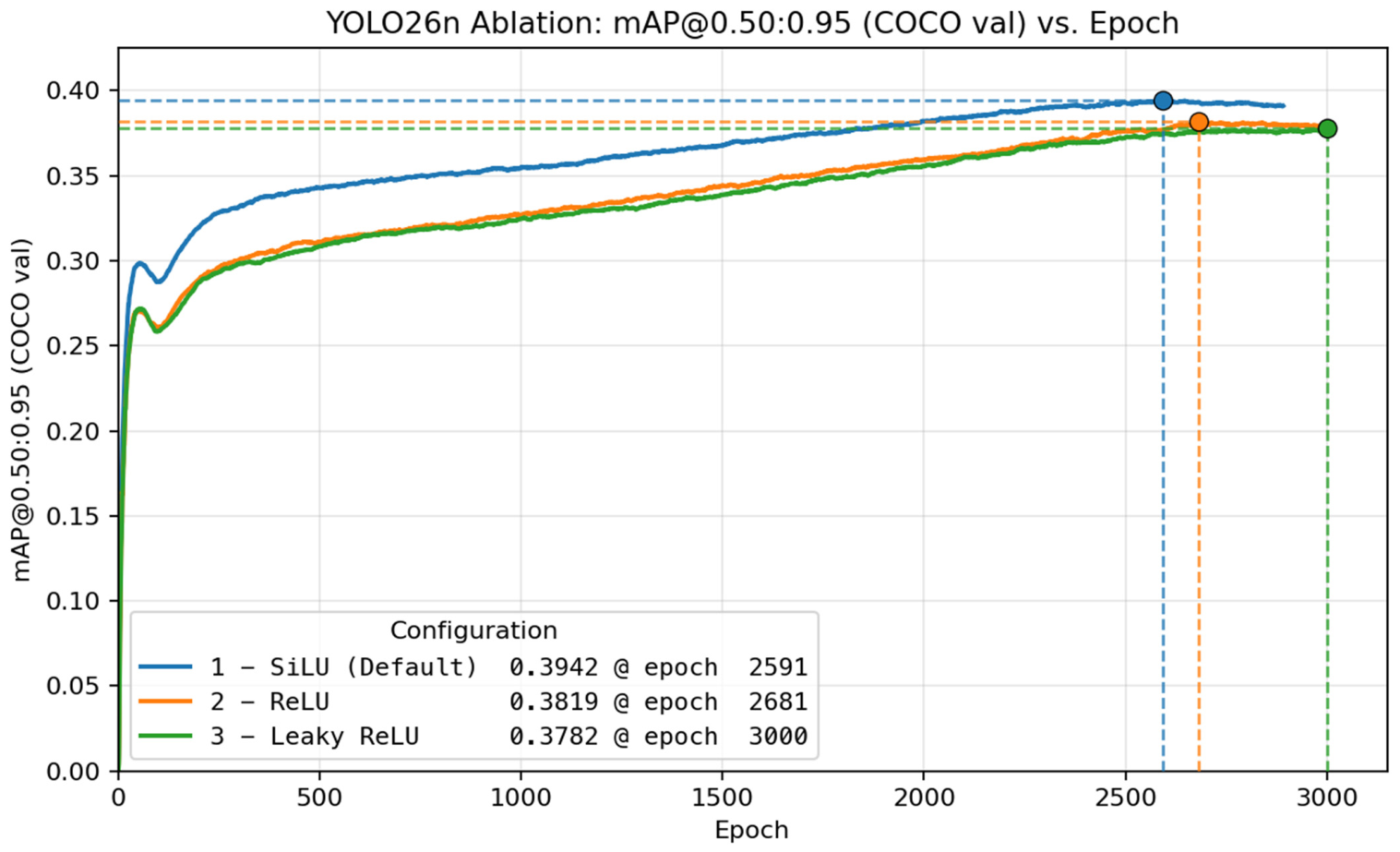
To analyze the effect of the activation function, we train three YOLO26n variants from scratch for up to 3000 epochs on the COCO dataset, differing only in their activation functions: (1) all SiLU, (2) all ReLU, and (3) all Leaky ReLU. As shown in Figure 8, the SiLU variant consistently achieves the highest mAP@0.50:0.95 across the entire training run, and training terminates early at epoch 2591 because no further improvement is observed.

Benchmarking these three activation variants on TensorRT 10 (FP16) with an H100 GPU (

Table 1. Activation function ablation results for YOLO26n. Bold values indicate the best result in each metric column.

Architecture	Parameters	GFLOPs	mAP@0.50:0.95	Latency (ms)
1—SiLU (Default)	2,572,280	6.1	0.3933 ± 0.00004	0.99 ± 0.04
2—ReLU	2,572,280	6.1	0.3808 ± 0.00010	0.93 ± 0.03
3—Leaky ReLU	2,572,280	6.1	0.3761 ± 0.00009	1.02 ± 0.03

) confirms a clear accuracy–latency trade-off. The default configuration (1, all SiLU) achieves the highest mAP@0.50:0.95 (0.3933) with a TensorRT FP16 latency of 0.99 ms. Switching to ReLU (2) produces the lowest latency (0.93 ms) but reduces accuracy to 0.3808 mAP@0.50:0.95. Using Leaky ReLU (3) provides no benefit: it yields the lowest accuracy (0.3761) while remaining slower than ReLU at 1.02 ms. Therefore, between ReLU and Leaky ReLU, ReLU is preferable on both accuracy and latency.

Ultralytics adopts SiLU because the accuracy improvement over ReLU is substantial (0.3933 vs. 0.3808 mAP@0.50:0.95), and this gain can justify the modest latency increase for applications where detection quality is prioritized. In this sense, SiLU represents the best overall accuracy-focused choice among the tested activations, while ReLU is the best speed-focused alternative.

6. Feature Refinement Module (C3k2 with Argument False)

6.1. Objective

The C3k2 (F) module is a lightweight feature refinement block designed to efficiently enrich and transform features within the YOLO26 architecture. Standard deep networks often suffer from computational redundancy, where the same information is processed multiple times across layers. The Cross-Stage Partial (CSPNet) approach [31] mitigates this by splitting the feature map into two parts:

• Refinement path: one part passes through a compact bottleneck with residual connections [32] to extract refined features.
• Shortcut path: the other bypasses the bottleneck entirely.

The two paths are then recombined through concatenation, followed by a projection into a richer, more discriminative feature space. This design improves representational capacity while preserving computational efficiency. Inside the C3k2 (F) module, the bottleneck block excels in several key areas:

• Compression phase (squeezing features): The first convolution in the bottleneck block reduces the input channels. This dimensionality reduction focuses on distilling the most critical information while discarding less important features.
• Processing in the bottleneck: The reduced feature set undergoes transformations (convolutions and activations) to refine patterns efficiently. This step emphasizes core patterns while conserving computational resources.
• Expansion phase (rebuilding features): The final convolution expands the channels back to ensure the network retains capacity for complex pattern modeling. This combines the critical features from compression with the structural richness needed for downstream tasks.
• Promoting a compact and informative representation: By alternating between high- and low-dimensional spaces, the bottleneck prioritizes relevant features, retaining only the most useful information.
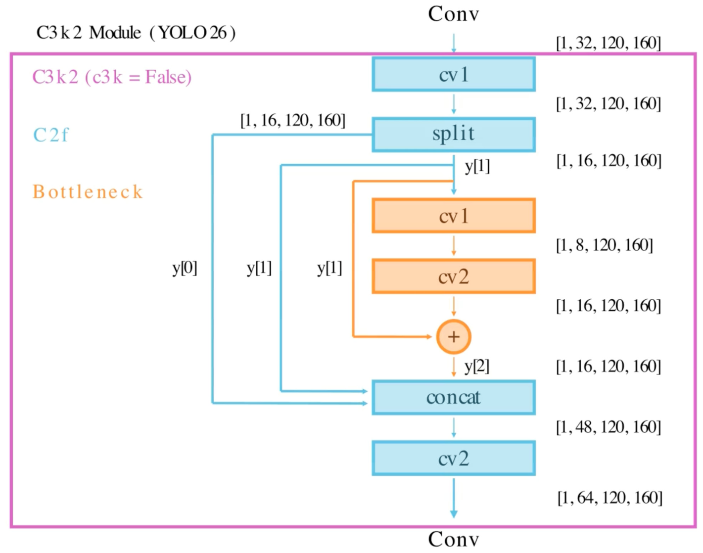
• Scalability: In YOLO26, C3k2(F) scales its internal depth with model size: nano/small/medium use one bottleneck, while large/extra-large use two bottlenecks in series between split and concat. Figure 9 illustrates the C3k2(F) feature-refinement module with c3k = False.

The C3k2 module represents YOLO26’s evolution of the C2f module, first introduced in YOLOv8 by Ultralytics [8]. The C2f structure subsequently became a key building block in modern YOLO architectures, such as YOLOv10 [10] and YOLO11 [11], typically incorporating a default bottleneck module. Originally introduced in YOLOv3 [3], the bottleneck has remained a core component of increasingly sophisticated modules across successive YOLO versions. By leveraging the C3k2 module, YOLO26 achieves high precision while using fewer parameters than its predecessors [17], making it computationally efficient without sacrificing accuracy.

6.2. Flow

The operations within the C3k2 (F) module are as follows:

• Initial convolution (cv1): A 1 × 1 convolution is applied to the input tensor, preserving spatial resolution while transforming features and mixing channels.
• Split: The input tensor is divided along the channel dimension into two groups (32 channels → 16 + 16). One half (y[0]) is preserved for an identity/skip connection, while the other half (y[1]) is passed through the bottleneck for transformation.
• Bottleneck: The bottleneck processes y[1] via two consecutive 3 × 3 convolutions. The first reduces channels (16 → 8), compressing information and enabling learning in a reduced space. The second restores channels to the original number (8 → 16), expanding the feature representation while incorporating local spatial context. This encourages the network to capture structured patterns (curves, corners, and textures) that are critical for object boundaries and class distinctions.
• Concatenation: The outputs from the split step and the bottleneck result are concatenated along the channel axis (y = [y[0], y[1], bottleneck’s output]). This operation merges raw and transformed features, creating a multi-view representation that enhances the network’s ability to detect diverse patterns.

Because y[0] and y[1] are passed through unchanged, the network can learn the optimal balance between retaining original input features and incorporating the bottleneck-processed features. This design also facilitates better gradient flow during training.

• Final convolution (cv2): A 1 × 1 convolution is applied to the concatenated tensor to learn inter-channel relationships and project the features to the desired number of channels (48 → 64), enriching the feature space.

7. Feature Refinement Module (C3k2 with Argument True)

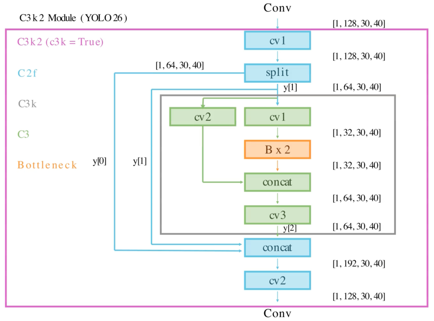
All C3k2 (T) modules are highlighted in green in the architecture diagram below.

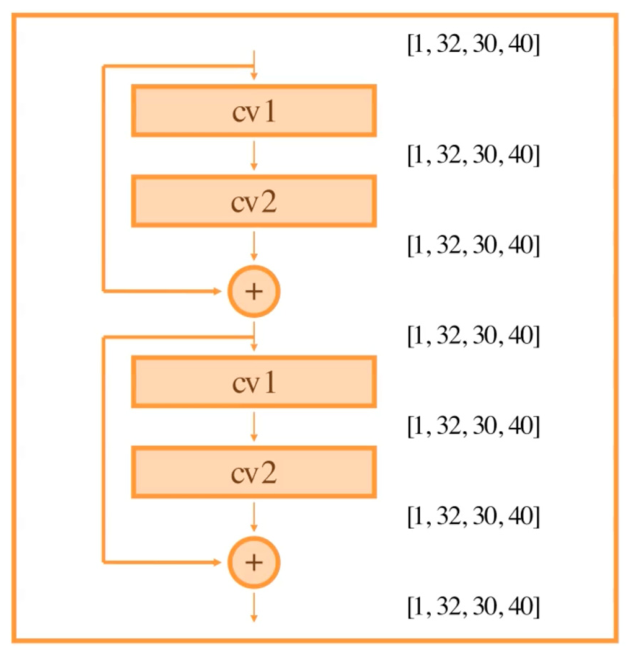
The double-bottleneck from Figure 10 is further expanded below in Figure 11 for more clarity.

7.1. Objective

The C3k2 (T) block is the heavier variant of the C3k2 module, designed to deepen feature refinement via C3k modules with nested bottlenecks. By applying multi-stage transformations within each partition of the input, the approach increases the richness and diversity of feature representations. This module extends the C2f design with a customizable double-bottleneck structure, allowing more sophisticated hierarchical feature processing while maintaining computational efficiency.

Inside the C3k2 (T) module, the C3k block excels in several key areas:

• Hierarchical compression (squeezing features): The initial convolutions reduce the input channels and partition features into smaller, more manageable subsets. This hierarchical compression retains the most critical information, optimizing for both efficiency and diversity of feature representation.
• Multi-stage processing within C3k: Each subset undergoes further refinement through a series of nested bottleneck blocks. These blocks sequentially transform the compressed features to emphasize core patterns while discarding redundancies.
• Final expansion and aggregation: The outputs of the bottleneck blocks are recombined and expanded through concatenation and the final convolution. This phase balances dimensionality and feature richness, ensuring the network is prepared for subsequent stages.
• Promoting feature diversity and refinement: By incorporating multiple convolutional paths and iterative processing, the C3k block enhances the diversity of extracted patterns. This design ensures that both fine-grained and broader structural features are effectively captured.
• Scalability: In YOLO26, C3k2(T) scales its internal depth with model size: nano/small/medium use one C3k, while large/extra-large use two C3k blocks in series between split and concat (each C3k contains two bottleneck blocks).

C3k2(T) inherits from the C2f block (like C3k2(F)) but introduces hierarchical feature refinement via the C3k sub-block. Instead of the standard bottleneck used in C3k2(F), it employs a C3k module, a C3-style block with three convolutions and an internal double-bottleneck design, enabling deeper feature refinement within each split partition.

7.2. Flow

The operations within the C3k2 (T) module are as follows:

• Initial convolution (cv1): 1 × 1 convolution projects the input tensor for partitioned processing.
• Partitioning: The tensor is split along the channel dimension into two partitions: the identity path and the processed path.
• C3k path (c3k = True): The processed partition is passed through a C3k block with an internal double-bottleneck design that uses 3 × 3 kernels to enhance spatial feature extraction and refinement.
• Concatenation: Merge input paths (y[0] and y[1]) and the C3k output along channels.
• Final convolution (cv2): 1 × 1 convolution projects the concatenated tensor to the desired number of channels for downstream modules.

8. C3k2 Module Variants: Architecture Placement and Design Trade-Offs

As we have seen, the C3k2 module in YOLO26 supports two configurations via the c3k flag. The lightweight path (c3k = False) contains a single bottleneck block, providing low computational cost and capturing shallow residual context, making it suitable for early-stage processing with large feature maps. The heavier path (c3k = True) incorporates a C3 module with nested bottlenecks, enabling deeper, nonlinear transformations and richer feature representations for later stages. In short, c3k = False prioritizes efficiency, while c3k = True emphasizes representational capacity.

As shown in Figure 12, the placement of C3k2 variants reflects a deliberate, stage-wise allocation of computational resources, guided by feature map size, computational cost, and semantic requirements.

• Early backbone stages (Stages 2 and 4 in green): c3k = False is used since feature maps are large (high spatial resolution). Lightweight bottlenecks capture low-level features such as edges and textures while keeping computation low.
• Deeper backbone stages (Stages 6 and 8 in purple): c3k = True is employed as feature maps become smaller (lower spatial resolution, higher channel depth). Heavier processing enables deeper, nonlinear transformations that capture object parts and semantic patterns.
• Neck layers (Fusion Stage 13 and Final Stages 16 (P3) and 19 (P4)): The fusion stage and the final P3 and P4 stages use c3k = True to efficiently integrate multi-scale features.

The Final Stage 22 in orange (P5) employs a special module newly introduced in YOLO26. We discuss this module later, after the C2PSA module, because it shares similar attention components.

The alternating use of c3k = False and c3k = True balances efficiency and expressiveness: using only c3k = False favors speed but limits high-level feature extraction, reducing accuracy for complex objects, whereas using only c3k = True enhances accuracy but significantly increases inference latency in early stages with large feature maps.

YOLO26 balances these considerations by employing lightweight blocks in early layers for efficiency, heavier blocks in deeper layers for richer feature extraction, and in the neck for strong semantic reasoning. This placement aligns with general CNN design principles, prioritizing efficiency when feature maps are large and capacity when spatial resolution is low, optimizing the network’s speed-accuracy trade-off.

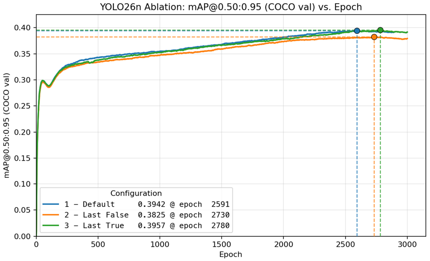
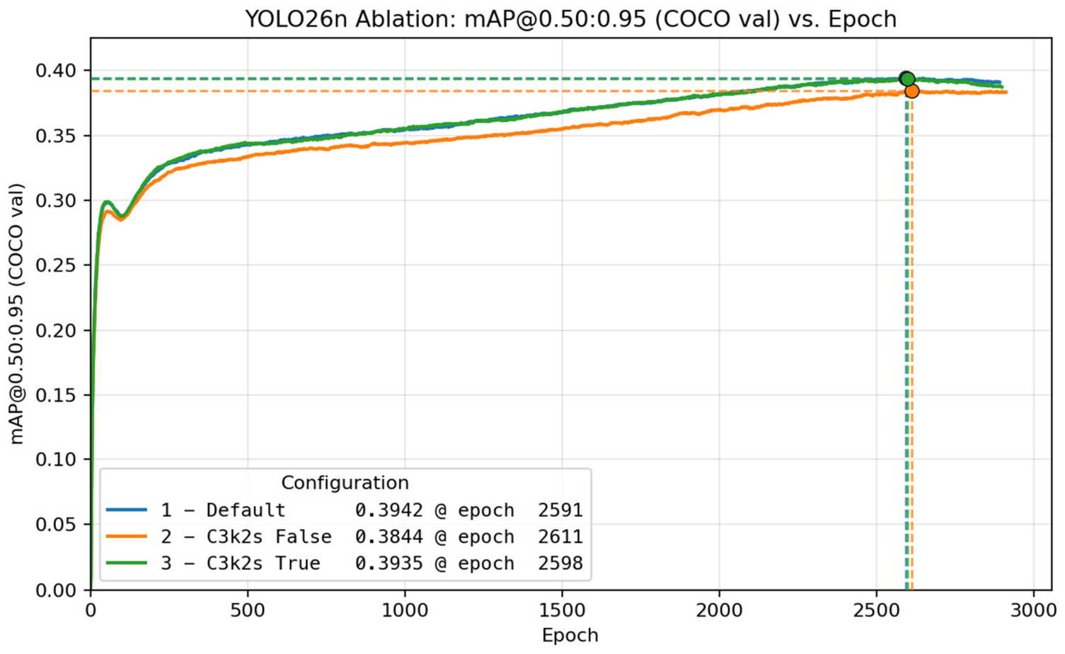
To justify the deliberate selection of C3k2 configurations, we train three YOLO26n variants from scratch for up to 3000 epochs on the COCO dataset: (1) the original architecture, which employs a mixture of c3k = False and c3k = True settings; (2) a variant in which all C3k2 modules use c3k = False; and (3) a variant in which all C3k2 modules use c3k = True. Stage 22 is kept unmodified in these experiments, as its design is examined separately later in the paper.

Benchmarking on TensorRT 10 (FP16) with an H100 GPU (

Table 2. C3k2 configuration ablation results for YOLO26n. Bold values indicate the best result in each metric column.

Architecture	Parameters	GFLOPs	mAP@0.50:0.95	Latency (ms)
1—C3k2s (Default)	2,572,280	6.1	0.3933 ± 0.00004	0.99 ± 0.04
2—C3k2s False	2,511,128	6.0	0.3813 ± 0.00004	0.86 ± 0.03
3—C3k2s True	2,575,080	6.2	0.3930 ± 0.00015	1.11 ± 0.04

) confirms the accuracy–latency trade-off introduced by the C3k2 configuration. Model 3 (all C3k2 modules set to True) achieves very similar accuracy to the baseline (0.3930 vs. 0.3933 mAP@0.50:0.95), but incurs the highest latency (1.11 ms), making it a net regression in efficiency. Conversely, Model 2 (all C3k2 modules set to False) is the fastest configuration (0.86 ms), but suffers from an accuracy drop to 0.3813 mAP@0.50:0.95.

Overall, Model 1 (the default YOLO26n mix of C3k2 False and True) provides the best accuracy–speed balance. It preserves the highest accuracy while avoiding the additional runtime cost observed when enabling C3k2 True throughout the network. These results, also illustrated by the validation mAP@0.50:0.95 curves over training epochs in Figure 13, indicate that setting all C3k2 modules to True provides no measurable accuracy benefit yet increases latency, whereas retaining the mixed design—using the more expensive configuration only where it is most impactful—yields the most practical trade-off.

9. SPPF Module (Spatial Pyramid Pooling Fast)

9.1. Objective

The SPPF block enriches deep features with multi-scale spatial context. Its primary goals are:

• Multi-scale feature aggregation: Applies three max-pooling operations (kernel size = 5) to capture spatial information at multiple scales, combining fine details and broad context.
• Feature fusion: Concatenates outputs from pooling operations to create a rich, multi-scale feature map, enhancing the network’s ability to detect objects of varying sizes.
• Efficient downsampling: Preserves spatial relationships while reducing resolution, ensuring compact and meaningful feature representation.
• Optimized design: Streamlines traditional SPP, reducing computations while maintaining scalability for real-time applications.

SPPF was introduced in YOLOv5 as a faster alternative to the original SPP module (used in YOLOv5 first releases). The SPPF module has since been used in subsequent YOLO architectures, including YOLOv6 [6], YOLOv8 [8], YOLOv10 [10], and YOLO11 [11].

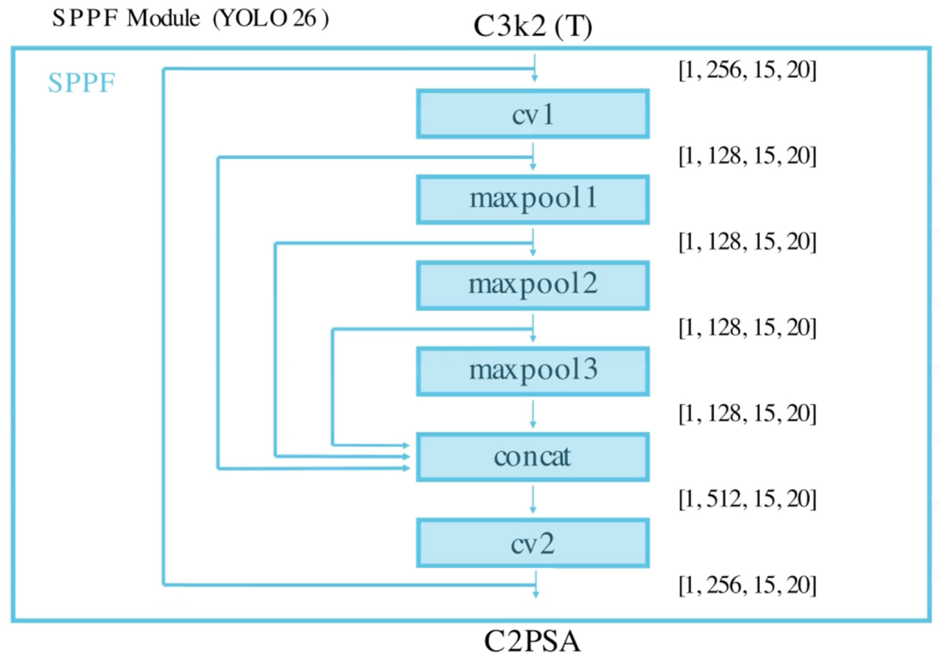
YOLO26 adopted the SPPF as the standard pooling module due to its combination of accuracy and efficiency but added the residual connection from the input to the output, not used in previous versions. They also hardcoded the two convolutions (cv1 and cv2) to not have activation (act = False), unlike previous versions, which did have it (act = True). Figure 14 illustrates the YOLO26 SPPF module, including the repeated max-pooling operations, feature concatenation, projection layer, and residual connection.

9.2. Flow

• Initial convolution (cv1): A 1 × 1 convolution reduces the number of channels to prepare the input for multi-scale pooling.
• Multi-scale max-pooling: Three parallel max-pooling operations (kernel size = 5) capture features at different receptive fields while preserving spatial relationships.
• Concatenation: Outputs of all pooling operations and the initial convolution are concatenated along the channel dimension, producing a multi-scale feature map.
• Final convolution (cv2): A 1 × 1 convolution projects the concatenated feature map back to the desired number of channels, creating a compact, enriched representation for downstream processing.

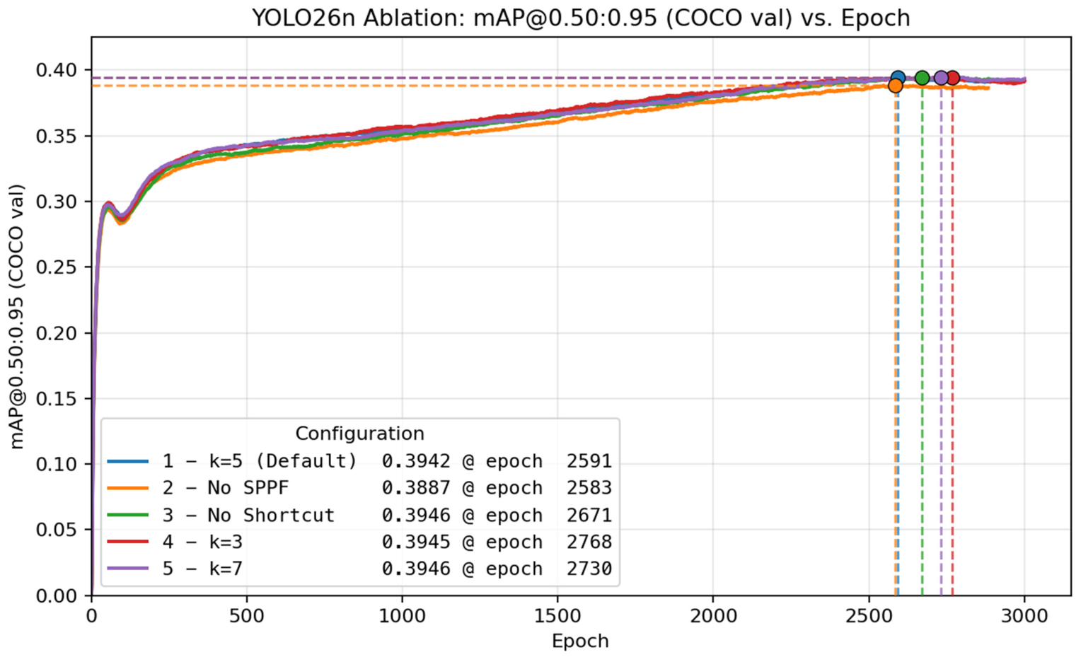
To analyze the contribution of the SPPF module and evaluate its main design choices, we train five YOLO26n variants from scratch for 3000 epochs on the COCO dataset. Among these, three differ only in the max-pooling kernel size used in the SPPF module, one omits the SPPF module entirely, and one disables the newly introduced residual connection. Figure 15 shows the five configurations: (1) default kernel_size = 5, (2) no SPPF module, (3) no shortcut, (4) kernel_size = 3, and (5) kernel_size = 7.

Benchmarking the five SPPF configurations with TensorRT 10 (FP16) on an H100 GPU (

Table 3. SPPF module ablation results for YOLO26n. Bold values indicate the best result in each metric column.

Architecture	Parameters	GFLOPs	mAP@0.50:0.95	Latency (ms)
1—k = 5 (Default)	2,572,280	6.1	0.3933 ± 0.00004	0.99 ± 0.04
2—No SPPF	2,407,672	6.0	0.3866 ± 0.00007	0.96 ± 0.01
3—No Shortcut	2,572,280	6.1	0.3941 ± 0.00013	1.01 ± 0.03
4—k = 3	2,572,280	6.1	0.3922 ± 0.00004	1.00 ± 0.02
5—k = 7	2,572,280	6.1	0.3935 ± 0.00007	0.98 ± 0.01

) highlights a nuanced accuracy–latency trade-off. The baseline configuration (Model 1, SPPF with k = 5) delivers strong overall performance, achieving 0.3933 mAP@0.50:0.95 with a latency of 0.99 ms. Removing the SPPF module entirely (Model 2) yields the lowest latency (0.96 ms), confirming that eliminating this block improves inference speed; however, it also produces the lowest accuracy (0.3866 mAP@0.50:0.95), indicating that the loss of multi-scale feature aggregation degrades detection quality.

Among the tested variants, Model 3 (no shortcut) achieves the highest mAP@0.50:0.95 (0.3941) but also incurs the highest latency (1.01 ms). This makes it the most accuracy-focused option, although the accuracy gain over the baseline is small and comes at a modest runtime cost. Model 5 (k = 7) provides the most favorable standalone accuracy–latency trade-off among the SPPF kernel-size variants: it attains 0.3935 mAP@0.50:0.95 numerically but only marginally exceeds the baseline value of 0.3933, while also reducing latency to 0.98 ms. By contrast, Model 4 (k = 3) slightly reduces accuracy (0.3922 mAP@0.50:0.95) while also increasing latency (1.00 ms), offering no clear practical advantage over the baseline.

Overall, these standalone SPPF results suggest that removing SPPF is beneficial only when minimizing latency is the primary objective, whereas increasing the kernel size to k = 7 gives the best observed accuracy–latency balance within this isolated SPPF ablation. If maximum accuracy is prioritized above all else, the no shortcut variant is the strongest option.

It is important to note, however, that the standalone improvement of k = 7 over the default k = 5 is extremely small. Specifically, k = 7 improves mAP@0.50:0.95 from 0.3933 to 0.3935, corresponding to an absolute gain of only 0.0002. Therefore, this result should be interpreted as a marginal standalone improvement rather than definitive evidence that k = 7 is universally superior to k = 5. This distinction is important because the final combined-configuration experiments show that architectural changes are not necessarily additive. In the final best-combination study, the configuration using k = 5 achieves 0.3969 mAP@0.50:0.95, whereas the corresponding configuration using k = 7 achieves 0.3958. This indicates a non-additive interaction, or negative transfer, between the larger SPPF receptive field and the larger C2PSA attention ratio of 0.75. Increasing the SPPF kernel size expands local multi-scale pooling and increases the effective receptive field before the neck, while increasing the C2PSA attention ratio strengthens the attention branch’s ability to aggregate broader spatial context. When applied independently, each change may provide useful contextual information. When combined, however, the two mechanisms may become partially redundant or may overemphasize broad contextual aggregation in a nano-scale model with limited capacity. The larger SPPF kernel can introduce stronger spatial smoothing, while the larger attention ratio also emphasizes long-range dependencies. Together, these effects may reduce the balance between local detail and global context, which can be particularly harmful for small-object localization. For this reason, the final selected configuration uses k = 5, even though k = 7 is marginally better in the isolated SPPF ablation.

For the kernel-size variants, the parameter count and reported GFLOPs remain unchanged because changing k modifies only the MaxPool2d receptive field inside SPPF. The learnable operations in the block remain the same two 1 × 1 convolutions, and MaxPool2d introduces no trainable parameters. With fixed input/output channels and a fixed number of pooling iterations, the concatenated tensor passed to the second 1 × 1 convolution has the same channel dimension for k = 3, k = 5, and k = 7. Therefore, these variants have identical learnable model complexity and the same reported convolution-dominated GFLOPs, even though their measured TensorRT latencies can differ due to backend-specific pooling implementation, memory-access behavior, scheduling, fusion opportunities, and hardware utilization.

10. C2PSA Module (Cross-Stage Partial with Position-Sensitive Attention)

10.1. Objective

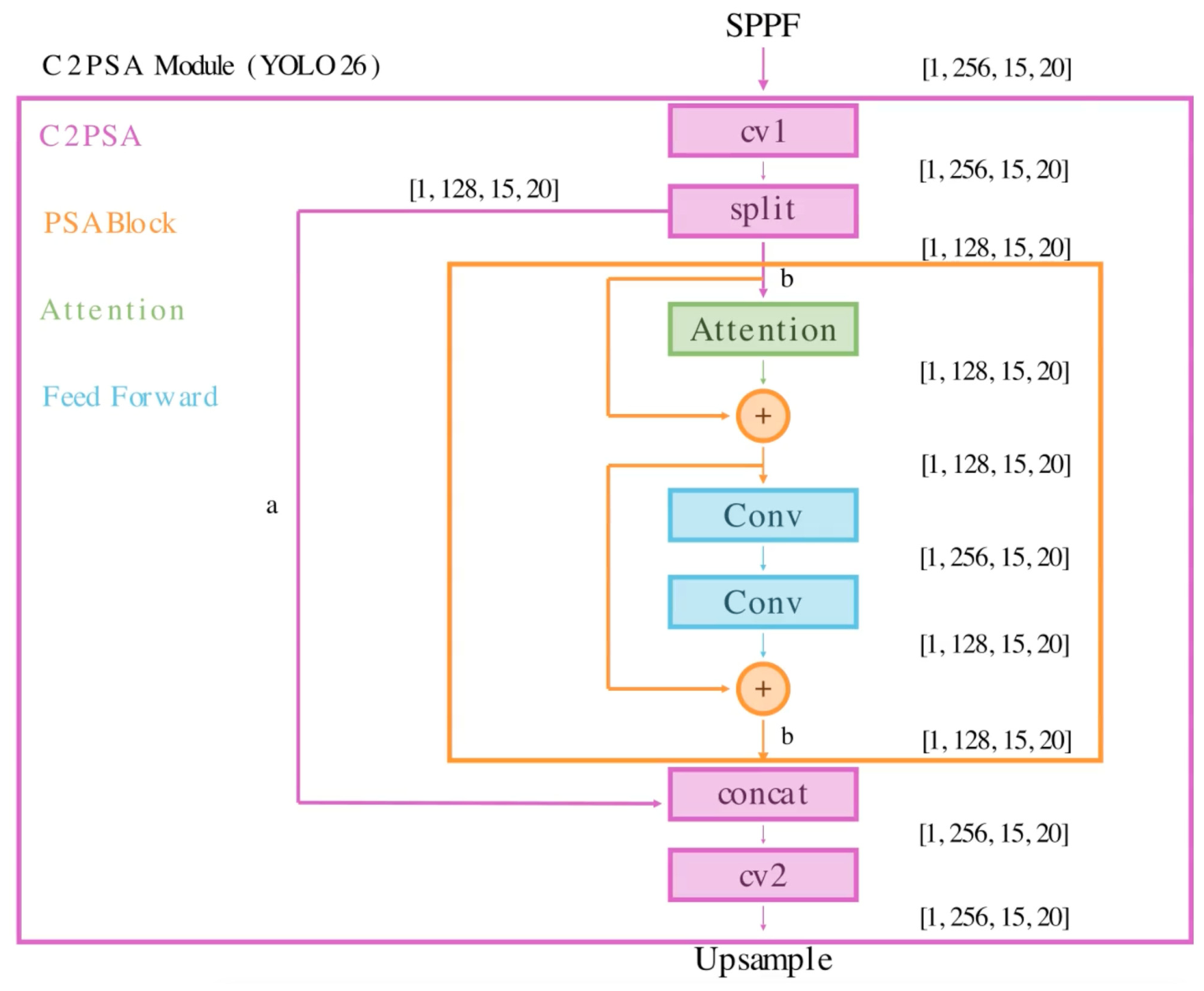
The C2PSA (Cross-Stage Partial with Position-Sensitive Attention) module is a key block in YOLO26, positioned after the SPPF and serving as the transition between the backbone and the neck. Its primary function is to enrich feature representations by combining convolutional processing with advanced attention mechanisms. Figure 16 shows the C2PSA module used at the backbone–neck interface of YOLO26n.

The C2PSA enhances feature extraction and processing through several complementary mechanisms:

• Dual-path processing: Input features are split into two pathways. One path undergoes direct convolutional processing to preserve local details, while the other applies attention-based transformations via PSABlock modules to capture long-range dependencies.
• Attention mechanisms: Each PSABlock leverages multi-head self-attention to model relationships between distant spatial locations, making the network more effective at handling complex and distributed object patterns.
• Spatial awareness: Position-sensitive encodings are incorporated to preserve relative spatial arrangements, strengthening localization accuracy.
• Feature refinement: Lightweight feed-forward layers within the PSABlock refine attended features, ensuring efficient propagation and richer semantic context.
• Feature fusion: Outputs from convolutional and attention pathways are merged, resulting in more expressive feature maps that balance local detail with global context.
• Scalability: Unlike YOLOv10 [10], where the PSA module was restricted to a single attention + feed-forward structure, YOLO26’s C2PSA allows multiple PSABlocks to be stacked. Smaller versions (nano, small, and medium) contain one PSABlock, while larger models (large and extra-large) contain two in sequence.

By integrating convolutional and attention-driven processing, the C2PSA module establishes attention as a central component in YOLO26, improving the discriminative power of the backbone–neck interface while preserving computational efficiency.

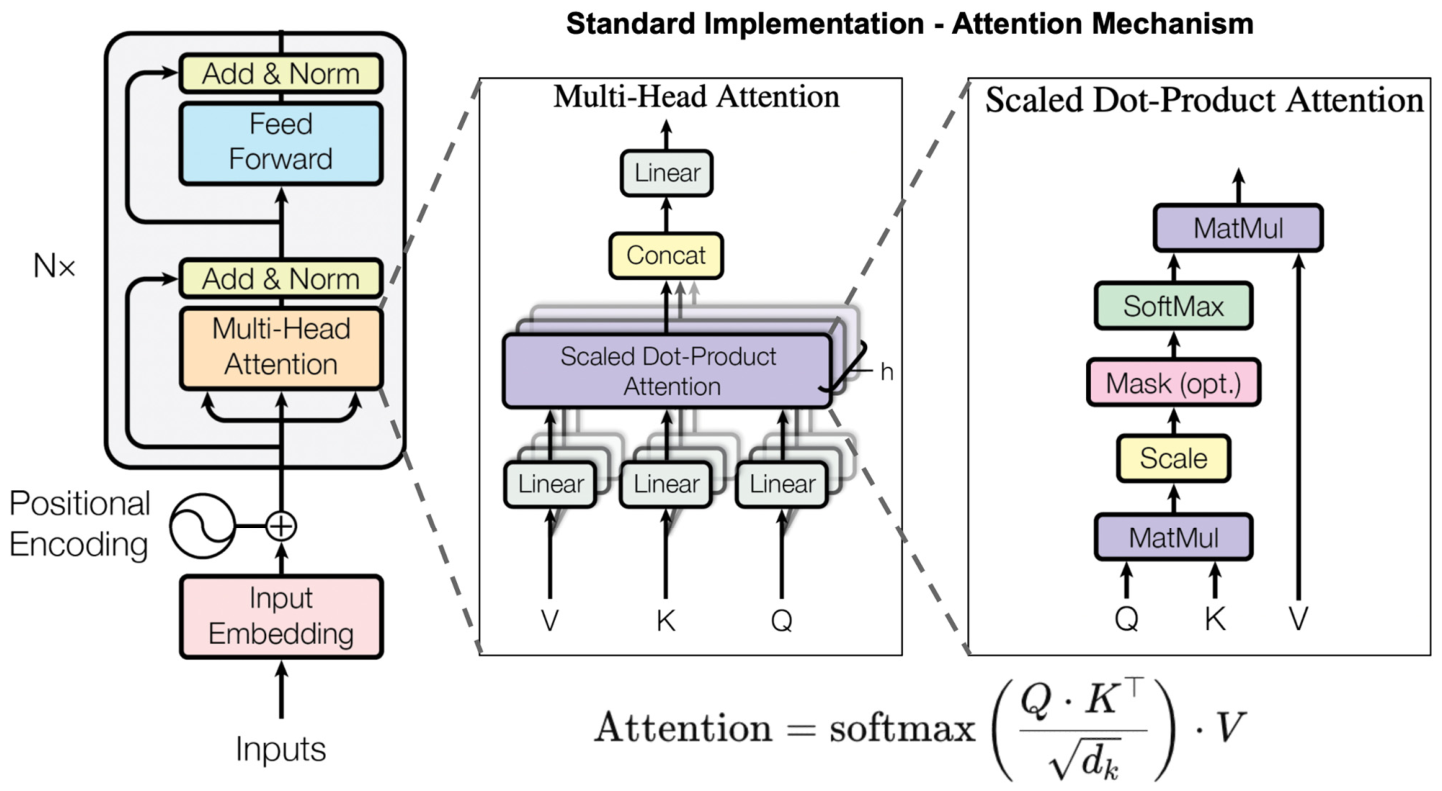
The standard attention mechanism, introduced in the original Transformer paper [33], forms the basis for many modern models. Figure 17 illustrates this mechanism.

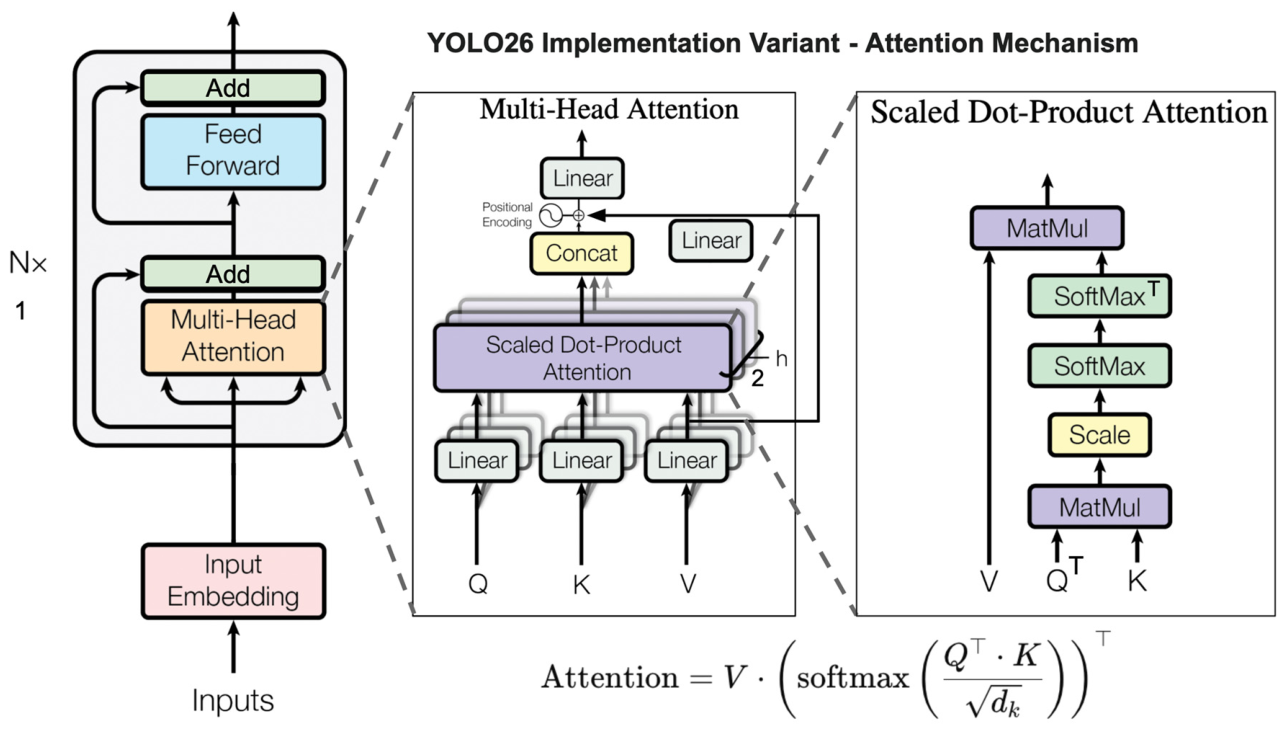
As seen in Figure 18, YOLO26 adopts a variant of this mechanism. Although mathematically similar to the standard method, this variation is optimized for vision tasks and requirements within the YOLO architecture, such as improving computational efficiency and simplifying implementation.

10.2. Flow

• Initial convolution (cv1): A 1 × 1 convolution preprocesses the input tensor, decoupling the module’s internal operations from preceding feature representations while maintaining spatial resolution.
• Split: The tensor is partitioned along the channel dimension into two branches: (a) a skip path that preserves identity features for later concatenation, and (b) a processed path that passes through the PSA block(s) for attention-based refinement.
• PSA block(s) for multi-head attention:

Queries, keys, and values are computed using a single 1 × 1 convolution for efficiency. This step applies a linear, activation-free projection that maps features into a new representation space while avoiding additional nonlinearity that may hinder optimization.

The channels are then split into multiple attention heads, allowing each head to learn different spatial relationships.

Scaled dot-product attention is computed to capture global similarity across spatial positions.

Softmax normalization is applied to produce interpretable attention weights.

A weighted sum of the value vectors is then generated, producing context-aware features enriched with global dependencies.

Positional encoding: A depthwise convolution [28] is applied to the value tensor to introduce local spatial awareness while preserving tensor dimensions. Let the input to the attention submodule be represented as B × C × H × W, where B is the batch size, C is the number of channels, and H and W are the spatial dimensions. The 1 × 1 QKV projection generates query, key, and value tensors, which are reshaped into multiple heads over N = H × W spatial positions. Although the query and key channel dimensions depend on the attention ratio, the value tensor retains the full per-head value dimension, so after concatenating the heads, it can be reshaped back to B × C × H × W.

The attention operation produces an attended-value tensor with shape B × C × H × W. In parallel, the value tensor is reshaped to B × C × H × W and passed through a stride-1 depthwise convolution with padding chosen to preserve H and W. Because the depthwise convolution uses one spatial filter per channel, it injects local positional bias without changing the channel count or spatial resolution. The resulting positional term, therefore, also has shape B × C × H × W. Since the attended-value tensor and the positional term have identical dimensions, they are combined by direct element-wise addition before the final projection convolution. No interpolation, spatial broadcasting, or channel remapping is required.

• Feed-Forward Network (FFN):

Applies a position-wise transformation to each spatial location independently, where 1 × 1 convolutions adjust channel representations without mixing information across neighboring pixels.

Uses an expand–compress design to enrich feature representations efficiently.

Incorporates skip connections to preserve original context and avoid over-smoothing.

• Concatenation and final convolution (cv2):

Merges the skip path (a) with the processed path (b) from the PSA block(s).

Final 1 × 1 convolution stabilizes the combined features and projects them into a compact representation suitable for downstream tasks.

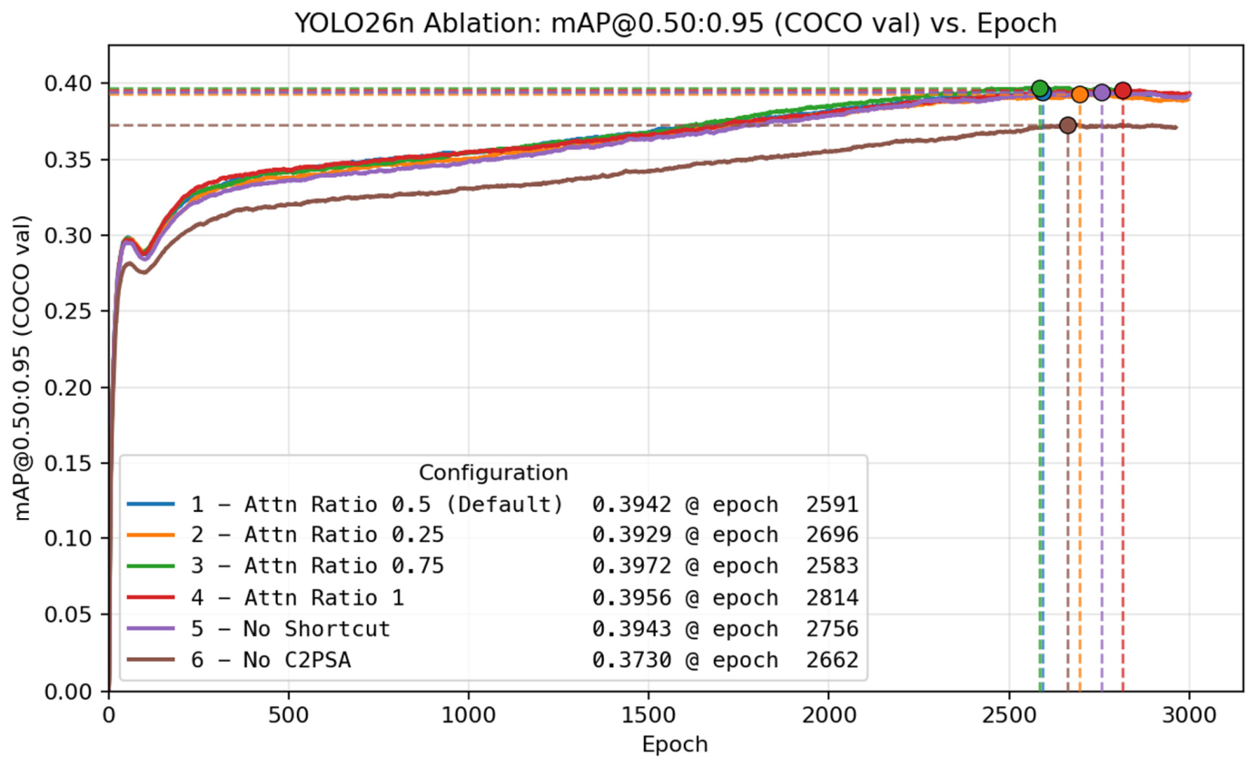
To analyze the contribution of the C2PSA module and evaluate its main design choices, we train six YOLO26n variants from scratch for 3000 epochs on the COCO dataset. The following Figure 19 presents the six configurations: (1) the standard YOLO26n model; (2) a variant with the attention ratio set to 0.25 instead of the default 0.5; (3) a variant with the attention ratio set to 0.75; (4) a variant with the attention ratio set to 1.0; (5) a variant in which the PSABlock shortcut connection is disabled; and (6) a variant in which the C2PSA module is removed entirely.

Benchmarking the six configurations on TensorRT 10 (FP16) with an H100 GPU (

Table 4. C2PSA attention-ratio and PSABlock shortcut ablation results for YOLO26n. Bold values indicate the best result in each metric column.

Architecture	Parameters	GFLOPs	mAP@0.50:0.95	Latency (ms)
1—Attn Ratio 0.5 (Default)	2,572,280	6.1	0.3933 ± 0.00004	0.99 ± 0.04
2—Attn Ratio 0.25	2,563,960	6.1	0.3909 ± 0.00000	0.99 ± 0.02
3—Attn Ratio 0.75	2,580,600	6.1	0.3961 ± 0.00004	0.99 ± 0.02
4—Attn Ratio 1	2,588,920	6.1	0.3940 ± 0.00004	0.99 ± 0.02
5—No Shortcut	2,572,280	6.1	0.3933 ± 0.00009	0.99 ± 0.05
6—No C2PSA	2,322,552	5.9	0.3704 ± 0.00005	0.92 ± 0.01

) shows that changes to the C2PSA design affect accuracy more than latency. The baseline configuration (Model 1, attention ratio 0.5) achieves 0.3933 mAP@0.50:0.95 with a latency of 0.99 ms, providing strong overall performance. Reducing the attention ratio to 0.25 (Model 2) lowers accuracy to 0.3909 while maintaining the same latency, indicating that decreasing the attention capacity is not beneficial in this setting.

Increasing the attention ratio to 0.75 (Model 3) yields the highest mAP@0.50:0.95 (0.3961) with no latency penalty relative to the baseline, making it the most favorable configuration among those tested. This result suggests that Model 3 is a strong alternative to the baseline, as it improves detection accuracy while preserving the same inference time. Setting the attention ratio to 1.0 (Model 4) slightly reduces accuracy compared with Model 3 but still outperforms the baseline at the same 0.99 ms latency.

Model 5 (no PSABlock shortcut) produces exactly the same mAP@0.50:0.95 and latency as the baseline, suggesting that removing the PSABlock shortcut has no measurable effect on performance in this experiment. Finally, Model 6 (No C2PSA) is the fastest configuration at 0.92 ms, but it also yields by far the lowest accuracy (0.3704 mAP@0.50:0.95). This indicates that although removing C2PSA improves speed, it substantially weakens detection performance.

Overall, Model 3 provides the best accuracy–latency trade-off, since it achieves the highest accuracy without increasing inference time. By contrast, Model 6 is preferable only when minimizing latency is the dominant objective and the corresponding loss in accuracy is acceptable.

11. Upsample and Concatenation Layers

11.1. Upsample Layer

11.1.1. Objective

Increase spatial resolution for multi-scale feature fusion. Enhances resolution for tasks like object detection, improving localization accuracy. Prepares feature maps for concatenation with higher-resolution maps from earlier layers.

• Spatial Restoration: doubles height and width using nearest-neighbor interpolation;
• Lightweight: no learnable parameters; efficient for real-time systems.

11.1.2. Flow

• Scale Factor: increases the spatial dimensions of the input feature map by a factor of 2, allowing finer spatial detail recovery;
• Interpolation Mode: uses nearest-neighbor interpolation to replicate pixel values efficiently without adding computational complexity.

11.2. Concat Layer

11.2.1. Objective

Merge feature maps from different stages or scales. Allows the network to leverage complementary information from multiple stages. Improves the model’s capacity to capture patterns at different spatial scales. Essential for multi-scale feature decoding in detection heads or other downstream tasks.

• Feature Reuse: combines low- and high-level features to enrich representations;
• Channel-Wise Fusion: increases diversity of feature channels;
• Supports Skip Connections: enables integration of features from earlier layers and multi-scale decoding

11.2.2. Flow

• Tensor Concatenation: merges a list of tensors along a specified dimension (default: channel dimension);
• Flexible Input: can combine features from both current and previous layers, supporting complex network architectures.

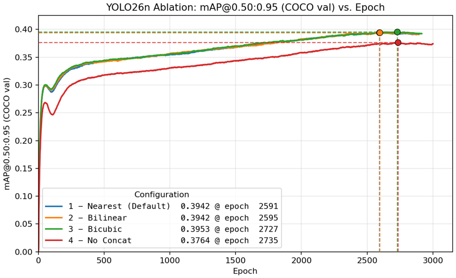
To analyze the effect of the upsampling strategy and concatenation operations, we train four YOLO26n variants from scratch for 3000 epochs on the COCO dataset. Three variants differ only in the interpolation method used for upsampling: (1) nearest neighbor, (2) bilinear, and (3) bicubic. All three achieve similar mAP@0.50:0.95. In the fourth experiment, the concatenation layers are removed and replaced with identity layers to examine the effect of eliminating feature fusion. Figure 20 shows the validation mAP@0.50:0.95 curves over training epochs for the upsampling and feature-fusion ablation variants.

Benchmarking the different interpolation methods on TensorRT 10 (FP16) with an NVIDIA H100 GPU (

Table 5. Upsampling and feature-fusion ablation results for YOLO26n. Bold values indicate the best result in each metric column.

Architecture	Parameters	GFLOPs	mAP@0.50:0.95	Latency (ms)
1—Nearest (Default)	2,572,280	6.1	0.3933 ± 0.00004	0.99 ± 0.04
2—Bilinear	2,572,280	6.1	0.3954 ± 0.00010	0.98 ± 0.01
3—Bicubic	2,572,280	6.1	0.3950 ± 0.00013	1.00 ± 0.02
4—No Concat	2,465,784	5.9	0.3743 ± 0.00009	0.97 ± 0.02

) shows that interpolation choice has a measurable impact on both accuracy and latency. Changing the upsampling mode affects only the interpolation rule, not the learnable structure of the network. For the nearest, bilinear, and bicubic variants, the upsampling layers have zero trainable parameters and preserve the same tensor shapes for a fixed scale factor. Consequently, the surrounding concatenation and convolutional blocks receive tensors with identical dimensions, resulting in identical parameter counts and the same reported convolution-dominated GFLOPs. Any observed latency differences among these upsampling modes should, therefore, be interpreted as backend-specific interpolation effects, such as differences in interpolation kernels, memory-access behavior, scheduling, and hardware utilization, rather than changes in model capacity or convolutional complexity. However, the mAP values can still differ because each interpolation rule resamples feature maps differently before feature fusion, affecting feature alignment and the information passed to subsequent layers.

The default configuration (Model 1, nearest interpolation) achieves 0.3933 mAP@0.50:0.95 with a latency of 0.99 ms, providing solid overall performance. Replacing nearest interpolation with bilinear interpolation (Model 2) yields the best observed result, achieving the highest mAP@0.50:0.95 (0.3954) while also slightly reducing latency to 0.98 ms. Bicubic interpolation (Model 3) also improves accuracy relative to the default configuration, reaching 0.3950 mAP@0.50:0.95, but incurs the highest latency among the interpolation variants at 1.00 ms. Although its accuracy remains close to that of bilinear, it offers no latency advantage, making bilinear the more practical choice of the two. This makes bilinear the most favorable option among the tested interpolation methods in terms of the observed accuracy–latency trade-off.

Finally, removing the concatenation layers (Model 4) slightly reduces latency to 0.97 ms, but causes a substantial drop in accuracy to 0.3743 mAP@0.50:0.95. This indicates that concatenation is important for preserving detection performance, and that eliminating it yields only marginal speed benefits at a significant cost in accuracy. The No Concat variant modifies the feature-fusion structure itself, reducing the input dimensionality of subsequent convolutional blocks; therefore, unlike the interpolation-mode variants, it changes both the parameter count and the reported GFLOPs.

12. Feature Refinement Module (C3k2 with Attention)

12.1. Objective

The C3k2 (attn = True) module is a hybrid feature refinement block in the YOLO26 architecture that combines the efficient partial-channel processing of the C3k2 module with the attention-based contextual modeling of the C2PSA module. Its main purpose is to improve feature quality by jointly capturing:

• Local structural patterns through bottleneck-based convolutional refinement;
• Long-range spatial dependencies through the PSA block;
• Feature preservation through CSP-style split pathways;
• Computational efficiency by applying the most expensive operations to only part of the channels.

Like the standard C3k2 design, the module first divides the feature map into partial paths so that some information is preserved with minimal transformation. However, unlike the C3k2 (False) variant, the transformed branch does not stop at a bottleneck. Instead, it is further refined by a PSA block, allowing the module to combine compact convolutional processing with attention-guided enhancement.

This gives the module several important advantages:

• Partial feature processing: Only a subset of channels is heavily processed, reducing redundancy and improving efficiency.
• Local refinement through the bottleneck: The bottleneck compresses, processes, and restores channels, helping the network emphasize edges, corners, textures, and other localized patterns.
• Global context through attention: The PSA block enriches the refined features with broader spatial relationships, making the representation more aware of distributed object structure.
• Multi-level feature retention: The module preserves an untouched split branch, the pre-attention-processed branch, and the fully refined branch, enabling richer feature fusion.
• Improved optimization: Residual connections in both the bottleneck and the PSA block help maintain information flow and stabilize training.

Overall, the C3k2 (attn = True) module can be viewed as a CSP-style multi-path refinement block that first performs compact local convolutional enhancement and then applies attention-based semantic refinement, producing features that are both efficient and highly expressive.

12.2. Flow

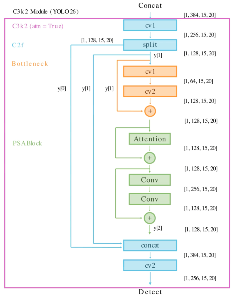
• Initial convolution (cv1): A 1 × 1 convolution is first applied to the input tensor. As seen in Figure 21, the feature map remains at [1, 256, 15, 20], meaning spatial resolution is preserved while the channels are prepared for internal processing.
• Split: The output of the initial convolution is divided along the channel dimension into two equal parts.
• The y[0] branch serves as a preserved shortcut branch that bypasses the heavier transformations and is sent directly toward the final concatenation. The y[1] branch is used as the main refinement path.
• Bottleneck refinement: The y[1] branch first passes through a bottleneck block composed of two convolutions. The first convolution reduces channels from 128 to 64, creating a compressed intermediate representation; the second convolution restores channels from 64 back to 128.
• A residual connection then adds the original y[1] back to the transformed output. This bottleneck stage allows the module to refine local patterns efficiently while preserving the original feature information.
• PSA block refinement: The output of the bottleneck is then passed into a PSA block, which further enhances the features using attention-based processing.
• Inside this PSA block, an attention submodule captures broader spatial dependencies and contextual relationships; its output is added residually to the incoming feature map, and the result then passes through a lightweight two-layer convolutional feed-forward subnetwork. As seen in Figure 21, this subnetwork expands channels from 128 to 256 and then projects them back from 256 to 128; a second residual addition is applied after this feed-forward stage. The PSA block, therefore, refines the bottleneck output by incorporating global context while still preserving the original branch information through internal skip connections.
• Refined output (y[2]): After the bottleneck and PSA block, the final processed branch becomes y[2].
• Concatenation: Three tensors are concatenated along the channel axis: y[0], the preserved shortcut branch; y[1], the original split refinement branch; and y[2], the fully refined branch after bottleneck + PSA processing. This concatenation is important because it preserves raw partial features, intermediate branch features, and deeply refined attention-enhanced features.
• Final convolution (cv2): A final 1 × 1 convolution fuses the concatenated tensor and projects it from 384 channels back to 256 channels, producing the final output of shape [1, 256, 15, 20]. This final step learns inter-channel relationships across all three branches and generates a richer feature representation suitable for the next stage of the network.

To justify the introduction of the new C3k2 configuration in YOLO26, we train three YOLO26n variants from scratch for up to 3000 epochs on the COCO dataset: (1) the original architecture, which employs the new C3k2 configuration with attn = True; (2) a variant with C3k2 set to c3k = False, as examined earlier; and (3) a variant with C3k2 set to c3k = True. Figure 22 shows the validation mAP@0.50:0.95 curves over training epochs for these Stage-22 C3k2 configuration variants.

Benchmarking the final C3k2 module on TensorRT 10 (FP16) with an NVIDIA H100 GPU (

Table 6. Last-stage C3k2 attention ablation results for YOLO26n. Bold values indicate the best result in each metric column.

Architecture	Parameters	GFLOPs	mAP@0.50:0.95	Latency (ms)
1—Last Attn (Default)	2,572,280	6.1	0.3933 ± 0.00004	0.99 ± 0.04
2—Last False	2,454,648	6.0	0.3819 ± 0.00004	0.94 ± 0.02
3—Last True	2,488,056	6.1	0.3921 ± 0.00007	0.97 ± 0.00

) shows a clear accuracy–latency trade-off. The baseline configuration (Model 1, with attn = True) achieves the highest mAP@0.50:0.95 (0.3933) but also has the highest latency (0.99 ms). This indicates that the attention-enabled version provides the best detection performance, although at a modest runtime cost.

Model 2 (attn = False, c3k = False), corresponding to the C3k2 False variant in the final stage, is the fastest configuration at 0.94 ms, but also produces the lowest accuracy (0.3819 mAP@0.50:0.95). Therefore, although this design offers the greatest speed improvement, it does so at a substantial cost in accuracy.

Model 3 (attn = False, c3k = True), which is effectively equivalent to using the C3k2 True variant in the last stage, reduces latency to 0.97 ms while maintaining a relatively high accuracy of 0.3921 mAP@0.50:0.95. This makes it a more balanced alternative than Model 2, since it improves efficiency with only a small reduction in detection performance compared with the baseline.

Overall, the baseline model remains the best accuracy-focused choice, while Model 3 offers the most practical compromise between accuracy and latency. Model 2 is preferable only when minimizing inference time is the primary objective. In this sense, the results support the introduction of the attn flag in YOLO26, as the added bottleneck + PSA structure appears to improve mAP@0.50:0.95 relative to the other C3k2 alternatives.

13. Detection Head

13.1. Objective

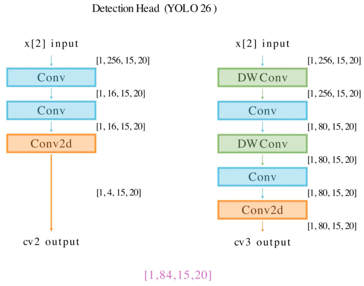
The detection head in YOLO26 is the final stage of the network and is responsible for localizing objects (bounding box regression) and classifying them (category prediction). It receives multi-scale feature maps from the neck (stages 16, 19, and 22 of the feature pyramid network), corresponding to strides of 8, 16, and 32. These inputs allow the head to operate at three different resolutions, ensuring robustness across small, medium, and large objects.

For each feature-map scale, the detection head processes the input feature map through two specialized branches:

• cv2 branch (localization): This branch performs bounding-box regression. Sequential 3 × 3 convolutions refine spatial information, followed by a final 1 × 1 convolution that adjusts the output channels without changing the spatial resolution. The result is a set of four localization values per grid cell, corresponding to the predicted box coordinates.
• cv3 branch (classification): This branch predicts the object category. It uses depthwise separable convolutions, in which spatial filtering is performed independently per channel before pointwise channel mixing. This reduces computation while preserving sensitivity to spatial patterns. For COCO, the branch produces 80 class logits per grid cell, corresponding to the 80 object categories.

After both branches are processed, their outputs are concatenated along the channel dimension. For the COCO setting used in this study, each grid cell, therefore, produces 84 values: 4 for bounding-box regression and 80 for class prediction. This four-value box-regression output follows from the YOLO26n configuration used in this study, where ‘reg_max = 1’. In the Ultralytics Detect module, the DFL module is instantiated only when ‘reg_max > 1’; otherwise, it is replaced by an identity mapping, i.e., ‘self.dfl = DFL(self.reg_max) if self.reg_max > 1 else nn.Identity()’. Therefore, YOLO26n does not use multi-bin Distribution Focal Loss in the detection head.

13.2. Flow

For each input feature map, the detection head applies the localization and classification branches independently. The localization branch produces four box-regression values at each spatial location, while the classification branch produces one logit per class. These branch outputs are then concatenated to form the detection tensor for that feature-map scale.

YOLO26 follows an anchor-free detection formulation. Instead of using predefined anchor boxes, anchor points are generated at the centers of grid cells using an offset of 0.5. The predicted localization values are decoded relative to these anchor points and scaled according to the stride of the corresponding feature map. This converts the grid-level predictions into image-space bounding-box coordinates.

For classification, the raw class logits are mapped to probabilities using a sigmoid function. The decoded bounding boxes and class probabilities together form the candidate detections for each feature-map scale.

For the 480 × 640 network input shown in Figure 6 and used in the detection-head example in Figure 23, the stride-8, stride-16, and stride-32 feature maps contain 60 × 80, 30 × 40, and 15 × 20 grid locations, respectively, resulting in 6300 candidate locations in total. For a 640 × 640 input, the corresponding feature maps contain 80 × 80, 40 × 40, and 20 × 20 grid locations, resulting in 8400 candidate locations. Thus, the number of candidate locations depends on the input resolution and the feature-map strides.

The detection head is retained from the official YOLO26 implementation in this study. Our ablation experiments focus on the architectural components analyzed in the preceding sections rather than on redesigning the detection head itself. Therefore, the Detect module is described here to complete the architectural analysis and clarify the final prediction flow, while the controlled ablations preserve the default YOLO26 detection-head behavior unless otherwise stated.

14. Additional Experimental Analysis

14.1. Best Combined YOLO26n Configuration

To evaluate whether the strongest individual design choices identified in the preceding ablation studies can be combined into a better overall model, we construct and train three candidate YOLO26n combined configurations. These configurations are derived from the most promising variants observed across the SPPF, attention-ratio, and upsampling ablations. The objective of this experiment is to determine whether combining the best-performing components from separate controlled studies yields an improved accuracy–latency trade-off, or whether interactions among the components limit the benefit of combining them.

The three candidate configurations are defined as follows:

YOLO26n Best Config. 1: k = 5, no SPPF shortcut, attention ratio 0.75, and bilinear upsampling.

YOLO26n Best Config. 2: k = 7, with SPPF shortcut, attention ratio 0.75, and bilinear upsampling.

YOLO26n Best Config. 3: k = 7, no SPPF shortcut, attention ratio 0.75, and bilinear upsampling.

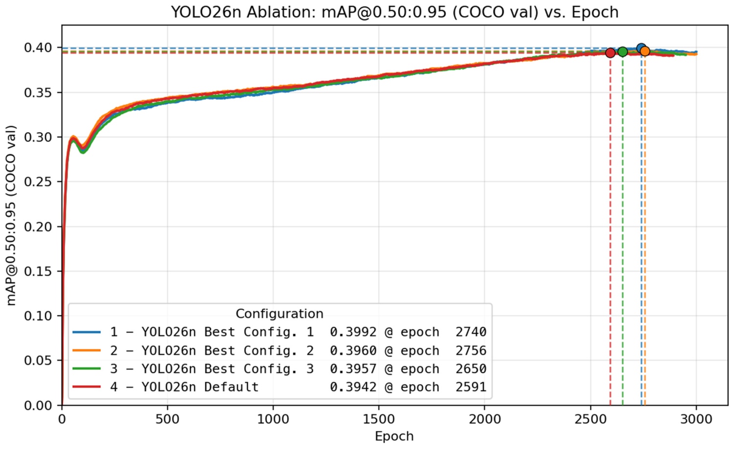
Figure 24 compares the validation mAP@0.50:0.95 curves of the three combined configurations against the default YOLO26n baseline.

As shown in

Table 7. Best combined YOLO26n configuration comparison. Bold values indicate the best result in each metric column.

Architecture	Parameters	GFLOPs	mAP@0.50:0.95	Latency (ms)
1—YOLO26n Best Config. 1	2,580,600	6.2	0.3969 ± 0.00009	1.00 ± 0.05
2—YOLO26n Best Config. 2	2,580,600	6.2	0.3939 ± 0.00008	1.03 ± 0.03
3—YOLO26n Best Config. 3	2,580,600	6.2	0.3958 ± 0.00007	1.00 ± 0.03
4—YOLO26n Default	2,572,280	6.1	0.3933 ± 0.00004	0.99 ± 0.04

, benchmarking the combined configurations with TensorRT 10 FP16 on an H100 GPU shows that YOLO26n Best Config. 1 achieves the highest detection accuracy among the tested models, reaching 0.3969 mAP@0.50:0.95. Compared with the default YOLO26n baseline, this corresponds to an improvement of 0.0036 mAP@0.50:0.95, while increasing latency only marginally from 0.99 ms to 1.00 ms. This indicates that the combination of the default SPPF kernel size, removal of the SPPF shortcut, attention ratio 0.75, and bilinear upsampling provides the most favorable accuracy-oriented improvement with negligible additional inference cost.

YOLO26n Best Config. 3 achieves the second-highest accuracy, with 0.3958 mAP@0.50:0.95 and the same 1.00 ms latency as Best Config. 1. This result suggests that using k = 7 together with no SPPF shortcut, attention ratio 0.75, and bilinear upsampling also improves upon the default baseline, although it does not surpass Best Config. 1. By contrast, YOLO26n Best Config. 2, which retains the SPPF shortcut while using k = 7, attention ratio 0.75, and bilinear upsampling, reaches 0.3939 mAP@0.50:0.95 with a higher latency of 1.03 ms. Although this configuration slightly improves accuracy relative to the default baseline, its increased latency makes it a less favorable trade-off.

The default YOLO26n model remains the fastest configuration, achieving 0.99 ms latency, but it obtains the lowest mAP@0.50:0.95 among the four compared models. Overall, these results show that combining individually favorable architectural choices can improve the final YOLO26n configuration, but the benefit depends on the interaction among components. In particular, Best Config. 1 provides the best overall accuracy–latency trade-off among the evaluated combined configurations.

The best combined configuration improves mAP@0.50:0.95 from 0.3933 to 0.3969, while introducing only a marginal latency increase from 0.99 ms to 1.00 ms under TensorRT FP16 benchmarking. This analysis identifies an improved accuracy–latency trade-off and provides an incremental architectural configuration contribution supported by controlled experiments.

14.2. Model Scaling Analysis

To evaluate whether the improvements identified for YOLO26n generalize beyond the nano-scale model, we extend the best combined configuration to larger YOLO26 variants. Specifically, the same configuration selected in Section 14.1 is applied to YOLO26m and YOLO26l and compared against the corresponding default models under the same controlled training, export, and TensorRT FP16 benchmarking protocol. This experiment addresses whether the observed gains are specific to the lightweight YOLO26n model or remain beneficial across larger model scales.

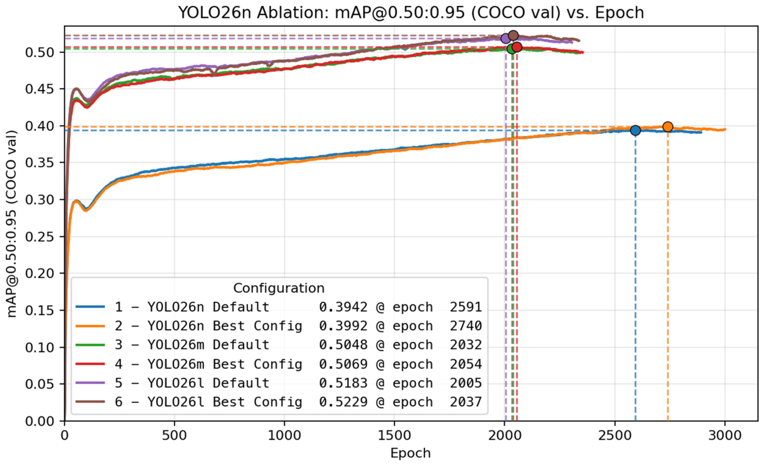
Figure 25 compares the validation mAP@0.50:0.95 curves of the default and best-configuration models across YOLO26n, YOLO26m, and YOLO26l.

Benchmarking the scaled variants with TensorRT 10 FP16 on an H100 GPU shows that the best configuration improves mAP@0.50:0.95 across all three model sizes. For YOLO26n, the best configuration improves mAP@0.50:0.95 from 0.3933 to 0.3969, corresponding to a gain of 0.0036, while latency increases only marginally from 0.99 ms to 1.00 ms. This confirms the result from Section 14.1 that the combined configuration provides a better accuracy-oriented trade-off for the nano model with negligible additional inference cost.

For YOLO26m, the best configuration improves mAP@0.50:0.95 from 0.5033 to 0.5052, corresponding to a gain of 0.0019. Unlike the nano-scale case, this improvement is accompanied by a slight latency reduction from 1.41 ms to 1.39 ms. Thus, for the medium-scale model, the best configuration improves both accuracy and inference speed under the TensorRT FP16 benchmarking setting.

As shown in

Table 8. Cross-scale validation of the best YOLO26 configuration. Bold values indicate the best result in each metric column within each model scale.

Architecture	Parameters	GFLOPs	mAP@0.50:0.95	Latency (ms)
1—YOLO26n Default	2,572,280	6.1	0.3933 ± 0.00004	0.99 ± 0.04
2—YOLO26n Best Config	2,580,600	6.2	0.3969 ± 0.00009	1.00 ± 0.05
3—YOLO26m Default	21,896,248	75.4	0.5033 ± 0.00005	1.41 ± 0.03
4—YOLO26m Best Config	21,929,272	75.5	0.5052 ± 0.00005	1.39 ± 0.01
5—YOLO26l Default	26,299,704	93.8	0.5155 ± 0.00004	1.84 ± 0.04
6—YOLO26l Best Config	26,365,752	93.9	0.5200 ± 0.00005	1.85 ± 0.04

, for YOLO26l, the best configuration improves mAP@0.50:0.95 from 0.5155 to 0.5200, corresponding to a gain of 0.0045. The latency increases only marginally, from 1.84 ms to 1.85 ms. This result indicates that the selected configuration also benefits the large-scale model, although the improvement should be interpreted as an incremental refinement rather than a major architectural change.

Overall, these results show that the best combined configuration is not limited to YOLO26n. Although the magnitude of the improvement varies across scales, the best configuration consistently improves mAP@0.50:0.95 for YOLO26n, YOLO26m, and YOLO26l. The latency impact is also small across all three variants, with either negligible increases or a slight reduction in the case of YOLO26m. This cross-scale validation supports the conclusion that the identified configuration changes generalize beyond the nano model while preserving the deployment-oriented efficiency of the YOLO26 family.

The cross-scale comparison confirms that the best combined configuration improves detection accuracy across YOLO26n, YOLO26m, and YOLO26l. The gains are modest but consistent, increasing mAP@0.50:0.95 by 0.0036, 0.0019, and 0.0045 for YOLO26n, YOLO26m, and YOLO26l, respectively. Because the associated latency changes are negligible, these results provide additional evidence that the selected configuration offers a favorable accuracy–latency trade-off across multiple YOLO26 model scales.

14.3. Comparison with YOLO11n

To provide external context beyond the internal YOLO26n ablation studies, we compare the default and best-configuration YOLO26n models against corresponding YOLO11n variants. This comparison addresses whether the final YOLO26n configuration is competitive with another widely used nano-scale YOLO-family detector under the same controlled training, export, and deployment-backend evaluation protocol. All models are trained from scratch on COCO using the same training configuration, including MuSGD, and are evaluated after TensorRT FP16 export on the same NVIDIA H100 GPU. Therefore, the YOLO11n results in this comparison should be interpreted as results for the YOLO11n architectural configurations trained under our controlled recipe, rather than as off-the-shelf Ultralytics checkpoints or reproductions of the original Ultralytics headline benchmarks.

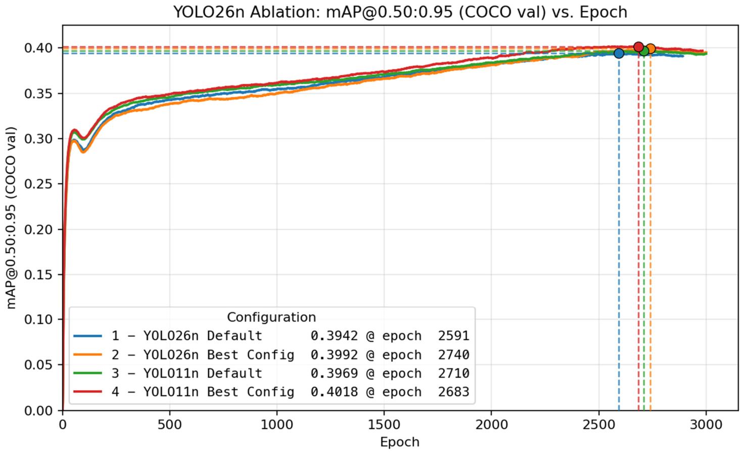
The purpose of this comparison is not to claim universal state-of-the-art superiority, because reported performance rankings can depend strongly on training recipes, pretraining assumptions, export settings, inference backend, and hardware. Instead, the comparison provides a controlled horizontal reference under the fixed experimental protocol used throughout this work, with the goal of assessing architecture/configuration behavior under a matched MuSGD-based training and TensorRT FP16 deployment protocol.

Figure 26 compares the validation mAP@0.50:0.95 curves of the default and best-configuration variants of YOLO26n and YOLO11n.

As shown in

Table 9. Horizontal comparison between YOLO26n and YOLO11n under the controlled COCO-only TensorRT FP16 evaluation protocol on an NVIDIA H100 GPU. ‘Default’ denotes the default architecture for each model family trained from scratch under the same controlled recipe, including MuSGD, rather than an off-the-shelf pretrained Ultralytics checkpoint. ‘YOLO11n Best Config’ uses the transferred configuration settings documented in Appendix A. Bold values indicate the best result in each metric column.

Architecture	Parameters	GFLOPs	mAP@0.50:0.95	Latency (ms)
1—YOLO26n Default	2,572,280	6.1	0.3933 ± 0.00004	0.99 ± 0.04
2—YOLO26n Best Config	2,580,600	6.2	0.3969 ± 0.00009	1.00 ± 0.05
3—YOLO11n Default	2,624,080	6.6	0.3965 ± 0.00005	0.89 ± 0.03
4—YOLO11n Best Config	2,632,400	6.6	0.4019 ± 0.00004	0.86 ± 0.02

, the best YOLO26n configuration improves mAP@0.50:0.95 from 0.3933 to 0.3969, corresponding to a gain of 0.0036, with only a marginal increase in latency from 0.99 ms to 1.00 ms. This confirms the internal ablation result that the selected configuration improves the YOLO26n baseline with negligible additional inference cost.

For reproducibility, YOLO11n Best Config is defined relative to the YOLO11n Default baseline instantiated in the same Ultralytics 8.4.6 codebase and trained under the same controlled protocol used for YOLO26n, rather than relative to an external off-the-shelf YOLO11n checkpoint or a different Ultralytics release. The YOLO11n Best Config was constructed by replacing the YOLO11n Default YAML reference with the corresponding best-configuration YAML while keeping the same training invocation, dataset, seed, epoch budget, early-stopping rule, optimizer selection, export procedure, and TensorRT FP16 benchmarking protocol. Under ‘optimizer = auto’, both the YOLO26n Best Config and YOLO11n Best Config runs resolved to MuSGD with learning rate 0.01 and momentum 0.9. The transferred architectural settings were SPPF without shortcut, attention ratio 0.75, and bilinear upsampling with ‘align_corners = False’. In the YOLO11n YAML, bilinear upsampling is explicit in the two neck upsampling layers. The SPPF no-shortcut setting follows from the SPPF constructor default ‘shortcut = False’ when the layer is specified as ‘SPPF, [1024, 5]’, which is equivalent in this implementation to ‘SPPF, [1024, 5, 3, False]’. The attention-ratio setting is not exposed as a YAML argument in this implementation and is, therefore, documented in Appendix A as an implementation-level setting. The YOLO11n Best Config YAML, parsed model summary, and implementation notes are provided in Appendix A.

For YOLO11n, applying the transferred best-configuration settings also improves performance, increasing mAP@0.50:0.95 from 0.3965 to 0.4019. This corresponds to a gain of 0.0054. In addition, latency decreases from 0.89 ms to 0.86 ms under the TensorRT FP16 H100 benchmarking setting. This result shows that, under the controlled MuSGD-based training and TensorRT FP16 deployment protocol used here, the same documented configuration changes improve both the YOLO26n baseline and the corresponding YOLO11n baseline.

The horizontal comparison also shows that YOLO11n achieves stronger overall results than YOLO26n in this specific deployment setting. In Table 9, ‘YOLO11n Default’ denotes the default YOLO11n architecture trained from scratch under the same controlled COCO-only recipe used for the YOLO26n experiments, including MuSGD, rather than an off-the-shelf pretrained Ultralytics YOLO11n checkpoint or a reproduction of the original Ultralytics headline benchmark. The two model families use the same dataset, image size, batch size, epoch budget, early-stopping rule, augmentation settings, seed, hardware configuration, and optimizer selection; in both cases, optimizer = auto resolves to MuSGD (lr = 0.01, momentum = 0.9). The remaining differences, therefore, arise from the respective YOLO11n and YOLO26n YAML architecture definitions, including differences in layer count, detection-head structure, parameter count, and GFLOPs. Under this protocol, YOLO11n Default achieves slightly higher mAP@0.50:0.95 than YOLO26n Default while also running faster, and YOLO11n Best Config achieves the highest mAP@0.50:0.95 and the lowest latency among the four evaluated models. Therefore, these results should not be interpreted as showing that YOLO26n is universally superior to other nano-scale detectors. Rather, they show that the proposed configuration analysis improves YOLO26n relative to its own default baseline and that the transferred configuration is also beneficial for the corresponding YOLO11n baseline under the controlled MuSGD-based training and TensorRT FP16 deployment protocol used here. This supports the value of the proposed analysis as a deployment-oriented architectural attribution method rather than as a SOTA claim.

The lower YOLO11n latency, despite its slightly higher nominal GFLOP count, suggests that FLOPs alone do not explain the observed deployment behavior. Although YOLO11n and YOLO26n share a similar high-level P3/P4/P5 detection topology, their YAML definitions differ in deployment-relevant details, including the YOLO26n end-to-end setting, the reg_max = 1 detection-head configuration, and different C3k2 settings in the head. These differences may affect the exported TensorRT graph, operator mix, memory-access behavior, fusion opportunities, or tactic selection, which could contribute to the observed latency difference. This interpretation is mainly relevant to latency; the mAP difference may instead reflect architectural and optimization factors. Because this work does not include dedicated TensorRT layer-timing, kernel-fusion analysis, or hardware-counter profiling, we treat this explanation as a plausible deployment-backend hypothesis rather than as a definitive causal conclusion.

The comparison provides two important observations. First, the best-configuration changes improve both YOLO26n and YOLO11n under the same MuSGD-based training and TensorRT FP16 benchmarking protocol, increasing the mean mAP@0.50:0.95 by 0.0036 and 0.0054, respectively. Second, YOLO11n remains the stronger nano-scale model in this particular TensorRT FP16 H100 evaluation, achieving both higher accuracy and lower latency. These findings clarify the scope of the contribution: the proposed study does not claim overall state-of-the-art superiority or Pareto-frontier dominance for YOLO26n but instead provides a controlled architectural analysis showing how YOLO26n can be improved relative to its own baseline and how the same documented configuration changes perform when applied to a corresponding YOLO11n baseline under the tested protocol.

15. Conclusions

This paper presented a block-level, modular analysis of YOLO26n, clarifying the objective, internal flow, and representational transformations of its primary components, from convolutional stems and bottleneck-style refinement blocks to multi-scale aggregation and attention mechanisms. By decomposing the network into interpretable building blocks and explicitly tracking tensor shape evolution, we provide a practical technical reference that connects architectural design intent to observable feature transformations.

In addition to architectural interpretation, we introduced a controlled ablation suite designed to quantify the marginal contribution of key design choices under a fixed, fully specified training and benchmarking protocol. Across ablations spanning activation functions, C3k2 variants, SPPF settings, attention configurations, and related implementation choices, we measured the impact of each change on COCO mAP@0.50:0.95 and TensorRT FP16 inference latency. By changing one factor at a time while holding the dataset, training schedule, export procedure, and benchmarking configuration fixed, this study isolates which modules provide meaningful accuracy–efficiency gains and which offer limited return under the tested constraints.

Beyond isolated ablations, we evaluated combined YOLO26n configurations derived from the strongest individual findings. This step is important because module-level improvements are not necessarily additive when applied together. Under the fixed seed-0, COCO-only training-from-scratch and TensorRT FP16 H100 benchmarking protocol used in this work, the best combined YOLO26n configuration improves mAP@0.50:0.95 from 0.3933 to 0.3969, while increasing latency only marginally from 0.99 ms to 1.00 ms. This result shows that the ablation findings can be translated into an incremental architectural refinement, rather than serving only as diagnostic observations.

To evaluate whether this refinement is limited to the nano-scale model, we further applied the best combined configuration to larger YOLO26 variants. The cross-scale validation shows consistent accuracy improvements across YOLO26n, YOLO26m, and YOLO26l. Specifically, mAP@0.50:0.95 increases by 0.0036 for YOLO26n, 0.0019 for YOLO26m, and 0.0045 for YOLO26l, with negligible latency changes under the same TensorRT FP16 H100 evaluation protocol. These results provide limited cross-scale evidence within the YOLO26 family, indicating that the selected configuration changes are not restricted to the nano-scale model under the tested COCO-based training and evaluation setting.

A horizontal comparison with YOLO11n provides external context beyond internal YOLO26-family comparisons. Under the controlled COCO-only, MuSGD-based training and TensorRT FP16 H100 evaluation protocol used in this work, YOLO11n achieves stronger overall results than YOLO26n, with YOLO11n Best Config reaching 0.4019 mAP@0.50:0.95 and 0.86 ms latency. We emphasize that the YOLO11n results correspond to YOLO11n architectural configurations trained from scratch under the same controlled recipe as the YOLO26n experiments, including MuSGD, rather than off-the-shelf Ultralytics checkpoints or reproductions of the original Ultralytics headline benchmarks. This finding is important because it clarifies the scope of the contribution: the goal of this work is not to claim that YOLO26n is universally superior to other nano-scale detectors, Pareto-dominant over YOLO11n, or a new state-of-the-art result. The observed YOLO11n latency advantage may partly reflect TensorRT FP16 backend interactions with the YAML-defined detection/head structure, although this work does not perform kernel-level profiling and, therefore, does not claim a definitive low-level runtime cause. Rather, the contribution is a controlled architectural attribution and configuration-refinement study showing how YOLO26n can be improved relative to its own default baseline. Thus, the paper contributes a controlled block-level architectural attribution study of YOLO26, including one-factor-at-a-time ablations, combined-configuration refinement, cross-scale validation, and horizontal comparison under a fixed COCO-only training and TensorRT FP16 benchmarking protocol, rather than proposing a new detector family, a new detector architecture, or a license-free alternative implementation. The YOLO11n comparison further shows that similar configuration changes can improve another nano-scale YOLO-family model, increasing mAP@0.50:0.95 from 0.3965 to 0.4019 while reducing latency from 0.89 ms to 0.86 ms under the same MuSGD-based training and TensorRT FP16 deployment setting.

To avoid conflating architectural effects with recipe and data effects, all experiments are trained from scratch using seed 0 on MS COCO train2017 and evaluated on val2017 under the same controlled MuSGD-based recipe. We explicitly distinguish this COCO-only setting from headline benchmarks that may rely on external-data pretraining, off-the-shelf pretrained checkpoints, larger training recipes, different datasets, or different deployment hardware. Consequently, the results should be interpreted as controlled single-seed comparisons under a fixed experimental protocol rather than as statistically validated multi-seed estimates, reproductions of official Ultralytics headline benchmarks, or universal rankings across all YOLO-family detectors. In addition, the fixed recipe was not individually optimized for each ablation variant. Thus, conclusions such as one activation function or module configuration outperforming another should be understood within the shared training protocol used here, not as claims about the maximum achievable performance of each variant under separately tuned hyperparameters. Dataset-level external validity is not established in this work, since the experiments remain COCO-based. Evaluation on additional datasets, downstream domains, deployment platforms, targeted per-variant hyperparameter tuning, and full multi-seed validation is, therefore, an important direction for future work.

The practical use of the analyzed implementation is also subject to licensing constraints. Because the experiments rely on the official Ultralytics YOLO26 implementation, use, reproduction, modification, redistribution, or deployment of YOLO26-based models remains subject to the applicable Ultralytics licensing terms. In particular, Ultralytics YOLO code and trained models are distributed under AGPL-3.0 by default, while certain proprietary commercial uses may require an appropriate Ultralytics Enterprise License.

The analysis workflow used here, combining Objective → Flow interpretation, tensor tracking, standardized ablations, combined-configuration evaluation, cross-scale validation, and horizontal model comparison, may be applied beyond YOLO26n. However, the specific numerical findings reported in this study should be interpreted within the tested scope: YOLO26-family models and YOLO11n, trained from scratch using seed 0 on MS COCO under the controlled MuSGD-based recipe and evaluated using the specified TensorRT FP16 H100 protocol. As real-time detection architectures continue to evolve rapidly, such structured attribution studies can help researchers and practitioners evaluate which architectural changes drive improvements under controlled conditions and whether those changes transfer across model scales, related architectures, datasets, and deployment environments.