Data-Driven Analysis of the Effect of Agrivoltaics Systems on Soil and Air Conditions—A Case Study in Kressbronn, Germany

Abstract

Agrivoltaics (AV), the dual use of land for solar power generation and agricultural production, offers a sustainable strategy for optimising land resources. Overhead photovoltaic (PV) modules can change microclimatic conditions, thereby influencing soil moisture, soil temperature, and air temperature and humidity. This study assessed the impact of AV systems on air and soil conditions in a pilot apple orchard in Kressbronn im Bodensee (Bodenseekreis district, Baden-Württemberg, Germany). A semi-transparent PV system (40% transparency) was installed, and soil and air parameters were continuously monitored between August 2024 and August 2025. The results show that AV increased average soil moisture by 11.8% and decreased average soil temperature by 0.8 °C compared to the reference area from a one-year period (August 2024 up to August 2025). Air temperatures beneath the modules were +0.2 °C higher in the early morning but lower (−0.5 °C) at midday during the warmer season. Relative humidity beneath the PV modules showed a diurnal pattern, with higher values than the open reference during nighttime and early morning hours, and lower values during certain daytime windows, resulting in an overall mean difference of −2.2%. These findings confirm that AV installations substantially alter microclimatic conditions, with potential implications for orchard management and crop productivity.

1. Introduction

Significant progress in solar PV technology has made it possible to use this vast, clean energy source. The International Energy Agency (IEA) predicts that by 2050, solar PV will generate 6000 TWh, supplying 16% of the world’s total electricity [1]. To achieve this, we need to cover extensive areas with solar panels. While building-integrated PV and rooftop systems can meet much of the demand, land-based solar farms [2] are necessary. However, this creates a conflict: both food and electricity generation by PV need land, and this competition is especially fierce in densely populated or geographically limited regions.

AV is an innovative land-use strategy that merges PV energy systems with active agriculture on the same land [3]. This approach addresses the growing competition for land between food production and renewable energy infrastructure by allowing both to coexist and run simultaneously [4]. The strategic placement of elevated and semi-transparent PV panels over crops facilitates continued plant growth while generating electricity. Researchers have shown that this integration increases the economic value of farms by over 30% compared to traditional agriculture [5] and has produced a Land Equivalent Ratio (LER) above 1.2 [6]. A LER greater than 1.0 shows that the combined system is more efficient than growing crops and generating solar power on separate land areas. AV systems’ success in improving agricultural productivity is tied to their design, and designers must tailor the design to specific climate conditions and crop light requirements. In 2021, people estimated the global AV sector’s value at USD 3.6 billion, and they project it will reach USD 9.3 billion by 2031 [7], highlighting its growing importance in achieving national sustainability goals.

Overhead AV refers to a specific AV system in which someone installs solar panels on elevated structures above the ground, allowing agricultural activities to occur underneath. From the perspective of photosynthetically active radiation (PAR) distribution, the interspace agrivoltaic (AV) configuration was preferred over the overhead system, as it provides a more uniform and balanced spatial allocation of light within the crop canopy, reducing excessive shading directly above the plants and improving overall light availability for photosynthesis [8]. Other works focused on improving any other parameters, such as installing free-swinging PV (generating 12% more energy than vertical or fixed-tilt PV systems) [9] or proposing a height of 2.5 m as the most optimal for planting figs and similar fruit trees in AV systems [10].

In addition to co-locating food and energy production, AV systems induce measurable modifications to the microclimatic environment beneath the PV arrays. By altering incident solar radiation, wind speed, air temperature, and relative humidity, these systems influence both the abiotic and biotic conditions experienced by crops. Shading from PV modules can mitigate thermal and radiative stress, reduce evapotranspiration rates, and enhance soil moisture retention, potentially improving plant water-use efficiency under water-limited conditions [11].

On the other hand, the disadvantages are the impacts of shading on crop growth [12] and microclimatic conditions under the array. Even moderate shading might lead to severe loss in harvest and quality. This reduction in solar radiation was quantified as over 40% [13], although they also showed that AV with a cover ratio equal to or lower than 25% did not show significant effects on plant growth and quality. The response of crops to the shading from AV systems varies significantly. While most crops can tolerate up to a 15% reduction in solar radiation [14] with a minimal impact on yield, optimal shade levels are highly crop-specific. Also, in apple trees [15], the effect of shading was identified, which reduced the fruit weight by 16%, as was the influence of AV installations in maturation patterns of the crops. For instance, fruits, berries and fruity vegetables often benefit from a solar radiation reduction of up to 30% [14]. Other crops, leafy vegetables, forages, root crops, and C3 cereals show only minor yield losses. However, certain crops like maize and grain legumes are particularly sensitive to shading and can suffer significant yield losses even at low shade levels.

Research on the hydrological effects of solar farms is still developing, but some studies [16] indicate that the shading from solar panels can lead to lower average soil and air temperatures compared to full-sun areas. In Mediterranean regions, AV systems have been shown to reduce water loss from evaporation [17] and help mitigate crop stress. Low soil moisture is a significant problem for plant growth, as it causes drought stress that impairs a plant’s ability to photosynthesise and absorb nutrients, ultimately stunting growth and reducing crop yield. Dry soil is also more prone to erosion. While some studies suggest that soil moisture might be higher under solar panels [18], other factors, such as altered wind speed, direction, and relative humidity—expected to increase [19]—around the panels can also influence the microclimate [20]. Overall, a comprehensive understanding of the impact of AV on hydrology, including runoff and erosion, is still emerging.

Modern sensors now collect real-time data on key environmental factors such as temperature, humidity, soil moisture, and light intensity, enabling informed decision-making in crop management [21]. These IoT-based systems transmit field data to cloud platforms, where they can be analysed [22]. Research shows that such systems improve agricultural productivity and resource efficiency [23]. By enabling real-time monitoring of vital conditions, they allow farmers to track field status remotely, receive timely alerts about critical issues, and optimise their farming practices.

This manuscript investigates how overhead AV systems influence the microclimate. The study aims to answer the following questions:

• Soil moisture: How does coverage by PV modules alter soil moisture, and are there detectable edge effects at module boundaries?
• Soil temperature: How do PV modules change soil temperature at the surface and within the upper soil profile?
• Air temperature and humidity: What effect do PV modules have on near-surface air temperature and relative humidity within the AV installation?
• Drip edge effects: Do soil moisture and soil temperature at the PV drip edge differ from those under the panel interior and in fully exposed areas?

To answer these questions, research was performed in 2024–2025 at a pioneering AV installation near Lake Constance in southwestern Germany. In the town of Kressbronn am Bodensee, the 0.4-hectare site is part of a broader agricultural region known for its apple production, benefiting from a temperate climate shaped by both alpine geography and the microclimatic influence of the lake. This dual-use site is a key component of the Modellregion Agri-PV BaWü (Grant Agreement No. L75 22114) and its subproject StaMoMo (Standard Monitoring of Modellregion Agri-PV BaWü). It features semi-transparent glass–glass modules (260 W), which allow 40% light transparency to reach the apple trees below.

This research provides valuable insights for a broad audience, including researchers, industry practitioners, and policymakers. The findings directly apply to any AV installation in similar climate conditions. Because of the flexibility of the method, it has potential for wider application in regions with varying water demands and solar radiation levels, where outcomes may differ. Several limitations should be considered. First, the study lacks true experimental replication, relying on a single comparison between one under-panel zone and one open-field reference, with no pre-installation baseline to confirm their initial equivalence; thus, results indicate associations rather than proven causality. Accordingly, the findings presented here should be interpreted as spatial associations rather than evidence of causal mechanisms, consistent with the objectives stated in our study. We recognise that establishing causality would require more robust experimental frameworks, such as randomised block designs or long-term before–after control–impact (BACI) designs incorporating baseline data and multiple reference sites. Second, the dataset covers only one year (August 2024–August 2025), limiting assessment of interannual variability. Third, no measurements of PAR or solar irradiance were taken, so links between microclimate changes and radiative forcing remain indirect, and the 40% transmittance is based on manufacturer data. Fourth, energy production was not measured, preventing evaluation of the energy–microclimate trade-off. Fifth, the spatial resolution of soil sensors (10 cm) may miss sharp gradients near the panel edge. Finally, results are specific to this system and climate and should not be generalised without further validation.

2. Materials and Methods

2.1. Study Area

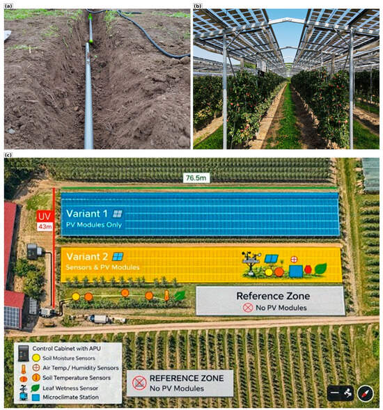
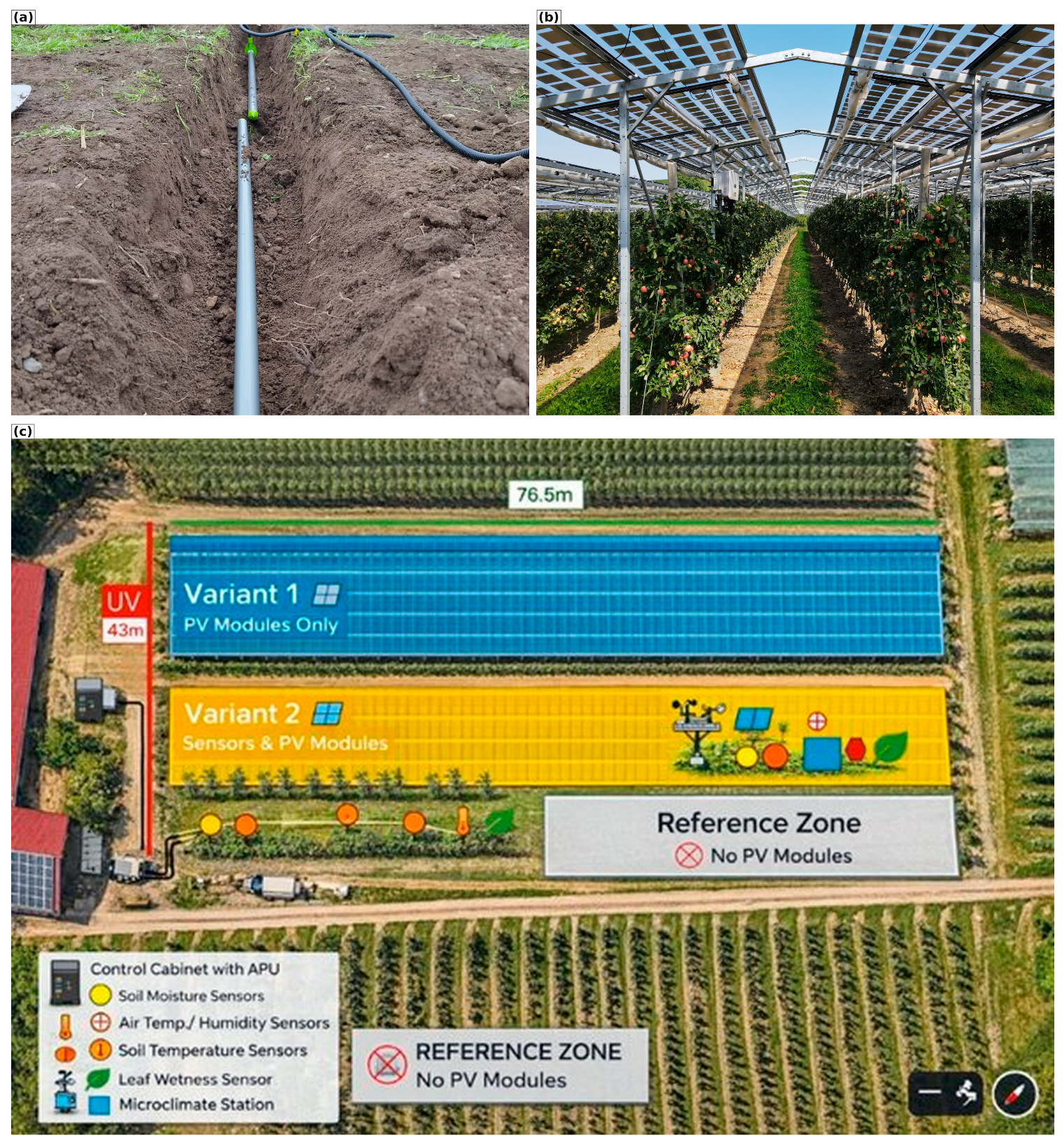
The study was conducted in an apple orchard in Kressbronn am Bodensee (9.60425° E, 47.6017° N, WGS 84), a town in southwestern Germany. Located near the shores of Lake Constance, the region’s temperate climate, influenced by both alpine geography and the lake’s microclimate, makes it a prime area for apple production. This favourable setting, combined with a long-standing agricultural tradition, makes the site an ideal location for evaluating the performance of AV systems under dynamic environmental conditions. This dual-use site underwent continuous monitoring to assess both solar energy production and agricultural performance (Figure 1).

2.2. Data Collection

The bottom of Figure 1 illustrates the area where the sensors are installed. In the zone designated as Variant 2, the sensors are located beneath the PV modules. The agrivoltaic installation at Kressbronn uses semi-transparent glass–glass photovoltaic modules (260 W peak power) based on crystalline silicon (c-Si) cell technology. The semi-transparency arises from the defined inter-cell spacing within the dual-glass laminate: the c-Si cell areas are fully opaque, absorbing strongly across the PAR (400–700 nm) and NIR (700–1100 nm) wavebands, while the inter-cell gaps transmit solar radiation with minimal spectral modification. The resulting module-level transmittance of approximately 40% represents the area-weighted average of these opaque and transparent regions. Importantly, this figure describes broadband attenuation rather than spectrally selective filtering, meaning the radiation transmitted to the surface beneath retains a spectral composition broadly similar to ambient sunlight. This distinguishes the c-Si glass–glass modules from thin-film or organic semi-transparent PV technologies, which can alter the red-to-far-red ratio in agronomically significant ways. The primary optical effect on the under-panel microclimate is therefore a uniform ~60% reduction in total irradiance, with proportional consequences for net radiation, soil heating, and evapotranspiration demand. In contrast, in the reference or control area (REF, shown in grey, Figure 1), the sensors are not influenced by the AV installation.

2.2.1. Sensors for Soil Moisture and Soil Temperature

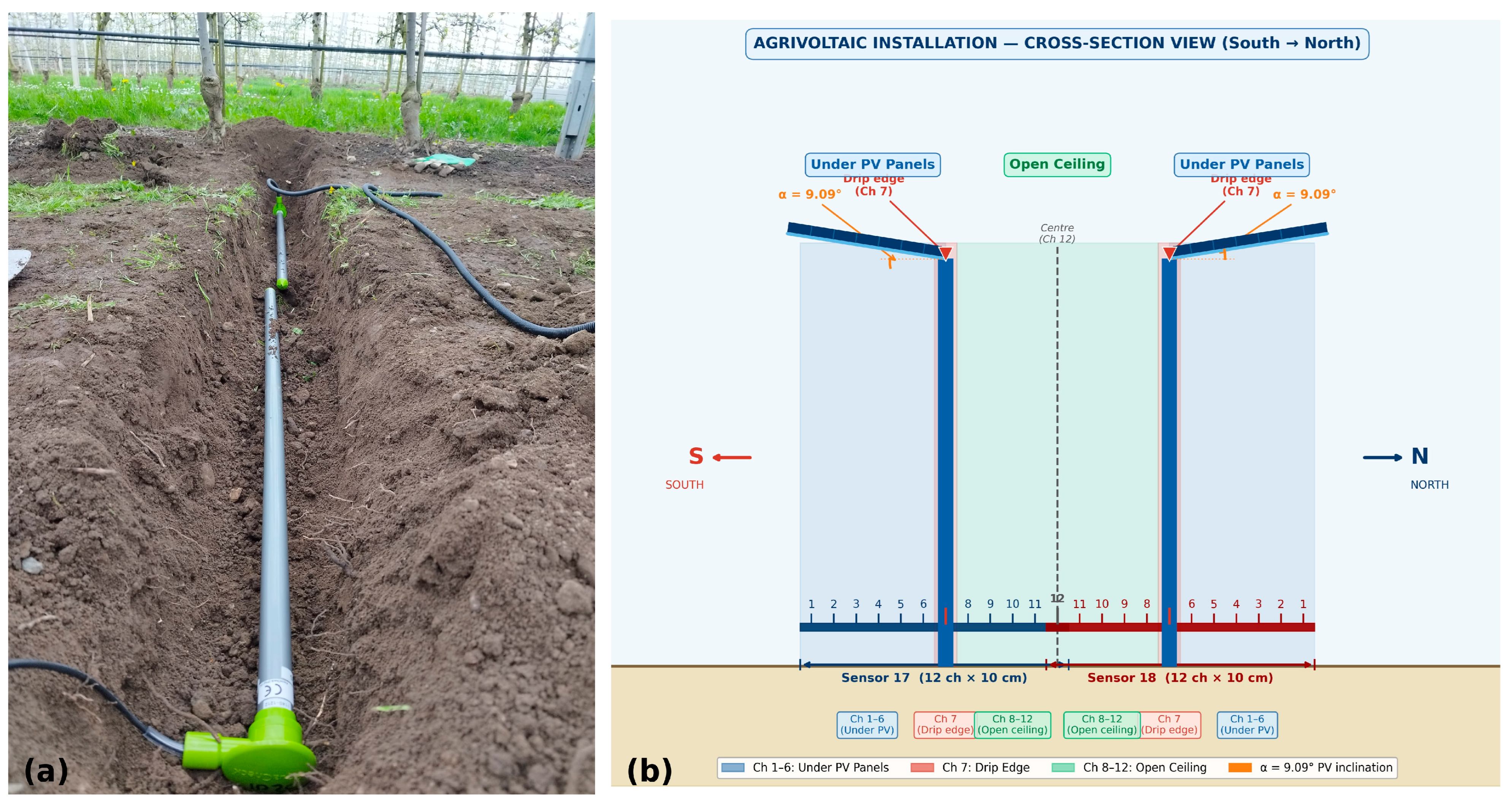
Six horizontal soil sensors (Aquacheck Soilprobe 120 cm, Soil Moisture Management AquaCheck (Pty) Ltd., Brackenfell, South Africa), which gather data every 2 min, were installed one against the other as shown in Figure 2a. The data selected for this analysis were from 28 March 2024 up to 08 August 2025 (204,610 values for the horizontal sensors). The sensors numbered 17 and 18 (buried to a depth of 20 cm) are depicted in Figure 2. It is important to note that sensors 21 and 22 are within the control area highlighted in Figure 1c, where there are no PV modules affecting these sensors. Figure 2 illustrates the specific measurements for the AV installation, where the spacing between rows of apple trees is 3 m. Each sensor is installed horizontally and oriented perpendicular to the PV module rows. Each sensor comprises 12 individual measurement points (hereafter referred to as channels), spaced 10 cm apart, thereby providing 12 discrete readings along the sensor. The total sensor length (Figure 2) is 1200 mm. Field measurements indicate that the tilt angle of the PV modules is α = 9.09°. Considering this tilt and the PV module length of 2006 mm, channels 1–6 are beneath the PV modules, channel 7 coincides with the drip edge, and channels 8–12 are positioned in the open-ceiling area. Additionally, rainwater falling on the PV modules may be conveyed toward the exposed section of the horizontally installed sensors.

2.2.2. Climatic Stations for Relative Humidity and Air Temperature

Four sensors were installed at the Kressbronn pilot plant.

Table 1. Location of the microclimatic stations.

Height (m)	Under PV Modules	Open Ceiling
2	Sensor 1	Sensor 3
5		Sensor 2
20 cm under the PV modules	Sensor 4

displays the locations of the sensors, differentiating between the installation height and whether the sensor is positioned below PV modules or under an open ceiling.

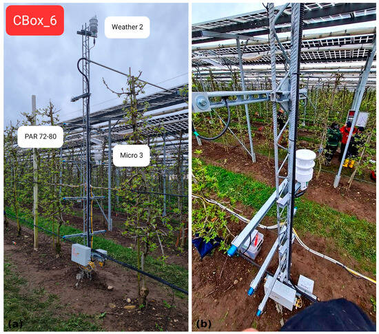
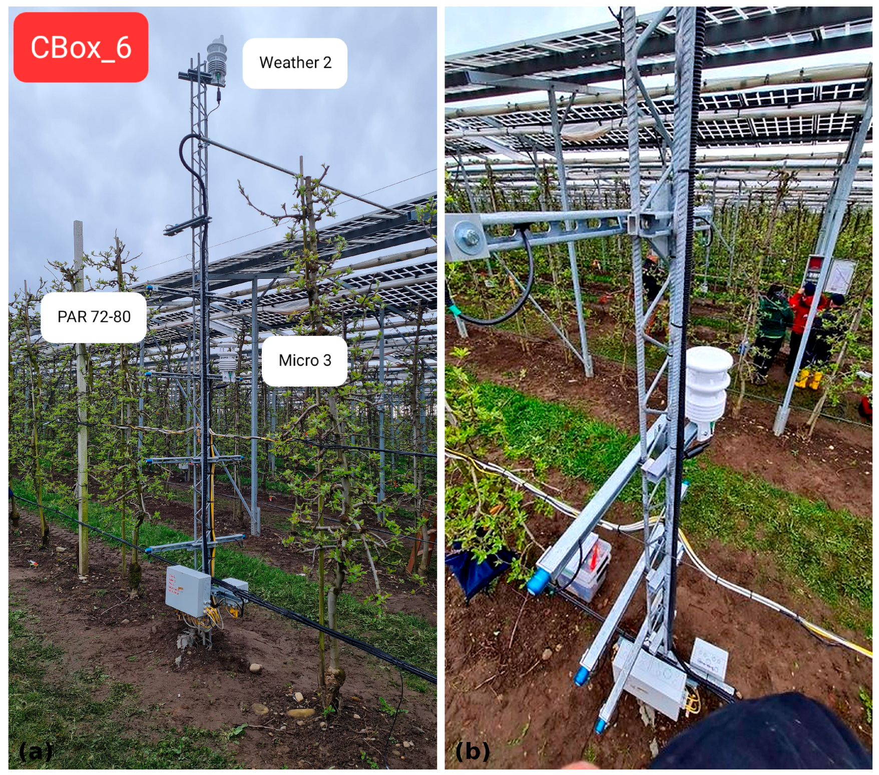
The microclimate station WS500-UMB sensors from Lufft were installed at the points Micro 1, 2, and 3 (Figure 3b), while the weather station WS700-UMB sensor from Lufft was installed at Weather 2 (Figure 3a). Both models measure temperature within a range of −50 °C to +60 °C, with an accuracy of ±0.2 °C (−20 °C to +50 °C), and relative humidity from 0% to 100%, with an accuracy of ±2%. At sensor 4 (Table 1), a reference cell from IMT was installed. The specific model, Si-RS485TC-2T-MB, features an external ambient temperature sensor with a measurement range of −25 °C to +75 °C and an accuracy of ±5%. It also incorporates temperature compensation to enhance measurement accuracy.

2.3. Data Processing

2.3.1. Removing Outliers and Filtering

The initial phase of data processing involves a systematic approach to identify and eliminate outliers within the dataset. Outliers can significantly skew analytical results and lead to misleading conclusions, making their removal crucial for maintaining data integrity.

2.3.2. Air and Soil Temperature Data

Outliers in the database were removed by retaining only temperature values within the range of −20 °C to 50 °C. This threshold was established based on domain knowledge and previous studies, which indicate that such extremes are improbable under normal environmental conditions. Subsequently, a statistical cleaning step was applied based on a maximum allowable temperature change of 1 °C per minute. For this purpose, we used the Hampel filter [24], a statistical method for detecting and replacing outliers in time-series data. This filter identifies values that deviate significantly from a moving median, using a defined window size and threshold. Specifically, for each data point, the median and the median absolute deviation (MAD) are calculated within the selected window, and any values deviating from the median by more than the threshold are replaced.

2.3.3. Relative Humidity and Soil Moisture Data

Outliers in the database were removed by retaining only humidity (or soil moisture) values within the range of 0% to 100%. This is a standard range for relative humidity and volumetric water content, where values beyond this range are considered unrealistic and indicative of sensor errors or data entry mistakes. Similarly to temperature data, a statistical cleaning step was applied based on a maximum allowable humidity (or soil moisture) change of 1% per minute, using the Hampel filter.

2.3.4. Fourier Transform

Spectral analysis via Fourier transform was selected to characterise the periodic structure of the four microclimate variables—soil temperature, soil moisture, air temperature, and air humidity—measured beneath and outside the PV modules. This choice was motivated by the physical nature of AV systems: PV panels impose a structured, quasi-periodic modulation on incoming solar radiation. This structured forcing means that the microclimate signals beneath the modules are expected to carry multiple superimposed periodicities simultaneously, including a dominant diurnal cycle (~24 h), potential sub-diurnal harmonics arising from the morning-to-afternoon evolution of panel shading geometry, and lower-frequency seasonal trends. While time-series plots can reveal the overall temporal behaviour of these variables, visual inspection alone cannot reliably decompose overlapping cycles of different frequencies and amplitudes, nor can it quantify whether the presence of the PV installation systematically alters the energy distribution across these frequency components.

Fourier transform addresses this limitation by converting the time-domain signal into the frequency domain, allowing the spectral power at each frequency to be quantified and directly compared between under-panel and open-field positions. The frequencies of primary interest are the diurnal harmonic (f = 1 day⁻¹) and its higher-order harmonics, since these capture the daily thermal and moisture cycles that are most directly modulated by panel shading. By comparing power spectra between positions, this analysis reveals whether the PV modules dampen the amplitude of the diurnal peak in soil temperature—consistent with a thermal buffering effect—or redistribute spectral power toward sub-daily frequencies in humidity, as might arise from condensation and evaporation dynamics beneath the panels. These are mechanistic insights into AV microclimate modification that time-series visualisation alone cannot provide.

2.4. Statistical Analysis

Data were processed using custom scripts in Python 3.12 with the following libraries: pandas, numpy, seaborn, datetime, scipy, and matplotlib. The panda library was used for data manipulation and cleaning, including reading Excel files. Statistical analyses and summaries were performed using functions from scipy, and visualisations were created with matplotlib. These packages are all available from the Python Package Index (PyPI) at https://pypi.org.

This statistical analysis focused on horizontal soil sensors, comparing those installed beneath the photovoltaic (PV) modules (sensors 17–20; variant 2 in Figure 1) with sensors located in the reference area (sensors 21–22; Figure 1), which is unaffected by the modules. Measurements from these two locations constitute independent samples grouped by position. Air humidity and air temperature data were obtained directly from microclimate station 3, as a single measuring device served both variables (Figure 3).

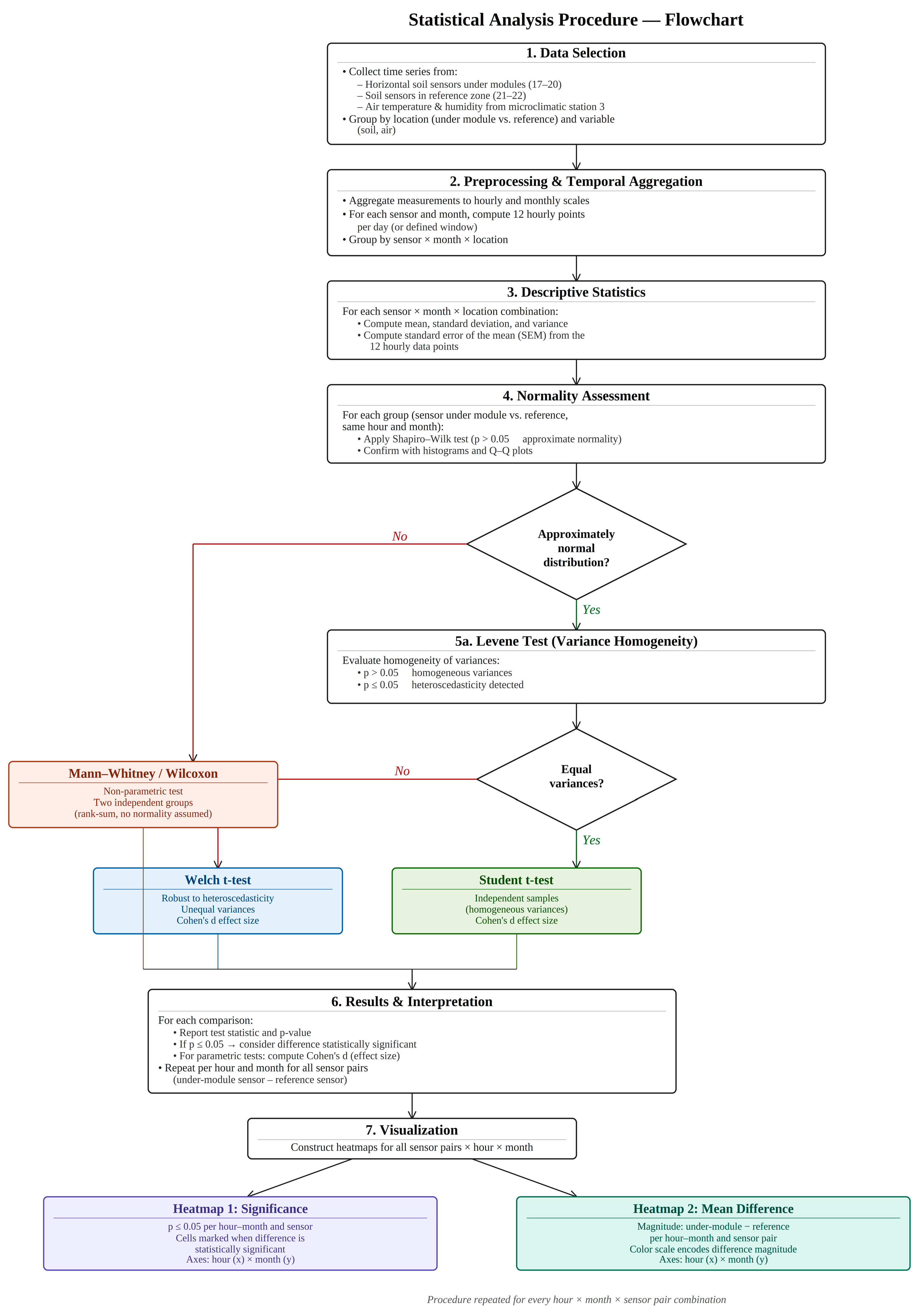
The analysis began with descriptive statistics—mean, standard deviation, and variance—to characterise the distribution of each sensor group. Prior to selecting between parametric and non-parametric inferential tests, normality was assessed for each group, as it is a prerequisite for valid univariate comparisons [25]. The Shapiro–Wilk test was applied (p > 0.05 taken as indicative of approximate normality), and results were corroborated by visual inspection of histograms and Q–Q plots. This combined approach is recommended because formal normality tests may lack statistical power in small samples while becoming excessively sensitive in large ones, making graphical diagnostics an essential complement [20].

Group comparisons were conducted using independent-samples t-tests where normality was deemed acceptable, and Wilcoxon rank-sum tests where it was not, following standard guidance that non-parametric alternatives provide robust inference when the normality assumption is violated [26]. For t-tests, variance homogeneity between groups was evaluated using Levene’s test. When Levene’s test yielded p > 0.05, the classical Student’s t-test was applied; when p ≤ 0.05, Welch’s t-test was used instead, as it maintains appropriate Type I error rates under heteroscedasticity with minimal loss of power when variances are equal [27].

For all statistically significant comparisons (p ≤ 0.05), Cohen’s d was calculated to quantify effect size and contextualise the practical relevance of observed differences. Reporting both significance and effect magnitude is consistent with current best-practice recommendations for statistical reporting in applied research [28].

To examine temporal patterns, sensor data were aggregated at hourly and monthly scales. For each horizontal sensor, independent-samples t-tests compared the hourly mean of each measuring point against the corresponding reference-area value. Statistical significance (p ≤ 0.05) was summarised in an hour-by-month heatmap, enabling straightforward identification of periods in which sensor readings differed systematically between locations. For each sensor–month combination, the mean and standard error of the mean (SEM) were derived from 12 measurement points per day. A second heatmap displayed the magnitude of mean differences (under-module minus reference) as a function of hour and month, providing a visual representation of both the direction and intensity of the agrivoltaic effect across the measurement period.

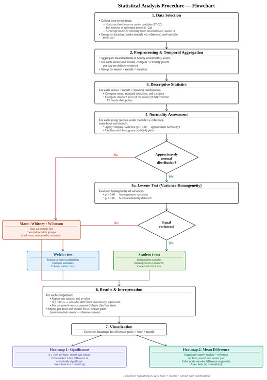
The complete analytical procedure, from data selection and preprocessing through inferential testing and visualisation, is summarised in Figure 4.

3. Results

3.1. Soil Moisture and Soil Temperature

In this first section, we present the soil sensor data, which gather soil moisture and soil temperatures simultaneously. Therefore, we present these results together.

3.1.1. Fourier Preprocessing

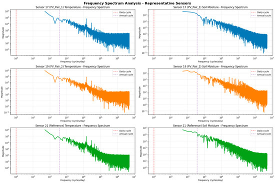
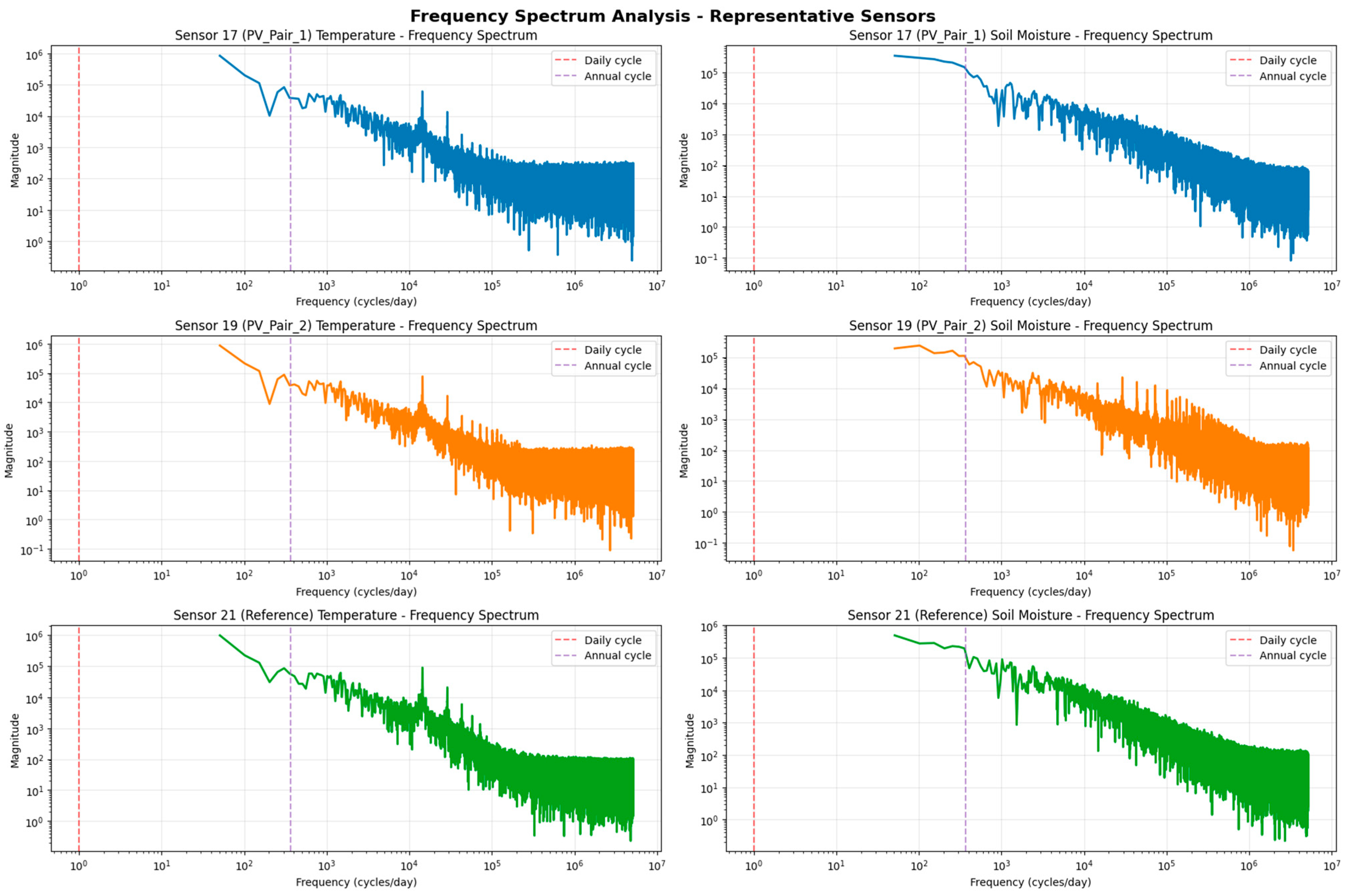
Figure 5 shows a comparative frequency domain analysis of temperature (left) and moisture (right) for three representative sensors: two located under PV modules (sensor 17—PV_Pair_1 and 19—PV_Pair_2), and one reference sensor (sensor 21) (not influenced by shading, Figure 1c). Each row corresponds to a sensor, with temperature spectra on the left and soil moisture spectra on the right. The vertical dashed lines show the expected daily (~1 cycle/day) and annual (~1/365 cycles/day) periodicities. The frequency spectrum analysis shows that, for all sensors and both temperature and soil moisture, variability is dominated by low frequencies, showing the prevalence of long-term and seasonal processes. Temperature exhibits clear daily and annual cycles, which are particularly pronounced under the PV modules, suggesting that PV modules enhance or modulate diurnal thermal forcing through altered radiative conditions, while the reference sensor displays smoother and less amplified behaviour. In contrast, soil moisture shows weaker but still identifiable periodicity, reflecting reduced sensitivity to diurnal forcing and stronger control by slower hydrological processes such as precipitation, drainage, and evapotranspiration. Across the spectra, PV sensors present higher magnitudes over a wider frequency range, especially at intermediate frequencies, which shows more complex short-to-medium timescale variability compared to the more stable reference conditions. At high frequencies, all signals converge toward a noise floor, consistent with the limited contribution of rapid fluctuations in environmental measurements.

The spectral analysis presented in Figure 5 yields the following specific conclusions in the context of this study. First, variability in both soil temperature and soil moisture is dominated by low-frequency components across all sensors, confirming that seasonal and long-term processes are the primary drivers of microclimate dynamics at the site. This is consistent with and provides a quantitative spectral basis for the seasonal patterns reported in the main results. Second, diurnal and annual periodicities in soil temperature are more pronounced beneath the PV modules than at the reference position, indicating that the panels do not simply attenuate thermal variability through shading but actively modulate the diurnal thermal cycle—likely through a combination of altered daytime radiative input via the 40% transmittance and modified nocturnal longwave dynamics beneath the glass surface. This finding nuances the interpretation of the mean temperature differentials reported elsewhere in the manuscript. Third, soil moisture spectra are spectrally flatter and show weaker periodicity than temperature spectra, reflecting the dominant control of episodic precipitation and slow hydrological processes over soil water dynamics, and explaining why moisture differences between zones are less temporally structured than temperature differences. Fourth, the broader spectral energy distribution of the under-panel sensors at intermediate frequencies indicates that the PV structure introduces additional complexity into the microclimate signal at short-to-medium timescales, consistent with the spatially and temporally heterogeneous radiative environment created by the panel array. Taken together, these spectral findings demonstrate that the agrivoltaic installation modifies not only the mean values of soil temperature and moisture but also the temporal structure of their variability—an insight that time-series analysis alone cannot provide.

3.1.2. Statistical Tests for Soil Moisture and Soil Temperature

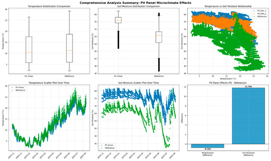
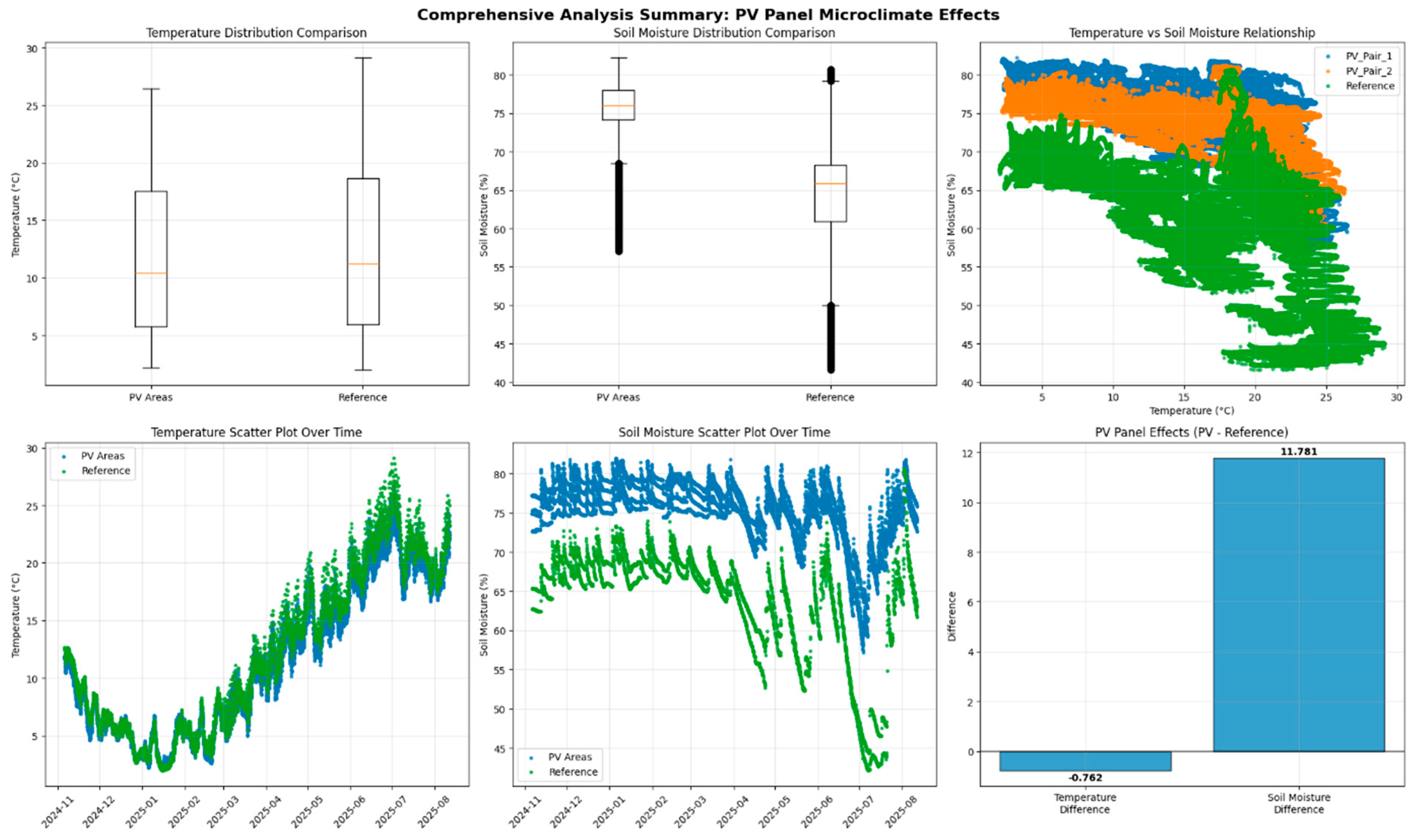
We performed a descriptive statistic, including mean, standard deviation, and effect size (Cohen’s d) to distinguish statistical from practical significance. The results are presented in Supplementary Material. The AV dataset shows small differences in soil temperature relative to the reference area. Mean soil temperature at AV sites is slightly lower (12 ± 6.4 °C; n ≈ 8.0 × 105) than in the reference area (12 ± 6.9 °C; n ≈ 4.0 × 105), corresponding to an average reduction of −0.76 °C. Although this difference is statistically detectable because of the very large sample size (p < 10⁻⁶), the associated effect size is small (Cohen’s d = −0.11), showing negligible practical relevance. From an applied perspective, soil temperatures at AV and reference sites can therefore be considered broadly comparable. Mean soil moisture at AV locations is 75 ± 3.9%, compared with 64 ± 7.0% in the reference sites, corresponding to an average increase of approximately 11%. This difference is not only statistically highly significant (p < 1.0 × 10⁻⁶) but also large in practical terms, as reflected by a very large effect size (Cohen’s d = 2.1). Such a high Cohen’s d-value shows a minimal overlap between the moisture distributions of the two areas, highlighting a pronounced and physically meaningful contrast in soil water conditions. To contextualise these effect sizes, we follow the conventional benchmarks proposed by Cohen [29], whereby d = 0.2 denotes a small effect, d = 0.5 a medium effect, and d ≥ 0.8 a large effect; values exceeding 2.0, as observed here for soil moisture, indicate a very large and practically important difference. Figure 6 illustrates these patterns: the box plots show lower and less variable temperatures under AV and substantially higher, more stable moisture; the time-series panels indicate that these differences persist throughout the year and intensify in summer. Overall, the results show modest cooling but a large, practically meaningful increase in soil moisture under AV, consistent with shading that reduces heating and evaporation.

The top-right panel (Figure 6) presents a box plot of soil temperature (°C), while the top-centre panel shows a box plot of soil moisture (%) showing the median, interquartile range, and whiskers. A relationship between temperature (°C) and soil moisture (%) is presented in Figure 6 in the top-left panel. The bottom-left and bottom-centre panels display time-series scatter plots for soil temperature and soil moisture, respectively, illustrating hourly observations together with monthly aggregated values. The bottom-right panel (Figure 6) summarises the AV–reference comparisons across sensors.

The six soil moisture sensors (SM17–SM22; with sensors 17, 18, 19 and 20 underneath the AV modules and sensors 21 and 22 in the reference area) reveal a clear seasonal cycle: high moisture in November–February, decreasing in March–May, and very low levels by July–August. While all sensors (Figure 6, bottom-centre panel) show minor timing or intensity differences, the overall pattern is consistent, with synchronous transitions suggesting a common environmental driver.

The soil temperature sensors display a clear pattern. They show a major seasonal transition from cool temperatures to hot temperatures. During the hotter period, the daily temperature cycle incorporates daytime peaks and cool nights. This pattern is an inversion of the soil moisture values, as rising temperatures correspond with a drop in soil moisture due to increased evaporation.

3.1.3. Comparison of Soil Moisture and Influence of Tree Distance

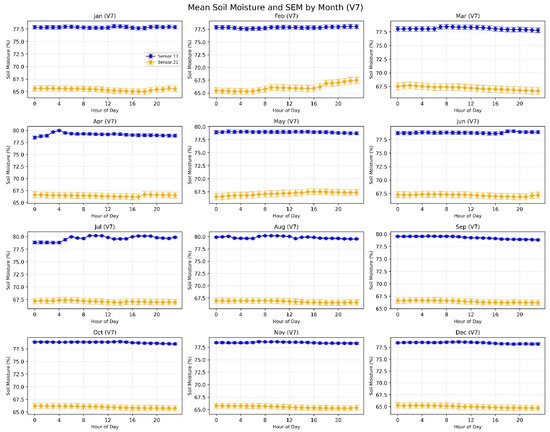
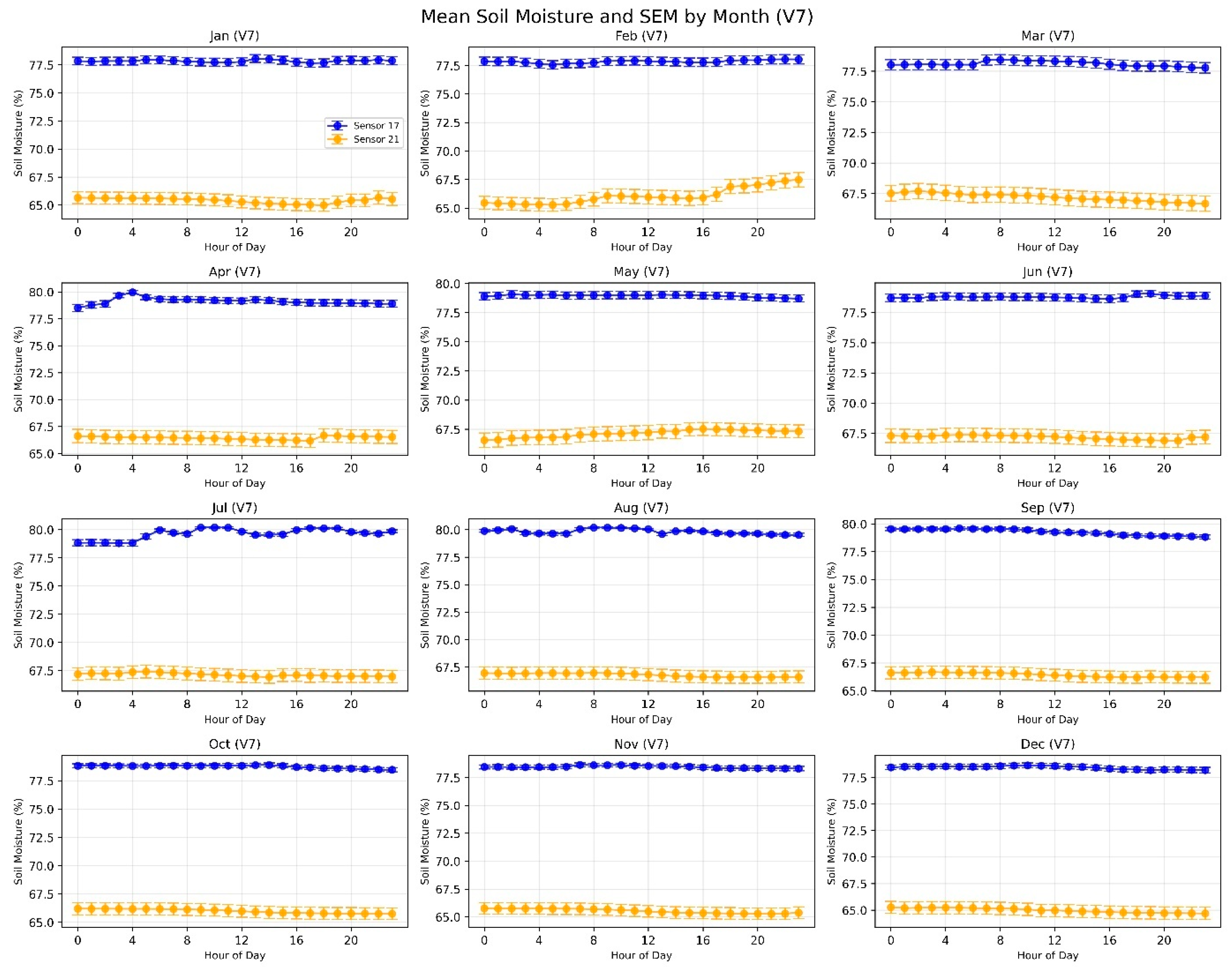
Independent-samples t-tests comparing drip-edge and reference values for each sensor (sensor 17 under the AV installation and sensor 21 in the reference area) consistently showed significant differences in soil moisture (p < 0.05). Monthly means and SEMs were also computed to characterise temporal variability. In total, twelve plots were produced, one for each sensor position at different distances from the trees (Figure 2b). Figure 7 presents the mean and standard error of the mean (SEM) for soil moisture measured by the V7 sensor at the drip edge beneath the AV modules (17). The distance between adjacent rows of apple trees is 3 m, with soil sensor 17 (channel 12) positioned at the midpoint between rows (Figure 2b). The sensor channels (1 to 12) are spaced at 10 cm intervals. Channel 1 is located 40 cm from the apple tree row, while channel 7 corresponds approximately to the drip line, which is located 1 m from the trees.

Comparisons of mean soil moisture (Figure 7) reveal consistently higher values at sensor 17 than at sensor 21, independent of month or dataset, indicating distinct microclimatic conditions. Neither sensor shows strong diurnal variation, suggesting limited influence of daily environmental cycles.

3.1.4. Comparison of Soil Temperature and the Influence of Tree Distance

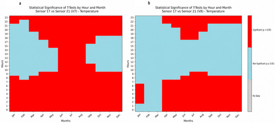
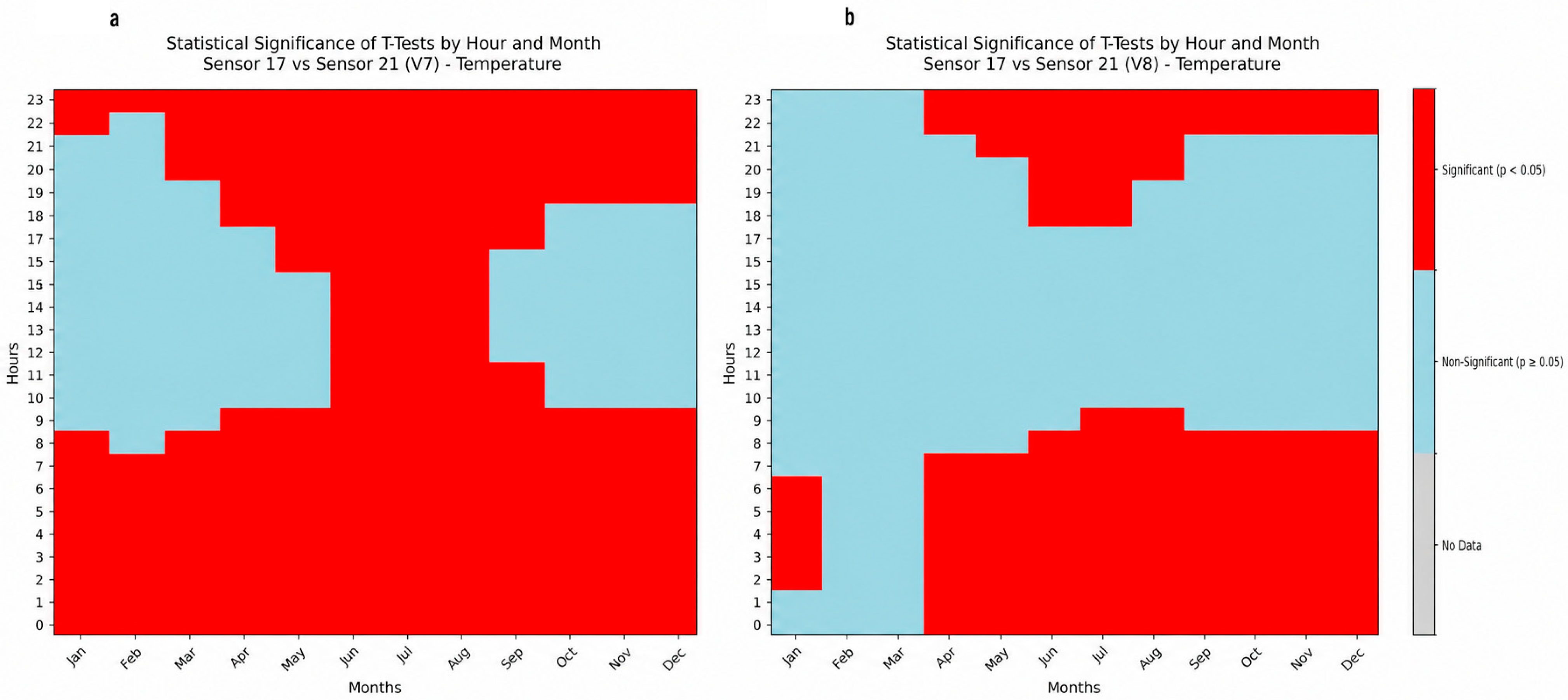
Normality was assessed with the Shapiro–Wilk test (p < 0.05 indicating deviation from normality). Subsequently, independent-samples t-tests were run for each hour and month across the 12 channels, comparing sensor 17 (located under PV modules) with sensor 21 (located in the reference area with no PV modules influencing the measurement). To move beyond binary significance testing, Cohen’s d was calculated for each hour–month combination to quantify the practical magnitude of observed differences, following the conventional Cohen benchmark (1988): d = 0.2 (small), d = 0.5 (medium), and d ≥ 0.8 (large). Figure 8 presents two heatmaps (in channels V7 and V8) comparing the soil temperature in these V7 and V8 soil temperature sensors. Red denotes significant differences (p < 0.05) with a meaningful effect size (Cohen’s d ≥ 0.2), and light blue non-significant results (p ≥ 0.05), thereby distinguishing cases where statistical significance reflects genuine practical relevance from those driven by large sample size alone. Significant contrasts with meaningful effect sizes recur across variants, especially in summer and during late afternoon to early evening, whereas several statistically significant results in transitional months show small effect sizes, suggesting limited practical importance despite their detectability.

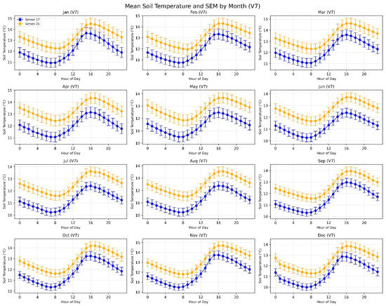
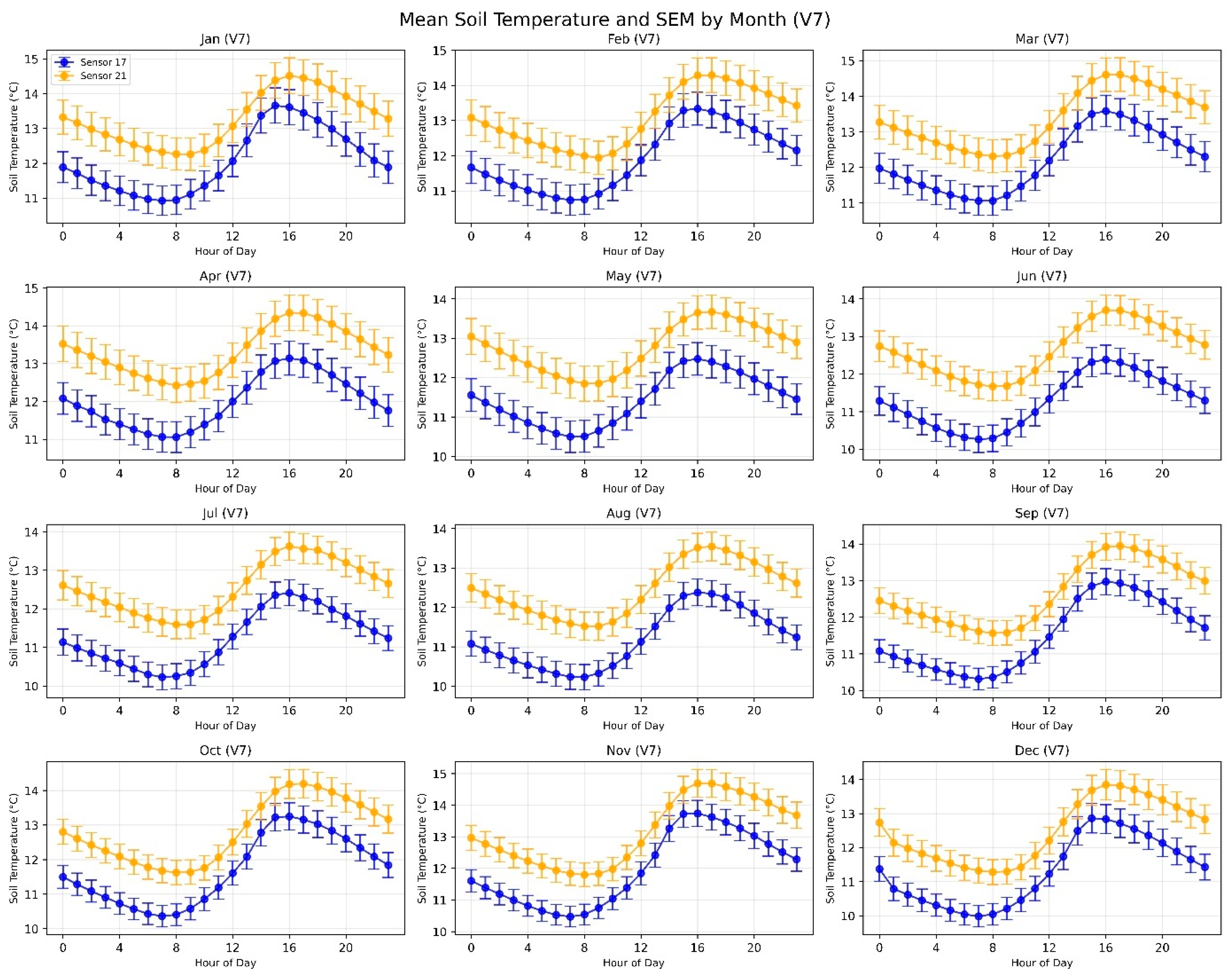
Figure 9 shows that sensor 17 generally records higher soil temperatures than sensor 21, showing a warmer microclimate at that location. Both sensors exhibit clear diurnal and seasonal cycles, with maxima in summer and minima in winter; amplitudes vary across data-collection periods. Small standard errors show precise mean estimates, while overlapping SEMs at night suggest that nocturnal differences are often not statistically distinguishable.

3.2. Air Temperature

3.2.1. Temporal Pattern Analysis for Air Temperature Sensors

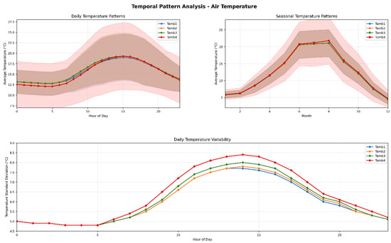
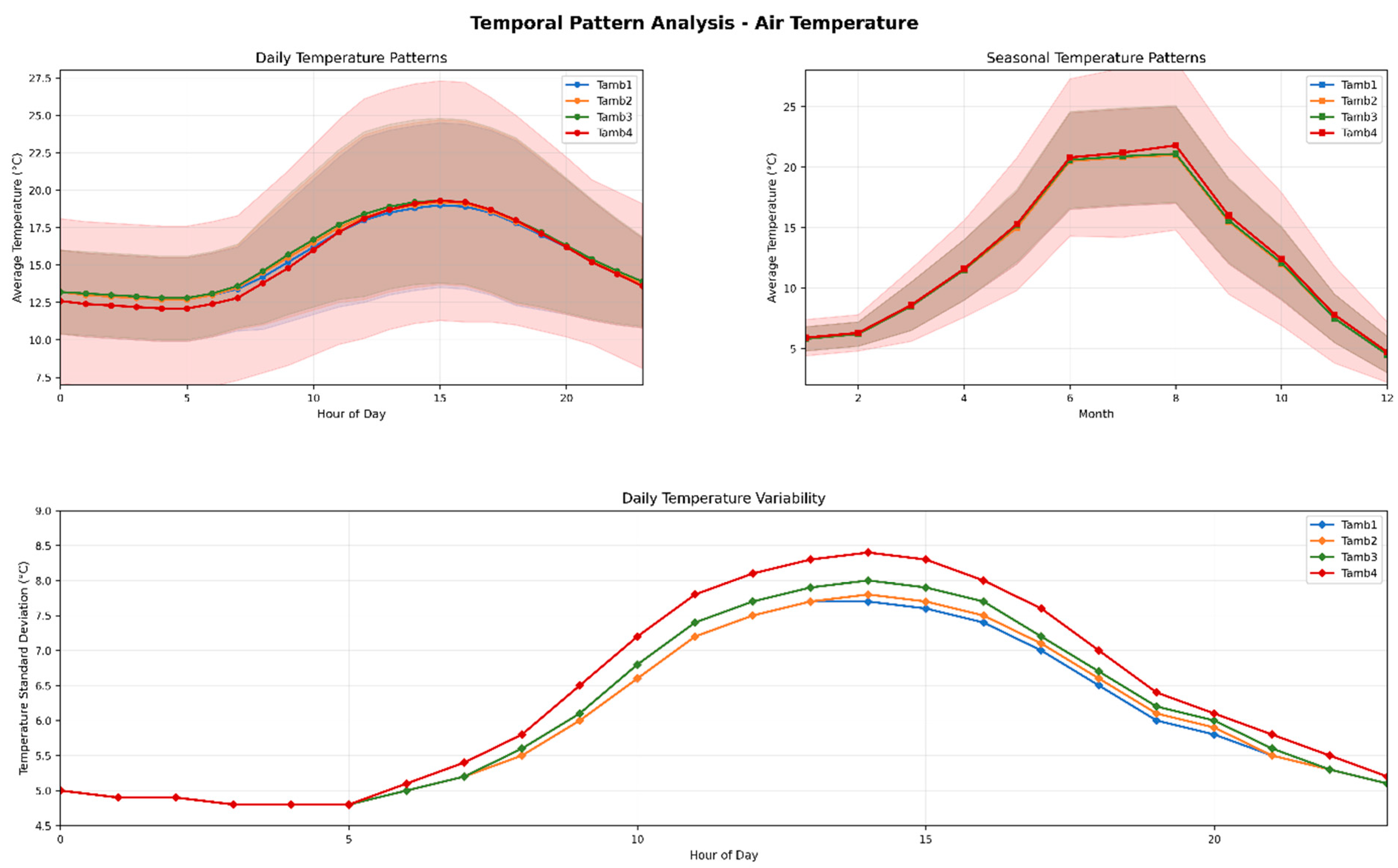
Figure 10 presents a comprehensive temporal analysis of air temperature data from four different locations, identified as Tamb1, Tamb2, Tamb3, and Tamb4, across four subplots (location and height of these sensors are shown in Table 1).

The top-left image displays the daily average temperature pattern and the top-right shows the seasonal temperature pattern. The shaded areas in both top panels represent the standard deviation, providing a visual sense of uncertainty or dispersion in the measurements. Temperatures follow a predictable pattern: they are lowest in the early morning and peak in the mid-afternoon, around 2 PM to 4 PM. Tamb4 consistently shows the highest temperatures, while Tamb1 and Tamb2 are the coolest, with Tamb3 falling in between. The bottom image presents daily temperature variability (standard deviation per hour). This metric shows how much the temperature fluctuates from its average for each hour of the day. Variability is lowest in the early morning and late evening and highest in the afternoon, which corresponds with the period of peak heating and cooling. All four locations exhibit a clear seasonal cycle, with the lowest temperatures occurring in the winter months (December to February) and the highest in the summer (June to August). Like the daily patterns, Tamb4 has the highest temperatures year-round, while the others are cooler.

3.2.2. Statistical Test for Air Temperature Sensors

The data from the ambient temperature sensors show a clear, consistent pattern. The four sensors are highly correlated, with coefficients of 0.99 or 1, showing they all capture the same overall temperature trends. Specifically, the time-series plot reveals a distinct seasonal cycle, with temperatures at their lowest in the winter months (e.g., January) and highest in the summer (e.g., July). While all sensors follow this trend, Tamb4 consistently records a slightly higher mean temperature (15.92 °C) and a wider spread of values compared to the others.

3.2.3. Influence of the Presence of PV Modules on Air Temperature

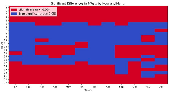
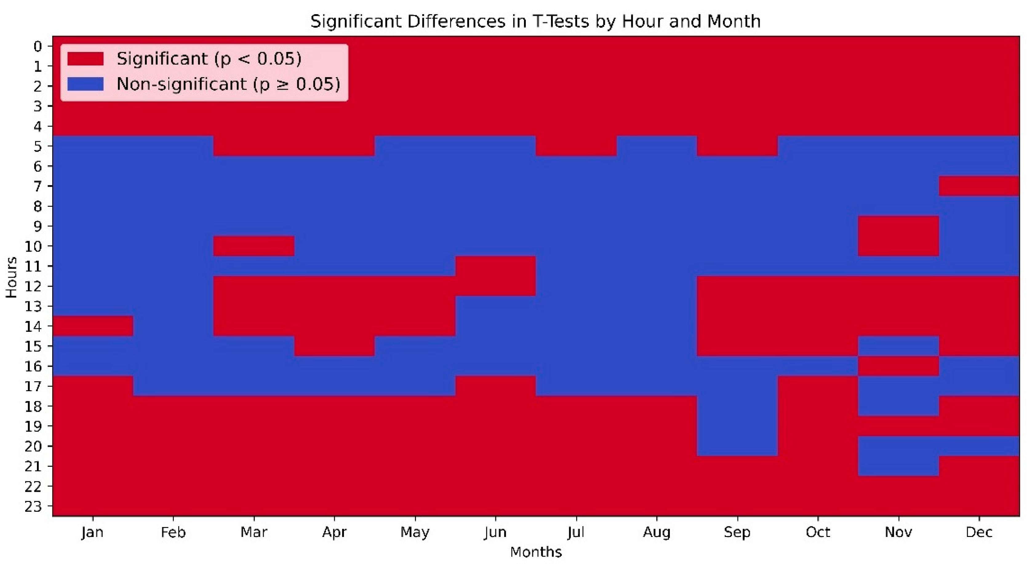
We analysed temperature data from two sensors, one under the PV modules (Tamb1) and one in an open-ceiling area (Tamb3), both at a height of 2 m. We performed hourly and monthly analyses, complemented by Cohen’s d calculations for each hour–month combination to assess practical significance alongside statistical significance, following the conventional benchmarks: d = 0.2 (small), d = 0.5 (medium), and d ≥ 0.8 (large). The t-test results, shown in Figure 11, indicate that red sections of the graph signify a statistically significant difference (p ≤ 0.05) with a meaningful effect size (Cohen’s d ≥ 0.2) and blue sections denote non-significant differences (p > 0.05), thereby distinguishing cases where statistical significance reflects genuine practical relevance from those driven by large sample size alone. This consistent difference is prominent from 16:00 to 23:00 year-round, and during midday (10:00 to 14:00) in spring and summer, where the effect sizes are largest, suggesting that the thermal buffering effect of the PV modules is not only statistically detectable but also physically meaningful during these periods. Conversely, the blue sections occur mostly from 0:00 to 6:00 and during midday in the fall and winter, where the absence of statistical significance is consistent with negligible effect sizes, indicating that temperature conditions under and outside the PV structure are practically equivalent during these periods.

When analysing the mean hourly temperature and SEM for sensors Tamb1 (under the PV modules) and Tamb3 (in an open-ceiling area) for each month, both sensors show a typical daily cycle with temperatures peaking in the afternoon and reaching their lowest point in the early morning. While the sensors track each other closely, a key difference is a consistent separation during the midday and afternoon (10:00 to 18:00), especially in spring and summer. During these times, Tamb3 consistently records a higher temperature than Tamb1. At night and in the early morning (20:00 to 8:00), the temperatures from both sensors are nearly identical. The larger error bars during the day indicate greater temperature variability during warmer hours.

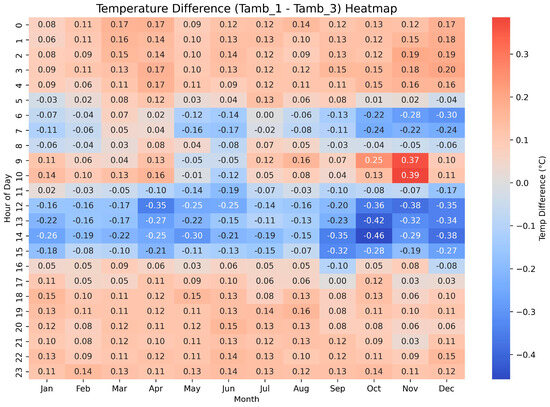
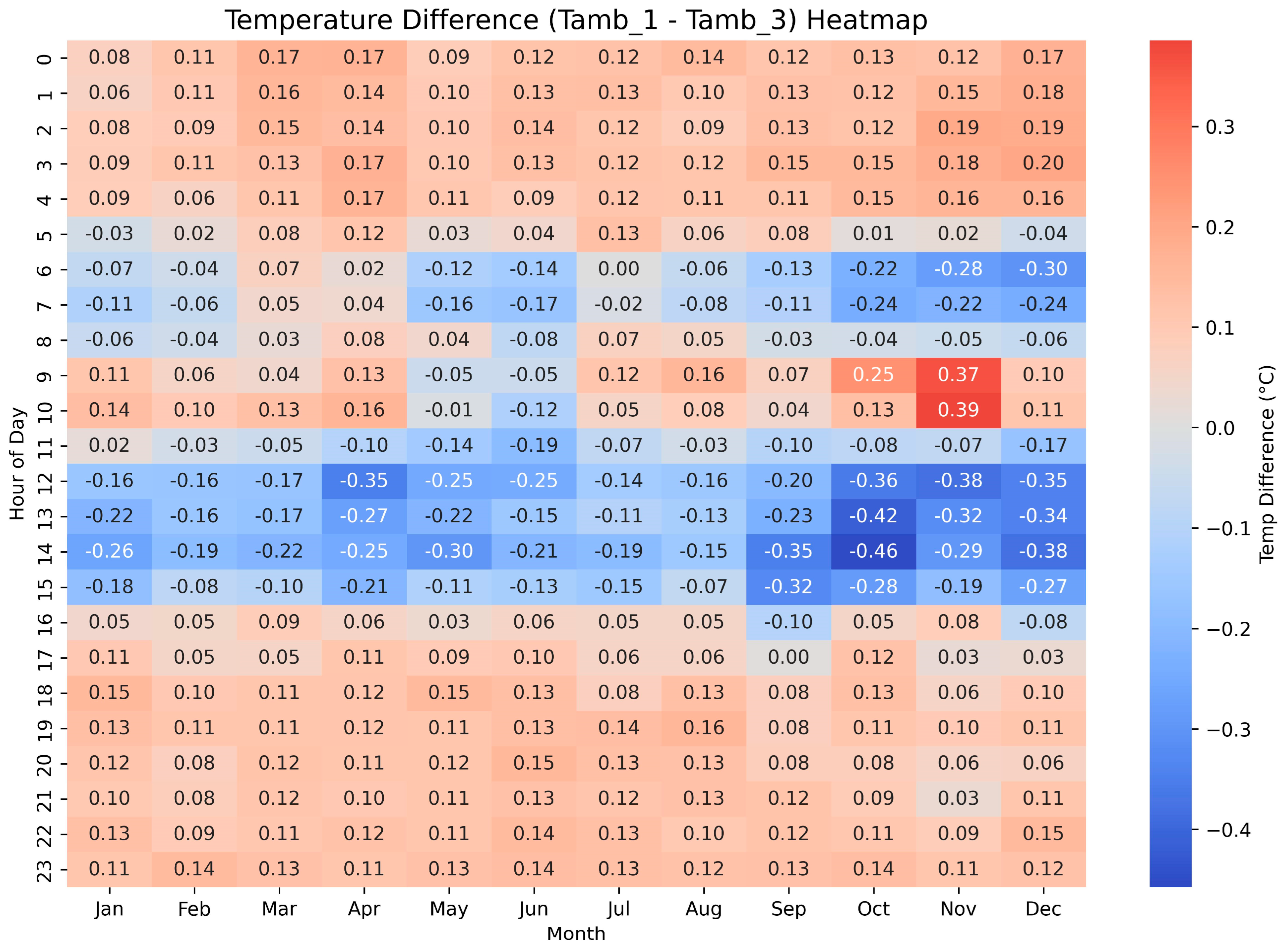
Figure 12 presents a heatmap of the hourly and monthly air temperature difference between a sensor beneath the PV modules (Tamb1) and a sensor in the open-ceiling area (Tamb3). Overall, Tamb1 is slightly warmer than Tamb3 during the late evening and early morning (18:00 to 09:00), with a temperature difference ranging from 0.05 to 0.17 °C. In contrast, during midday and the afternoon (10:00 to 17:00), the open-ceiling sensor (Tamb3) records higher temperatures than the sensor under the PV modules (Tamb1), particularly in spring and summer. The most pronounced negative differences, reaching up to −0.42 °C, occur in September and October.

3.3. Air Humidity

3.3.1. Sensor Comparison Analysis for Air Humidity Sensors

The analysis of air humidity data from three sensors (Relhumi1, Relhumi2, and Relhumi3) reveals they consistently measure similar trends, despite the data’s inherent daily and seasonal fluctuations. While Relhumi1 has a slightly higher median, all three sensors exhibit similar distributions and a wide range of extreme values. This consistency is strongly supported by a correlation matrix, which shows a very strong positive correlation (minimum of 0.98) among all sensors. In conclusion, although air humidity levels are variable, the sensors provide consistent and accurate measurements of the same patterns.

3.3.2. Temporal Pattern Analysis for Air Humidity Sensors

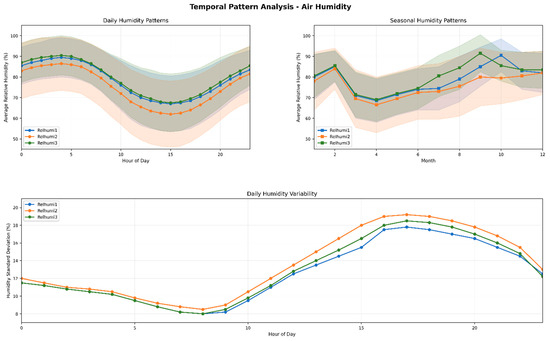
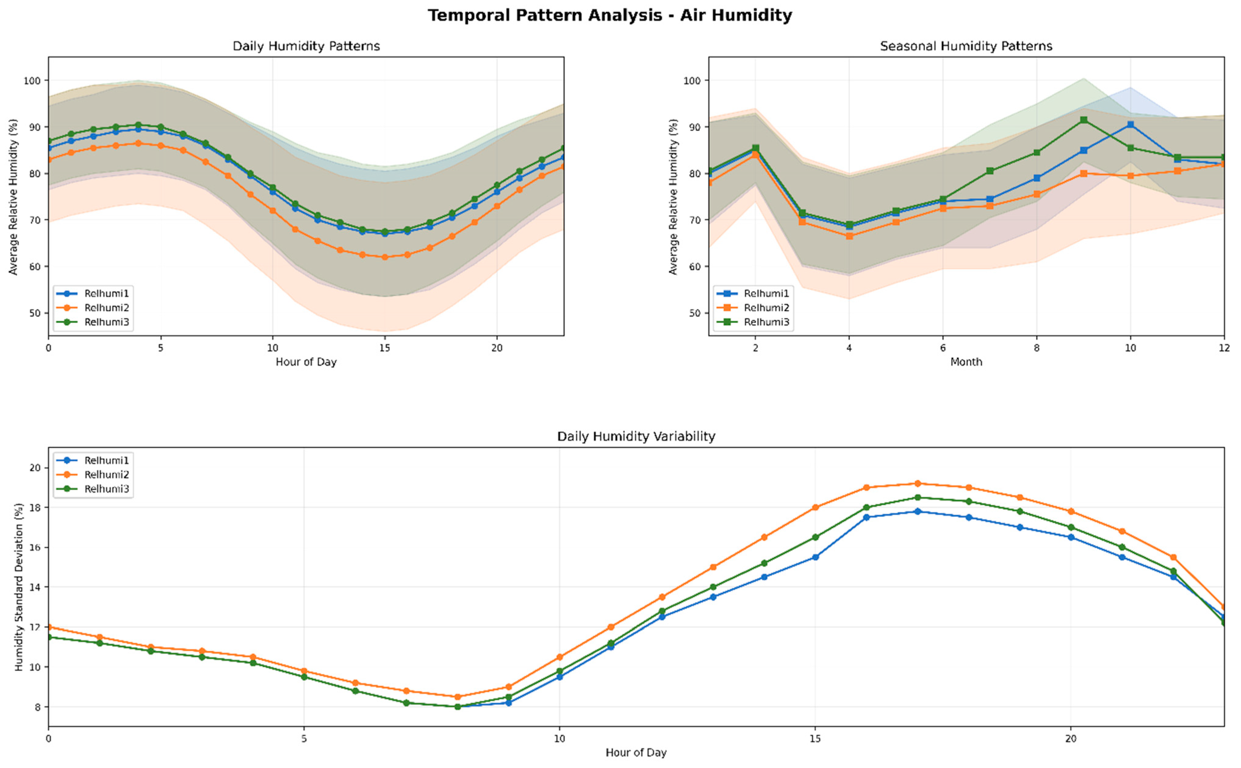
Based on the analysis of Figure 13, the daily humidity chart shows a clear inverse relationship with temperature, with humidity highest in the early morning and lowest in the mid-afternoon. There is a distinct seasonal trend, with the highest humidity levels occurring during the summer and autumn months (June to October) and the lowest in the spring (March to May). The data also reveal that humidity is most stable with the lowest variability in the early morning. In contrast, the afternoon hours, particularly from 3 PM to 5 PM, are a period of higher humidity fluctuation and instability. Notably, the Relhumi3 sensor exhibits slightly higher daily variability than the others.

3.3.3. Statistical Test for Air Humidity Sensors

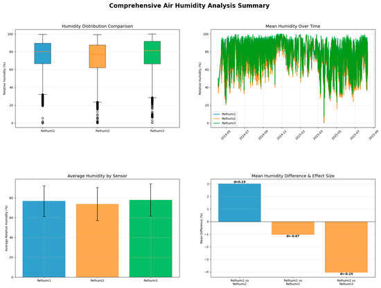
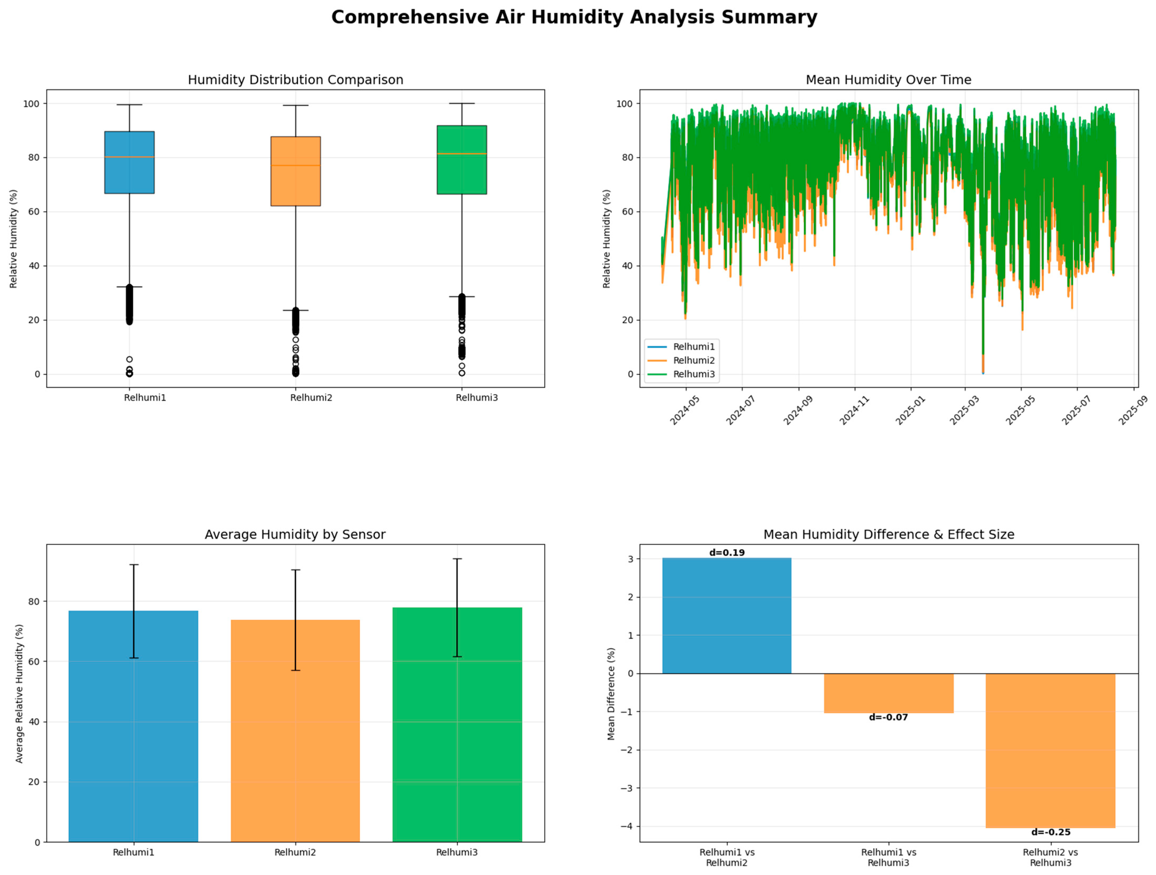
Based on the analysis of Figure 14, all three humidity sensors show statistically significant differences, a result likely influenced by the very large sample size of over 440,000 data points. While the differences are statistically significant (p < 10⁻⁶), the effect sizes (Cohen’s d) for the comparisons between Relhumi1, Relhumi2, and Relhumi3 are negligible or very small. This suggests that while the differences are not due to random chance, they may not be practically meaningful in real-world contexts.

3.3.4. Influence of the Presence of PV Modules on Air Humidity—Under PV and Open Ceiling

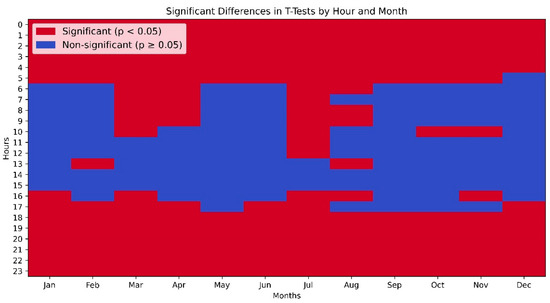
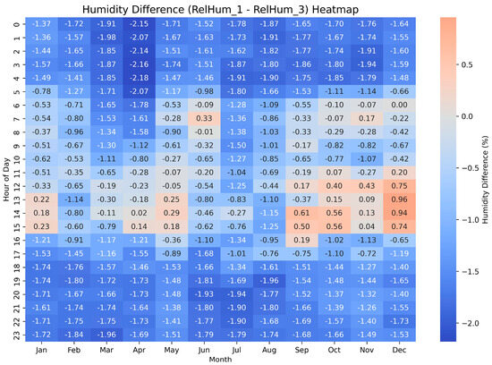
Figure 15 and Figure 16 compare humidity from RelHum1 (sensor located under PV) and RelHum3 (sensor located in open air in the reference area). Both follow the expected cycle—highest at night/early morning, lowest midday/afternoon. While the mean relative humidity difference offers a useful aggregate measure, it obscures a pronounced diurnal asymmetry, with systematically different patterns between daytime and nighttime conditions that are critical for interpreting the observed microclimate.

To distinguish statistically detectable differences from practically meaningful ones, Cohen’s d was calculated for each hour–month combination alongside the t-test results, following the conventional benchmarks. Figure 15 adopts the same colour scheme applied throughout this study: red denotes statistically significant differences with a meaningful effect size (p < 0.05), and blue denotes non-significant results (p ≥ 0.05). Statistically significant differences (p < 0.05) occur mainly from 16:00 to 06:00, when RelHum1 is consistently higher than RelHum3, especially in spring and summer; effect sizes during these periods are largest, indicating that the humidity contrast beneath the PV structure is not only statistically detectable but also physically meaningful. During the day, from 11:00 to 15:00, values converge and effect sizes diminish markedly, with RelHum3 being slightly higher than RelHum1 in autumn and winter, a pattern that is statistically significant in some months but of negligible practical magnitude. Overall, humidity differences consistently reverse between night and day, with the most practically relevant contrasts concentrated in the evening and nocturnal hours during the warmer months.

4. Discussion

This study is based on a single 12-month monitoring period (August 2024–August 2025) and should be interpreted accordingly. While the relative microclimatic differences between under-panel and open-field zones are robust, their absolute magnitude likely depends on interannual climate variability. Hot, dry years may enhance the cooling and soil moisture retention effects of the panels, whereas cooler, wetter conditions may diminish them. The attenuation of temperature extremes may be especially relevant during heatwaves. Thus, these results provide a context-specific assessment, and multi-year monitoring is needed to evaluate the stability and climatic sensitivity of the observed effects. This study shows that AV systems substantially modify orchard microclimates, with predominantly beneficial effects for apple production. This discussion section focuses on the four parameters analysed in this work, and we highlight the results achieved by other approaches in Table 2.

Soil moisture increased by 11.78% under the semi-transparent PV modules, indicating improved water retention and reduced irrigation demand. This result falls within the range reported for irrigated vegetable systems in arid environments (5–15%, Barron-Gafford et al., 2019 [11]). In contrast, some studies have documented increases of up to 100% in specific locations [30]; however, these larger effects appear to be highly site-specific and are primarily associated with rainfall redistribution at the panel edges. Other authors have reported a 10–40% reduction in evapotranspiration under similar conditions (Marrou et al., 2013 [17]), which is consistent with higher soil moisture content.

Across climates and system designs, AV/PV shading consistently reduces soil temperature by ~0.5–2.3 °C (Marrou et al., 2013 [17]), with magnitude depending on crop, depth, panel density, and season. We observed that the average reduction (−0.76 °C) sits comfortably within this reported range, aligning closely with irrigated vegetable contexts (≈−0.5 to −1 °C) and a bit below the stronger cooling seen in cereals at depth (≈−2 °C) [31]. This aligns with previous findings, indicating that the AV installation in Kressbronn provides a measurable cooling effect on the soil, thereby buffering root-zone temperatures against thermal extremes.

Similarly, air temperatures beneath the modules were slightly higher in the early morning (+0.2 °C) but lower at midday (−0.5 °C), indicating moderation of thermal extremes. Such regulation may help mitigate crop stress during periods of high radiation. Several studies have documented the cooling effects of AV systems on microclimatic conditions, particularly temperature. For example, ref. [11] reported that air temperatures beneath photovoltaic (PV) panels in a semi-arid region of Arizona were approximately 2–3 °C lower during the daytime compared to unshaded control plots. The smaller air temperature reduction observed here (−0.5 °C vs. 2–3 °C in [11]) is explained by contextual and design differences rather than contradiction. The Kressbronn site’s temperate, humid climate with lower irradiance limits shading-induced cooling compared to the semi-arid, high-radiation environment of Tucson. Additionally, semi-transparent PV panels (≈40% transmission) reduce the net radiative blocking relative to opaque systems. Higher panel mounting and stronger wind-driven mixing near Lake Constance further enhance ventilation and diminish thermal contrasts. Together, these factors coherently explain the weaker cooling effect observed.

AV creates microclimatic conditions that increase relative humidity beneath the panels. A key driver of this shift is the reduction in solar irradiance and ventilation caused by wind obstruction from the panels, which in turn lowers both air and soil temperatures. As a result, evaporation of soil moisture and plant transpiration rates decline. Relative air humidity was reduced in our work by 2.16%. While lower humidity may increase evaporative demand in dry climates, in temperate regions such as southern Germany it is likely advantageous, as it reduces the risk of fungal diseases in apples. Higher results were achieved by Weselek et al. (2021) [29], who documented RH increases between 5 and 10% during summer trials in German orchards. Further studies by [17,32] revealed that daily mean air humidity under PV panels was consistently ~2% higher over several months. Humidity is the primary climatic driver of fungal disease outbreaks globally, associated with 36.4% of reported cases, and elevated moisture broadly enhances pathogen germination, infection, and survival across foliar and fruit diseases [33,34]. Agrivoltaic structures may partially mitigate this risk by intercepting rain splash—with documented benefits in mango and grape—though their typically incomplete field coverage means the net effect on disease incidence under agrivoltaic conditions remains uncertain [35].

Table 2. Comparison of climatic variations caused by AV installations.

	Study & Location	Climate K-G	Crop/System	Soil Temperature Change Under AV
Soil Temperature	[28], Herwangen-Schönach, Ger.	Cfb	Mixed crops under elevated AV	−1.2 °C (2017 mean daily), −1.4 °C (2018 mean daily); cooler from March–mid-Oct on most days
	[26], Montpellier, France	Csa	Lettuce, wheat	−0.5 °C (irrigated lettuce); −2.3 °C (25 cm) and −1.9 °C (5 cm) in wheat; cooler under shade; effect varies with module density
	[32], Fort Collins, CO, USA	BSk	Summer squash, peppers, tomatoes, and lettuce	5.8 °C, under bifacial PV 9 °C under semi-transparent PV 14.4 °C opaque silicon
	Kressbronn Germany	Cfb	Apple orchard (semi-transparent PV, 40% transmittance)	−0.76 °C (mean value)
	[27], Wiltshire, UK	Cfb	Grassland	4 °C cooler under panels vs. gaps between rows
Soil Moisture	Barron-Gafford et al. (2019) [11], (Tucson, AZ, USA)	Bwh	Dryland vegetables	+15% vs. open field
				+5% vs. open field
	Hassanpour et al., (2018) [20] (USA)	Csb	Unirrigated pasture	Localised zones beneath panels showed ≈100% higher soil moisture compared to adjacent plots
	Marrou, Dufour & Wéry (2013) [17] (Montpellier, France)	Csa	Lettuce (experimental)	10–30% lower evapotranspiration, implying higher water retention
	Kressbronn Germany	Csb	Apple orchard (semi-transparent PV, 40% transmittance)	+11.78% average soil moisture beneath PV modules compared to open reference
Air Temperature	[11], (Tucson, AZ, USA)	Bwh	Dryland vegetables	1.2 ± 0.3 (daytime average)
	[36], Mellemort, France	Csa	Golden Delicious apple	3.8 (with tracking panels)
	[31]	Review paper		1–4 (general range)
	[28], Herwangen-Schönach,	Cfb	Mixed crops under elevated AV	Reduction observed
	[32], Massachusetts, United States.	DFa	Cranberry plants	1–4 (general range)
	[31], Wiltshire, United Kingdom	Cfb	Grassland	2 °C cooler under panels vs. gaps between rows
	[33], Tsukuba, Japan	Cfa	Rice	0.8 °C
	[29]	Model	-	10 °C in soyabeans
	Kressbronn, (this study)	Csb	Apple orchard (semi-transparent PV, 40% transmittance)	−0.5 °C (mean value)
Relative Humidity	[29], Herwangen-Schönach, Germany	Cfb	Mixed crops under elevated AV	5–10%, no significant difference, slight reduction in RH
	[37] Singapore	Review paper		Lower RH on sunny days compared to cloudy days under the AV system
	Kressbronn	Cfb	Apple orchard (semi-transparent PV, 40% transmittance)	2.16% (mean value)
	[17]	Csa	Lettuce, wheat	~2% higher
	[36], Mellemort, France	Csa	Golden Delicious apple	+14% under shading conditions

Table 2. Comparison of climatic variations caused by AV installations.

	Study & Location	Climate K-G	Crop/System	Soil Temperature Change Under AV
Soil Temperature	[28], Herwangen-Schönach, Ger.	Cfb	Mixed crops under elevated AV	−1.2 °C (2017 mean daily), −1.4 °C (2018 mean daily); cooler from March–mid-Oct on most days
	[26], Montpellier, France	Csa	Lettuce, wheat	−0.5 °C (irrigated lettuce); −2.3 °C (25 cm) and −1.9 °C (5 cm) in wheat; cooler under shade; effect varies with module density
	[32], Fort Collins, CO, USA	BSk	Summer squash, peppers, tomatoes, and lettuce	5.8 °C, under bifacial PV 9 °C under semi-transparent PV 14.4 °C opaque silicon
	Kressbronn Germany	Cfb	Apple orchard (semi-transparent PV, 40% transmittance)	−0.76 °C (mean value)
	[27], Wiltshire, UK	Cfb	Grassland	4 °C cooler under panels vs. gaps between rows
Soil Moisture	Barron-Gafford et al. (2019) [11], (Tucson, AZ, USA)	Bwh	Dryland vegetables	+15% vs. open field
				+5% vs. open field
	Hassanpour et al., (2018) [20] (USA)	Csb	Unirrigated pasture	Localised zones beneath panels showed ≈100% higher soil moisture compared to adjacent plots
	Marrou, Dufour & Wéry (2013) [17] (Montpellier, France)	Csa	Lettuce (experimental)	10–30% lower evapotranspiration, implying higher water retention
	Kressbronn Germany	Csb	Apple orchard (semi-transparent PV, 40% transmittance)	+11.78% average soil moisture beneath PV modules compared to open reference
Air Temperature	[11], (Tucson, AZ, USA)	Bwh	Dryland vegetables	1.2 ± 0.3 (daytime average)
	[36], Mellemort, France	Csa	Golden Delicious apple	3.8 (with tracking panels)
	[31]	Review paper		1–4 (general range)
	[28], Herwangen-Schönach,	Cfb	Mixed crops under elevated AV	Reduction observed
	[32], Massachusetts, United States.	DFa	Cranberry plants	1–4 (general range)
	[31], Wiltshire, United Kingdom	Cfb	Grassland	2 °C cooler under panels vs. gaps between rows
	[33], Tsukuba, Japan	Cfa	Rice	0.8 °C
	[29]	Model	-	10 °C in soyabeans
	Kressbronn, (this study)	Csb	Apple orchard (semi-transparent PV, 40% transmittance)	−0.5 °C (mean value)
Relative Humidity	[29], Herwangen-Schönach, Germany	Cfb	Mixed crops under elevated AV	5–10%, no significant difference, slight reduction in RH
	[37] Singapore	Review paper		Lower RH on sunny days compared to cloudy days under the AV system
	Kressbronn	Cfb	Apple orchard (semi-transparent PV, 40% transmittance)	2.16% (mean value)
	[17]	Csa	Lettuce, wheat	~2% higher
	[36], Mellemort, France	Csa	Golden Delicious apple	+14% under shading conditions

Beyond the microclimatic characterisation presented in this study, the increase in soil moisture observed beneath the PV modules has potentially important agronomic implications for apple orchard management. Soil water availability is a key driver of apple productivity across several critical phenological stages. During flowering and fruit set, adequate soil moisture supports cell division and early fruit development, whereas water deficits at these stages reduce both fruit number and size [37]. During the fruit expansion period, sustained water availability promotes cell enlargement and is positively associated with fruit weight, firmness and sugar accumulation [38]. Consistently higher soil moisture under the modules compared with the reference area suggests that AV shading may lower evapotranspiration and enhance water retention in the upper soil profile, thereby reducing irrigation requirements and buffering short-term drought stress. Similar water-conserving effects have been reported for mulching and shading strategies in apple orchards and other perennial systems, which improved soil water status, increased yields, and enhanced water productivity by reducing soil evaporation [20,39].

However, although the present experiment spans a full annual cycle, it still represents a single-year observation and therefore may not capture the interannual variability in the seasonal dynamics of apple development. It remains unclear whether the soil moisture differences documented here would persist across multiple years and variable climatic conditions, and whether they consistently translate into measurable changes in yield, fruit quality, or harvest timing [40].

Future research should adopt an integrated, multi-year approach that combines phenological monitoring, tree water status, and fruit quality assessments with continuous microclimate and soil moisture measurements across several growing seasons. This would enable a more robust evaluation of the agronomic significance of the conditions observed beneath the PV modules and provide clearer insight into the suitability of agrivoltaic systems for apple production. Such long-term data would also help identify design and management strategies capable of balancing energy generation with consistent yields and fruit quality.

Beyond temporal depth, future studies should strengthen their spatial design by incorporating replicated measurement points and, where feasible, pre-installation baseline data to support stronger causal inference. At the within-installation scale, the present study characterised mean microclimate conditions across three functional zones—sub-panel, drip edge, and open interrow—but did not resolve fine-scale lateral gradients in soil moisture and temperature with distance from the panel edge. Addressing this gap will require higher-density sensor arrays deployed along cross-panel transects, which would enable dedicated spatial heterogeneity analyses and substantially advance understanding of the microhydrological and thermal redistribution processes that govern agrivoltaic system behaviour.

5. Conclusions

This study demonstrates that elevated agrivoltaic (AV) systems generate a measurable and agronomically relevant microclimatic improvement in orchards. The key findings can be summarised as follows:

• Soil moisture increased by 11.8% beneath the PV modules, due to reduced evapotranspiration and greater water retention, with clear edge effects at module boundaries reflecting spatial gradients in water availability. This suggests that the geometric design and arrangement of the modules spatially influence water availability in the surface soil profile.
• Soil temperature was moderately reduced (−0.8 °C on average), resulting in a more stable thermal regime beneficial for root and microbial activity.
• Agrivoltaic systems induced a notable buffering effect on air temperature, with slight warming at dawn (+0.2 °C) and moderate cooling at midday (−0.5 °C), reducing daily thermal extremes and associated crop heat stress. Relative humidity decreased by 2.16% beneath the panels—a counterintuitive outcome given the cooler conditions, but explained by the suppression of soil evaporative flux: solar panels retained soil moisture rather than allowing it to be released as vapour, so the reduction in atmospheric water content outweighed the thermodynamic tendency toward higher humidity under cooler air. This net reduction in humidity is a particularly relevant finding for disease management, as humidity is the primary climatic driver of fungal outbreaks, and even moderate decreases can reduce pathogen germination, infection efficiency, and survival. In high-humidity temperate orchards—such as apple-growing regions in the Lake Constance area of Germany, where humidity-driven diseases such as apple scab and powdery mildew pose persistent agronomic challenges—agrivoltaic-induced humidity reduction may therefore represent a meaningful and underexplored co-benefit of these dual land-use systems, warranting targeted investigation in future long-term and multi-site studies.
• Drip edge effects were confirmed, with the drip line exhibiting a distinct microclimate intermediate between the panel interior and fully exposed areas: locally higher soil moisture due to runoff concentration, combined with a thermal regime closer to uncovered conditions given the reduced overhead cover. These well-defined edge effects have relevant implications for root development and the spatial distribution of crop vigour.

Overall, these results support the use of AV installations not only as a renewable energy source, but also as a microclimatic management tool to enhance orchard resilience and sustainability. Future research should focus on long-term crop yield responses under AV systems, the optimisation of module geometry for different orchard configurations, and the evaluation of these microclimatic effects across diverse climatic regions.

References

- Energy, S.P. Technology Roadmap; IEA: Paris, France, 2014. [Google Scholar]
- Pardo, M.A.; Navarro-González, F.J. Sizing and Scheduling Optimisation Method for Off-Grid Battery Photovoltaic Irrigation Networks. Renew. Energy 2024, 221, 119822. [Google Scholar] [CrossRef] [Scilit]
- Pascaris, A.S.; Schelly, C.; Burnham, L.; Pearce, J.M. Integrating Solar Energy with Agriculture: Industry Perspectives on the Market, Community, and Socio-Political Dimensions of Agrivoltaics. Energy Res. Soc. Sci. 2021, 75, 102023. [Google Scholar] [CrossRef] [Scilit]
- Mamun, M.A.A.; Dargusch, P.; Wadley, D.; Zulkarnain, N.A.; Aziz, A.A. A Review of Research on Agrivoltaic Systems. Renew. Sustain. Energy Rev. 2022, 161, 112351. [Google Scholar] [CrossRef] [Scilit]
- Dinesh, H.; Pearce, J.M. The Potential of Agrivoltaic Systems. Renew. Sustain. Energy Rev. 2016, 54, 299–308. [Google Scholar] [CrossRef] [Scilit]
- Campana, P.E.; Stridh, B.; Amaducci, S.; Colauzzi, M. Optimisation of Vertically Mounted Agrivoltaic Systems. J. Clean. Prod. 2021, 325, 129091. [Google Scholar] [CrossRef] [Scilit]
- Taylor, M.; Pettit, J.; Sekiyama, T.; Sokołowski, M.M. Justice-Driven Agrivoltaics: Facilitating Agrivoltaics Embedded in Energy Justice. Renew. Sustain. Energy Rev. 2023, 188, 113815. [Google Scholar] [CrossRef] [Scilit]
- Biró-Varga, K.; Sirnik, I.; Stremke, S. Landscape User Experiences of Interspace and Overhead Agrivoltaics: A Comparative Analysis of Two Novel Types of Solar Landscapes in the Netherlands. Energy Res. Soc. Sci. 2024, 109, 103408. [Google Scholar] [CrossRef] [Scilit]
- Hayibo, K.S.; Pearce, J.M. Vertical Free-Swinging Photovoltaic Racking Energy Modeling: A Novel Approach to Agrivoltaics. Renew. Energy 2023, 218, 119343. [Google Scholar] [CrossRef] [Scilit]
- Zhang, L.; Gong, J.; Yang, Z.; Wu, X.; Wang, W.; Yang, C.; Xu, G.; Wu, C.; Bao, E. Evaluating the Contribution of Decreasing Heights of Photovoltaic Panels on Light Environment and Agricultural Production in Agrivoltaic Systems. J. Clean. Prod. 2025, 495, 145091. [Google Scholar] [CrossRef] [Scilit]
- Barron-Gafford, G.A.; Pavao-Zuckerman, M.A.; Minor, R.L.; Sutter, L.F.; Barnett-Moreno, I.; Blackett, D.T.; Thompson, M.; Dimond, K.; Gerlak, A.K.; Nabhan, G.P.; et al. Agrivoltaics Provide Mutual Benefits across the Food–Energy–Water Nexus in Drylands. Nat. Sustain. 2019, 2, 848–855. [Google Scholar] [CrossRef] [Scilit]
- Zainali, S.; Ma Lu, S.; Stridh, B.; Avelin, A.; Amaducci, S.; Colauzzi, M.; Campana, P.E. Direct and Diffuse Shading Factors Modelling for the Most Representative Agrivoltaic System Layouts. Appl. Energy 2023, 339, 120981. [Google Scholar] [CrossRef] [Scilit]
- Touil, S.; Richa, A.; Fizir, M.; Bingwa, B. Shading Effect of Photovoltaic Panels on Horticulture Crops Production: A Mini Review. Rev. Environ. Sci. Biotechnol. 2021, 20, 281–296. [Google Scholar] [CrossRef] [Scilit]
- Laub, M.; Pataczek, L.; Feuerbacher, A.; Zikeli, S.; Högy, P. Contrasting Yield Responses at Varying Levels of Shade Suggest Different Suitability of Crops for Dual Land-Use Systems: A Meta-Analysis. Agron. Sustain. Dev. 2022, 42, 51. [Google Scholar] [CrossRef] [Scilit]
- Vélez, S.; Bretzel, T.; Pöter, R.; Berwind, M.F.; Trommsdorff, M. IoT-Based Monitoring of Overhead Agrivoltaic 2 Systems to Analyze the Delay in Apple Ripening and 3 Its Influence on Maturation Patterns. 2025. Available online: https://papers.ssrn.com/sol3/papers.cfm?abstract_id=5102506 (accessed on 3 March 2026).
- Yavari, R.; Zaliwciw, D.; Cibin, R.; McPhillips, L. Minimizing Environmental Impacts of Solar Farms: A Review of Current Science on Landscape Hydrology and Guidance on Stormwater Management. Environ. Res. Infrastruct. Sustain. 2022, 2, 032002. [Google Scholar] [CrossRef] [Scilit]
- Marrou, H.; Guilioni, L.; Dufour, L.; Dupraz, C.; Wery, J. Microclimate under Agrivoltaic Systems: Is Crop Growth Rate Affected in the Partial Shade of Solar Panels? Agric. For. Meteorol. 2013, 177, 117–132. [Google Scholar] [CrossRef] [Scilit]
- Choi, C.S.; Cagle, A.E.; Macknick, J.; Bloom, D.E.; Caplan, J.S.; Ravi, S. Effects of Revegetation on Soil Physical and Chemical Properties in Solar Photovoltaic Infrastructure. Front. Environ. Sci. 2020, 8, 140. [Google Scholar] [CrossRef] [Scilit]
- Prakash, V.; Lunagaria, M.M.; Upadhyaya, A.; Das, A.; Gupta, A.K.; Kumar, Y.; Subash, N.; Ghasal, P.C.; Singh, A.K.; Trivedi, A.P.; et al. Influence of Agrivoltaic System-Induced Microclimate Modifications on Wheat Growth and Yield. Agric. For. Meteorol. 2025, 373, 110775. [Google Scholar] [CrossRef] [Scilit]
- Hassanpour Adeh, E.; Selker, J.S.; Higgins, C.W. Remarkable Agrivoltaic Influence on Soil Moisture, Micrometeorology and Water-Use Efficiency. PLoS ONE 2018, 13, e0203256. [Google Scholar] [CrossRef] [Scilit] [PubMed]
- Shahab, H.; Iqbal, M.; Sohaib, A.; Ullah Khan, F.; Waqas, M. IoT-Based Agriculture Management Techniques for Sustainable Farming: A Comprehensive Review. Comput. Electron. Agric. 2024, 220, 108851. [Google Scholar] [CrossRef] [Scilit]
- Pavón, R.M.; Galao, O.; Pardo, M.A.; Alberti, M.G. Digital Twin Development and Implementation for the Management of Irrigation Networks. Expert Syst. Appl. 2026, 297, 129330. [Google Scholar] [CrossRef] [Scilit]
- Duguma, A.L.; Bai, X. How the Internet of Things Technology Improves Agricultural Efficiency. Artif. Intell. Rev. 2024, 58, 63. [Google Scholar] [CrossRef] [Scilit]
- Hampel, F.R. The Influence Curve and Its Role in Robust Estimation. J. Am. Stat. Assoc. 1974, 69, 383–393. [Google Scholar] [CrossRef]
- Lam, R.B.; Wieboldt, R.C.; Isenhour, T.L. Practical Computation with Fourier Transforms for Data Analysis. Anal. Chem. 1981, 53, 889A–901A. [Google Scholar] [CrossRef]
- Marrou, H.; Dufour, L.; Wery, J. How Does a Shelter of Solar Panels Influence Water Flows in a Soil–Crop System? Eur. J. Agron. 2013, 50, 38–51. [Google Scholar] [CrossRef] [Scilit]
- Makaronidou, M. Assessment on the Local Climate Effects of Solar Photovoltaic Parks. Ph.D. Thesis, Lancaster University, Lancaster, UK, 2020. [Google Scholar]
- Weselek, A.; Ehmann, A.; Zikeli, S.; Lewandowski, I.; Schindele, S.; Högy, P. Agrophotovoltaic Systems: Applications, Challenges, and Opportunities. A Review. Agron. Sustain. Dev. 2019, 39, 35. [Google Scholar] [CrossRef] [Scilit]
- Weselek, A.; Bauerle, A.; Hartung, J.; Zikeli, S.; Lewandowski, I.; Högy, P. Agrivoltaic System Impacts on Microclimate and Yield of Different Crops within an Organic Crop Rotation in a Temperate Climate. Agron. Sustain. Dev. 2021, 41, 59. [Google Scholar] [CrossRef] [Scilit]
- Hickey, T.; Uchanski, M.; Bousselot, J. Vegetable Crop Growth under Photovoltaic (PV) Modules of Varying Transparencies. Heliyon 2024, 10, e36058. [Google Scholar] [CrossRef] [Scilit]
- Ali Abaker Omer, A.; Li, M.; Zhang, F.; Hassaan, M.M.E.; El Kolaly, W.; Zhang, X.; Lan, H.; Liu, J.; Liu, W. Impacts of Agrivoltaic Systems on Microclimate, Water Use Efficiency, and Crop Yield: A Systematic Review. Renew. Sustain. Energy Rev. 2025, 221, 115930. [Google Scholar] [CrossRef] [Scilit]
- Mupambi, G.; Sandler, H.A.; Jeranyama, P. Installation of an Agrivoltaic System Influences Microclimatic Conditions and Leaf Gas Exchange in Cranberry. In Proceedings of the Acta Horticulturae, International Society for Horticultural Science (ISHS), Leuven, Belgium, 8 March 2022; pp. 117–124. [Google Scholar]
- Thum, C.H.; Okada, K.; Yamasaki, Y.; Kato, Y. Impacts of Agrivoltaic Systems on Microclimate, Grain Yield, and Quality of Lowland Rice under a Temperate Climate. Field Crops Res. 2025, 326, 109877. [Google Scholar] [CrossRef] [Scilit]
- Williams, H.J.; Hashad, K.; Wang, H.; Max Zhang, K. The Potential for Agrivoltaics to Enhance Solar Farm Cooling. Appl. Energy 2023, 332, 120478. [Google Scholar] [CrossRef] [Scilit]
- Teng, J.W.C.; Soh, C.B.; Devihosur, S.C.; Tay, R.H.S.; Jusuf, S.K. Effects of Agrivoltaic Systems on the Surrounding Rooftop Microclimate. Sustainability 2022, 14, 7089. [Google Scholar] [CrossRef] [Scilit]
- Juillion, P.; Lopez, G.; Fumey, D.; Lesniak, V.; Génard, M.; Vercambre, G. Shading Apple Trees with an Agrivoltaic System: Impact on Water Relations, Leaf Morphophysiological Characteristics and Yield Determinants. Sci. Hortic. 2022, 306, 111434. [Google Scholar] [CrossRef] [Scilit]
- Yang, L.; Cao, H.; Xue, W.-K.; Xing, L. Effects of the Combination of Mulching and Deficit Irrigation on the Soil Water and Heat, Growth and Productivity of Apples. Agric. Water Manag. 2020, 243, 106482. [Google Scholar] [CrossRef] [Scilit]
- Yang, Y.; Yin, M.; Guan, H. Responses of Soil Water, Temperature, and Yield of Apple Orchard to Straw Mulching and Supplemental Irrigation on China’s Loess Plateau. Agronomy 2024, 14, 1531. [Google Scholar] [CrossRef] [Scilit]
- Warmann, E.; Jenerette, D.; Barron-Gafford, G. Agrivoltaic System Design Tools for Managing Trade-Offs between Energy Production, Crop Productivity and Water Consumption. Environ. Res. Lett. 2024, 19, 034046. [Google Scholar] [CrossRef] [Scilit]
- Li, X.; Li, S.; Qiang, X.; Yu, Z.; Sun, Z.; Wang, R.; He, J.; Han, L.; Li, Q. Effects of Water and Nitrogen Regulation on Apple Tree Growth, Yield, Quality, and Their Water and Nitrogen Utilization Efficiency. Plants 2024, 13, 2404. [Google Scholar] [CrossRef] [Scilit]
Disclaimer/Publisher’s Note: The statements, opinions and data contained in all publications are solely those of the individual author(s) and contributor(s) and not of MDPI and/or the editor(s). MDPI and/or the editor(s) disclaim responsibility for any injury to people or property resulting from any ideas, methods, instructions or products referred to in the content. |
© 2026 by the authors. Licensee MDPI, Basel, Switzerland. This article is an open access article distributed under the terms and conditions of the Creative Commons Attribution (CC BY) license.