Adaptive Fractional Gradient Descent for Robust Deep Learning Optimization in Agricultural Pest Classification

Abstract

Agricultural pest infestations cause substantial global crop losses. Morphological similarities across species and structural variations across developmental stages render accurate identification a persistently expert-dependent and time-consuming process. Recent deep learning approaches have advanced automated pest classification; however, most efforts have concentrated on architectural design, while optimization strategies have received comparatively little attention. This study proposes a novel optimization framework, hereafter referred to as Adaptive Fractional Gradient Descent (AFGD), that integrates the Grünwald–Letnikov (GL) fractional derivative into the backpropagation process of deep convolutional neural networks. Unlike standard gradient descent, the proposed method maintains a weighted history of past gradients. It dynamically adjusts the fractional order α via Bayesian optimization at regular training intervals, enabling the model to adaptively balance exploiting gradient memory against exploring new gradients throughout training. Experiments conducted on the IP102 benchmark dataset using DenseNet121, ResNet101, and EfficientNetB0 backbones demonstrated consistent accuracy improvements over standard gradient descent across all configurations. In the untrained setting, absolute test accuracy improved by 20.73, 11.51, and 11.01 percentage points for DenseNet121, ResNet101, and EfficientNetB0, although the absolute accuracy levels in this configuration remain modest. Under ImageNet pre-training, the proposed method yielded absolute gains of 6.69, 7.39, and 3.76 percentage points over the corresponding standard gradient baselines, with the highest absolute test accuracy of 70.81% recorded for DenseNet121. These findings indicate that fractional-order gradient control is a promising, architecturally complementary optimization strategy for robust pest classification, with broader implications for deep learning applications in precision agriculture.

1. Introduction

The agricultural sector plays a crucial role in ensuring global food security. However, losses caused by harmful insects and diseases affect 20% to 40% of global agricultural production [1]. This situation threatens food supply and leads to significant economic losses. Pest management is a fundamental component of agricultural production protection; however, it is a high-cost process that often results in millions of dollars in economic damage. Effective pest control requires proper pesticide application; however, accurate identification of pest species demands a high level of expertise. Traditional methods rely on detailed morphological analyses conducted by expert entomologists, which are time-consuming and expensive. Consequently, there is an increasing need for faster and automated insect detection systems. Additionally, excessive use of chemical pesticides can cause environmental harm by disrupting the ecological balance [2]. Therefore, early and accurate identification of agricultural pests is crucial for pest control and ensuring food security. However, distinguishing morphologically similar species and tracking structural changes across developmental stages requires taxonomic expertise, which automated systems have historically struggled to replicate. Accurate identification of pest species requires expertise in taxonomy and morphological terminology, and small structural differences among species further complicate manual pest classification, leading to incorrect or excessive pesticide use with both economic and environmental consequences.

To address these challenges, computer vision techniques have been increasingly adopted for automated insect classification, reducing the need for expert intervention and accelerating the identification process [3]. In particular, Convolutional Neural Networks (CNNs) and their variants have revolutionized insect detection and classification, delivering faster, more accurate results than traditional morphological analysis methods [4]. Building on these foundations, subsequent studies have explored approaches ranging from handcrafted feature extractors to end-to-end detection frameworks, as comprehensively documented by [5]. Attention-enhanced real-time detection systems incorporating sophisticated attention modules have further extended this trajectory, demonstrating strong performance on challenging agricultural benchmarks [6]. Despite the considerable progress achieved, these approaches predominantly focus on architectural design. As Popescu et al. [7] noted, the optimization strategy underlying these networks has received comparatively little attention across the field. Peng & Wang [8] similarly observe that even hybrid CNN-transformer architectures continue to rely on standard gradient descent without modification. This pattern persists in state-of-the-art detection frameworks, as noted by Chithambarathanu & Jeyakumar [9]. Therefore, the optimization strategy used to train these networks represents a significant but underexplored dimension of model development.

Two structural reasons help explain why optimization strategies have received comparatively little attention in this body of work. Architectural advances yield immediately measurable gains in accuracy with a fixed optimizer. They are easier to present as discrete contributions, whereas optimization improvements typically produce smaller per-paper gains and require controlled cross-architecture validation to be credible. The present study is situated along this underexplored axis of optimization.

Standard gradient descent and its first-order variants are the dominant optimization methods in deep learning. Although effective in many settings, these methods share a fundamental limitation: each parameter update relies exclusively on the current gradient, with no mechanism to retain or exploit information from past gradients [10]. In the context of agricultural pest classification, where datasets such as IP102 exhibit a highly imbalanced long-tailed distribution across 102 species, this stateless update behavior can impair convergence on underrepresented classes and reduce generalization under variable real-world imaging conditions [11]. Addressing this limitation at the optimization level, without relying on architectural modifications or data augmentation, is an underexplored direction that could complement any existing CNN-based pipeline.

Fractional calculus offers a principled framework for incorporating gradient memory into neural network training. Unlike standard integer-order derivatives, fractional-order derivatives incorporate weighted contributions from past function evaluations, thereby enabling the gradient update to balance recent and historical information adaptively [12,13]. Aggarwal et al. established convergence guarantees for an AT-CFGD variant of fractional gradient descent under L-smoothness and bounded-gradient assumptions, proving linear rates for smooth and strongly convex functions and O(1/T) rates for Hölder-smooth non-convex functions; the theoretical rates match those of standard gradient descent, while empirical evidence suggests that fractional methods can outperform gradient descent in practice under well-chosen hyperparameters [14]. Motivated by this empirical evidence and to address the limited theoretical and experimental scope of existing fractional methods, the present study extends the Grünwald–Letnikov (GL) fractional derivative to the continuous range of −1 < α < 1 and integrates it into the backpropagation process of three CNN architectures evaluated on the IP102 benchmark dataset. Critically, unlike prior fractional gradient descent studies that employ a fixed positive fractional order, the proposed method dynamically tunes α via Bayesian optimization throughout training, enabling each architecture to adaptively balance the exploitation of gradient memory against the exploration of new gradients. This investigation is organized around three testable hypotheses. H1 (Memory contribution): Incorporating gradient memory through the Grünwald–Letnikov fractional operator yields a statistically significant test-accuracy improvement over standard SGD on the long-tailed IP102 benchmark. H2 (Adaptive superiority): A Bayesian-tuned α outperforms a fixed-α baseline. H3 (Architectural generality): The improvement is consistent across CNN backbones of distinct design families, namely DenseNet, ResNet, and EfficientNet. Each hypothesis is paired with a dedicated test in Section 4: H1 with sample-paired McNemar tests and bootstrap accuracy intervals, H2 with the fixed-α ablation contrast and H3 with per-backbone McNemar tests and a Wilcoxon signed-rank test on per-class F1 scores. The main contributions of this study are as follows:

• The GL fractional derivative formulation was extended to the continuous range −1 < α < 1, enabling the model to capture both derivative-like and integral-like gradient dynamics within a single unified framework.
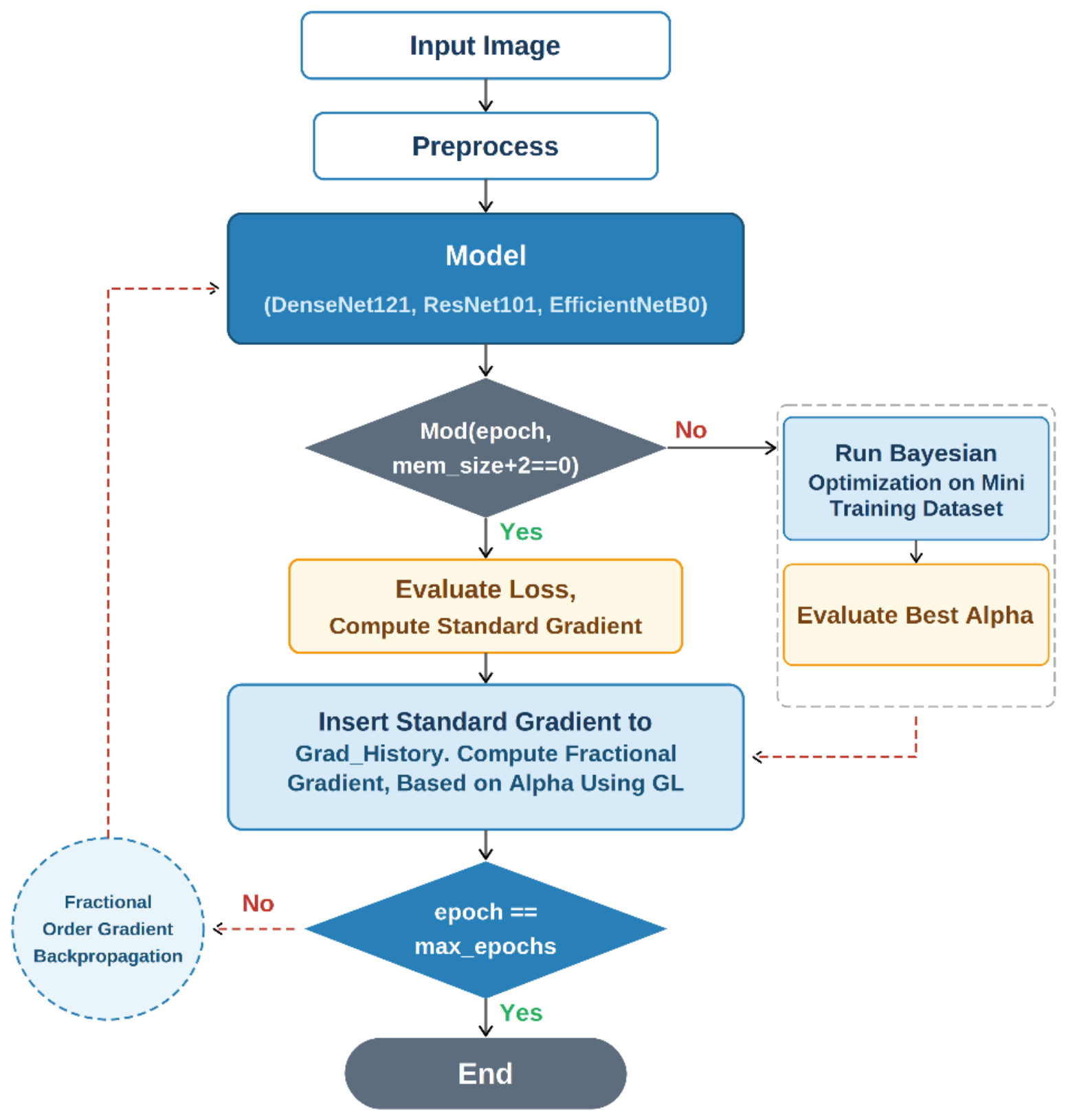
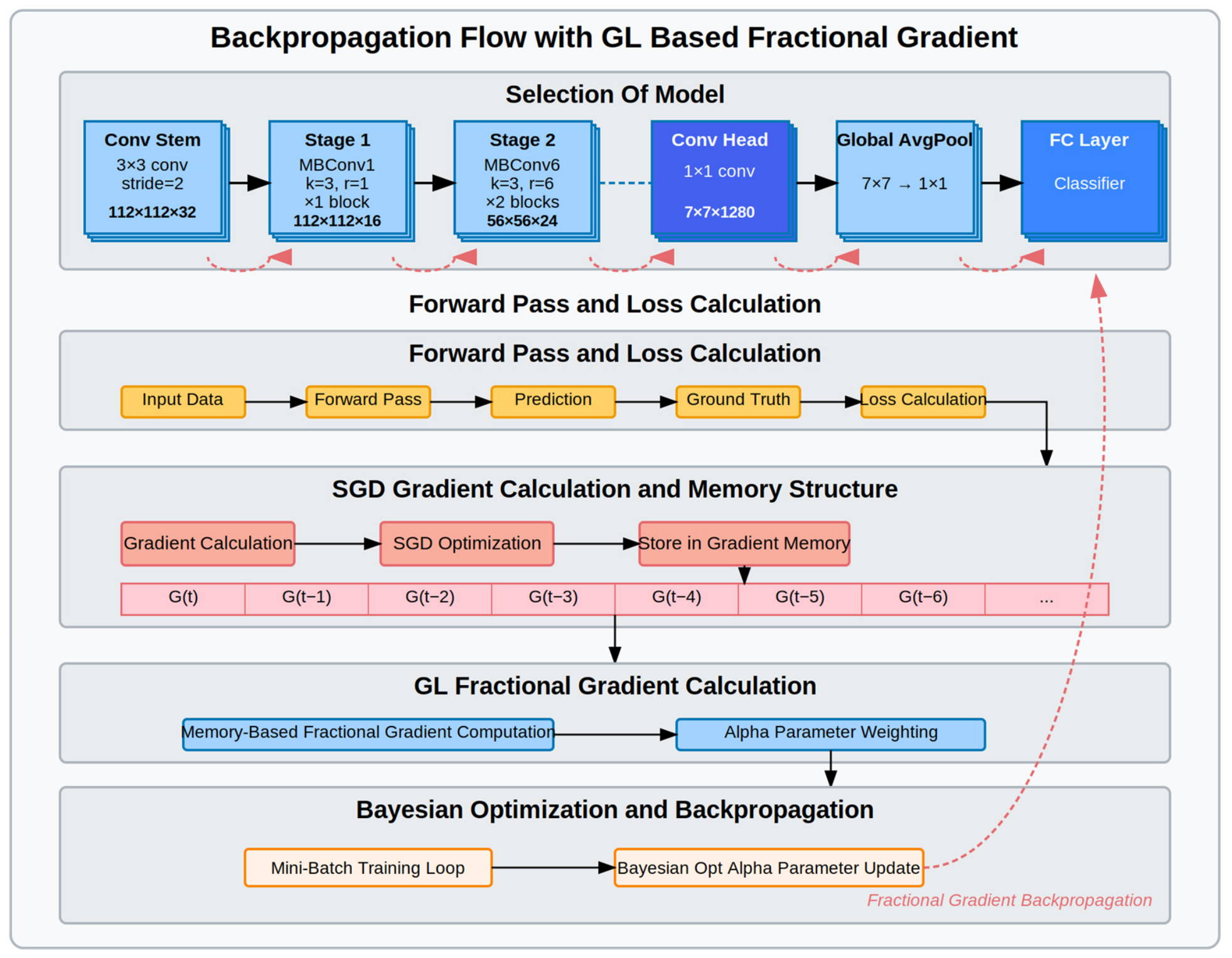
• A Bayesian optimization loop is embedded within the training process to dynamically select the optimal fractional order α at regular training intervals, eliminating the need for manual order selection and enabling architecture-specific adaptations.
• Fractional gradient backpropagation was implemented across all trainable layer types, namely the fully connected, batch normalization, and convolutional layers, providing comprehensive coverage of the network parameter space.
• Grad-CAM visualizations were employed to provide qualitative evidence that the performance gains reflect genuine improvements in discriminative feature learning rather than dataset-specific fitting.
• Comprehensive experiments on the IP102 benchmark demonstrate consistent accuracy improvements over standard gradient descent across three backbone architectures and two initialization strategies.

The remainder of this paper is organized as follows: Section 2 reviews related work on deep learning for pest classification, gradient-based optimization, and fractional calculus in machine learning; Section 3 describes the preliminary concepts, the IP102 dataset, the proposed fractional gradient method, and the experimental setup; Section 4 presents the experimental results; Section 5 provides discussion and analysis; and Section 6 concludes the paper.

2. Related Works

2.1. Deep Learning for Agricultural Pest Classification

Early automated pest classification approaches relied on handcrafted feature extraction techniques combined with traditional machine learning classifiers. Zhu et al. [15] proposed an automatic insect classification method that uses color histograms and the Gray-Level Co-occurrence Matrix to capture both color distribution and textural features. Huddar et al. [16] introduced an image-processing algorithm for detecting pests on plant leaves using a pipeline comprising color-space transformation, segmentation, noise reduction, and Moore neighborhood tracking. Zhao et al. [17] developed a classification method to identify sugarcane and cotton aphid pests by combining rough set theory with the fuzzy C-means clustering algorithm. While these approaches have demonstrated the feasibility of automated pest identification, their reliance on manually engineered features limits their ability to generalize across the broad morphological diversity observed in field conditions.

The introduction of deep convolutional neural networks has substantially advanced the state of the art in pest classification. Liu et al. [18] proposed a method for detecting and classifying paddy field pests by combining visual saliency maps with a deep CNN, enabling the model to focus on biologically relevant image regions. Xia et al. [19] introduced an improved VGG-based model that embedded a Region Proposal Network within the first convolutional layers, achieving precise pest localization while reducing the computational cost. Xie et al. [20] enhanced classification accuracy using a multi-level learning approach that combined handcrafted image features with deep learning representations, followed by dictionary learning to refine the extracted visual features. Visalli et al. [21] demonstrated the effectiveness of MobileNet, trained via transfer learning, for species-level insect recognition. In contrast, Liu et al. [22] proposed PestNet, an end-to-end deep learning framework incorporating position-sensitive score maps for large-scale multi-class pest detection and bounding-box regression. Aladhadh et al. [6] introduced a modified YOLOv5 architecture incorporating an extended Cross-Stage Partial module and an improved Selective Key attention module for real-time agricultural pest detection. Eze et al. [23] demonstrated that deep learning models that integrate image preprocessing techniques with support vector machine classification significantly outperform manual identification methods in both speed and accuracy.

More recent studies have specifically targeted the IP102 benchmark dataset, which presents substantial challenges due to its long-tailed class distribution across 102 pest species and over 75,000 images. Yang et al. [24] proposed a Convolutional Rebalancing Network to address the class imbalance inherent in large-scale rice pest datasets, achieving 70.42% classification accuracy on the IP102 dataset. Ayan et al. [25] employed a genetic algorithm-based weighted ensemble of deep convolutional neural networks for crop pest classification, reporting 67.13% accuracy on the same benchmark. Nanni et al. [26] presented a high-performing ensemble of multiple CNN models with a voting-based fusion strategy, achieving 74.11% accuracy, while Nguyen et al. [27] combined parallel multi-scale feature extraction with extensive data augmentation and ensemble predictions to achieve the current state-of-the-art accuracy of 76.44% on IP102. Collectively, these studies demonstrate that performance improvements in IP102 have been driven primarily by architectural complexity, ensemble strategies, and data augmentation, with the underlying optimization mechanism remaining largely unchanged across all approaches.

2.2. Gradient-Based Optimization in Deep Learning

Gradient descent and its variants constitute a foundational optimization framework for training deep neural networks. Ruder et al. [10] provided a comprehensive overview of the principal gradient descent algorithms, including stochastic gradient descent, mini-batch gradient descent, momentum-based methods, and adaptive learning-rate approaches such as AdaGrad, RMSprop, and Adam. Each of these methods introduces specific mechanisms to accelerate convergence or stabilize training; however, they share a common characteristic: parameter updates are computed exclusively from the current gradient, without any explicit mechanism to retain or exploit past gradient information. Bottou et al. [11] analyzed optimization methods for large-scale machine learning in detail and identified the key limitations of first-order gradient methods, including sensitivity to saddle points, dependence on learning-rate scheduling, and degraded convergence behavior under non-stationary loss landscapes.

These limitations are particularly consequential in the context of fine-grained pest classification on datasets with highly imbalanced class distributions, where the gradient signal for underrepresented classes is inherently sparse and unstable across successive training iterations. Despite the availability of numerous adaptive optimization algorithms, none of these approaches provides a principled mechanism for weighting gradient contributions by their temporal distance from the current update step. This absence of gradient memory is a structural limitation shared by all standard first-order optimization methods. It directly motivates the exploration of alternative formulations that incorporate historical gradient information in a mathematically grounded way.

2.3. Fractional Calculus in Machine Learning

Fractional calculus extends classical differential and integral operators to non-integer orders, enabling the modeling of memory-dependent and hereditary processes that cannot be adequately captured using integer-order derivatives. Duarte et al. [12] mathematically demonstrated the equivalence between different fractional derivative definitions and established the theoretical foundation linking fractional-order operators to memory-effective integration, showing that the fractional derivative in the range of −1 to 0 does not behave as a standard derivative but exhibits integral-like memory properties. Malkawi et al. [13], working in the context of potential theory, demonstrated that fractional integrals and derivatives can be formulated consistently for −1 < α ≤ 0 and α ≥ 0, showing that the results maintain the same form throughout.

The application of fractional calculus to gradient-based optimization in machine learning has attracted increasing interest. Aggarwal et al. [14] analyzed the convergence properties of an AT-CFGD variant of fractional gradient descent across smooth, strongly convex, and Hölder-smooth non-convex settings, proving linear and O(1/T) rates respectively under L-smoothness and bounded-gradient assumptions; the theoretical rates match those of standard gradient descent, while empirical experiments suggest practical speed-ups under well-chosen hyperparameters. However, existing fractional gradient descent formulations have two notable limitations. First, they typically employ a fixed positive fractional order, which prevents the model from dynamically adapting its gradient memory behavior in response to the evolving loss landscape during training. Second, they are generally evaluated in simplified optimization settings rather than in full CNN backpropagation pipelines applied to large-scale classification benchmarks. To the best of our knowledge, no prior study has jointly applied an extended Grünwald–Letnikov order range spanning both negative and positive fractional orders with adaptive Bayesian order tuning within a deep CNN-based optimization framework for agricultural pest classification. Collectively, the reviewed literature reveals a consistent pattern: performance improvements in agricultural pest classification have been pursued almost exclusively through architectural innovation, ensemble strategies, and data augmentation, while the underlying optimization mechanism has remained largely unexamined. Concurrently, fractional calculus offers a theoretically grounded framework for introducing gradient memory into neural network training. Yet, its application within full CNN backpropagation pipelines for large-scale classification benchmarks remains unexplored. The present study directly addresses this combined gap.

From a theoretical standpoint, the convergence behavior of fractional gradient descent for any fixed α has been established by Aggarwal et al. under standard smoothness and bounded gradient assumptions. The extension to the continuous range −1 < α < 1 with a ${\theta }_{\mathrm{scale}}$ = 1/Γ(α + 1) normalization factor preserves these guarantees, since it ${\theta }_{\mathrm{scale}}$ is a bounded positive constant for every α in this range. When α is updated at discrete intervals via Bayesian optimization, the resulting algorithm behaves as a piecewise fixed-α scheme; convergence within each piece follows directly from the fixed-α analysis, and stability across pieces is supported by the warm-up restriction of α to [−0.2, 0.2] during early epochs and by the requirement that the gradient buffer be fully populated before each optimizer invocation.

3. Materials and Methods

3.1. Preliminaries

3.1.1. DenseNet-121

DenseNet121, a prominent deep learning architecture, is characterized by a unique connectivity pattern that allows each layer to receive input from all preceding layers. This model comprises 121 layers, including 120 convolutional layers and a fully connected classification layer, thereby significantly enhancing feature propagation and mitigating the vanishing gradient problem commonly encountered in deep networks [28]. The architecture consists of dense blocks and transition layers. Within each dense block, each layer receives feature maps from all preceding layers as input and transmits its own feature maps to all subsequent layers. This structure maximizes feature reuse and enables better performance with fewer parameters. Transition layers are positioned between dense blocks and increase computational efficiency by reducing feature map dimensions [29].

DenseNet121 has proven to be highly effective in medical imaging, agricultural applications, and general object classification tasks. The architecture’s efficiency is enhanced by transition layers that reduce feature map dimensions and prevent overfitting, making it particularly suitable for real-time agricultural monitoring systems. Notably, it performs exceptionally well in scenarios with limited data availability, maintaining a high classification accuracy while requiring fewer parameters [30]. Figure 1 shows the architecture of DenseNet121 with multiple blocks connected in a dense connectivity pattern.

3.1.2. EfficientNet-B0

EfficientNetB0 is a deep learning architecture developed using a compound scaling method that jointly optimizes network depth, width, and resolution. This model is a lightweight architecture that operates effectively even on mobile devices and comprises MBConv (Mobile Inverted Bottleneck Convolution) blocks [31]. The architectural structure of EfficientNetB0 is based on MBConv blocks that incorporate squeeze-and-excitation modules and depthwise separable convolutions. Each block optimizes computational efficiency by first reducing, then increasing, the number of channels while maintaining feature representation capacity. This structure enables high performance using significantly fewer parameters than traditional CNN architectures. The model also improves gradient flow by utilizing the Swish activation function [32].

EfficientNetB0 delivers superior performance across diverse applications despite its compact structure, with demonstrated effectiveness spanning medical diagnosis and agricultural product analysis. Its optimized network design and low computational cost make it particularly suitable for mobile and embedded systems with limited hardware resources [31]. Figure 2 shows the architecture of EfficientNetB0, which illustrates its network layers and block structure.

3.1.3. ResNet-101

ResNet101 is a groundbreaking deep learning architecture that introduced a residual learning framework to address the challenges of training very deep neural networks. The model incorporates 101 layers structured around the innovative concept of residual connections, which facilitate gradient flow and enable effective training of deep networks [33]. The architectural foundation of ResNet101 consists of residual blocks, each employing skip connections to preserve and reuse input information throughout the network. These identity mappings allow the network to maintain and leverage features from earlier layers, effectively addressing the degradation problem that typically occurs in deep architecture networks. This design enables the model to learn both fine-grained and abstract features efficiently [34].

A distinguishing characteristic of ResNet101 is its ability to leverage extreme depth while maintaining stable training dynamics through its residual learning mechanism. The architecture has demonstrated remarkable versatility across complex visual recognition tasks, ranging from fine-grained classification to object detection. The robustness and generalization capabilities of ResNet101 make it particularly effective for applications that require high-level feature representation and intricate pattern recognition. Figure 3 shows the architecture of ResNet101, highlighting its deep network structure with multiple residual blocks.

3.1.4. Bayesian Optimization

Bayesian optimization is an efficient optimization technique in which the objective function is modeled using a Gaussian process, and the next evaluation point is selected using an acquisition function. This approach is particularly ideal for functions with expensive evaluations and is widely used in machine learning applications such as hyperparameter optimization [35].

Bayesian optimization constructs a probabilistic model of the objective function and selects the next most promising point based on this model. This process aims to achieve the global optimum with the fewest trials by establishing an optimal balance between exploration and exploitation [36]. This characteristic makes it an effective tool, particularly for the hyperparameter optimization of deep learning models [37].

3.2. IP102 Dataset

The IP102 dataset is a large-scale benchmark developed for automatic insect pest detection and classification, containing over 75,000 images of 102 insect pest species [38]. The dataset is publicly available at https://github.com/xpwu95/IP102 (accessed on 1 January 2026). Figure 4 shows the sample images from the IP102 dataset. IP102 presents significant challenges because of its broad species diversity and highly imbalanced class distribution. The dataset follows a long-tailed distribution, meaning that some pest classes contain significantly more images than others, making it difficult to learn rare pest species and leading to varying accuracy levels across different classes. Additionally, some images are low-resolution, blurry, or captured in noisy environments, making it particularly challenging for deep learning models to generalize. Moreover, approximately 19,000 images include bounding box annotations, making the dataset suitable for both image classification and object detection tasks.

In this study, the IP102 dataset was partitioned into 45,095 images for training, 7508 images for validation, and 22,619 images for testing. To focus on evaluating the proposed optimization approach in isolation, no preprocessing steps such as image enhancement or noise reduction were applied. The only modification was resizing all images to 224 × 224 × 3 to ensure compatibility with the deep learning architectures used.

3.3. Proposed Method

Deep learning models primarily rely on standard gradient descent for optimization, which iteratively updates the model parameters to minimize a given loss function. Although this method is widely used for its simplicity and effectiveness, recent studies have explored the potential benefits of fractional calculus for improving optimization performance. The growing interest in fractional-order derivatives has led to their application in various fields, including machine learning, physics, and engineering. Figure 5 illustrates the framework of the proposed method.

Fractional-order derivatives generalize the standard derivative by allowing the order to take any real value rather than only positive integers. For non-integer orders, the operator no longer depends only on the local neighborhood of the input but instead incorporates weighted contributions from past function values, the property commonly referred to as memory. The Grünwald–Letnikov formulation is the discretization most natural for gradient-descent settings because it expresses the fractional derivative as a finite weighted sum over historical samples, which directly matches the iteration-based structure of stochastic optimization. The negative-order regime exposes integral-like memory behavior while the positive-order regime corresponds to derivative-like behavior, motivating the extended range −1 < α < 1 used in this study.

In this study, the Grünwald–Letnikov (GL) fractional derivative approach was extended to cover the derivative range −1 < α < 1 and adapted for backpropagation in deep learning models. A modified fractional gradient is used instead of the standard gradient. During model operation, the best α value was determined via mini-training every 12 epochs, and the current α value was updated using a Bayesian optimizer to investigate its effects on model training efficiency and classification performance. Equation (1) shows the Grünwald–Letnikov fractional derivative, and Equation (2) shows the fractional binomial coefficients.

$$D^{\alpha }f(t)=\underset{\Delta \to 0}{\lim }{\displaystyle \frac{1}{{\Delta }^{\alpha }}}{\displaystyle \sum _{k=0}^{\infty }{(-1)}^k}\left(\begin{array}{c}\alpha \\ k\end{array}\right)f(t-k\Delta )$$

(1)

where $D^{\alpha }f(t)$ represents the fractional derivative of order α applied to function f(t), $\Delta$ is the step size, $k$ is the summation index, ${(-1)}^k\left(\begin{array}{c}\alpha \\ k\end{array}\right)$ represents the fractional binomial coefficient, defined in Equation (2);

$${(-1)}^k\left(\begin{array}{c}\alpha \\ k\end{array}\right)={(-1)}^k{\displaystyle \frac{\Gamma (\alpha +1)}{\Gamma (k+1)\Gamma (\alpha -k+1)}}$$

(2)

where is the Gamma function, which generalizes the factorial function. When we want to calculate the fractional gradient using the standard Grünwald–Letnikov method, we reconstruct the formula as shown in Equations (3) and (4).

$$g_{\mathrm{frac}}={\displaystyle \frac{1}{{\Delta }^{\alpha }}}{\displaystyle \sum _{k=0}^M{(-1)}^k}\left(\begin{array}{c}\alpha \\ k\end{array}\right)g_{k,\mathrm{history}}$$

(3)

where $g_{\mathrm{frac}}$ represents the fractional gradient computed using the Grünwald–Letnikov method, $k$ is the index of the memory size $M$, representing the position of past gradients used in the fractional gradient calculation. $\Delta$ is the step size (taken as 1), α is the fractional order of differentiation, is the memory length (determines how many past gradients are considered), is the gradient history values, and is the binomial coefficient for fractional order α as defined in Equation (2). Substituting this definition explicitly into Equation (3) yields the expanded formulation given in Equation (4);

$$g_{\mathrm{frac}}={\displaystyle \frac{1}{{\Delta }^{\alpha }}}{\displaystyle \sum _{k=0}^M{(-1)}^k}{\displaystyle \frac{\Gamma (\alpha +1)}{\Gamma (k+1)\Gamma (\alpha -k+1)}}{g}_{k,\mathrm{history}}$$

(4)

where is defined as above.

The general abstract gradient notation $g_{k,\mathrm{history}}$ introduced in Equation (3) is made explicit with respect to the corresponding layer $l$, neuron $i$, filter weights, and biases through the layer-specific gradient history terms formally defined in Equation (5);

$$g_{ij,k}^{[l]}:={\left.{\displaystyle \frac{\partial L}{\partial W_{ij}^{[l]}}}\right|}_{t-k}, g_{b,i,k}^{[l]}:={\left.{\displaystyle \frac{\partial L}{\partial b_i^{[l]}}}\right|}_{t-k}, g_{\gamma ,k}^{[l]}:={\left.{\displaystyle \frac{\partial L}{\partial {\gamma }^{[l]}}}\right|}_{t-k}, g_{\beta ,k}^{[l]}:={\left.{\displaystyle \frac{\partial L}{\partial {\beta }^{[l]}}}\right|}_{t-k}, g_{c,h,w,k}^{[l]}:={\left.{\displaystyle \frac{\partial L}{\partial W_{c,h,w}^{[l]}}}\right|}_{t-k}, g_{c,k}^{[l]}:={\left.{\displaystyle \frac{\partial L}{\partial b_c^{[l]}}}\right|}_{t-k}$$

(5)

where denotes the current training iteration, $k\in \{0,\dots ,M\}$ indexes the gradient history depth, $i$ denotes the neuron index for FC and BN layers, denotes the channel, height, and width indices for CNN filter weights, and denotes the channel index for CNN biases. Additionally, we $g_{b,i,k}^{[l]}$ denote the complete weight and bias gradient history of the FC layer at the training step $t-k$, stored as full parameter gradients. $g_{\gamma ,k}^{[l]}$ and $g_{\beta ,k}^{[l]}$ denote the gradient histories of the scale and shift parameters of the Batch Normalization layer at the training step $t-k$, respectively. This notation decouples the temporal offset from the layer index $l$. Per-sample, BN, and CNN variants are defined analogously: $g_{ij,k,s}^{[l]}$, $g_{b,i,k,s}^{[l]}$, $g_{\gamma ,k}^{[l]}$, $g_{\beta ,k}^{[l]}$, $g_{c,h,w,k}^{[l]}$, $g_{c,k}^{[l]}$ and collectively replace all ${|}_{t-k}$ superscript forms in the remainder of this section.

By applying the ${\theta }_{\mathrm{scale}}$ normalization to Equation (3), the gradient weights were adjusted to ensure more stable step progression as the model leveraged the memory effect of past gradients from the Bayesian optimization output. Simultaneously, this attenuation diminished when the model tended to follow the trajectory of the new gradients. Equation (6) shows the applied equation, and Equation (7) shows the ${\theta }_{\mathrm{scale}}$ applied equation:

$${\theta }_{\mathrm{scale}}={\displaystyle \frac{1}{\Gamma (\alpha +1)}}$$

(6)

$$g_{\mathrm{frac}}={\displaystyle \frac{1}{{\Delta }^{\alpha }\Gamma (\alpha +1)}}{\displaystyle \sum _{k=0}^M{(-1)}^k}\left(\begin{array}{c}\alpha \\ k\end{array}\right)g_{k,\mathrm{history}}$$

(7)

Then, the formulation is regenerated using the logarithmic form of the Gamma function rather than the standard Gamma function to ensure numerical stability, avoid overflow errors, and improve computational efficiency in the Grünwald–Letnikov formulation. This transformation converts division into subtraction, thereby reducing precision loss and making calculations more stable. Equation (8) shows the logarithmic form of Equation (7);

$$g_{\mathrm{frac}}={\displaystyle \frac{1}{\Gamma (\alpha +1){\Delta }^{\alpha }}}{\displaystyle \sum _{k=0}^M{(-1)}^k}\exp (\log \Gamma (\alpha +1)-[\log \Gamma (k+1)+\log \Gamma (\alpha -k+1)])g_{k,\mathrm{history}}$$

(8)

For implementation purposes, Equation (8) constitutes the numerically stable form employed throughout the codebase, where all Gamma function evaluations are performed via their logarithmic equivalents (‘lgamma’) to prevent overflow and improve precision. Throughout the remainder of this section, the algebraic binomial coefficient notation in Equation (7) is retained for theoretical clarity; in practice, all gamma function evaluations are performed via their logarithmic equivalents, as described above. In practice, each binomial coefficient $\left(\begin{array}{c}\alpha \\ k\end{array}\right)$ is evaluated using the identity:

$$\left(\begin{array}{c}\alpha \\ k\end{array}\right)=\exp [\log \Gamma (\alpha +1)-\log \Gamma (k+1)-\log \Gamma (\alpha -k+1)]$$

and the factor is computed as ${\displaystyle \frac{1}{\exp (\log \Gamma (\alpha +1))}}$, as shown in Equation (8).

Equations (9) and (10) represent the standard gradient backpropagation for weight and bias, respectively. Equations (11) and (12) describes the fractional gradient backpropagation formulated based on the Grünwald–Letnikov (GL) fractional derivative.

Substituting the explicit gradient history definitions from Equation (5) into Equations (11) and (12) yields the time-indexed formulations in Equations (13) and (14).

$${\displaystyle \frac{\partial L}{\partial W_{ij}^{[l]}}}={\displaystyle \frac{\partial L}{\partial a_i^{[l]}}}{f}^{(1)}(z_i^{[l]})A_j^{[l-1]}$$

(9)

$${\displaystyle \frac{\partial L}{\partial b_i^{[l]}}}={\displaystyle \frac{\partial L}{\partial a_i^{[l]}}}{f}^{(1)}(z_i^{[l]})$$

(10)

$${\displaystyle \frac{{\partial }^{\alpha }L}{\partial W_{ij}^{[l]}}}={\displaystyle \frac{1}{{\Delta }^{\alpha }\Gamma (\alpha +1)}}{\displaystyle \sum _{k=0}^M{(-1)}^k}\left(\begin{array}{c}\alpha \\ k\end{array}\right)g_{ij,k}^{[l]}$$

(11)

$${\displaystyle \frac{{\partial }^{\alpha }L}{\partial b_i^{[l]}}}={\displaystyle \frac{1}{{\Delta }^{\alpha }\Gamma (\alpha +1)}}{\displaystyle \sum _{k=0}^M{(-1)}^k}\left(\begin{array}{c}\alpha \\ k\end{array}\right)g_{b,i,k}^{[l]}$$

(12)

$${\displaystyle \frac{{\partial }^{\alpha }L}{\partial W_{ij}^{[l]}}}={\displaystyle \frac{1}{{\Delta }^{\alpha }\Gamma (\alpha +1)}}{\displaystyle \sum _{k=0}^M{(-1)}^k}\left(\begin{array}{c}\alpha \\ k\end{array}\right){\displaystyle \frac{\partial L}{\partial a_i^{[l]}}}{|}_{t-k}·f^{(1)}\left(z_i^{[l]}\right){|}_{t-k}·A_j^{[l-1]}{|}_{t-k}$$

(13)

$${\displaystyle \frac{{\partial }^{\alpha }L}{\partial b_i^{[l]}}}={\displaystyle \frac{1}{{\Delta }^{\alpha }\Gamma (\alpha +1)}}{\displaystyle \sum _{k=0}^M{(-1)}^k}\left(\begin{array}{c}\alpha \\ k\end{array}\right){\displaystyle \frac{\partial L}{\partial a_i^{[l]}}}{|}_{t-k}·f^{(1)}\left(z_i^{[l]}\right){|}_{t-k}$$

(14)

where $z_i^{[l]}$ denotes the pre-activation output (linear transformation result) of neuron $i$ at layer $l$, $a_i^{[l]}=f(z_i^{[l]})$ denotes the corresponding post-activation output, $A_j^{[l-1]}$ denotes the activated output of neuron $j$ at the preceding layer $l-1$, $f^{(1)}(z_i^{[l]})$ denotes the derivative of the activation function evaluated at $z_i^{[l]}$, and ${\displaystyle \frac{\partial L}{\partial a_i^{[l]}}}{|}_{t-k}$ denotes the loss gradient with respect to the activated output of neuron $i$ at layer $l$, evaluated at training step $t-k$. The batch-averaged versions of Equation (13) and Equation (14) are given by Equation (15) and Equation (16), respectively.

$${\displaystyle \frac{{\partial }^{\alpha }L}{\partial W_{ij}^{[l]}}}={\displaystyle \frac{1}{m{\Delta }^{\alpha }\Gamma (\alpha +1)}}{\displaystyle \sum _{s=1}^m{\displaystyle \sum _{k=0}^M{(-1)}^k}}\left(\begin{array}{c}\alpha \\ k\end{array}\right)g_{ij,k,s}^{[l]}$$

(15)

$${\displaystyle \frac{{\partial }^{\alpha }L}{\partial b_i^{[l]}}}={\displaystyle \frac{1}{m{\Delta }^{\alpha }\Gamma (\alpha +1)}}{\displaystyle \sum _{s=1}^m{\displaystyle \sum _{k=0}^M{(-1)}^k}}\left(\begin{array}{c}\alpha \\ k\end{array}\right)g_{b,i,k,s}^{[l]}$$

(16)

where m represents the batch size (total number of samples in a batch). $s$ is the index that iterates over each sample in the batch. $a_{js}^{[l-1]}$ represents the activation value of the j th neuron in the s th sample at layer, $(l-1)$. $f^{(1)}(z_{is}^{[l]})$, denotes the derivative of the activation function for the i th neuron in the s th sample. $g_{i,j,k,s}^{[l]}$, $g_{b,i,k,s}^{[l]}$ are the gradient history term as defined in Equation (5), representing the standard gradient of weight $W_{ij}^{[l]}$ and bias $b_i^{[l]}$ at layer $l$, stored at training step $t-k$ for sample $s$.

In this study, gradients update the trainable parameters of the model. Consequently, parameter updates are applied in the Fully Connected (FC) layer, Batch Normalization (BN) layer, and Convolutional Neural Network (CNN) layers. Equations (17) and (18) represent the parameter updates performed using the classical backpropagation algorithm in the FC layer. Equations (19) and (20) illustrate the parameter updates performed using the Grünwald–Letnikov (GL) fractional derivative method. Finally, Equations (21) and (22) present the parameter updates performed using the Grünwald–Letnikov fractional derivative method, adjusted according to a batch size of m.

$$W_{ij}^{[l]}\leftarrow W_{ij}^{[l]}-\eta {\displaystyle \frac{\partial L}{\partial W_{ij}^{[l]}}}$$

(17)

$$b_i^{[l]}\leftarrow b_i^{[l]}-\eta {\displaystyle \frac{\partial L}{\partial b_i^{[l]}}}$$

(18)

$$W_{ij}^{[l]}\leftarrow W_{ij}^{[l]}-\eta {\displaystyle \frac{1}{{\Delta }^{\alpha }\Gamma (\alpha +1)}}{\displaystyle \sum _{k=0}^M{(-1)}^k}\left(\begin{array}{c}\alpha \\ k\end{array}\right)g_{ij,k}^{[l]}$$

(19)

$$b_i^{[l]}\leftarrow b_i^{[l]}-\eta {\displaystyle \frac{1}{{\Delta }^{\alpha }\Gamma (\alpha +1)}}{\displaystyle \sum _{k=0}^M{(-1)}^k}\left(\begin{array}{c}\alpha \\ k\end{array}\right)g_{b,i,k}^{[l]}$$

(20)

$$W_{ij}^{[l]}\leftarrow W_{ij}^{[l]}-\eta {\displaystyle \frac{1}{m{\Delta }^{\alpha }\Gamma (\alpha +1)}}{\displaystyle \sum _{s=1}^m{\displaystyle \sum _{k=0}^M{(-1)}^k}}\left(\begin{array}{c}\alpha \\ k\end{array}\right)g_{ij,k,s}^{[l]}$$

(21)

$$b_i^{[l]}\leftarrow b_i^{[l]}-\eta {\displaystyle \frac{1}{m{\Delta }^{\alpha }\Gamma (\alpha +1)}}{\displaystyle \sum _{s=1}^m{\displaystyle \sum _{k=0}^M{(-1)}^k}}\left(\begin{array}{c}\alpha \\ k\end{array}\right)g_{b,i,k,s}^{[l]}$$

(22)

Equations (23) and (24) represent the parameter updates performed using the classical backpropagation algorithm in the Batch Normalization (BN) layer. Equations (25) and (26) illustrate the parameter updates obtained using the Grünwald–Letnikov (GL) fractional derivative method. Finally, Equations (27) and (28) present the parameter updates obtained using the Grünwald–Letnikov fractional derivative method, adjusted for a batch size of m.

$${\gamma }^{[l]}\leftarrow {\gamma }^{[l]}-\eta {\displaystyle \frac{\partial L}{\partial {\gamma }^{[l]}}}$$

(23)

$${\beta }^{[l]}\leftarrow {\beta }^{[l]}-\eta {\displaystyle \frac{\partial L}{\partial {\beta }^{[l]}}}$$

(24)

$${\gamma }^{[l]}\leftarrow {\gamma }^{[l]}-\eta {\displaystyle \frac{1}{{\Delta }^{\alpha }\Gamma (\alpha +1)}}{\displaystyle \sum _{k=0}^M{(-1)}^k}\left(\begin{array}{c}\alpha \\ k\end{array}\right)g_{\gamma ,k}^{[l]}$$

(25)

$${\beta }^{[l]}\leftarrow {\beta }^{[l]}-\eta {\displaystyle \frac{1}{{\Delta }^{\alpha }\Gamma (\alpha +1)}}{\displaystyle \sum _{k=0}^M{(-1)}^k}\left(\begin{array}{c}\alpha \\ k\end{array}\right)g_{\beta ,k}^{[l]}$$

(26)

$${\gamma }^{[l]}\leftarrow {\gamma }^{[l]}-\eta {\displaystyle \frac{1}{m{\Delta }^{\alpha }\Gamma (\alpha +1)}}{\displaystyle \sum _{s=1}^m{\displaystyle \sum _{k=0}^M{(-1)}^k}}\left(\begin{array}{c}\alpha \\ k\end{array}\right)g_{\gamma ,k,s}^{[l]}$$

(27)

$${\beta }^{[l]}\leftarrow {\beta }^{[l]}-\eta {\displaystyle \frac{1}{m{\Delta }^{\alpha }\Gamma (\alpha +1)}}{\displaystyle \sum _{s=1}^m{\displaystyle \sum _{k=0}^M{(-1)}^k}}\left(\begin{array}{c}\alpha \\ k\end{array}\right)g_{\beta ,k,s}^{[l]}$$

(28)

Equations (29) and (30) represent the parameter updates performed using the classical backpropagation algorithm in the Convolutional Neural Network (CNN) layer. Equations (31) and (32) illustrate the parameter updates obtained using the Grünwald–Letnikov (GL) fractional derivative method. Finally, Equations (33) and (34) present the parameter updates performed using the Grünwald–Letnikov fractional derivative method, adjusted according to a batch size of m:

$$W_{c,h,w}^{[l]}\leftarrow W_{c,h,w}^{[l]}-\eta {\displaystyle \frac{\partial L}{\partial W_{c,h,w}^{[l]}}}$$

(29)

$$b_c^{[l]}\leftarrow b_c^{[l]}-\eta {\displaystyle \frac{\partial L}{\partial b_c^{[l]}}}$$

(30)

$$W_{c,h,w}^{[l]}\leftarrow W_{c,h,w}^{[l]}-\eta {\displaystyle \frac{1}{{\Delta }^{\alpha }\Gamma (\alpha +1)}}{\displaystyle \sum _{k=0}^M{(-1)}^k}\left(\begin{array}{c}\alpha \\ k\end{array}\right)g_{c,h,w,k}^{[l]}$$

(31)

$$b_c^{[l]}\leftarrow b_c^{[l]}-\eta {\displaystyle \frac{1}{{\Delta }^{\alpha }\Gamma (\alpha +1)}}{\displaystyle \sum _{k=0}^M{(-1)}^k}\left(\begin{array}{c}\alpha \\ k\end{array}\right)g_{c,k}^{[l]}$$

(32)

$$W_{c,h,w}^{[l]}\leftarrow W_{c,h,w}^{[l]}-\eta {\displaystyle \frac{1}{m{\Delta }^{\alpha }\Gamma (\alpha +1)}}{\displaystyle \sum _{s=1}^m{\displaystyle \sum _{k=0}^M{(-1)}^k}}\left(\begin{array}{c}\alpha \\ k\end{array}\right)g_{c,h,w,k,s}^{[l]}$$

(33)

$$b_c^{[l]}\leftarrow b_c^{[l]}-\eta {\displaystyle \frac{1}{m{\Delta }^{\alpha }\Gamma (\alpha +1)}}{\displaystyle \sum _{s=1}^m{\displaystyle \sum _{k=0}^M{(-1)}^k}}\left(\begin{array}{c}\alpha \\ k\end{array}\right)g_{c,k,s}^{[l]}$$

(34)

where represents the weights of the filter in the c-th channel with a size of h × w. $b_c^{[l]}$, represents the bias value of the c-th channel.

Unlike most existing fractional-order optimization methods, which typically employ a fixed positive fractional order and are limited to conventional optimization settings, our approach extends the Grünwald–Letnikov (GL) formulation to the continuous range of −1 < α < 1. This extension enables the model to capture both derivative-like and integral-like memory dynamics during training. Furthermore, instead of using a static fractional order, we embedded $\alpha$ within a Bayesian optimization loop, allowing dynamic and architecture-specific adaptation throughout training. The combination of an extended GL order range with adaptive order tuning constitutes a dual innovation that distinguishes AFGD from previous fractional gradient descent approaches. To the best of our knowledge, this joint formulation has not been previously applied to deep CNN-based optimization for agricultural pest classification.

3.4. Experimental Setup

3.4.1. Hardware and Dataset Configuration

The study was conducted on Google Colab (Google LLC, Mountain View, CA, USA) using an NVIDIA A100-SXM4-80GB GPU (NVIDIA Corporation, Santa Clara, CA, USA). All experiments were implemented in Python 3.12 (Python Software Foundation, Wilmington, DE, USA) with TensorFlow 2.20 and the Keras API (Google LLC, Mountain View, CA, USA). The fractional order α was optimized using the open-source bayesian-optimization library (v3.3.0), with scikit-learn 1.6.1, OpenCV 4.13.0, and NumPy 2.0.2 as supporting libraries. The proposed method was tested on the ResNet101, DenseNet121, and EfficientNetB0 backbones, both in their untrained and pretrained ImageNet forms. To focus on the effectiveness of the proposed method, preprocessing steps such as image enhancement were avoided. Only data normalization was applied to the input images to ensure consistency in the distribution of pixel values.

3.4.2. Training Hyperparameters

During training, all models were optimized using the SGD optimizer with a learning rate of 0.004 and a momentum of 0.9. Moreover, to better evaluate the method’s effectiveness, techniques such as dropout and adaptive learning rates were not applied, ensuring that the models were trained in their purest forms. Figure 6 illustrates the architecture and workflow of the proposed fractional gradient backpropagation approach.

All SGD-based runs share the learning rate of 0.004 and momentum of 0.9. The Adam and AdamW baselines reported in Section 4 use the learning rate of 0.001 recommended in their original papers, with AdamW additionally applying a weight-decay coefficient of 0.01. No adaptive learning rate scheduler is applied to any run.

3.4.3. Fractional Gradient Configuration

The fractional gradient computation was restricted within the range of α ∈ [−1, 1]. Instead of concentrating on higher-order gradient derivatives through partial differentiation, this study examines the feasibility of achieving optimal gradient flow by investigating the derivative spectrum ranging from negative first to positive first order.

Another objective of this study was to examine whether the method prefers to adapt to new gradients or to maintain a gradient memory, based on the stored gradient history. Rather than determining the optimal derivative order, we aimed to leverage a specific range of fractional derivatives to enable the model to better adapt to dynamic real-world conditions.

Because real-world environments exhibit dynamic, variable characteristics rather than static, stable ones, this study adopts an approach in which a fixed derivative order does not determine the gradient flow. Instead, the model dynamically adjusts its optimization strategy based on the data distribution and learning process.

This is analogous to the strategy of a navigator on a foggy road who must continuously reassess the environment rather than relying solely on prior observations, as committing too strongly to past information risks poor decisions when conditions change. Similarly, fixing the gradient flow to a predetermined derivative order prevents the model from adapting to the evolving loss landscape during training.

While controlling the fractional derivative flow between −1 and 1, if Bayesian optimization found the best alpha in the negative derivative, it would mean the method would want to use gradient memory for the next gradient. Similarly, when it tended towards the +1 derivative, this would indicate that it was in search of a new gradient. ${\theta }_{\mathrm{scale}}={\displaystyle \frac{1}{\Gamma (\alpha +1)}}$ normalization was used to enable it to take smaller, more stable steps when using memory and to exhibit more aggressive behavior in search of new gradients.

To observe the effects of the used −1 < α < 1 derivative order ${\theta }_{\mathrm{scale}}$, a Bayesian Optimizer was called at regular intervals to find the optimal α fractional derivative order, which was then returned to the main model.

3.4.4. Bayesian Optimization Protocol

To mitigate critical issues such as abrupt alpha transitions (the “alpha jump” problem) and stagnation in model convergence at suboptimal performance levels (“convergence stagnation”), a manual warm-up strategy was employed during the initial training epochs. In this phase, the α range was deliberately restricted to [−0.2, 0.2] to enable a smoother transition into the fractional optimization regime and allow the gradient memory to be populated gradually and steadily. This strategy was intended to prevent the destabilizing effects of sudden transitions between positive and negative fractional characteristics and to help the model better adapt to its optimization landscape.

In the Bayesian Optimizer, a mini-training process was run on 1% of the training and validation data to determine the best value for the main model to continue with. Furthermore, in this study, the standard gradient was stored in a memory buffer called grad_history at each step, and its elements were used in the GL fractional gradient calculation along with the incoming gradient for the next step. To avoid slowing down the model and to observe the memory effect, the grad_history value was set to 10 for all the models. Because it was desired that each α value should be called after at least as many epochs as the minimum memory amount for full effect during operation, the Bayesian optimizer was run every 12 epochs. At each invocation, the Bayesian optimizer performed 25 evaluations (10 random exploration points followed by 15 guided iterations) over a stratified subset comprising 1% of the training and validation data (197 batches), ensuring a representative class coverage. Over the 50-epoch training process, the optimizer was invoked four times.

The fractional derivative range, theoretically accepted as (−1, 1), caused the fractional gradient to vanish after −0.9 due to the ${\theta }_{\mathrm{scale}}$ normalization used. Therefore, during the coding phase, the alpha range was set to (−0.9, 0.99) to prevent potential gradient-vanishing problems. All deep learning models used in the study were trained for 100 epochs with standard gradient-based optimization on the datasets, whereas all models were trained for 50 epochs with our proposed method.

The same gradient-memory length M is used uniformly across the fully connected, batch-normalization, and convolutional layers, since all trainable parameters are updated at the same iteration cadence and therefore share a common temporal structure for the gradient history. The choice M = 10 is justified on three grounds: First, the empirical sweep shows that test accuracy is essentially flat across M ∈ {5, 10, 20}. Second, for the gradient buffer to be fully populated under any given α before the next Bayesian invocation, M must remain below the 12-epoch invocation interval. Third, increasing M from 10 to 20 doubles both the gradient-buffer memory and the per-step fractional FLOPs for an accuracy gain below 0.1 percentage points, an unfavorable trade-off. M = 10, therefore, sits at the intersection of the accuracy plateau, the invocation-interval coupling, and the computational cost.

3.5. Convergence: Theoretical Positioning

Existing convergence analyses for fractional gradient descent, including the linear and O(1/T) rates established by Aggarwal [14] for an AT-CFGD variant of the Caputo derivative, formulate the gradient update as a fractional derivative evaluated at a single point. The Grünwald–Letnikov formulation employed in this study, constructed as a truncated weighted sum over a finite gradient-history buffer, lies outside the direct scope of these results. A complete convergence theorem for this class of methods remains an open problem.

The Bayesian optimizer updates α at fixed intervals of T_B epochs, producing a piecewise-constant α(t) profile under which the method reduces to fixed-α fractional gradient descent within each interval. Two design conditions preserve this fixed-α regime across the training trajectory. (i) Memory–interval relation M ≤ T_B ensures that the gradient buffer is fully refreshed between successive α values; otherwise, the buffer would mix gradients from multiple α regimes. (ii) Bounded α range keeps the normalization factor ${\theta }_{\mathrm{scale}}={\displaystyle \frac{1}{\Gamma (\alpha +1)}}$ bounded over the practical range α ∈ [−0.9, 0.99] adopted in Section 3.4.4, constraining the effective step size within a fixed multiplicative band and preventing divergence at piecewise transitions.

4. Results

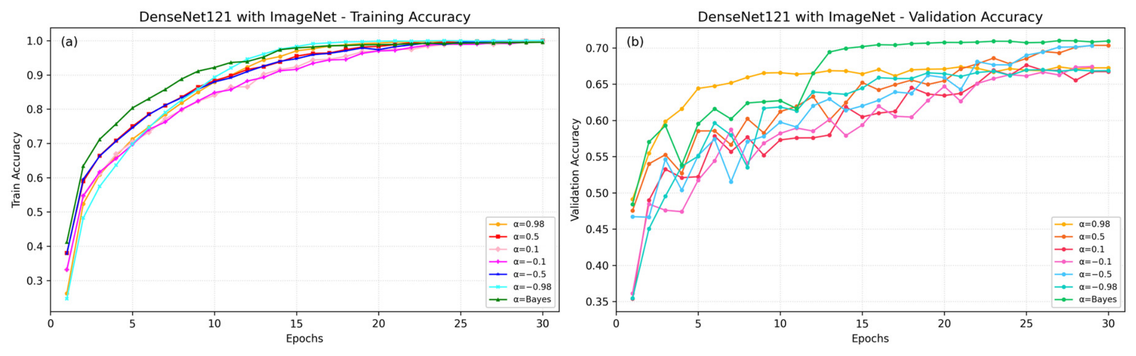
The proposed method was evaluated in both untrained and ImageNet-pretrained settings. Figure 7 illustrates the training and validation accuracies for different fractional orders (α = −0.98, −0.5, −0.1, 0.1, 0.5, 0.98) and the Bayesian-optimized α using DenseNet121 with ImageNet pretraining.

Table 1. Top-1 classification accuracy of untrained models on the IP102 dataset.

	DenseNet121	ResNet101	EfficientNetB0
Standard Gradient	35.75 (%)	33.03 (%)	35.32 (%)
Proposed Method	56.48 (%)	44.54 (%)	46.33 (%)

reports the top-1 classification accuracy of untrained ResNet101, DenseNet121, and EfficientNetB0 models on the IP102 dataset, using standard gradient descent and the proposed GL-based fractional gradient backpropagation.

Table 2. Top-1 classification accuracy of ImageNet pre-trained models on the IP102 dataset.

	DenseNet121	ResNet101	EfficientNetB0
Standard Gradient	64.12 (%)	62.50 (%)	66.40 (%)
Proposed Method	70.81 (%)	69.89 (%)	70.16 (%)

presents the top-1 classification accuracy of ImageNet pre-trained models evaluated under the same conditions.

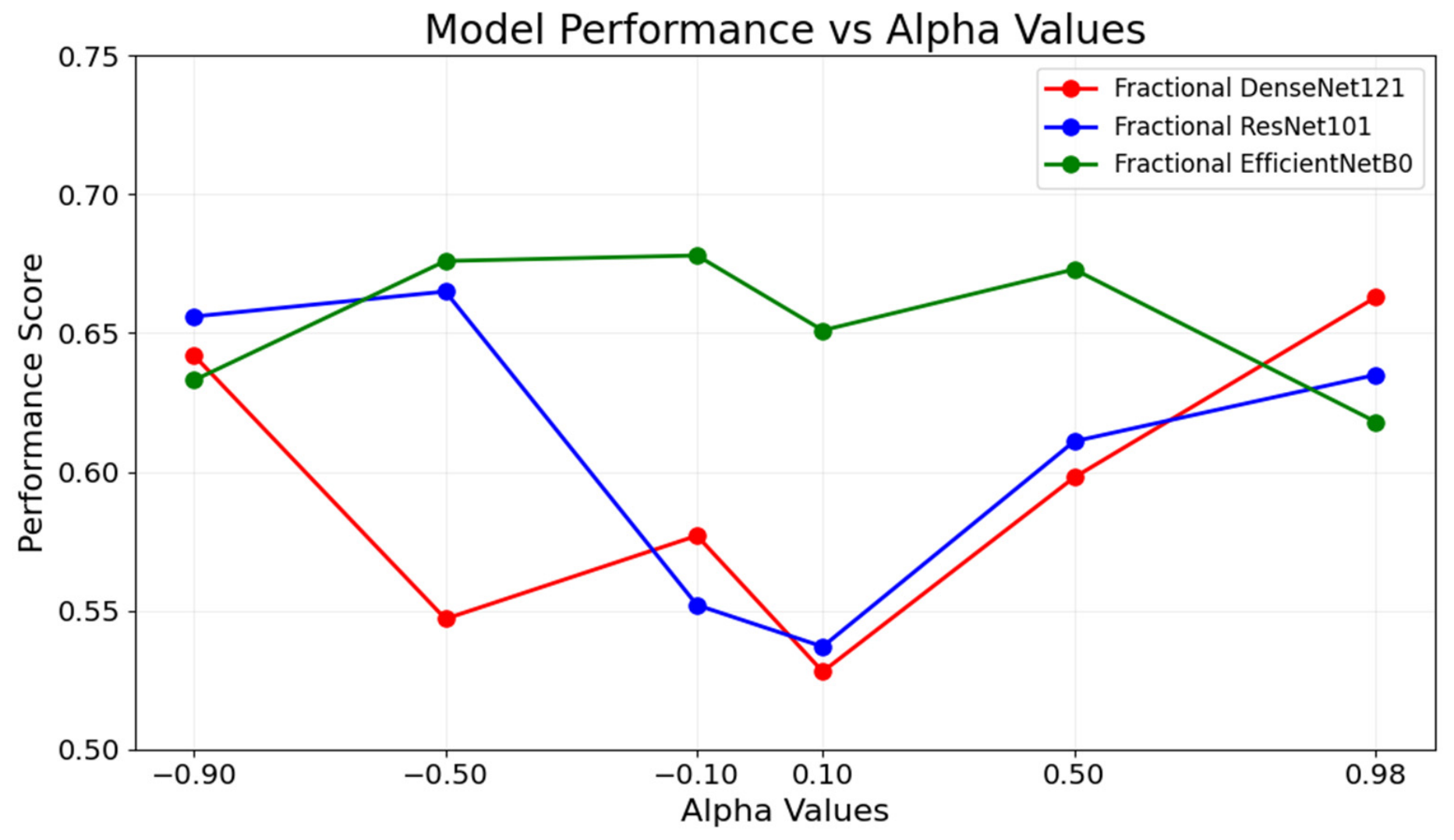
Figure 8 demonstrates the performance of all three ImageNet pre-trained models across varying fractional derivative orders without ${\theta }_{\mathrm{scale}}$ normalization or Bayesian optimization. Different alpha values consistently achieved improved classification performance compared to standard gradient descent, supporting the hypothesis that gradient flow control through fractional-order derivatives represents a more consistent optimization strategy.

On the IP102 dataset, untrained networks using fractional gradient backpropagation showed measurable improvements over their standard gradient counterparts. Absolute test accuracy increased from 35.75% to 56.48% for DenseNet121 (an absolute gain of 20.73 percentage points), from 33.03% to 44.54% for ResNet101 (11.51-pp absolute gain), and from 35.32% to 46.33% for EfficientNetB0 (11.01-pp absolute gain). We note that while these absolute gains are substantial, the absolute accuracy levels in the untrained configuration remain modest and not deployment-ready; the untrained results are reported only to isolate the contribution of the fractional gradient mechanism in the absence of pre-trained feature transfer.

For the ImageNet pre-trained models, the fractional gradient DenseNet121 reached 70.81% test accuracy (an absolute improvement of 6.69 percentage points over the 64.12% standard gradient baseline, 10.43% relative), ResNet101 reached 69.89% (a 7.39-pp absolute gain, 11.82% relative), and EfficientNetB0 reached 70.16% (a 3.76-pp absolute gain, 5.66% relative). These absolute gains are moderate; we emphasize that they are achieved with no architectural modification, no additional data augmentation, and no learning-rate scheduling, isolating the contribution of the optimization mechanism alone. The final performance gains were obtained with the alpha values that yielded the lowest validation loss in the Bayesian optimizer: α = −0.87 for DenseNet121, α = −0.90 for ResNet101, and α = 0.98 for EfficientNetB0.

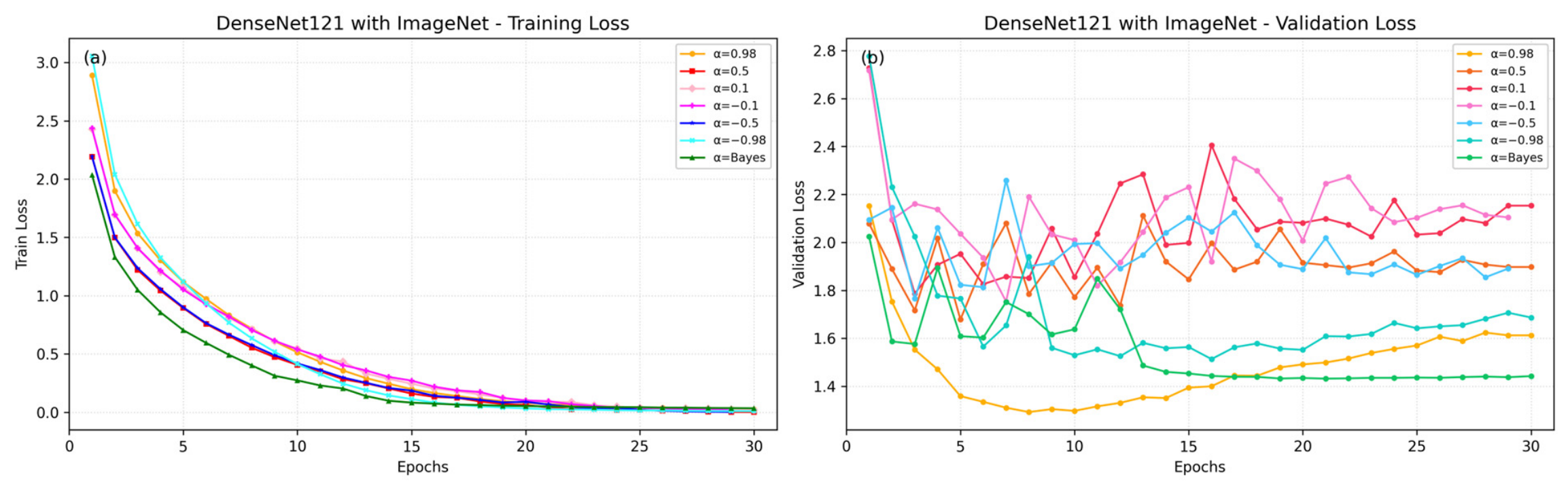
Figure 9 shows training and validation loss for different alpha values and for the Bayesian-optimized alpha, using DenseNet121 with ImageNet pre-training.

Table 3. Detailed performance comparison of standard and fractional gradient models (DenseNet121, EfficientNetB0, ResNet101) with ImageNet pre-training on the IP102 dataset.

Metric	Standard DenseNet121	Fractional DenseNet121	Standard EfficientNetB0	Fractional EfficientNetB0	Standard ResNet101	Fractional ResNet101
Accuracy	64.12 (%)	70.81 (%)	66.40 (%)	70.16 (%)	62.50 (%)	69.89 (%)
F1	52.82 (%)	63.76 (%)	59.92 (%)	61.20 (%)	52.78 (%)	62.43 (%)
Precision	58.08 (%)	65.22 (%)	63.57 (%)	63.38 (%)	59.73 (%)	63.64 (%)
Recall	53.01 (%)	62.93 (%)	58.59 (%)	60.44 (%)	51.21 (%)	61.66 (%)
Training Time	2 h 32 m 05 s	3 h 02 m 42 s	1 h 27 m 41 s	1 h 32 m 01 s	3 h 09 m 40 s	3 h 39 m 07 s

presents a detailed performance comparison of standard gradient models trained for 100 epochs and fractional gradient models trained for 50 epochs, covering DenseNet121, EfficientNetB0, and ResNet101 with ImageNet pre-training and reporting accuracy, F1, precision, recall, and training time on the IP102 dataset.

As shown in Table 3, the fractional-gradient variant consistently outperforms its standard-gradient counterpart across all three architectures. DenseNet121 achieves a 10.43% relative improvement in accuracy (70.81% vs. 64.12%), with superior F1 (0.6376 vs. 0.5282), precision (0.6522 vs. 0.5808), and recall (0.6293 vs. 0.5301). ResNet101 yields the highest relative gain of 11.82% (69.89% vs. 62.50%), accompanied by improvements in F1 (0.6243 vs. 0.5278), precision (0.6364 vs. 0.5973), and recall (0.6166 vs. 0.5121). EfficientNetB0 demonstrates a more modest improvement of 5.66% (70.16% vs. 66.40%), with gains in F1 (0.6120 vs. 0.5992) and recall (0.6044 vs. 0.5859) across all 102 pest classes. These performance gains are accompanied by increased training times, with fractional optimization requiring approximately 1.2, 1.05, and 1.16 times as much training time for DenseNet121, EfficientNetB0, and ResNet101, respectively, due to Bayesian optimization overhead and gradient history maintenance. To further assess the stability of the proposed method,

Table 4. Reproducibility analysis of the proposed fractional gradient method across three independent training runs on the IP102 dataset (ImageNet pre-trained). Standard deviations below ±0.5% and 95% confidence intervals computed via t-distribution (df = 2) confirm that the reported gains are stable across runs. Critically, the lower bound of each confidence interval exceeds the corresponding standard gradient baseline reported in Table 2, confirming that the observed improvements are statistically robust and not attributable to a single favorable run.

Configuration	Run 1 (%)	Run 2 (%)	Run 3 (%)	Mean ± Std (%)	%95 CI
Fractional DenseNet121	70.61	70.73	70.81	70.72 ± 0.10	[70.47, 70.97]
Fractional ResNet101	69.89	69.61	69.23	69.58 ± 0.33	[68.76, 70.40]
Fractional EfficientNetB0	69.94	70.16	70.04	70.05 ± 0.11	[69.78, 70.32]

reports the top-1 classification accuracy across three independent training runs for all fractional-gradient configurations. Standard deviations of ±0.10%, ±0.33%, and ±0.11% for DenseNet121, ResNet101, and EfficientNetB0 confirm that the observed gains are consistent across runs. The corresponding 95% confidence intervals, computed via t-distribution (df = 2), are [70.47, 70.97], [68.76, 70.40], and [69.78, 70.32] for DenseNet121, ResNet101, and EfficientNetB0, respectively. Notably, the lower bound of each interval exceeds the corresponding standard gradient baseline reported in Table 2, confirming that the performance gains are statistically robust and not attributable to a single favorable run.

To address the reviewers’ requests from three orthogonal angles, 10 additional experiments were conducted on DenseNet121 with ImageNet pre-training under a unified 50-epoch budget. The results are organized into three tables, each answering a single research question.

Table 5. Fair-budget comparison across optimizer families on IP102 (DenseNet121, ImageNet pre-trained, 50 epochs, no LR scheduling).

Variant	Optimizer	LR	Epochs	Test Acc (%)	Macro-F1	Best Val (%)	Train (min)
Standard SGD	SGD-momentum	0.004	50	60.73	0.5162	71.52	81.8
Adam (canonical LR)	Adam	0.001	50	57.62	0.4710	62.01	84.4
AdamW (canonical LR)	AdamW	0.001	50	56.47	0.4692	60.38	85.5
Adam (matched LR)	Adam	0.004	50	45.07	0.3498	49.68	82.7
AdamW (matched LR)	AdamW	0.004	50	45.94	0.3571	45.67	86.1
Fractional SGD (ours)	Fractional SGD	0.004	50	70.81	0.6376	70.96	166.7

addresses fairness across optimizer families by comparing the proposed method against standard SGD with momentum, Adam, and AdamW under an identical training budget.

Table 6. Component-wise ablation on IP102 (DenseNet121, ImageNet pre-trained, 50 epochs, M = 10). ✓: applied; ✗: not applied.

Variant	${\mathit{\theta }}_{\mathbf{scale}}$ Norm.	Bayesian-α	Final α	Test Acc (%)	Macro-F1	Δ vs. Baseline (pp)
Full method (ours)	✓	✓	−0.8769	70.81	0.6376	—
Without ${\theta }_{\mathrm{scale}}$ normalization	✗	✓	0.9900	70.85	0.6335	+0.04
Without Bayesian-α	✓	✗ (α = −0.5)	−0.5000	65.61	0.5581	−5.20

isolates the contribution of each internal mechanism through component-wise ablations of ${\theta }_{\mathrm{scale}}$ normalization and Bayesian-α tuning.

Table 7. Hyperparameter sensitivity and computational footprint on IP102 (DenseNet121, ImageNet pre-trained, 50 epochs, ${\theta }_{\mathrm{scale}}$ normalization and Bayesian-α active). Trainable parameter count is identical across all rows (7,058,406).

Variant	M	α_init	α Range	Final α	Test Acc (%)	Grad-Buf (MB)	GFLOPs/Step	Train (min)
M = 5	5	−0.1	[−0.9, 0.99]	0.9879	70.74	134.6	0.212	141.1
M = 10 (baseline, ours)	10	−0.1	[−0.9, 0.99]	−0.8769	70.81	269.3	0.424	166.7
M = 20	20	−0.1	[−0.9, 0.99]	−0.8775	70.90	538.5	0.847	214.9
α0 = +0.5	10	+0.5	[−0.9, 0.99]	0.9619	70.60	269.3	0.424	112.5
α range [−0.5, 0.5]	10	−0.1	[−0.5, 0.5]	−0.4305	70.10	269.3	0.424	113.2

characterizes hyperparameter sensitivity and the computational footprint as a function of the gradient-memory length, α initialization, and α search range. The configuration that serves as the reference point across all three tables is the M = 10 baseline; its values correspond to Run 3 of the three-run reproducibility analysis already reported in Table 4.

The first question is whether the observed advantage of the proposed method is attributable to the fractional mechanism itself rather than to differences in epoch budget or to the choice of base-optimizer family. Table 5 compares four runs trained under the same 50-epoch budget, each using the canonical default hyperparameters of the corresponding optimizer.

Under an identical 50-epoch budget on the same DenseNet121 backbone, the proposed method exceeds the standard SGD-momentum baseline by 10.08 percentage points (70.81% vs. 60.73%); Adam and AdamW at their canonical learning rate of 0.001 reach 57.62% and 56.47% respectively, falling 13.19 and 14.34 percentage points behind. To rule out that this gap is an artifact of differing learning-rate choices, Adam and AdamW were additionally run at the matched learning rate of 0.004 used by the fractional baseline. Both degraded substantially to 45.07% and 45.94%, respectively, because the effective step size of adaptive-moment optimizers is approximately LR · sign(gradient), placing LR = 0.004 well above the stable range characteristic of Adam-family optimizers; the same learning rate supports the fractional baseline at its highest accuracy. The proposed method, therefore, does not benefit from a favorable learning-rate choice: at the canonical Adam/AdamW LR, the fractional method is ahead by 13–14 percentage points, and at the matched LR, it is ahead by 25–26 percentage points. The training-time column further confirms that the proposed method is more expensive than its non-fractional counterparts; this overhead is analyzed in Table 7.

The second question concerns the method’s internal anatomy: how much of the advantage is attributable to the dynamic Bayesian-α loop and how much to the ${\theta }_{\mathrm{scale}}={\displaystyle \frac{1}{\Gamma (\alpha +1)}}$ normalization? Table 6 reports two single-component ablations, each disabling exactly one mechanism while holding all other settings at the baseline.

Disabling Bayesian-α and holding α fixed at −0.5 throughout training drops test accuracy by 5.20 percentage points, identifying the dynamic α-tuning loop as the dominant mechanism: a static fractional order, even one chosen from the negative-α memory regime, captures only a fraction of the available gain.

Disabling ${\theta }_{\mathrm{scale}}$ normalization produces a more nuanced result. With ${\theta }_{\mathrm{scale}}$ normalization active, the baseline configuration settles in the negative-α memory regime, with the Bayesian optimizer selecting α = −0.8769, that is, a regime where the gradient memory contribution is substantial and the ${\theta }_{\mathrm{scale}}$ attenuation is essential for stability. The initial expectation was therefore that removing ${\theta }_{\mathrm{scale}}$ would destabilize training through gradient inflation in this regime, since gradient magnitudes during memory-exploitation phases should inflate and convergence should degrade. The observed test accuracy of 70.85% (+0.04 percentage points relative to the baseline) instead reveals a self-correcting behavior. Rather than tolerating the gradient inflation, the Bayesian optimizer responds to the absent normalization by jumping across the search space, from α = −0.8769 to α = +0.9900, that is, from the deep negative-α memory regime to the deep positive-α regime where Γ(α + 1) ≈ 1 and ${\theta }_{\mathrm{scale}}$ is effectively neutral. The system relocates entirely to the opposite end of the range, avoiding the regime in which the absent normalization would matter rather than tolerating it. This regime escape is direct evidence that the Bayesian-α component is not merely performing hyperparameter search but is implicitly acting as a stability controller: it locates safe operating regions of the loss landscape and is willing to forfeit the negative-α memory dynamics when the corresponding stabilization mechanism is unavailable.

The third question is whether the method is robust to its own hyperparameters and what computational footprint it incurs as a function of the principal cost driver, the gradient-memory length M. Table 7 reports a sensitivity sweep along three dimensions, the memory length (M ∈ {5, 10, 20}), the α initialization, and the α search range, together with the GPU-side complexity metrics.

Three observations follow from Table 7. First, test accuracy is essentially flat across M ∈ {5, 10, 20} (range 0.16 percentage points), while the gradient-buffer memory and the fractional FLOPs scale linearly with M (134.6 → 269.3 → 538.5 MB and 0.212 → 0.424 → 0.847 GFLOPs/step). M = 10 is therefore on the accuracy plateau and is the most economical operating point that still satisfies M ≤ 12, the Bayesian-invocation interval. Second, the method is robust to α_init: shifting the initialization from −0.1 to +0.5 costs only 0.21 percentage points, since the Bayesian optimizer recovers a comparable operating point from either starting value. Third, the method is moderately sensitive to range restriction: narrowing the range to [−0.5, 0.5] drops accuracy by 0.71 percentage points, because the restriction cuts off the high-magnitude α values (|α| > 0.78) that the Bayesian optimizer prefers in the asymptotic phase. The trainable-parameter count is identical for all variants (7,058,406), confirming that the proposed method introduces no learnable parameters into the backbone; the entire cost is paid at runtime in the gradient-history buffer and the inner-loop Bayesian evaluations.

A consistent pattern emerges when the final α values across Table 6 and Table 7 are read jointly. The Bayesian optimizer maintains the warm-up direction in three configurations (the M = 10 baseline, M = 20, and α₀ = +0.5), but escapes to the opposite sign in two: when the memory budget is reduced to M = 5 (warm-up at −0.1, final α = +0.9879) and when ${\theta }_{\mathrm{scale}}$ normalization is removed (warm-up at −0.1, final α = +0.9900). Both escape events land at α ≈ +0.99, where Γ(α + 1) ≈ 1 and the fractional update reduces to a near-derivative-like step. The pattern is consistent with the Bayesian-α loop relocating the operating point away from configurations where the warm-up direction is not supported, either by an insufficient memory budget or by the absence of the ${\theta }_{\mathrm{scale}}$ stabilization. Full characterization across multiple seeds and architectures is left to future work.

Table 8. State-of-the-art comparison results on the IP102 dataset.

Method	Acc
Nguyen et al. [27]	76.44
Nanni et al. [26]	74.11
Yang et al. [24]	70.42
Ayan et al. [25]	67.13
The proposed	70.81

presents a comparative analysis of the proposed method against existing studies on the IP102 dataset.

The accuracy of 70.81% reported for the proposed method corresponds to the best single run from the M = 10 baseline configuration. The mean over three independent runs is 70.72 ± 0.10% with 95% confidence interval [70.47, 70.97]; the full reproducibility analysis is provided in Table 4. The lower bound of the 95% confidence interval (70.47%) exceeds Yang et al.’s reported 70.42%, confirming that the comparative position is statistically robust rather than the result of a single favorable run.

To formally evaluate the three hypotheses stated in Section 1, three complementary statistical analyses were conducted on the held-out IP102 test set of 22,619 images: a sample-paired McNemar test, a bootstrap accuracy confidence interval with 10,000 resamples, and a Wilcoxon signed-rank test on the 102 per-class F1 scores. All tests were computed directly on the per-sample predictions of the three backbones, so that significance is assessed at the level of individual test instances rather than aggregate accuracy. Nine statistical tests are reported in total: three McNemar tests for H1, three for H2 across the backbones, and three Wilcoxon per-class tests for H3. A Bonferroni correction is therefore applied throughout, with corrected significance threshold α = 0.05/9 ≈ 0.0056. Every comparison reported below remains significant after this correction. The per-sample predictions used for these tests were taken from a single representative training run of each backbone (test accuracy 70.45%, 70.10%, and 69.92% for DenseNet121, ResNet101, and EfficientNetB0, respectively), and lie within or marginally below the three-run 95% confidence intervals reported in Table 4. The McNemar and Wilcoxon outcomes reported below are insensitive to such small run-to-run variation.

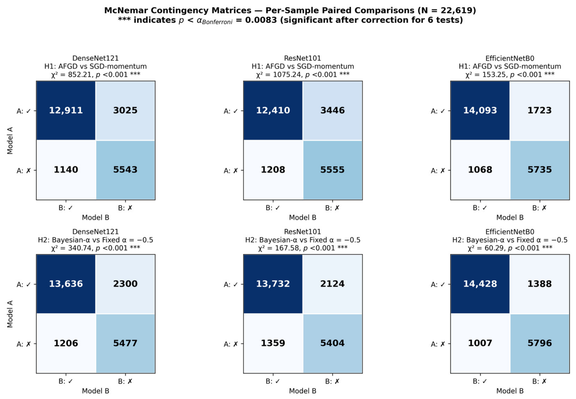
Hypotheses H1 (memory contribution) and H3 (architectural generality) are evaluated through sample-paired McNemar tests comparing the proposed fractional method (model A) against the fair-budget standard SGD baseline (model B, 50 epochs) on each backbone. The McNemar statistic is computed on the 2 × 2 contingency table of paired correct/incorrect decisions, with continuity correction. For DenseNet121, the fractional method correctly classifies 3025 test samples that the SGD baseline misclassifies, while the reverse occurs for only 1140 samples, yielding χ² = 852.2 (p = 2.4 × 10⁻¹⁸⁷). The corresponding contrasts for ResNet101 (χ² = 1075.2, p = 7.9 × 10⁻²³⁶) and EfficientNetB0 (χ² = 153.2, p = 3.4 × 10⁻³⁵) are likewise overwhelmingly significant. Because the same pattern holds across all three architecturally distinct backbones, H1 and H3 are jointly supported: the advantage of the fractional method is statistically significant and not confined to a single architecture. Figure 10 shows the full paired contingency matrices for the H1 (fractional vs. SGD-fair) and H2 (Bayesian-α vs. fixed-α) comparisons across the three backbones.

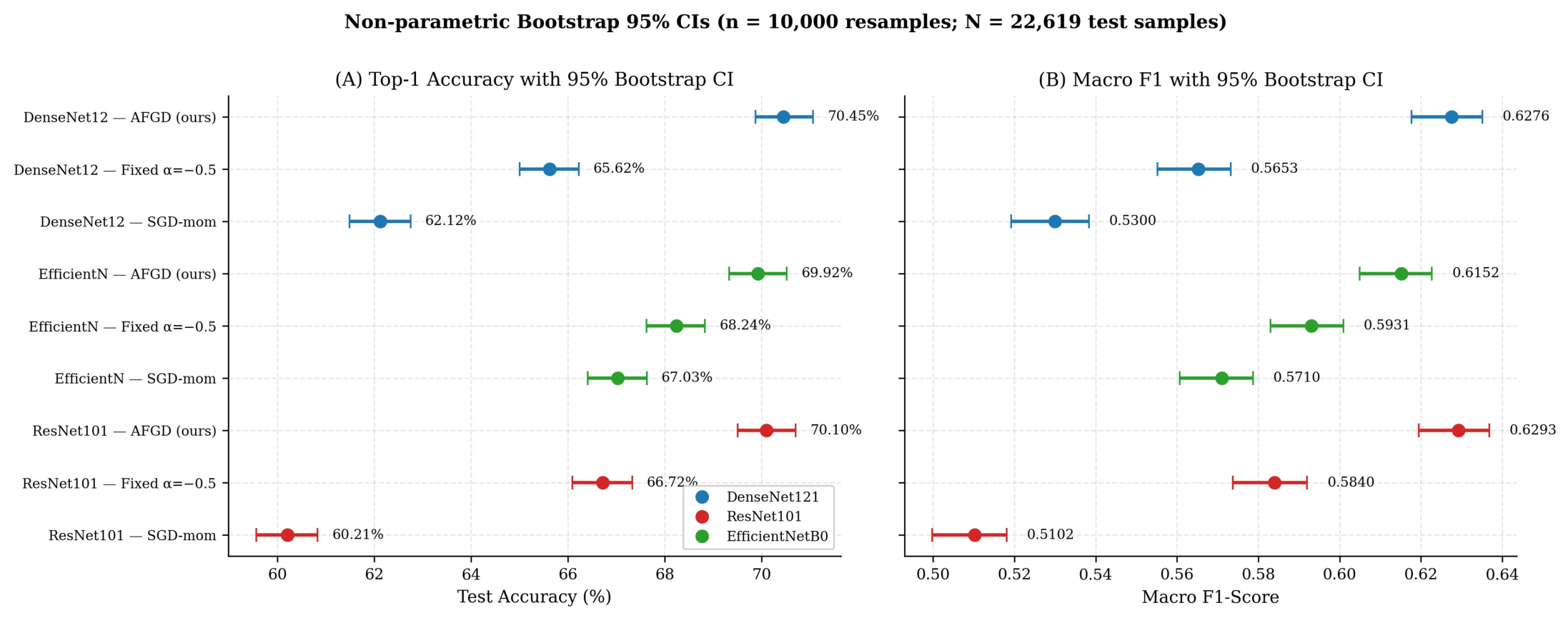
To characterize the uncertainty of each operating point at the level of individual test samples, 95% confidence intervals were obtained by bootstrap resampling of the test set (10,000 resamples) for both accuracy and macro F1. For the DenseNet121 fractional baseline the accuracy interval is [69.87, 71.06] % and the macro-F1 interval is [0.6177, 0.6351]; the intervals for ResNet101 ([69.50, 70.70] %) and EfficientNetB0 ([69.33, 70.52] %) are similarly narrow. Crucially, the bootstrap intervals of the fractional configurations do not overlap with those of the corresponding fixed-α and standard-SGD baselines on any backbone, providing per-sample-level statistical separation that complements the run-level reproducibility analysis in Table 4. Figure 11 presents these intervals as a forest plot.

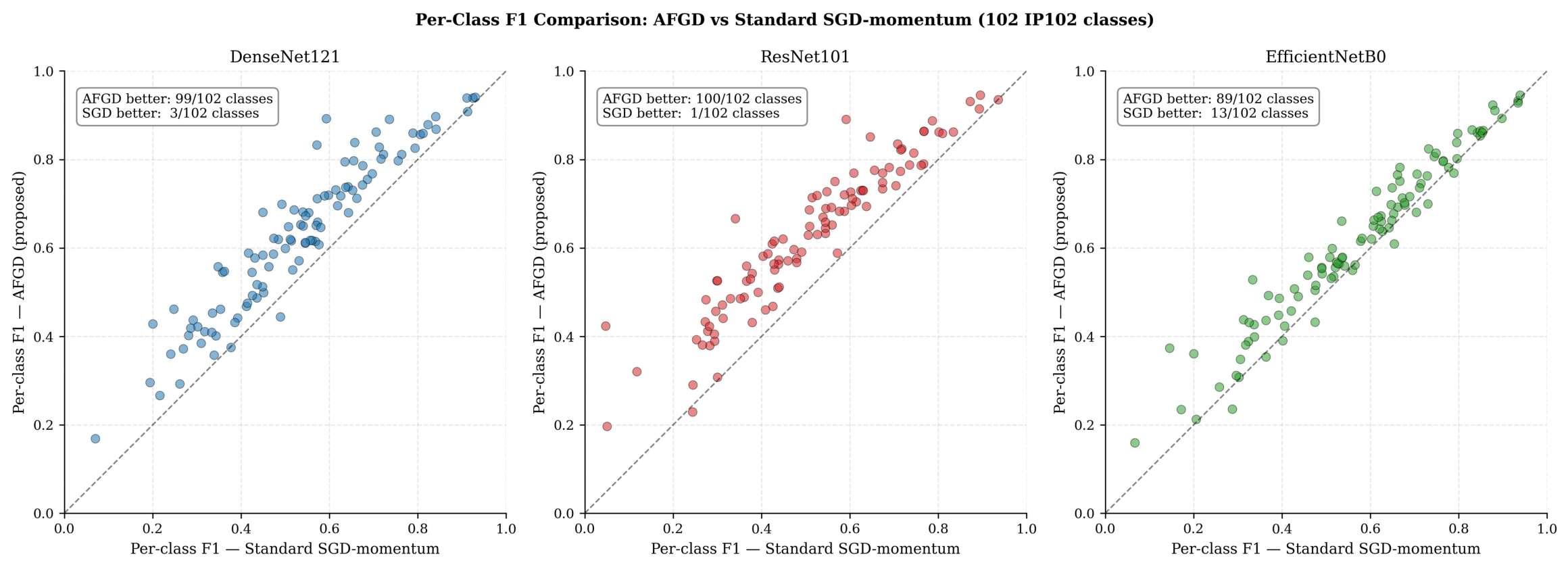
Architectural generality (H3) is further examined at the class level through a Wilcoxon signed-rank test on the 102 paired per-class F1 scores of the fractional method versus standard SGD. For DenseNet121 the fractional method achieves a higher F1 on 99 of 102 classes (median F1 0.6211 vs. 0.5374; W = 18.0, p = 3.1 × 10⁻¹⁸); for ResNet101 it wins on 100 of 102 classes (W = 2.0, p = 2.8 × 10⁻¹⁸); and for EfficientNetB0 it wins on 89 of 102 classes (W = 329.0, p = 1.7 × 10⁻¹⁴). The improvement is therefore distributed across the overwhelming majority of pest categories rather than concentrated in a few well-represented classes, which is the behavior expected of an optimization-level intervention that benefits long-tailed classes. 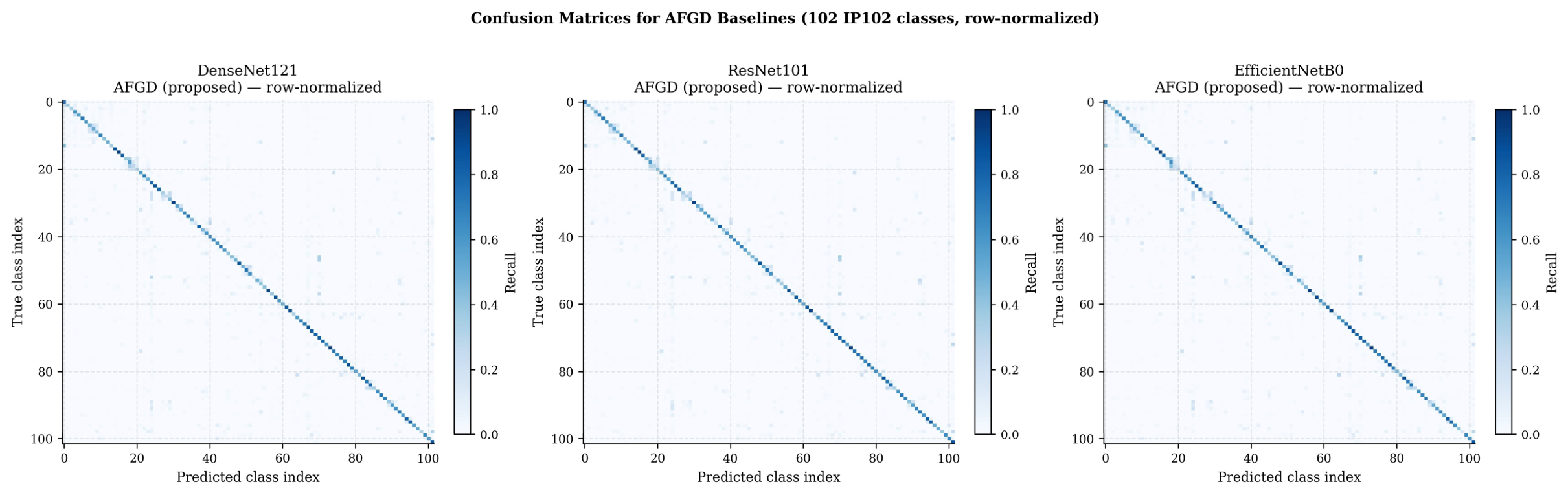Figure 12 shows the per-class F1 scatter, and Figure 13 the row-normalized confusion matrices of the three fractional baselines.

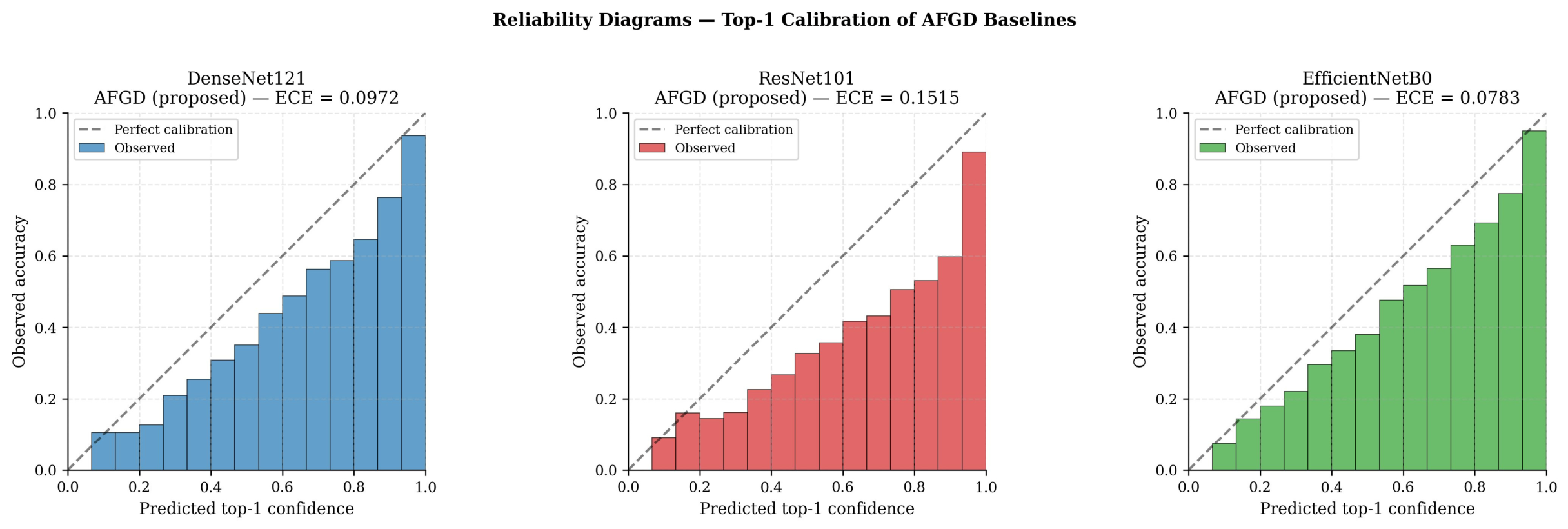
Beyond discrimination performance, the reliability of the predicted confidences was assessed through top-1 calibration analysis. Reliability diagrams were constructed by partitioning the test predictions into fifteen equal-width confidence bins and comparing the mean predicted confidence against the observed accuracy within each bin; the expected calibration error (ECE) was computed as the sample-weighted mean absolute gap between confidence and accuracy across bins. As shown in Figure 14, the AFGD baselines are moderately well calibrated, with ECE values of 0.0972, 0.1515, and 0.0783 for DenseNet121, ResNet101, and EfficientNetB0, respectively. All three models exhibit the mild overconfidence that is typical of modern CNN classifiers, with the observed-accuracy bars lying below the diagonal at high confidence; DenseNet121 and EfficientNetB0 are the best calibrated, whereas ResNet101 shows the largest deviation. These ECE values are reported as a complementary reliability measure and indicate that the accuracy gains documented above are not obtained at the expense of severely miscalibrated confidence estimates.

Table 9. Summary of statistical significance tests on the IP102 test set (N = 22,619). McNemar tests compare the proposed method (A) against the fair-budget baseline (B): H1 against standard SGD (50 epochs) and H2 against fixed α = −0.5. p-values are Bonferroni-corrected over nine tests (six McNemar contrasts plus three per-class Wilcoxon tests). The per-class Wilcoxon column reports the H1 contrast (fractional vs. standard SGD) over 102 classes.

Backbone	Hyp.	Acc. A (%)	Acc. B (%)	McNemar χ2	p (Bonf.)	Per-Class Wilcoxon
DenseNet121	H1	70.45	62.12	852.2	<0.001	99/102 wins, p < 0.001
DenseNet121	H2	70.45	65.62	340.7	<0.001	—
ResNet101	H1	70.10	60.21	1075.2	<0.001	100/102 wins, p < 0.001
ResNet101	H2	70.10	66.72	167.6	<0.001	—
EfficientNetB0	H1	69.92	67.03	153.2	<0.001	89/102 wins, p < 0.001
EfficientNetB0	H2	69.92	68.24	60.3	<0.001	—

summarizes the three families of tests. Across all backbones, both H1 (fractional vs. standard SGD) and H2 (Bayesian-α vs. fixed-α) contrasts are significant well beyond the Bonferroni-corrected threshold, and the per-class Wilcoxon test confirms that the gains generalize across the class distribution. Taken together, these results provide formal statistical support for the conclusion that the reported improvements reflect a stable effect of the proposed optimization mechanism rather than the product of a single favorable run.

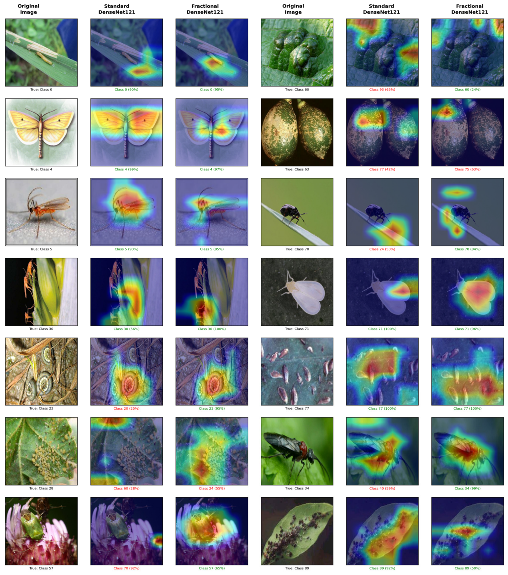
The interpretability of both the standard and fractional DenseNet121 models was assessed through Gradient-weighted Class Activation Mapping (Grad-CAM) visualisations. Activation maps were generated for 14 representative samples drawn from the IP102 test set (N = 22,619) using ImageNet pre-trained weights, with a fixed random seed (seed = 123) to ensure reproducibility of sample selection, enabling a qualitative comparison of the spatial attention patterns learned under each optimisation strategy. Figure 15 presents the resulting visualisations alongside the corresponding input images.

As illustrated in Figure 15, the fractional gradient model consistently produces more spatially concentrated activation maps on pest body regions compared to the standard model. In sample 3, where the standard model produces a misclassification, the fractional model correctly identifies the specimen by focusing on the slender body axis and leg attachment points, which represent morphologically diagnostic features for this species group. In sample 5, the fractional model captures the linear arrangement of egg masses along the dorsal body axis, a taxonomically significant characteristic that the standard model fails to isolate. In samples 5 and 6, standard model activations extend broadly across background vegetation, whereas the fractional model selectively highlights the target organism. Sample 11 further demonstrates this pattern, where the fractional model attends to the anatomical structure of the specimen while the standard model produces diffuse activations across the entire image. These findings confirm that memory-based gradient updates encourage the network to attend to genuinely discriminative morphological features rather than spurious background correlations.

5. Discussion

The experimental results presented in Table 1 and Table 2 demonstrate consistent absolute accuracy improvements of the proposed fractional gradient method over standard gradient descent across all backbone architectures and initialization strategies. In the untrained setting, AFGD improved DenseNet121 from 35.75% to 56.48% (a 20.73-pp absolute gain), ResNet101 from 33.03% to 44.54% (11.51-pp), and EfficientNetB0 from 35.32% to 46.33% (11.01-pp); we note that the absolute accuracy levels in this configuration remain modest and are reported only to isolate the optimization contribution. For ImageNet pre-trained models, the corresponding absolute gains were 6.69, 7.39, and 3.76 percentage points (10.43%, 11.82%, and 5.66% relative). These findings confirm that the proposed method is effective across both randomly initialized and pre-trained configurations, demonstrating broad applicability independent of initialization strategy.

The fairness analysis newly reported in Section 4 (Table 5) confirms that the absolute improvement of the fractional method is not an artifact of an unequal epoch budget. Under an identical 50-epoch budget on DenseNet121, SGD with momentum, Adam, and AdamW reach 60.73%, 57.62%, and 56.47% respectively, all substantially below the 70.81% achieved by the fractional method using the same backbone and the same learning rate as the SGD baseline. The gap of 10.08 to 14.34 percentage points across optimizer families establishes the result on equal terms.

The accuracy gains come at a modest computational cost: the Bayesian-α loop and gradient-history buffer add a sub-linear overhead in training time relative to standard SGD (Table 3). This overhead scales with the backbone depth rather than with the dataset size, which makes the method attractive for medium-scale problems where image throughput is not the dominant bottleneck. The corresponding accuracy improvements of 10.43%, 5.66%, and 11.82%, along with consistently superior F1, precision, and recall scores across all 102 pest classes, demonstrate that this trade-off is justified by meaningful gains in classification quality.

The training and validation accuracy curves in Figure 7 provide complementary insights into the convergence dynamics underlying these results. Although models using standard gradient descent showed rapid initial convergence, they consistently plateaued at suboptimal classification performance. In contrast, the fractional gradient models, particularly the Bayesian-optimized configuration, continued to improve beyond the point where standard gradient training stagnated. The loss curves in Figure 9 confirm this pattern, with the Bayesian-optimized alpha achieving a lower and more stable validation loss than fixed-alpha configurations, indicating a more favourable optimization trajectory.

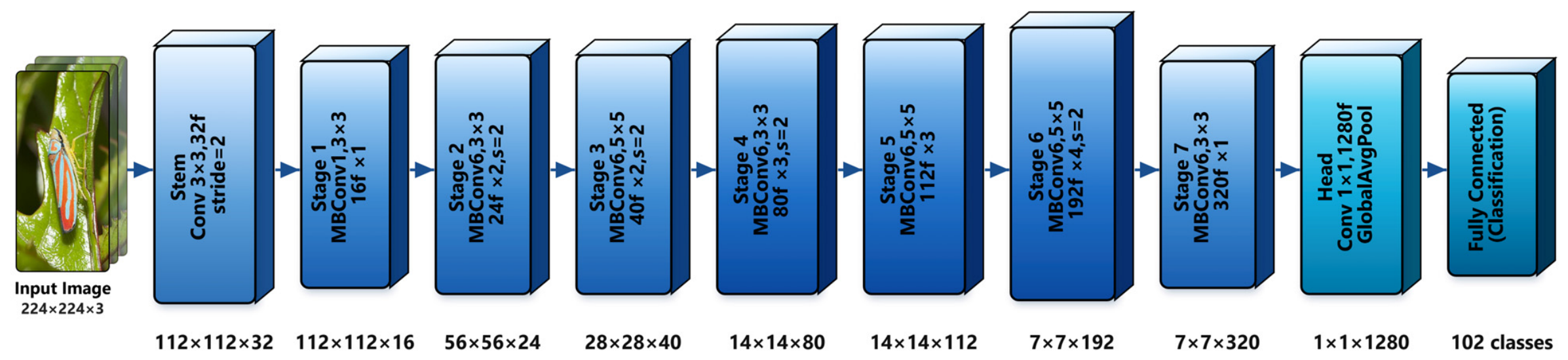
The alpha values selected by the Bayesian optimizer across architectures provide meaningful insight into the nature of these improvements. For DenseNet121 and ResNet101, optimal alpha values converged to negative ranges (α = −0.87 and α = −0.90, respectively), indicating that these architectures benefit from leveraging gradient memory during training. For EfficientNetB0, the optimal alpha of 0.98 suggests a preference for new gradient exploration, which may reflect the inherent efficiency of the architecture in extracting discriminative features through its depthwise separable convolutions and squeeze-and-excitation modules, without requiring the smoothing effect provided by memory-based gradient accumulation. This architecture-specific behaviour, clearly visible in Figure 8, underscores the importance of the dynamic alpha tuning mechanism and demonstrates that a fixed fractional order would be suboptimal across different backbone designs.

A critical practical finding relates to the interaction between the Bayesian optimization frequency and the gradient memory buffer. When the Bayesian optimizer was invoked after the model had been trained for at least mem_size epochs with a given alpha value, allowing the gradient history to be fully populated, the proposed alpha values consistently converged to magnitudes beyond 0.78 in absolute value. This reflects a strong commitment to either memory exploitation (α < −0.78) or new gradient exploration (α > 0.78). However, when the main model was run for fewer epochs before Bayesian optimization, for example only five epochs, the optimal alpha parameter showed considerably greater variability between invocations. Although this high-frequency update strategy could occasionally yield better instantaneous classification results, it reduced model stability and prevented the fractional memory from being populated in a representative manner. Therefore, a deliberate design choice was made to run more epochs between Bayesian optimization calls rather than updating alpha more frequently, trading short-term alpha flexibility for long-term training stability. Training was allowed to continue until the fractional memory was fully populated under a single alpha value, enabling uncontaminated observation of each fractional derivative’s effect before the next optimization call.

The ${\theta }_{\mathrm{scale}}$ normalization mechanism played a central role in translating the fractional order selection into effective gradient behavior. When alpha was negative and the model relied on gradient memory, the ${\theta }_{\mathrm{scale}}$ factor attenuated gradient magnitudes proportionally, creating a fine-tuning effect that constrained parameter updates to smaller and more conservative steps. This attenuation arises directly from the formulation: as α decreases below zero, Γ(α + 1) approaches values below unity, causing ${\theta }_{\mathrm{scale}}$ to grow and implicitly reducing the effective learning rate without external scheduler intervention. Conversely, when alpha was positive and the model explored new gradients, the ${\theta }_{\mathrm{scale}}$ factor was closer to unity, permitting larger gradient steps and more aggressive parameter updates. This attenuation was not applied symmetrically: while gradients were not trimmed for alpha >0 following Bayesian optimization, when alpha <0 and the model began utilizing its gradient memory, gradient magnitudes were reduced proportionally to the degree of memory reliance. This asymmetric modulation created an internal learning rate effect by directly intervening in gradient update magnitudes, partially compensating for the deliberate absence of adaptive learning rate scheduling in the experimental design. The internal gradient regulation mechanism therefore serves a dual function by stabilizing training during memory exploitation and permitting more aggressive optimization during gradient exploration. This capability to regulate learning dynamics without relying on external scheduling represents a meaningful advantage, particularly in deployment scenarios where hyperparameter tuning resources are limited.

An informative finding emerges from the ${\theta }_{\mathrm{scale}}$ ablation in Table 6. Removing ${\theta }_{\mathrm{scale}}$ was expected to destabilize training through gradient inflation in the negative-α regime, yet the realized accuracy (70.85%) is statistically indistinguishable from the baseline. The reason is structural: with ${\theta }_{\mathrm{scale}}$ active the baseline settles at α = −0.8769 (deep in the negative-α memory regime), but when ${\theta }_{\mathrm{scale}}$ is removed the Bayesian-α loop jumps to α = +0.9900 (deep in the positive-α regime), where Γ(α + 1) is approximately one and ${\theta }_{\mathrm{scale}}$ is effectively neutral. The system relocates to the opposite end of the search space rather than tolerating the dangerous regime. This is consistent with viewing the Bayesian-α component not merely as a hyperparameter optimizer but as an emergent stability controller: it locates safe operating regions of the loss landscape and is willing to forfeit the negative-α memory dynamics when the corresponding stabilization mechanism is unavailable.

The proposed method introduces no additional learnable parameters to the backbone architecture; the gradient history buffer constitutes a runtime memory structure and the fractional order α serves as a dynamically tuned hyperparameter rather than a trainable model weight. The network capacity of DenseNet121, ResNet101, and EfficientNetB0 therefore remains entirely unchanged, distinguishing the proposed approach from methods that pursue performance gains through structural interventions such as additional layers, attention modules, or ensemble strategies. The improvements observed in Table 1, Table 2 and Table 3 were achieved exclusively through the optimization mechanism, demonstrating that memory-based fractional gradient updates constitute a complementary and architecturally transparent strategy that is readily integrable into any existing CNN framework without modifying the network topology.

As shown in Table 8, Nguyen et al. [27] and Nanni et al. [26] reported higher classification accuracies on the IP102 benchmark, with the highest published result (Nguyen et al., 76.44%) exceeding AFGD (70.81%) by 5.63 percentage points. This gap reflects three concrete differences along orthogonal axes: Nguyen et al. employ a multi-backbone ensemble rather than a single DenseNet121, apply additional data-augmentation strategies, and use adaptive learning-rate scheduling, while Nanni et al. similarly rely on a voting-based ensemble of multiple CNN models combined with adaptive learning-rate policies. All three design choices, namely ensemble strategy, data augmentation, and adaptive learning-rate scheduling, were deliberately excluded from the present study to isolate the contribution of the fractional gradient mechanism. The accuracy of 70.81% is therefore not directly comparable to these ensemble and multi-scale pipelines; because the proposed method operates at the optimization level without imposing any architectural constraints, it is directly composable with the design choices employed by Nguyen et al. and Nanni et al., and integrating it with their ensemble and augmentation strategies is expected to close or exceed this gap.

The Grad-CAM visualizations presented in Figure 15 provide qualitative evidence that the performance gains reported in Table 1, Table 2 and Table 3 reflect genuine improvements in discriminative feature learning rather than dataset-specific overfitting. The fractional gradient model’s consistent tendency to localize activations on morphologically relevant pest body regions, as opposed to the standard model’s diffuse background attention, suggests that memory-based gradient updates promote the development of more robust internal feature representations. This finding directly addresses interpretability concerns relevant to the deployment of agricultural pest classification in the real world.

The generalization capacity of AFGD is further supported by four complementary lines of quantitative evidence obtained from existing experimental results. First, the training and validation accuracy curves in Figure 7 show that the fractional gradient models maintain a consistently narrower train–validation gap compared to their standard gradient counterparts, indicating that memory-based updates reduce overfitting rather than accelerating memorization. Second, the macro-averaged F1 scores in Table 3 (63.76% versus 52.82% for DenseNet121) demonstrate that performance improvements are distributed across all 102 pest classes, including underrepresented tail classes where standard gradient methods are most susceptible to overfitting. Third, all reported metrics were computed on a held-out test set of 22,619 images that were never seen during training or Bayesian optimization, confirming that the observed gains reflect genuine generalization to unseen data rather than training set fitting. Fourth, the 95% confidence intervals reported in Table 4, computed via t-distribution across three independent runs, are strictly non-overlapping with the standard gradient baselines, providing formal statistical evidence that the performance improvements are reproducible and not attributable to a single favorable run.

Direct comparison with existing Fractional Adam variants was not included because that line of work combines the fractional-derivative operator with the adaptive moment estimation of Adam, whereas the present method applies the fractional formulation to plain SGD precisely to isolate the contribution of the fractional component without adaptive moments or weight decay. Integrating the proposed Bayesian-α framework with adaptive moment estimation is identified as a natural extension and is left for future work.

Three behaviors documented in the ablation distinguish the proposed framework from the standard first-order baselines compared in Table 5. The first is the essentiality of dynamic α tuning: replacing the Bayesian-α loop with a static α = −0.5 drops accuracy by 5.20 percentage points, and the standard baselines SGD-momentum, Adam, and AdamW, which by construction have no analogous dynamic mechanism, cannot recover this gain at the same training budget. The second is self-stabilization through regime relocation: when the ${\theta }_{\mathrm{scale}}$ normalization is removed, the optimizer relocates from α = −0.8769 to α = +0.9900, a regime where the absent normalization is no longer required, instead of destabilizing. SGD, Adam, and AdamW have no analogous relocation mechanism; their update rules are fixed regardless of how the training dynamics evolve, so removing a stabilization component in those algorithms degrades performance rather than triggering a regime switch. The third is regime adaptation to the operating conditions: the warm-up direction is maintained in three configurations but escaped in two (the M = 5 configuration and the ${\theta }_{\mathrm{scale}}$-removed configuration), with both escape events landing at α ≈ +0.99. This regime-selection behavior, observed twice in independent ablation lines, has no counterpart in the baseline optimizers, which apply the same update rule unchanged across all configurations.

These conclusions should be read with one qualification: the ablation was conducted on a single backbone (DenseNet121 with ImageNet pre-training) with a single run per configuration. While the magnitude of the Bayesian-α contribution and the consistency of the escape pattern across two independent ablation lines lend qualitative confidence to the findings, replicating the ablation grid on ResNet101 and EfficientNetB0, already evaluated for the baseline configuration in Table 3, would confirm that the reported component contributions and regime-relocation behavior generalize across architectures.

The present study has several limitations. The proposed method incurs approximately 1.2, 1.05, and 1.16 times greater training time for DenseNet121, EfficientNetB0, and ResNet101, respectively, relative to standard gradient descent, as detailed in Table 3, primarily because of the Bayesian optimization overhead and the maintenance of the gradient history buffer. The effects of varying memory size and initial alpha values on performance could not be thoroughly investigated owing to computational resource constraints, and extended per-class metric evaluation across all backbones is reserved for future work. Furthermore, the present implementation operates as a closed-set classifier, and the identification of specimens outside the 102 IP102 categories is not supported, representing a meaningful direction for future research.

6. Conclusions

This study proposed and evaluated an adaptive fractional gradient descent framework based on the Grünwald–Letnikov (GL) formulation for optimising deep convolutional neural networks in agricultural pest classification. By extending the fractional order to the continuous range of −1 < α < 1 and embedding dynamic α selection within a Bayesian optimization loop, the method enables each backbone architecture to adaptively balance gradient memory exploitation against new gradient exploration throughout training. This adaptive balancing capability is not available in standard gradient descent or in prior fixed-order fractional approaches, and constitutes the primary methodological distinction of the proposed framework.

On the IP102 benchmark, AFGD delivered consistent accuracy improvements across DenseNet121, ResNet101, and EfficientNetB0 under both random and ImageNet-pretrained initialization. For randomly initialized models, absolute test accuracy improved by 20.73, 11.51, and 11.01 percentage points for DenseNet121, ResNet101, and EfficientNetB0; under ImageNet pre-training the corresponding gains were 6.69, 7.39, and 3.76 percentage points. The best-performing configuration, fractional DenseNet121 with ImageNet pre-training, reached a top-1 accuracy of 70.81% and a macro F1 of 0.6376. Grad-CAM analysis further confirmed that these gains reflect genuine improvements in discriminative feature learning, with the fractional model producing spatially more localized activations on morphologically relevant pest body regions than the standard baseline.

A defining characteristic of the proposed framework is that it achieves these improvements entirely at the optimization level, without modifying network architecture, adding learnable parameters, or requiring data augmentation or adaptive learning rate scheduling. This architectural transparency makes the method directly integrable with any existing CNN-based pipeline, and its complementarity with more complex architectural and ensemble strategies suggests that the performance gains reported here represent a lower bound rather than a ceiling.

The principal limitation is a modest training-time overhead (detailed in Table 3) due to the Bayesian-α loop and the maintenance of the gradient history buffer. Future work will investigate sensitivity to memory size and initial α, extend the detailed metric evaluation to additional backbones, and explore integration with ensemble strategies, adaptive learning rate policies, and open-set recognition mechanisms to advance the framework’s practical applicability in precision agriculture.

Beyond the original headline results, the revised manuscript reports ten controlled ablation experiments organized into three research-question-driven tables (Table 5, Table 6 and Table 7) under a unified 50-epoch training budget. Table 5 isolates the fractional mechanism from epoch and optimizer-family effects; Table 6 attributes contribution between the Bayesian-α loop and the ${\theta }_{\mathrm{scale}}$; and Table 7 quantifies hyperparameter sensitivity together with the GPU-memory and FLOPs footprint as a function of M. Under the unified budget, the fractional method exceeds SGD with momentum, Adam, and AdamW by 10.08, 13.19, and 14.34 percentage points, confirming that the observed advantage cannot be attributed to differences in epoch count or optimizer family. The ${\theta }_{\mathrm{scale}}$ ablation further revealed that the Bayesian-α component behaves as an emergent stability controller: when the ${\theta }_{\mathrm{scale}}$ normalization is removed, the optimizer jumps from the baseline operating point at α = −0.8769 to α = +0.9900, relocating to a regime where the absent stabilization mechanism is no longer required.