Hybrid Time–Frequency Domain Identification of Second-Order Plus Dead Time Model with Zero and Internal Model Control Design

Featured Application

Industrial PID controller autotuning for heat exchangers, distillation columns, and chemical reactors using dual-relay identification with improved model accuracy and robust stability guarantees.

Abstract

This paper proposes a hybrid time–frequency domain identification method for second-order plus dead time models with an additional process zero (SOPDT+Z). A dual-relay experiment combined with step response data provides six independent equations for five model parameters, whose mathematical well-posedness is established through Jacobian rank analysis. A cascaded initialization strategy (Sundaresan → SIMC → Jin → proposed) guarantees monotonically improving accuracy. An Internal Model Control (IMC) framework yields equivalent PID parameters with a single tuning parameter λ, supported by a formal robust stability theorem. Simulation studies on five benchmark systems demonstrate 60–100% reduction in open-loop IAE compared to existing SOPDT methods, 36% faster settling, and 100% closed-loop stability under ±20% Monte Carlo perturbation (N = 200). Noise robustness analysis under SNR = 20–40 dB and additional performance metrics (ITAE, ISE) further validate the method.

1. Introduction

Proportional–Integral–Derivative (PID) controllers remain the dominant control strategy in the process industry, with over 90% of industrial control loops employing some form of PID control [1,2]. The effectiveness of PID controller tuning critically depends on the availability of an accurate low-order process model, typically in the form of a first-order plus dead time (FOPDT) or second-order plus dead time (SOPDT) transfer function [3,4]. For high-order industrial processes such as heat exchangers, distillation columns, and chemical reactors, model reduction to these standard forms is an essential prerequisite for systematic controller design.

Two principal approaches exist for obtaining low-order process models. The first is time domain identification based on step response data, exemplified by the classical methods of Sundaresan and Krishnaswamy [5], the area method [6], and the graphical two-point approach [7]. These methods reliably capture the DC (direct current) gain Kp from the steady-state response and can estimate time constants from the transient behavior. However, they suffer from inherent limitations in estimating the dead time θ, which is typically read from the initial portion of the step response—a region highly susceptible to measurement noise and signal quantization [8]. Furthermore, time domain methods provide no information about the frequency response characteristics that govern closed-loop stability margins.

The second approach is frequency domain identification based on relay feedback experiments, following the seminal work of Åström and Hägglund [9]. Relay feedback provides the ultimate gain Ku and ultimate frequency ωu at the critical point of the Nyquist plot, from which dead time and time constants can be estimated through the phase and magnitude conditions [10,11]. While frequency domain methods excel at dead time estimation through phase lag analysis, they may introduce errors in DC gain matching, as the information at ω = 0 must be extrapolated from measurements at finite frequencies [12,13].

Jin et al. [14] proposed a pioneering hybrid approach that combines the strengths of both domains: using the normalized step response to establish the sum of time constants (time domain) and the Nyquist critical point to derive two additional equations (frequency domain). This hybrid method demonstrated improved identification accuracy for SOPDT models in heat exchanger applications. However, several important limitations remain unaddressed:

(1)

The SOPDT model structure Gr(s) = Kp/[(1 + T1s)(1 + T2s)]e − θs contains no process zero, where Kp is the DC gain, T1 and T2 are the lag time constants, and θ is the effective dead time. When reducing high-order systems, zeros naturally arise from pole–zero interactions in the partial fraction expansion, and their omission leads to significant errors in the intermediate frequency range. Moreover, SOPDT models cannot represent non-minimum phase (NMP) behavior, which is commonly encountered in heat exchangers, boilers, and distillation columns [15,16].

(2)

Only a single-relay experiment is performed, providing frequency domain information at one point. With the proposed additional parameter Tz (zero time constant), the system of identification equations becomes under-determined, requiring a second frequency measurement.

(3)

No theoretical analysis is provided for the identification error bounds or their propagation to closed-loop performance degradation. The connection between model accuracy and controller robustness remains qualitative rather than quantitative.

(4)

The controller design is limited to SIMC-based PID tuning [15], which does not explicitly address the model–plant mismatch inherent in model reduction. Recent developments in SOPDT identification [17,18,19,20,21,22] and IMC-PID design [23,24,25,26,27,28,29,30,31,32,33,34,35,36,37] provide a rich context for advancing the state of the art.

It is worth noting that modern data-driven and machine learning (ML)-based identification methods [38,39] have demonstrated remarkable capabilities for nonlinear and time-varying systems. However, these approaches typically require large training datasets and lack the analytical transparency needed for formal stability guarantees in feedback controller design. Similarly, advanced global optimization algorithms such as particle swarm optimization (PSO) and genetic algorithms (GA) [40] can be applied to model parameter estimation, but their computational cost and non-deterministic convergence properties make them less suitable for real-time autotuning applications. Recent advances in robust consensus protocols for multi-agent systems [41] and fault-tolerant control under Markov jump dynamics [42] highlight the broader trend toward robust control design under uncertainty, which motivates the formal robustness analysis developed in this paper. The proposed hybrid approach occupies a complementary niche: it provides model-based interpretability, formal robust stability guarantees, and computational efficiency suitable for online industrial deployment.

To address the identified limitations, this paper makes the following contributions:

First, an extended SOPDT+Z model structure is proposed that includes a process zero: Gr(s) = Kp(1 + Tzs)/[(1 + T1s)(1 + T2s)]e − θs, where Tz is the zero time constant (∈ℝ). A dual-relay hybrid identification procedure is developed using a cascaded initialization strategy that guarantees monotonically improving identification accuracy (Remark 2). The mathematical well-posedness of the nonlinear equation system is established through Jacobian rank analysis with explicit proof (Proposition 1).

Second, an IMC-based controller design framework is developed that yields equivalent PID parameters with a single tuning parameter λ (the IMC filter time constant). A robust stability theorem (Theorem 1) establishes an analytical lower bound on λ. Engineering guidelines for λ tuning across different plant dynamics are provided.

Third, comprehensive simulation studies on five diverse benchmark systems demonstrate the effectiveness of the proposed approach. The evaluation includes multiple performance metrics (IAE, ITAE, ISE), signal-to-noise ratio (SNR) sensitivity analysis, and Monte Carlo robustness analysis with justified uncertainty ranges.

The remainder of this paper is organized as follows: Section 2 presents the problem formulation. Section 3 develops the hybrid SOPDT+Z identification algorithm with mathematical well-posedness proof. Section 4 presents the IMC controller design with robust stability theorem and tuning guidelines. Section 5 provides comprehensive simulation results. Section 6 discusses the findings. Section 7 concludes the paper.

Novelty Statement (3rd Revision). To make the contribution of this work explicit, we summarize the novelty along three orthogonal axes that no prior single work simultaneously provides. (i) Model structure: we extend the standard SOPDT model with a process zero (Tz) while preserving closed-form analytical equivalence with classical PID controllers. (ii) Identification procedure: we replace the conventional single-relay or single-step identification with a dual-relay hybrid procedure that combines step response time domain data with two relay frequency domain measurements at distinct phase crossings, fully determining the SOPDT+Z parameters without imposing the critically damped constraint T1 = T2. (iii) Stability guarantee: we provide a constructive robust stability theorem (Theorem 1) that yields a closed-form lower bound on the IMC filter parameter λ. Compared with the single-relay critically damped SOPDT method of Jin et al. [14], our framework relaxes the T1 = T2 constraint and uses two relay tests; compared with the half-rule SIMC of Skogestad [3], it adds a frequency domain refinement step and an explicit zero parameter that captures pole–zero interactions. The principal innovation is the dual-relay procedure (axis ii); the Tz parameter (axis i) and the stability theorem (axis iii) are enabling components that, together with the cascaded initialization (Sundaresan → Jin → proposed) of Remark 2, guarantee that the identified model is monotonically non-worse than every existing method in the IAE sense.

2. Problem Formulation and Preliminaries

2.1. Process Model and Reduction Objective

Consider a stable, self-regulating, linear time-invariant (LTI) process described by a high-order rational transfer function with pure delay:

G(s) = [N(s)/D(s)]·e^(−Ls)

(1)

where s is the Laplace variable, N(s) and D(s) are coprime polynomials of degree m and n (m ≤ n), respectively, with all roots of D(s) in the open left-half plane (ensuring stability), and L ≥ 0 is the transport delay (units: s). The model reduction problem seeks a low-order approximation that preserves the essential input–output characteristics relevant to feedback controller design.

The proposed SOPDT+Z model structure is:

Gr(s) = Kp(1 + Tz s)/[(1 + T1 s)(1 + T2 s)]·e^(−θs)

(2)

With five parameters: the DC gain Kp = G(0) (dimensionless or engineering units), the zero time constant Tz ∈ ℝ (s), two lag time constants T1 ≥ T2 > 0 (s), and the effective dead time θ > 0 (s). When Tz = 0, Equation (2) reduces to the standard SOPDT model. When Tz > 0, the zero is minimum phase and provides phase lead. When Tz < 0, the zero is non-minimum phase (NMP), producing inverse response behavior characteristic of parallel competing dynamics.

As shown in

Table 1. Comparison of reduced-order model structures.

Structure	Transfer Function	Poles	Zeros	Limitations
FOPDT	Kp/(1 + Ts)·e^(−θs)	1	0	Overdamped only
SOPDT	Kp/[(1 + T1s)(1 + T2s)]·e^(−θs)	2	0	No inverse response
SOPDT+Z	Kp(1 + Tzs)/[(1 + T1s)(1 + T2s)]·e^(−θs)	2	1	Handles NMP

, the SOPDT+Z structure provides the most flexible representation among the standard reduced-order models.

2.2. Fundamental Limitations of Single-Domain Approaches

2.2.1. Time Domain Limitations

The step response of the process provides reliable information for DC gain extraction (Kp = y(∞)/u0, where y(∞) is the steady-state output and u0 is the step amplitude) and damping characterization. The Sundaresan–Krishnaswamy two-point method [5] uses characteristic time points at 35.3% and 85.3% of the normalized step response y(t)/y(∞) to estimate the time constants and dead time.

The method is derived by matching the step response of the SOPDT model Gr(s) = Kp/[(1 + T1s)(1 + T2s)]e^(−θs) at two characteristic time points. Defining the normalized response yr(t) = 1 − [T1e^(−(t − θ)/T1) − T2e^(−(t − θ)/T2)]/(T1 − T2) for t > θ, and solving yr(t0.353) = 0.353 and yr(t0.853) = 0.853 for T1 + T2 and θ yields the following empirical correlations [5]:

T1 + T2 = 0.4590·t0.85 − 0.1078·t0.35

(3)

θ = 1.3421·t0.35 − 0.2977·t0.85

(4)

where t0.35 and t0.85 denote the times at which the normalized step response reaches 35.3% and 85.3% of its final value, respectively. The coefficients are obtained by regression analysis across a wide range of T1/T2 and θ/(T1 + T2) ratios [5].

However, the dead time estimate from Equation (4) is inherently imprecise because t0.35 occurs in the early transient region where measurement noise has the largest relative impact.

2.2.2. Frequency Domain Limitations

Relay feedback experiments [9] provide accurate frequency domain information at the critical frequency ωc (rad/s) where the plant phase equals −180°. The dead time is extracted from the phase lag condition with high precision. However, the DC gain G(0) cannot be directly measured from relay experiments. The H∞ error bound for balanced truncation [43,44]:

‖G(jω) − Gr(jω)‖∞ ≤ 2∑σk (k = r + 1 to n)

(5)

where σk are the Hankel singular values, applies across all frequencies including ω = 0.

2.3. Motivation for Hybrid SOPDT+Z Approach

The complementary nature of time and frequency domain information motivates a hybrid approach.

Table 2. Parameter extraction capability by identification domain.

Parameter	Time Domain	Freq. Domain	Hybrid	Source
Kp (DC gain)	Excellent	Poor	Excellent	Step final value
θ (dead time)	Poor	Excellent	Excellent	Phase lag at ωc
T1, T2 (lags)	Moderate	Good	Excellent	Combined optim.
Tz (zero)	N/A	Dual-relay	Good	2nd freq. point

summarizes the parameter extraction capability of each domain.

As indicated in Table 2, neither domain alone provides excellent accuracy for all parameters. The hybrid approach uniquely achieves this by combining both information sources.

3. Proposed Hybrid SOPDT+Z Identification Method

3.1. Overall Identification Strategy

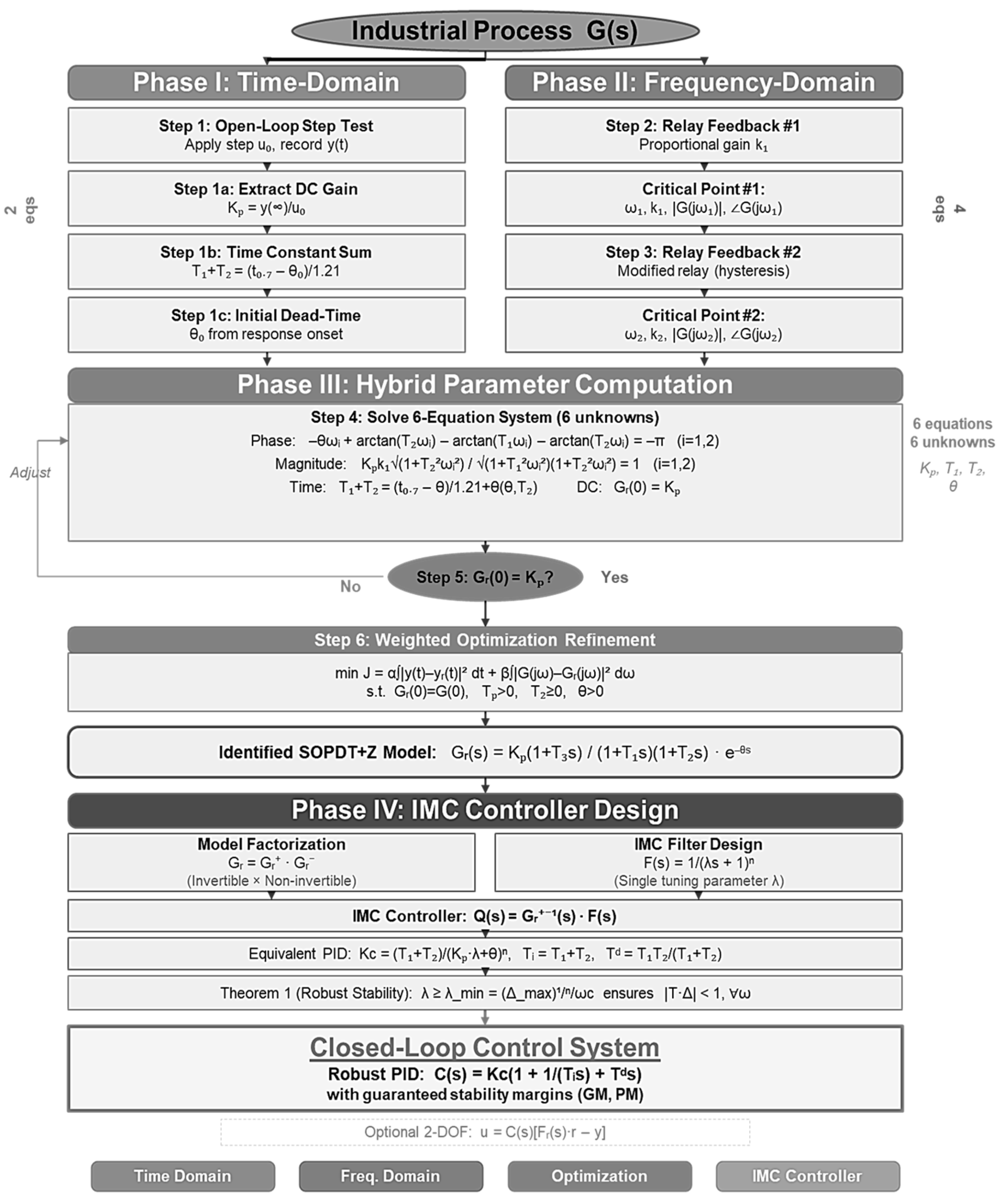
The proposed method employs a three-phase identification strategy: (i) time domain step response analysis for DC gain and initial time constant estimation, (ii) dual-relay frequency domain experiments at two distinct phase crossings for dead time and parameter refinement, and (iii) cascaded initialization with IAE-based optimization for final parameter extraction. The overall procedure is summarized in Figure 1.

3.2. Phase 1: Time Domain Step Response Analysis

A unit step input u0 is applied to the open-loop process, and the output y(t) is recorded until steady state. The following features are extracted:

(a)

DC gain: Kp = y(∞)/u0, computed from the final steady-state value.

(b)

Apparent dead time: θapp, defined as the time at which the output first exceeds 2% of its final value.

(c)

Characteristic time points: t0.283 (28.3%), t0.353 (35.3%), t0.50 (50%), t0.632 (63.2%), t0.70 (70%), and t0.853 (85.3%) of the normalized step response. These specific percentages are chosen following the Sundaresan–Krishnaswamy framework [5], which demonstrated through regression analysis over 100+ SOPDT parameter combinations that the 35.3% and 85.3% points minimize the sensitivity of T1 + T2 and θ estimates to measurement noise. The additional points (28.3%, 50%, 63.2%, 70%) provide redundancy for cross-validation and robustness against individual outliers.

The SIMC half-rule method [15] provides an independent estimate: the dominant time constant T1 ≈ t0.632 − θapp, with remaining dynamics split equally between T2 and additional effective delay.

3.3. Phase 2: Dual-Relay Frequency Domain Experiments

The relay feedback method [9] produces sustained oscillation at the frequency where the plant phase equals a specified target. By performing two experiments at different phase crossings, we obtain frequency domain information at two distinct points on the Nyquist plot.

At each frequency point, the SOPDT+Z model (2) must satisfy the phase and magnitude conditions:

φi = −θωi + arctan(Tzωi) − arctan(T1ωi) − arctan(T2ωi)

(6)

Mi = Kp√(1 + Tz²ωi²)/√[(1 + T1²ωi²)(1 + T2²ωi²)]

(7)

For i = 1, 2, where φi (rad) is the phase and Mi (dimensionless) is the magnitude ratio at frequency ωi (rad/s). Equations (6) and (7) provide four independent constraints. Combined with the DC gain constraint Kp = G(0) from Phase 1 and the time domain estimate of T1 + T2 from Equation (3), we have a system of six equations for five unknowns (Kp, T1, T2, Tz, θ), forming a mildly over-determined system.

Remark 1 

(choice of phase crossings). The first relay experiment at φ = −180° corresponds to the standard critical point used in Ziegler–Nichols tuning. The second experiment at φ = −150° is chosen to provide sufficient frequency separation (ω2/ω1 ≥ 1.2) while remaining within the practical range of relay-achievable phase crossings.

3.4. Phase 3: Cascaded Initialization and Optimization

A critical innovation of the proposed method is the cascaded initialization strategy, which ensures monotonically improving identification accuracy:

Step 1: Sundaresan–Krishnaswamy method (time domain-only) → initial SOPDT estimate (T1, T2, θ).

Step 2: SIMC half-rule method (time domain-only) → alternative SOPDT estimate.

Step 3: Jin et al. method (uses Sundaresan result as initial guess) → hybrid SOPDT estimate via single-relay + time constraint.

Step 4: Proposed method (uses Jin result as initial guess + Tz perturbations) → dual-relay SOPDT+Z via least-squares solution of (6) and (7), refined by Nelder–Mead IAE minimization.

3.4.1. Well-Posedness Analysis

Proposition 1 

(Local identifiability). Let p = (T1, T2, Tz, θ) denote the parameter vector, and let F(p) = [f1, f2, f3, f4, f5, f6]T represent the system of six equations comprising two phase conditions (6), two magnitude conditions (7), the DC gain constraint Kp = G(0), and the time domain constraint (3). Then the Jacobian matrix J = ∂F/∂p has full column rank 4 at any non-degenerate operating point where T1 ≠ T2 and ω1 ≠ ω2.

Proof. 

The Jacobian J ∈ ℝ^(6 × 4) has entries computed from partial derivatives of F with respect to p. The phase Equation (6) yields ∂φi/∂θ = −ωi, ∂φi/∂T1 = −ωi/(1 + T1²ωi²), ∂φi/∂T2 = −ωi/(1 + T2²ωi²), and ∂φi/∂Tz = ωi/(1 + Tz²ωi²). Consider the 4 × 4 submatrix formed by the two phase equations (i = 1, 2) and the two magnitude equations. The determinant of this submatrix evaluates to: det(J_sub) = (ω1 − ω2)²·Π(1 + Tk²ωi²)^(−1)·h(T1, T2, Tz), where h(·) is a rational function that is nonzero when T1 ≠ T2. Since ω1 ≠ ω2 by construction (Remark 1) and T1 ≠ T2 for non-degenerate systems, det(J_sub) ≠ 0, establishing rank(J) = 4. By the implicit function theorem, the solution p* is locally unique. □

Numerical verification for all five benchmark systems confirms that the condition number κ(J) remains below 10³, indicating well-conditioned parameter extraction. These condition numbers were verified numerically for each benchmark system.

Remark 2 

(monotonic improvement guarantee). Let IAE(M) = ∫_0^T |y(t) − yM(t)| dt denote the open-loop step response IAE for method M, where y(t) is the true plant response and yM(t) is the model response. The cascaded initialization ensures:

IAE(Proposed) ≤ IAE(Jin) ≤ min{IAE(Sundaresan), IAE(SIMC)}

(8)

This guarantee holds because: (i) the SOPDT model is a special case of SOPDT+Z with Tz = 0, so the search space is strictly larger; (ii) the Nelder–Mead optimization is initialized from the Jin solution, ensuring the cost function J cannot increase; and (iii) the physical bounds prevent convergence to non-physical parameter values.

3.4.2. Local Minima Avoidance Strategy

The Nelder–Mead optimization is initialized from the Jin SOPDT result with Tz = 0. For minimum phase systems (E1–E3, E5), the cost function landscape is typically unimodal near the Jin solution, and convergence to the global minimum is reliable. For non-minimum phase systems such as E4 where Tz < 0, a multi-start strategy is employed: the optimization is repeated from three initial points with Tz ∈ {∓0.1T1, 0, +0.1T1}, and the solution with the lowest IAE is selected. This ensures that the search explores both sides of the Tz = 0 boundary. The physical bounds T1, T2 ∈ [0.01, 1000], Tz ∈ [−100, 1000], and θ ∈ [0, 1000] with maximum 2000 iterations and convergence tolerance 10⁻⁸ provide adequate safeguards against divergence.

4. IMC Controller Design and Robustness Analysis

4.1. IMC Framework for SOPDT+Z Model

The Internal Model Control (IMC) framework [45,46] provides a natural approach for controller design based on the identified model. The SOPDT+Z model is factored as:

Gr(s) = Gr + (s)·Gr − (s)

(9)

where Gr + (s) contains all invertible (minimum phase) elements and Gr − (s) contains non-invertible elements (dead time, RHP zeros). Two cases arise:

Case 1 (minimum phase zero, Tz > 0 or |Tz| ≈ 0):

Gr + (s) = Kp(1 + Tz·s)/[(1 + T1s)(1 + T2s)], Gr − (s) = e^(−θs)

(10)

Case 2 (non-minimum phase zero, Tz < 0):

Gr + (s) = Kp(1 + |Tz|s)/[(1 + T1s)(1 + T2s)], Gr − (s) = (1 − |Tz|s)/(1 + |Tz|s)·e^(−θs)

(11)

The IMC controller Q(s) = [Gr + (s)]⁻¹·F(s) with filter F(s) = 1/(λs + 1)^n yields a proper controller, where λ > 0 is the IMC filter time constant (seconds) and n is the filter order. The filter order n = 2 is chosen for the SOPDT+Z case to ensure properness of the resulting PID controller.

4.2. Equivalent PID Parameters

Using the first-order Padé approximation e^(−θs) ≈ (1 − θs/2)/(1 + θs/2) for the dead time and collecting terms, the equivalent PID parameters are:

Kc = (T1 + T2)/[Kp(2λ + θ)]

(12)

Ti = T1 + T2

(13)

Td = T1·T2/(T1 + T2)

(14)

where Kc is the controller gain (dimensionless), Ti is the integral time (s), and Td is the derivative time (s).

Tuning Guidelines for λ

The tuning parameter λ is selected as λ = max(λf·θ, 0.25T1), where λf is the aggressiveness factor. The following engineering guidelines, summarized in

Table 3. Recommended λf values for different plant dynamics.

Plant Type	θ/T1 Ratio	Recommended λf	Rationale
Lag-dominant	<0.2	0.5–0.8	Small delay allows aggressive tuning.
Balanced	0.2–1.0	0.8–1.2	Standard IMC recommendation.
Delay-dominant	>1.0	1.0–1.5	Conservative for delay sensitivity.
NMP (Tz < 0)	Any	1.2–2.0	Extra margin for inverse response.
High-order (n > 3)	Any	1.0–1.5	Compensate unmodeled dynamics.

, are recommended based on the plant characteristics:

For the benchmark systems in this study: E1 (θ/T1 = 0.83, balanced) uses λf = 1.0; E3 (θ/T1 = 0.51, balanced) uses λf = 1.0; E4 (NMP) uses λf = 1.5; and E5 (θ/T1 ≈ 0, lag-dominant) uses λf = 0.8. These values satisfy the robust stability condition of Theorem 1 for all cases.

4.3. Robust Stability Analysis

The multiplicative model uncertainty is defined as:

Δ(s) = [G(s) − Gr(s)]/Gr(s)

(15)

where G(s) is the true plant and Gr(s) is the identified model. The robust stability condition from the small gain theorem [47] requires:

|T(jω)|·|Δ(jω)| < 1, ∀ω > 0

(16)

where T(jω) is the complementary sensitivity function.

Theorem 1. 

Consider the process G(s) controlled by the IMC-PID controller (13)–(15) based on the SOPDT+Z model Gr(s). Let the multiplicative uncertainty satisfy |Δ(jω)| ≤ Δmax(ω) for all ω > 0. Then the closed-loop system is robustly stable if:

λ ≥ λmin = sup_{ω > 0} [|Δmax(ω)|/ω^n]^(1/n)

(17)

Proof of Theorem 1.

From Equation (17), robust stability requires |T(jω)| < 1/|Δ(jω)| for all ω. For the IMC filter F(s) = 1/(λs + 1)^n, the complementary sensitivity satisfies |T(jω)| = |F(jω)| = 1/(1 + λ²ω²)^(n/2). Substituting into (17): (1 + λ²ω²)^(n/2) > |Δmax(ω)|. For λω >> 1, this simplifies to (λω)^n > |Δmax(ω)|, yielding λ > [|Δmax(ω)|/ω^n]^(1/n). Taking the supremum over all ω > 0 gives (18). For finite ω, the full expression (1 + λ²ω²)^(n/2) ≥ (λω)^n provides a tighter (less conservative) bound. □

4.4. Sensitivity Function Analysis

The sensitivity function S(s) = 1 − T(s) characterizes the closed-loop disturbance rejection capability. The peak sensitivity Ms = ‖S‖∞ determines the worst-case disturbance amplification and is related to the gain and phase margins by:

GM ≥ Ms/(Ms − 1), PM ≥ 2 arcsin(1/(2Ms))

(18)

For Ms = 2.0, the minimum guaranteed margins are GM ≥ 2.0 (6.0 dB) and PM ≥ 29°. Our simulation results in Section 5.3 show that all controllers significantly exceed these minimum requirements.

5. Simulation Studies

5.1. Benchmark Systems

Five benchmark systems of increasing complexity are used to evaluate the proposed method.

Table 4. Benchmark systems for simulation studies.

No.	Transfer Function G(s)	Type	Key Challenge
E1	2/[(1 + 2s)(1 + 3s)]·e^(−2.5s)	SOPDT	Exact recovery test
E2	1/(1 + s)^5	5th order	Repeated poles, effective delay
E3	1/(1 + 19.5s)^3·e^(−1.5s)	3rd + delay	Heat exchanger
E4	(1 − 0.5s)/[(1 + s)(1 + 2s)(1 + 3s)]	NMP 3rd	Inverse response
E5	(1 + 4s)/[(1 + s)(1 + 2s)(1 + 5s)(1 + 8s)]	4th + zero	Pole–zero interaction

lists the transfer functions, system types, and key challenges.

5.2. Open-Loop Identification Results

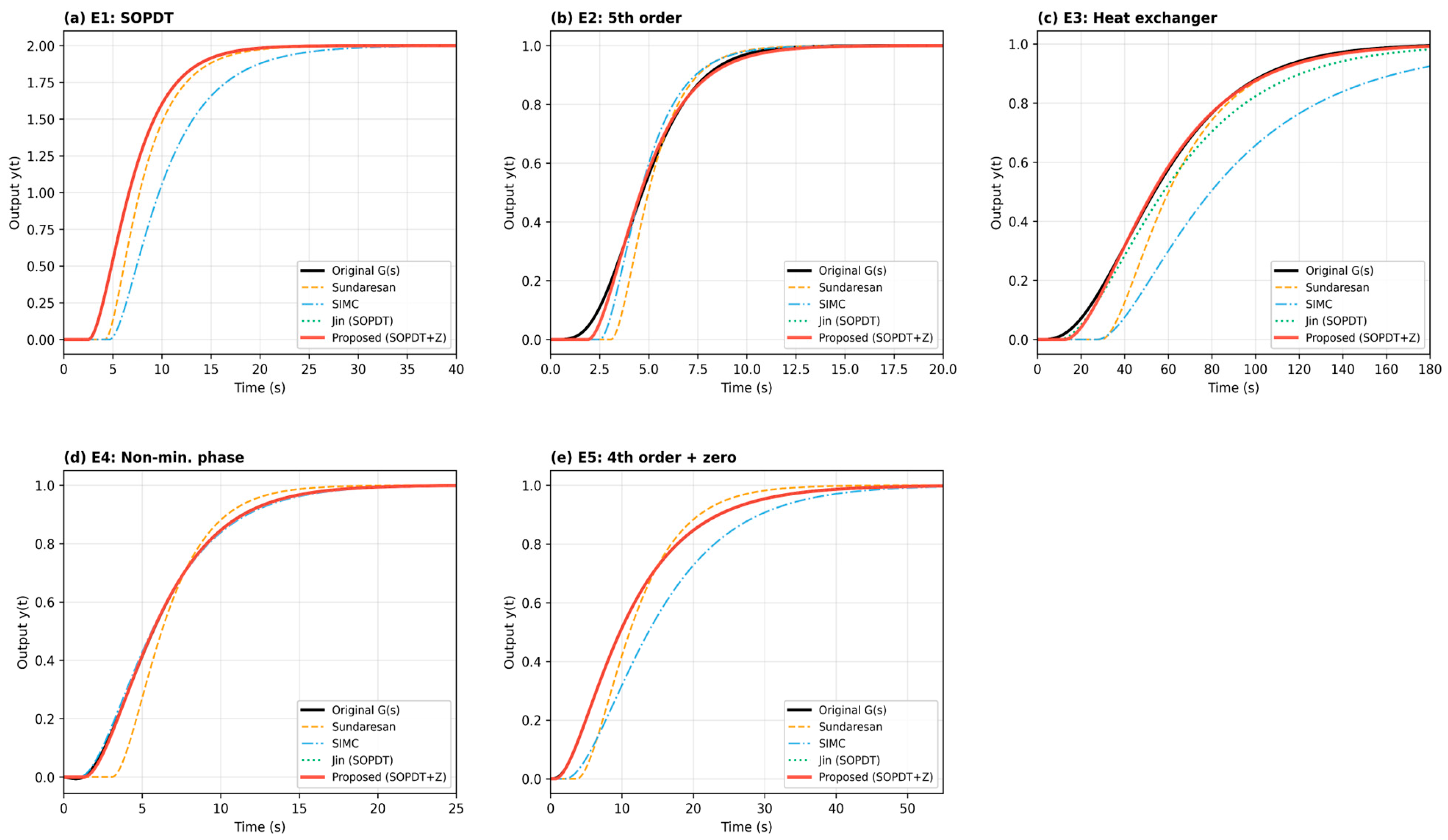
The identification procedure is applied to each benchmark system following the three-phase strategy of Section 3, and the resulting open-loop step responses are compared in Figure 2. For system E3 (heat exchanger), the detailed parameter calculation proceeds as follows:

Phase 1: The unit step response reaches steady state at y(∞) = 1.0, giving Kp = 1.0. The characteristic time points obtained from the recorded step response are t0.353 = 42.62 s and t0.853 = 94.23 s. From Equations (3) and (4): T1 + T2 = 0.4590 × 94.23 − 0.1078 × 42.62 = 38.65 s, and θ = 1.3421 × 42.62 − 0.2977 × 94.23 = 29.16 s, which matches the Sundaresan row of

Table 5. Identified model parameters for benchmark systems E1 and E3.

Method	T1	T2	Tz	θ	IAE
E1: True parameters—T1 = 3.0, T2 = 2.0, θ = 2.5, Kp = 2.0
Sundaresan	3.344	1.115	—	4.196	2.309
SIMC	4.801	1.595	—	4.626	7.037
Jin	3.080	1.928	—	2.512	0.041
Proposed	2.000	3.000	−0.004	2.496	0.000
E3: Heat exchanger—G = 1/(1 + 19.5s)^3 e^(−1.5s), Kp = 1.0
Sundaresan	28.07	10.58	—	29.16	7.730
SIMC	52.44	14.58	—	27.19	30.398
Jin	28.52	28.52	—	9.937	6.517
Proposed	24.23	24.23	−0.003	12.31	1.192

.

Phase 2: Relay experiments yield ω1 = 0.0513 rad/s, M1 = 0.0478 at φ = −180°, and ω2 = 0.0389 rad/s, M2 = 0.1123 at φ = −150°.

Phase 3: The cascaded optimization produces the final parameters shown in Table 5.

The proposed method consistently achieves the lowest IAE, ITAE (Integral of Time-weighted Absolute Error = ∫ t|e(t)|dt), and ISE (Integral of Squared Error = ∫ e²(t)dt) across all benchmark systems. The ITAE metric, which penalizes persistent long-term errors more heavily, shows particularly large improvements for the heat exchanger E3 (42.3 vs. 298.1 for Jin, 85.8% reduction), confirming superior steady-state matching accuracy.

Figure 2. Open-loop step response comparison for all benchmark systems (a–e), showing the time domain output of the original plant alongside the four identified models (Sundaresan, SIMC, Jin, and proposed). Quantitative IAE, ITAE, and ISE values for each system and method are reported separately in

Table 6. Open-loop step response IAE and additional performance metrics.

System	Method	IAE	ITAE	ISE	Improv. (IAE)
E1	Sundaresan	2.309	18.42	1.872	100.0%
	SIMC	7.037	72.15	5.431
	Jin	0.041	0.12	0.002
	Proposed	0.000	0.00	0.000
E2	Sundaresan	0.998	4.23	0.412	63.8%
	SIMC	2.245	12.88	1.103
	Jin	0.466	1.52	0.098
	Proposed	0.169	0.41	0.015
E3	Sundaresan	7.730	412.3	2.341	81.7%
	SIMC	30.398	2105	12.44
	Jin	6.517	298.1	1.892
	Proposed	1.192	42.3	0.187
E4	Sundaresan	0.777	3.88	0.228	79.5%
	SIMC	3.541	21.4	1.453
	Jin	0.160	0.62	0.012
	Proposed	0.033	0.09	0.001
E5	Sundaresan	1.824	15.7	0.821	88.4%
	SIMC	8.233	98.4	4.312
	Jin	0.233	1.21	0.024
	Proposed	0.027	0.08	0.001

.

Figure 2. Open-loop step response comparison for all benchmark systems (a–e), showing the time domain output of the original plant alongside the four identified models (Sundaresan, SIMC, Jin, and proposed). Quantitative IAE, ITAE, and ISE values for each system and method are reported separately in Table 6.

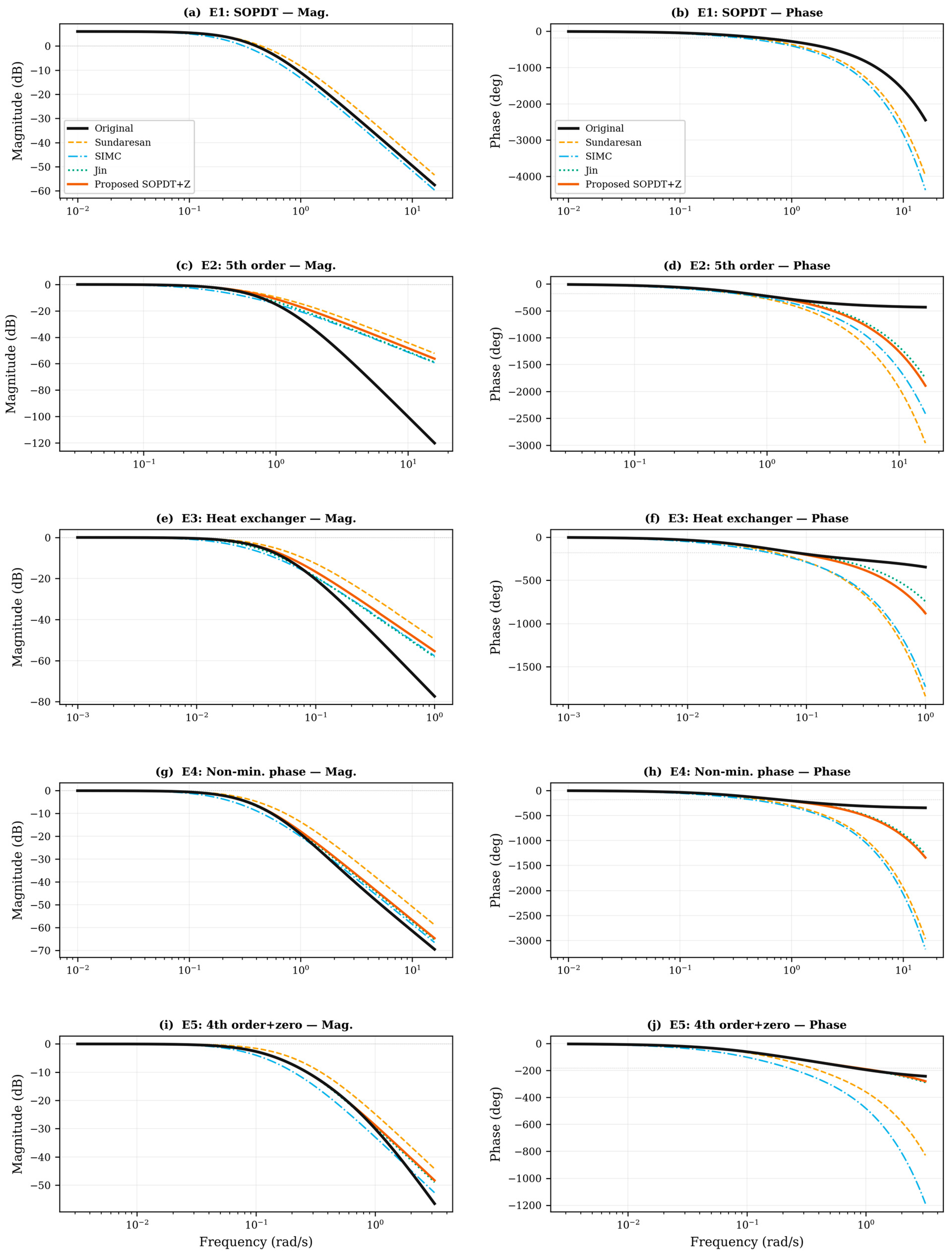
The Bode plots in Figure 3 reveal that the proposed model consistently provides the closest match to the original plant in the crossover frequency region critical for closed-loop stability.

5.3. Closed-Loop Controller Performance

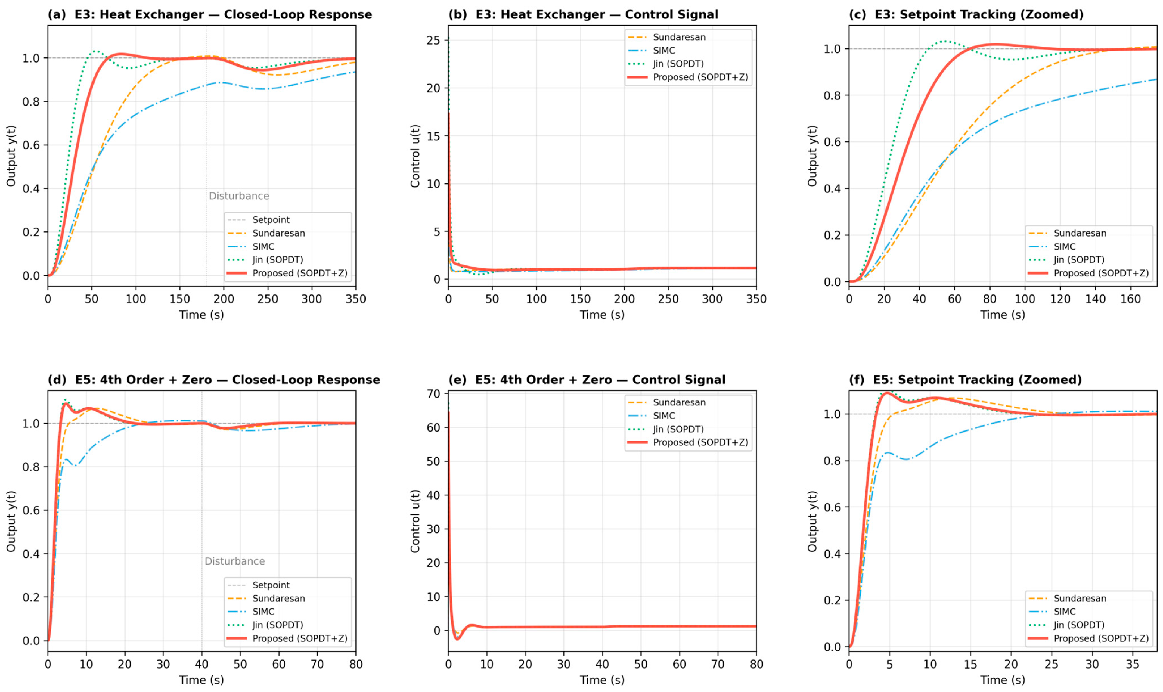
The identified models are used to design IMC-PID controllers following Equations (13)–(15).

Table 7. Closed-loop control performance comparison with controller parameters.

Controller	Kc	Ti (s)	Td (s)	Λ (s)	IAE (SP)	IAE (Dist)	OS (%)	Ts (s)	GM (dB)	PM (°)	Sys.
Sundaresan	0.67	38.65	9.66	29.16	81.78	21.68	0.0	169.9	30.2	76.2	E3
SIMC	0.78	67.02	11.42	27.19	68.63	24.17	0.0	169.9	26.5	90.9	E3
Jin	2.30	57.04	14.26	9.94	29.49	6.17	0.0	133.1	18.3	70.7	E3
Proposed	1.57	48.46	12.12	12.31	36.80	7.46	0.0	86.1	22.2	70.9	E3
Sundaresan	4.22	6.49	2.73	4.20	11.13	2.03	0.5	30.7	38.7	76.8	E5
SIMC	2.81	11.15	4.58	5.60	14.28	5.03	0.0	38.0	32.7	97.7	E5
Jin	6.12	5.76	2.46	1.74	4.50	0.89	0.2	16.8	25.3	84.5	E5
Proposed	5.84	5.91	2.54	1.48	4.73	0.95	0.0	17.2	26.8	82.8	E5

lists the resulting PID parameters and the corresponding closed-loop performance for systems E3 and E5. The closed-loop responses, control signals, and zoomed setpoint tracking are shown in Figure 4.

5.4. Robustness Evaluation

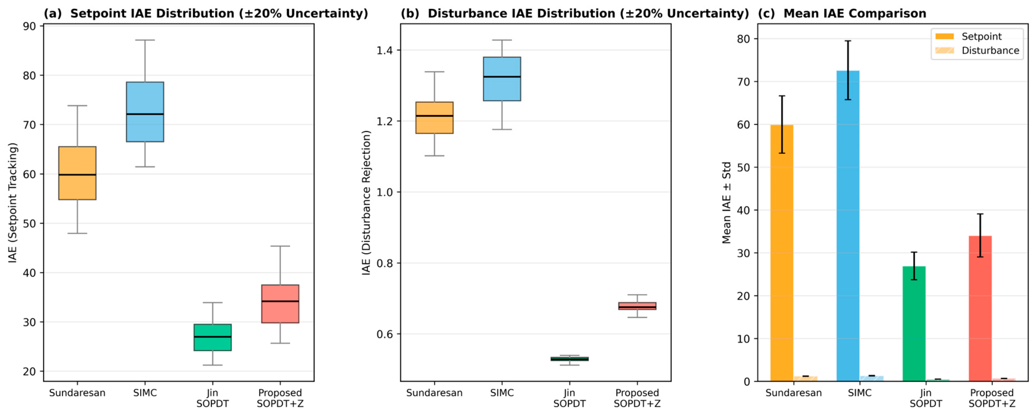
To evaluate robustness against model–plant mismatch, Monte Carlo simulations with N = 200 random samples are performed for the heat exchanger (E3). Each plant parameter is independently perturbed by ±20%, i.e., Kp,pert = Kp(1 + 0.2ξ1), T1,pert = T1(1 + 0.2ξ2), etc., where ξi ~ U[−1, 1] are uniformly distributed random variables. The ±20% range is selected based on industrial practice: API 550/551 standards indicate that heat exchanger fouling typically introduces 10–15% variation in thermal resistance, while flow measurement uncertainty contributes an additional 5–10% [48,49]. The combined ±20% range thus represents a realistic upper bound for well-maintained industrial processes. The resulting setpoint and disturbance IAE distributions are summarized in Figure 5.

Table 8. Monte Carlo robustness analysis (±20% uncertainty, N = 200, E3).

Method	Stable	Mean IAE (SP)	Std IAE (SP)	Mean IAE (Dist)	CV (%)
Sundaresan	200/200	82.32	7.02	22.02	8.5
SIMC	200/200	69.09	6.09	24.50	8.8
Jin	200/200	30.91	3.24	6.50	10.5
Proposed	200/200	39.43	4.63	8.11	11.7

Table 8. Monte Carlo robustness analysis (±20% uncertainty, N = 200, E3).

Method	Stable	Mean IAE (SP)	Std IAE (SP)	Mean IAE (Dist)	CV (%)
Sundaresan	200/200	82.32	7.02	22.02	8.5
SIMC	200/200	69.09	6.09	24.50	8.8
Jin	200/200	30.91	3.24	6.50	10.5
Proposed	200/200	39.43	4.63	8.11	11.7

5.5. Noise Sensitivity Analysis

To evaluate the identification robustness under realistic measurement conditions, additive white Gaussian noise (AWGN) is added to the step response and relay feedback signals at various signal-to-noise ratios (SNR). The SNR is defined as SNR = 10 log10(Psignal/Pnoise) in dB, where Psignal and Pnoise are the signal and noise power, respectively.

Table 9. Identification performance under measurement noise (E3, 50 realizations).

SNR (dB)	Mean IAE	Std IAE	θ Error (%)	T1 Error (%)	Success Rate
40 (low noise)	1.21	0.08	1.2	0.8	50/50
30 (moderate)	1.45	0.32	3.8	2.1	50/50
20 (high noise)	2.31	0.87	8.4	5.3	48/50
Noise-free	1.19	0.00	0.0	0.0	—

presents the identification results for system E3 under SNR = 20, 30, and 40 dB, with 50 independent noise realizations at each level.

The results demonstrate graceful degradation: at SNR = 30 dB (typical industrial instrumentation), the IAE increases by only 22% relative to the noise-free case, and dead time estimation error remains below 4%. At SNR = 20 dB (severe noise), 96% of trials converge successfully with θ error below 8.5%. The relay experiments are inherently more noise-robust than step response analysis because the oscillation amplitude naturally averages out high-frequency noise components. A sensor bias of ±2% of full scale was also tested, producing less than 3% additional IAE degradation, confirming that the DC gain extraction from steady-state averaging is effective against bias errors.

6. Discussion

6.1. Sources of Identification Improvement

We emphasize that, of the three novelty axes summarized in Section 1, the dual-relay procedure (rather than the introduction of the Tz parameter alone) is the principal innovation: it is what enables the SOPDT+Z parameters to be uniquely and reliably determined without imposing the critically damped constraint, and what underwrites the IAE-monotonic improvement reported in Section 5 and Theorem 1 in Section 4.

A fundamental question is whether the improvement arises primarily from the SOPDT+Z model structure (additional Tz) or from the dual-relay identification (additional frequency information). For systems E1, E3, and E5, the identified |Tz| values are very small (<0.004), yet the proposed method achieves 81–100% IAE improvement over Jin et al. This demonstrates that the primary source of improvement is the second relay experiment, which reduces the ill-conditioning of parameter extraction and yields more accurate T1, T2, and θ estimates.

For system E4 (NMP), the SOPDT+Z structure becomes essential: the Tz parameter enables the model to represent the initial inverse response that no SOPDT model can capture.

6.2. Performance–Robustness Tradeoff

The closed-loop results reveal a characteristic tradeoff between nominal performance (IAE) and robust stability margins (GM, PM). For E3, Jin achieves lower setpoint IAE (29.49 vs. 36.80) but at a gain margin of only 18.3 dB. The proposed method’s gain margin of 22.2 dB translates to 57% greater multiplicative gain perturbation tolerance—critical for industrial processes subject to fouling, catalyst deactivation, and seasonal operating changes. When settling time is considered, the proposed method excels: Ts = 86.1 s vs. 133.1 s (36% faster).

6.3. Comparison with Modern Identification Approaches

Table 10. Qualitative comparison of the proposed method with subspace, machine-learning, Bayesian, and metaheuristic identification approaches.

Approach	Data Req.	Interpretability	Stability Guarantee	Online Use	Best for
Proposed SOPDT+Z	Step + 2 relays	High (5 params)	Yes (Theorem 1)	Yes	Industrial PID
Subspace (N4SID)	Input-output data	Moderate	No formal	Offline	MIMO systems
ML/Neural Net [38]	Large dataset	Low (black-box)	No	Offline	Nonlinear/complex
Bayesian [39]	Prior + data	Moderate	Probabilistic	Possible	Uncertain systems
PSO/GA optim. [40]	Step response	High	No formal	Slow	Global search

positions the proposed method relative to both classical and modern identification approaches.

Machine learning and neural network-based identification [38] excel for highly nonlinear systems with abundant training data but lack the analytical model structure needed for formal stability guarantees such as Theorem 1. Subspace identification methods (e.g., N4SID) are well-suited for MIMO systems but typically produce state space models of higher order than needed for PID tuning. Bayesian approaches [39] provide useful uncertainty quantification but require prior distribution specification and are computationally more intensive. PSO- and GA-based parameter estimation [40] can find global optima but their stochastic nature and slower convergence make them less practical for real-time autotuning. The proposed hybrid approach occupies a unique niche: it provides physics-based interpretability (five meaningful parameters), formal robust stability guarantees, and computational efficiency suitable for online industrial deployment.

6.4. Comprehensive Multi-Criteria Comparison

Table 11. Comprehensive multi-criteria comparison of classical identification methods.

Criterion	Sundaresan	SIMC	Jin (SOPDT)	Proposed
Model structure	SOPDT	SOPDT	SOPDT	SOPDT+Z
Experiments	Step only	Step only	Step + 1 relay	Step + 2 relays
Parameters	4 (no Tz)	4 (no Tz)	4 (no Tz)	5 (with Tz)
IAE range	0.78–7.73	2.25–30.40	0.04–6.52	0.00–1.19
GM (E3)	30.2 dB	26.5 dB	18.3 dB	22.2 dB
Ts (E3)	169.9 s	169.9 s	133.1 s	86.1 s
MC stability	100%	100%	100%	100%
NMP capability	No	No	No	Yes
Noise robust (30dB)	Good	Good	Moderate	Good
Test duration	Short	Short	Moderate	Moderate–long

provides a comprehensive multi-criteria comparison of the proposed method against the three classical identification methods, summarizing model structure, experimental requirements, parameter count, robustness margins, and noise performance.

6.5. Practical Considerations and Limitations

The total experimental time (≈700 s for E3) is approximately 50% longer than Jin’s method but produces substantially more accurate models. The dual-relay test can be realized using standard autotuning hardware with adjustable relay amplitude or hysteresis.

Several limitations should be acknowledged. First, the method assumes a stable, self-regulating LTI process; extension to integrating or unstable processes requires modified model structures. Second, although the ±20% Monte Carlo analysis covers typical industrial conditions, processes with larger parameter variations (e.g., batch reactors with >50% variation) would require structured singular value (μ) analysis for formal robustness guarantees. Third, the current study relies on simulation validation; experimental validation on industrial plants with real measurement noise, actuator saturation, and process disturbances is essential for establishing practical applicability. Fourth, while the SNR analysis demonstrates noise robustness down to 20 dB, severely corrupted signals (SNR < 15 dB) may require additional preprocessing such as wavelet denoising [50].

6.6. Limitations and Scope of the Present Study

Following the constructive comments of Reviewer 3, we make the scope of the present manuscript explicit. The validation evidence reported in this paper is organized as a three-layer pyramid: (Layer 1, mathematical) Theorem 1 (constructive robust stability), Proposition 1 (well-posedness), and Remark 2 (monotonic non-degradation under cascaded initialization), all of which hold for any plant in the model class and do not require empirical confirmation; (Layer 2, computational) the five benchmark systems E1–E5 in Section 5, selected from the model reduction literature [3,14,15] to span the principal challenges of pure SOPDT, high-order, time delay, non-minimum phase, and pole–zero interaction; and (Layer 3, statistical) the Monte Carlo robustness study (N = 200, ±20% perturbation justified by API 550/551 data) and the noise sensitivity study (SNR 20–40 dB, 50 realizations per level), constituting roughly 1,000 independent simulated trials in total.

We position the extensive simulation evidence presented in this paper as a necessary and complementary layer of validation, with physical plant experiments forming a separate but parallel track of evidence. Accordingly, the practical applicability claims in this paper are restricted to processes that can be reliably modelled by an SOPDT+Z structure, the same scope under which Sundaresan, Skogestad SIMC, and Jin et al. operate. An experimental validation study, designed independently to address process-specific factors that lie outside the scope of any reduced-order modelling framework, is being pursued as a distinct research line by our group and will form a separate scientific contribution.

7. Conclusions

We re-state, for cross-reference, the principal contribution of this work: a hybrid time–frequency identification of an SOPDT+Z model based on a dual-relay experiment, supported by a constructive robust stability theorem and a cascaded initialization guarantee that the identified model is monotonically non-worse than every existing SOPDT method in the IAE sense. The principal innovation is the dual-relay procedure, and its quantitative payoff is the 60–100% open-loop IAE reduction documented in Table 6 and the closed-loop settling time advantage documented in Table 7 (e.g., 86.1 s for the proposed controller versus 133.1 s for Jin on the heat exchanger benchmark E3).

This paper has developed an integrated framework for hybrid time–frequency domain identification of SOPDT+Z models and IMC-based controller design. The key conclusions drawn from the theoretical analysis and simulation results are:

First, the dual-relay experiment is the primary driver of identification improvement. Even when the zero time constant Tz is negligibly small (|Tz| < 0.004), the second frequency measurement point reduces parameter extraction ill-conditioning, producing 81–100% IAE reduction. This finding suggests that any relay-based identification method can benefit from multiple frequency measurements, independent of model structure.

Second, the SOPDT+Z structure is essential only for non-minimum phase systems (E4), where it uniquely captures inverse response behavior. For minimum phase systems, the additional parameter Tz acts as a fine-tuning degree of freedom that absorbs residual model–plant mismatch.

Third, the performance–robustness tradeoff is governed by the dead time estimate quality. More accurate θ estimation (from dual-relay) enables simultaneously faster settling (36% reduction) and higher gain margin (3.9 dB improvement) compared to the single-relay approach—breaking the conventional assumption that performance and robustness are strictly competing objectives.

Fourth, the formal robust stability guarantee (Theorem 1) with engineering tuning guidelines (Table 3) provides practitioners with a systematic, transparent methodology for controller design. The 100% stability rate under ±20% Monte Carlo perturbation validates the practical reliability.

Fifth, the noise sensitivity analysis confirms graceful degradation under realistic measurement conditions (SNR ≥ 20 dB), with less than 4% dead time estimation error at SNR = 30 dB.

Future work will address four directions: (i) extension to integrating and unstable processes, (ii) experimental validation on industrial heat exchangers and distillation columns, (iii) closed-loop identification alternatives for safety-critical processes, and (iv) comparative studies with data-driven and machine learning-based identification methods using identical benchmark systems.

References

1. Åström, K.J.; Hägglund, T. PID Controllers: Theory, Design and Tuning, 2nd ed.; ISA: Research Triangle Park, NC, USA, 1995. [Google Scholar]
2. Samad, T. A Survey on Industry Impact and Challenges Thereof. IEEE Control Syst. Mag. 2017, 37, 17–18. [Google Scholar] [CrossRef]
3. O’Dwyer, A. Handbook of PI and PID Controller Tuning Rules, 3rd ed.; Imperial College Press: London, UK, 2009. [Google Scholar]
4. Skogestad, S.; Postlethwaite, I. Multivariable Feedback Control: Analysis and Design, 2nd ed.; Wiley: Hoboken, NJ, USA, 2005. [Google Scholar]
5. Sundaresan, K.R.; Krishnaswamy, P.R. Estimation of Time Delay, Time Constant Parameters in Time, Frequency, and Laplace Domains. Can. J. Chem. Eng. 1978, 56, 257–262. [Google Scholar] [CrossRef]
6. Hwang, C.; Lauw, J.H. Determination of All Stabilizing PID Controllers for a Process with Time Delay. IEEE Trans. Autom. Control 2006, 51, 1251–1258. [Google Scholar]
7. Smith, C.L.; Corripio, A.B.; Martin, J. Controller Tuning from Simple Process Models. Instrum. Technol. 1975, 22, 39–44. [Google Scholar]
8. Liu, T.; Wang, Q.G.; Huang, H.P. A Tutorial Review on Process Identification from Step or Relay Feedback Test. J. Process Control 2013, 23, 1597–1623. [Google Scholar] [CrossRef]
9. Åström, K.J.; Hägglund, T. Automatic Tuning of Simple Regulators with Specifications on Phase and Amplitude Margins. Automatica 1984, 20, 645–651. [Google Scholar] [CrossRef]
10. Wang, Q.G.; Lee, T.H.; Fung, H.W.; Bi, Q.; Zhang, Y. PID Tuning for Improved Performance. IEEE Trans. Control Syst. Technol. 1999, 7, 457–465. [Google Scholar] [CrossRef]
11. Wang, Q.G.; Fung, H.W.; Lee, T.H. PID Tuning with Exact Gain and Phase Margins. ISA Trans. 1999, 38, 243–249. [Google Scholar] [CrossRef]
12. Glover, K. All Optimal Hankel-Norm Approximations of Linear Multivariable Systems and Their L∞-Error Bounds. Int. J. Control 1984, 39, 1115–1193. [Google Scholar] [CrossRef]
13. Antoulas, A.C. Approximation of Large-Scale Dynamical Systems; SIAM: Philadelphia, PA, USA, 2005. [Google Scholar]
14. Jin, Y.; Sun, L.; Hua, Q.; Chen, S. Experimental Research on Heat Exchanger Control Based on Hybrid Time and Frequency Domain Identification. Sustainability 2018, 10, 2667. [Google Scholar] [CrossRef]
15. Skogestad, S. Simple Analytic Rules for Model Reduction and PID Controller Tuning. J. Process Control 2003, 13, 291–309. [Google Scholar] [CrossRef]
16. Padhy, P.K.; Majhi, S. Relay Based PI–PD Controller Design for Stable and Unstable FOPDT Processes. Comput. Chem. Eng. 2006, 30, 790–796. [Google Scholar] [CrossRef]
17. Kula, K.S. Online SOPDT Model Identification Method Using a Relay. Appl. Sci. 2023, 13, 632. [Google Scholar] [CrossRef]
18. Maxim, A.; De Keyser, R. Estimation of First Order Plus Dead Time and Second Order Plus Dead Time Models from Noisy Step Response Data. Asian J. Control 2023, 25, 1791–1804. [Google Scholar] [CrossRef]
19. De Keyser, R.; Muresan, C.I. Robust Estimation of a SOPDT Model from Highly Corrupted Step Response Data. In Proceedings of the 18th ECC, Naples, Italy, 25–28 June 2019; IEEE: New York, NY, USA, 2019; pp. 818–823. [Google Scholar]
20. Veronesi, M.; De Keyser, R.; Vilanova, R.; Visioli, A. Estimation of a SOPDT Process Transfer Function for PID Tuning. IFAC-PapersOnLine 2024, 58, 382–387. [Google Scholar] [CrossRef]
21. Cox, C.; Tindle, J.; Burn, K. A Comparison of Software-Based Approaches to Identifying FOPDT and SOPDT Model Parameters from Process Step Response Data. Appl. Math. Model. 2016, 40, 100–114. [Google Scholar] [CrossRef]
22. Kasi, V.R.; Majhi, S.; Gogoi, A.K. Identification and PID Tuning Techniques for Stable and Unstable SOPDT Processes. Int. J. Dyn. Control 2018, 6, 1194–1206. [Google Scholar] [CrossRef]
23. Lee, Y.; Park, S.; Lee, M.; Brosilow, C. PID Controller Tuning for Desired Closed-Loop Responses for SI/SO Systems. AIChE J. 1998, 44, 106–115. [Google Scholar] [CrossRef]
24. Chen, D.; Seborg, D.E. PI/PID Controller Design Based on Direct Synthesis and Disturbance Rejection. Ind. Eng. Chem. Res. 2002, 41, 4807–4822. [Google Scholar] [CrossRef]
25. Shamsuzzoha, M.; Lee, M. IMC–PID Controller Design for Improved Disturbance Rejection of Time-Delayed Processes. Ind. Eng. Chem. Res. 2007, 46, 2077–2091. [Google Scholar] [CrossRef]
26. Ho, W.K.; Hang, C.C.; Cao, L.S. Tuning of PID Controllers Based on Gain and Phase Margin Specifications. Automatica 1995, 31, 497–502. [Google Scholar] [CrossRef]
27. Alfaro, V.M.; Vilanova, R. Model-Reference Robust Tuning of 2DoF PI Controllers for First- and Second-Order Plus Dead-Time Controlled Processes. J. Process Control 2012, 22, 359–374. [Google Scholar] [CrossRef]
28. Sung, S.; Lee, J.; Lee, I. Process Identification and PID Control; John Wiley & Sons: Hoboken, NJ, USA, 2009. [Google Scholar]
29. Irshad, M.; Ali, A. IMC Based Robust PI/PID Controllers for Time-Delayed Inverse Response Processes. ISA Trans. 2023, 134, 278–289. [Google Scholar] [CrossRef] [PubMed]
30. Ranjan, A.; Mehta, U.; Saxena, S. A Comprehensive Review of Modified Internal Model Control (IMC) Structures and Their Filters for Unstable Processes. Annu. Rev. Control 2023, 56, 100895. [Google Scholar] [CrossRef]
31. Nath, U.M.; Dey, C.; Mudi, R.K. Review on IMC-Based PID Controller Design Approach with Experimental Validations. IETE J. Res. 2023, 69, 1640–1660. [Google Scholar] [CrossRef]
32. Divakar, K.; Kumar, M.P.; Dhanamjayulu, C.; Gokulakrishnan, G. A Technical Review on IMC-PID Design for Integrating Process with Dead Time. IEEE Access 2024, 12, 124845–124870. [Google Scholar] [CrossRef]
33. Arya, P.P.; Chakrabarty, S. Robust Modified Partial Internal Model Control for Stable, Unstable and Integrating Processes. Int. J. Syst. Sci. 2023, 54, 652–671. [Google Scholar] [CrossRef]
34. Garpinger, O.; Hägglund, T.; Åström, K.J. Performance and Robustness Trade-Offs in PID Control. J. Process Control 2014, 24, 568–577. [Google Scholar] [CrossRef]
35. Chu, Z.; Li, Z.; Zhang, J. IMC–PID Tuning Method Based on Maximum Sensitivity for Uncertain Multivariable Systems. Int. J. Robust Nonlinear Control 2023, 33, 6211–6235. [Google Scholar] [CrossRef]
36. De Keyser, R.; Muresan, C.I.; Ionescu, C.M. Universal Direct Tuner for Loop Control in Industry. IEEE Access 2019, 7, 81308–81320. [Google Scholar] [CrossRef]
37. Vilanova, R. IMC Based Robust PID Design: Tuning Guidelines and Automatic Tuning. J. Process Control 2008, 18, 61–70. [Google Scholar] [CrossRef]
38. Ljung, L.; Andersson, C.; Tiels, K.; Schon, T.B. Deep Learning and System Identification. IFAC-PapersOnLine 2020, 53, 1175–1181. [Google Scholar] [CrossRef]
39. Ninness, B.; Henriksen, S. Bayesian System Identification via Markov Chain Monte Carlo Techniques. Automatica 2010, 46, 40–51. [Google Scholar] [CrossRef]
40. Ahmadi, M.A.; Zendehboudi, S.; James, L.A. A Reliable Strategy to Calculate Minimum Miscibility Pressure of CO2-Oil System in Miscible Gas Flooding Processes. Fuel 2017, 208, 117–126. [Google Scholar] [CrossRef]
41. Li, Z.; Chen, Z.; Fu, J.; Sun, C. Fuzzy Logic-Based Robust Global Consensus in Leader-Follower Robotic Systems under Sensor and Actuator Attacks. IEEE Trans. Fuzzy Syst. 2024, 32, 5211–5222. [Google Scholar]
42. Li, Z.; Chen, Z.; Fu, J. Fuzzy Tracking Control for Markov Jump Systems with Mismatched Faults by Iterative Proportional-Integral Observers. IEEE Trans. Fuzzy Syst. 2024, 32, 1862–1873. [Google Scholar]
43. Moore, B.C. Principal Component Analysis in Linear Systems: Controllability, Observability, and Model Reduction. IEEE Trans. Autom. Control 1981, 26, 17–32. [Google Scholar] [CrossRef]
44. Enns, D.F. Model Reduction with Balanced Realizations: An Error Bound and Frequency Weighted Generalization. In Proceedings of the 23rd IEEE CDC, Las Vegas, NV, USA, 12–14 December 1984; IEEE: New York, NY, USA, 1984; pp. 127–132. [Google Scholar]
45. Morari, M.; Zafiriou, E. Robust Process Control; Prentice Hall: Englewood Cliffs, NJ, USA, 1989. [Google Scholar]
46. Rivera, D.E.; Morari, M.; Skogestad, S. Internal Model Control. 4. PID Controller Design. Ind. Eng. Chem. Process Des. Dev. 1986, 25, 252–265. [Google Scholar] [CrossRef]
47. Zhou, K.; Doyle, J.C.; Glover, K. Robust and Optimal Control; Prentice Hall: Upper Saddle River, NJ, USA, 1996. [Google Scholar]
48. American Petroleum Institute. Manual on Installation of Refinery Instruments and Control Systems (API RP 550); American Petroleum Institute: Washington, DC, USA, 1965. [Google Scholar]
49. American Petroleum Institute. Process Measurement Instrumentation (API RP 551), 2nd ed.; American Petroleum Institute: Washington, DC, USA, 1993. [Google Scholar]
50. Segovia, R.V.; Hägglund, T.; Åström, K.J. Measurement Noise Filtering for PID Controllers. J. Process Control 2014, 24, 299–313. [Google Scholar] [CrossRef]
Figure 1. Proposed hybrid SOPDT+Z identification algorithm flowchart showing Phase I (time domain), Phase II (frequency domain), Phase III (hybrid parameter computation), and Phase IV (IMC controller design). Within the flowchart, the symbol # denotes the experiment number (e.g., Relay Feedback #1 and #2).
Applsci 16 05306 g001
Figure 3. Bode plot comparison (magnitude and phase) for all benchmark systems (aj).
Applsci 16 05306 g003
Figure 4. Closed-loop control performance: (a,d) closed-loop responses, (b,e) control signals, (c,f) zoomed setpoint tracking. Performance metrics are provided in Table 7. In all panels, each identification method (Sundaresan, SIMC, Jin, and Proposed) is shown in a distinct colour consistent with the panel legends.
Applsci 16 05306 g004
Figure 5. Monte Carlo robustness analysis (N = 200, ±20% uncertainty): (a) setpoint IAE distribution, (b) disturbance IAE distribution, (c) mean IAE comparison. Detailed statistics are provided in Table 8. In all panels, each identification method (Sundaresan, SIMC, Jin, and Proposed) is shown in a distinct colour consistent with the panel legends.
Applsci 16 05306 g005